MERL { A MITSUBISHI ELECTRIC RESEARCH LABORATORY

http://www.merl.com

Markov networks for low-level vision

William T. Freeman and Egon C. Pasztor

MERL, Mitsubishi Electric Research Laboratory

201 Broadway; Cambridge, MA 02139

freeman@merl.com, pasztor@merl.com

TR-99-08 February 1999

Abstract

We seek a learning-based algorithm that applies to various low-level vision

problems. For each problem, we want to �nd the scene interpretation that best

explains image data. For example, we may want to infer the projected velocities

(scene) which best explain two consecutive image frames (image). From syn-

thetic data, we model the relationship between local image and scene regions,

and between a scene region and neighboring scene regions. Three probabilities

are learned, which characterize the low-level vision algorithm: the local prior,

the local likelihood, and the the conditional probabilities of scene neighbors.

Given a new image, we propagate likelihood functions in a Markov network

to infer the underlying scene. We use a factorization approximation, ignor-

ing the e�ect of loops. This yields an e�cient method to infer low-level scene

interpretations, which we always �nd to be stable. We illustrate the method

with di�erent representations, and show it working for three applications: an

explanatory example, motion analysis and estimating high resolution images

from low-resolution ones.

This work may not be copied or reproduced in whole or in part for any commercial purpose. Permission to

copy in whole or in part without payment of fee is granted for nonpro�t educational and research purposes

provided that all such whole or partial copies include the following: a notice that such copying is by per-

mission of Mitsubishi Electric Information Technology Center America; an acknowledgment of the authors

and individual contributions to the work; and all applicable portions of the copyright notice. Copying,

reproduction, or republishing for any other purpose shall require a license with payment of fee to Mitsubishi

Electric Information Technology Center America. All rights reserved.

Copyright c Mitsubishi Electric Information Technology Center America, 1999

201 Broadway, Cambridge, Massachusetts 02139

1. First printing, TR99-08, February, 1999

Markov networks for low-level vision

William T. Freeman and Egon C. PasztorMERL, a Mitsubishi Electric Res. Lab.

201 BroadwayCambridge, MA 02139

freeman, pasztor@merl.com

February 9, 1999

Abstract

We seek a learning-based algorithm that applies to var-ious low-level vision problems. For each problem, wewant to �nd the scene interpretation that best explainsimage data. For example, we may want to infer the pro-jected velocities (scene) which best explain two consec-utive image frames (image). From synthetic data, wemodel the relationship between local image and sceneregions, and between a scene region and neighboringscene regions. Three probabilities are learned, whichcharacterize the low-level vision algorithm: the local

prior, the local likelihood, and the the conditional prob-abilities of scene neighbors. Given a new image, wepropagate likelihood functions in a Markov network toinfer the underlying scene. We use a factorization ap-proximation, ignoring the e�ect of loops. This yieldsan e�cient method to infer low-level scene interpreta-tions, which we always �nd to be stable. We illustratethe method with di�erent representations, and showit working for three applications: an explanatory ex-ample, motion analysis and estimating high resolutionimages from low-resolution ones.

1 Introduction

Our goal is to interpret images, in particular, to solvelow-level vision tasks. Figure 1 shows examples of theproblems we hope to address: interpreting line draw-ings, analyzing motion, and extrapolating resolution.Each task has input image data, which can be a sin-gle image, or a collection of images over time. Fromthat, we want to estimate an underlying scene, whichcould be 3-dimensional shape, optical ow, re ectances,or high resolution detail. We will focus on low-levelscene representations like these that are mapped overspace. Reliable solutions to these vision tasks wouldhave many applications in searching, editing, and in-terpreting images. Machine solutions might give insight

into biological mechanisms.

Much research has addressed these problems, pro-viding important foundations. Because the problemsare under-determined, regularization and statistical es-timation theory are cornerstones (e.g.: [21, 26, 43, 36,39, 27]). Unfortunately, tractable solutions can be dif-�cult to �nd, or are often unreliable or slow. Often-times the statistical models used need to be made-upor hand-tweaked. Various image interpretation prob-lems have de�ed generalization from initial simpli�edsolutions [40, 3, 38].

In part to address the need for stronger models, re-searchers have analyzed the statistical properties of thevisual world. Several groups derived V1-like receptive�elds from ensembles of images [30, 5]; Simoncelli andSchwartz [37] accounted for contrast normalization ef-fects by redundancy reduction. Li and Atick [2] ex-plained retinal color coding by information process-ing arguments. Researchers have developed powerfulmethods to analyze and synthesize realistic textures bystudying the response statistics of V1-like multi-scale,oriented receptive �elds [19, 11, 43, 36]. These meth-ods may help us understand the early stages of imagerepresentation and processing in the brain.

Unfortunately, they don't address how a visual sys-tem might interpret images. To do that, one shouldcollect statistics relating images with their underlyingscene interpretations. This data is di�cult to collectfor natural scenes, since it involves gathering both im-ages and the ground truth data, of the scene attributesto be estimated.

A useful alternative is to use computer graphics togenerate and render synthetic worlds, where every at-tribute is known, and record statistics from those. Sev-eral researchers have done so: Kersten and Knill stud-ied linear shading and other problems [25, 24]; Hurl-bert and Poggio trained a linear color constancy esti-mator [20]. Unfortunately, the simpli�ed (usually lin-ear) models which were used to obtain tractable results

limited the usefulness of these methods.

Our approach is to use general statistical models,but to make the method tractable by restricting our-selves to local regions of images and scenes. We follow alearning-based approach, and use Markov networks toform models of image rendering, and prior probabilitiesfor scenes.

We ask: can a visual system correctly interpret avisual scene if it models (1) the probability that anylocal scene patch generated the local image, and (2)the probability that any local scene is the neighbor toany other? The �rst probabilities allow making sceneestimates from local image data, and the second allowthese local estimates to propagate. This approach leadsto a Bayesian method for low level vision problems,constrained by Markov assumptions. We describe thisgeneral method, illustrate implementation choices, andshow it working for several problems.

Figure 1: Example low-level vision problems. (The

scenes shown are idealizations, not program out-

puts).

2 Bayesian method

We take a Bayesian approach [6, 26]. We want to �ndthe the posterior probability, P (~xj~y): the probability ofa scene, ~x, given the image observation, ~y. By Bayesrule (standard names shown):

P (~xj~y) =P (~yj~x) P (~x)

P (~y)(1)

posterior =likelihood � prior

evidence: (2)

The evidence is independent of the scene, ~x, we wantto estimate, so we treat it as a normalization constant.

The optimum scene estimate, ~̂x, depends on the lossfunction, or the penalty for guessing the wrong scene[6, 12]. Two di�erent choices lead to the estimationrules used here. The Maximum A Posteriori, or MAP,

estimate is the scene, ~̂x, which maximizes the poste-rior, P (~xj~y). The Minimum Mean Squared Error, orMMSE, estimate is the posterior mean. For computa-tional convenience, we will use MMSE with inferencein a continuous representation, and MAP with discreterepresentations.

The likelihood term, P (~yj~x) is the forward model.For a given scene, it asks, what is the probability thatthis scene renders to the observed image data? Theprior probability, P (~x) states how probable a scene isto exist.

The space of all possible solutions is very large. Inprinciple, to �nd the best scene, one needs to ren-der each candidate scene and evaluate its likelihoodand prior probability. To make practical systems, re-searchers typically restrict some aspect of the problem.We will make three major approximations. First, weonly model the statistics of local regions, invoking theMarkov assumption (next section). Second, we will usea factorization approximation (Sect. 3.1) to solve theMarkov model. Finally, our preferred solution is tosample from a continuous distribution (Sect. 4.3) dur-ing the \inference phase".

3 Markov network

We place the image and scene data in a Markov network[31, 17]. We break the images and scenes into localizedpatches where image patches connect with underlyingscene patches; scene patches also connect with neigh-boring scene patches, Fig. 2. (The neighbor relation-ship can be with regard to position, scale, orientation,etc.). This forms a network of scene nodes, each ofwhich may have an associated observation.

Figure 2: Markov network for vision problems.

Observations, y, have underlying scene explana-

tions, x. Connections between nodes of the graphi-

cal model indicate statistical dependencies.

Referring to Fig. 2, the Markov assumption assertsthat complete knowledge of node xj makes nodes xi andxk independent, or P (xi; xkjxj) = P (xijxj)P (xk jxj).We say xi and xk are conditionally independent givenxj . (For notational convenience, we will drop the vec-tor symbol from the random variables.) The Markovassumption also implies that P (xijxj ; xk) = P (xijxj).

This lets us model a complicated spatial probability bya network of (tractable) probabilities governing localrelationships.

To apply a Markov network to vision problems, weneed to �rst learn the parameters of the network from acollection of training examples. Then, given new imagedata, we seek to infer the corresponding scene.

There are exact and approximate methods for boththe learning and inference phases [17, 22, 14]. Exactmethods can be prohibitively time consuming. For net-works without loops, the Markov assumption allows theposterior probability to factorize, yielding e�cient lo-cal rules for both learning and inference [31, 42, 22, 14].We will adopt a factorization approximation, ignoringthe e�ect of loops during both learning and inference.

3.1 Factorization

There are di�erent, equivalent ways to use the Markovassumptions to factorize the posterior probability of aMarkov network without loops [31, 42, 22, 14]. We usea particular factorization, which we believe to be new,which leads to a message passing scheme with appealinginterpretations for the messages [13].

We derive the evidence propagation rules of the in-ference stage by calculating the messages needed toachieve the optimal Bayesian estimate at a scene node.These rules will indicate the probabilities we need tomeasure during the learning phase. We present thederivation for the MMSE estimator, using continuousvariables, then indicate how to modify the rules for theMAP estimator, and for discrete variables.

Before any messages are passed, each node, j, hasonly its local evidence, yj , available for estimatingthe local scene, xj . The best that node can do is tocalculate the mean of the posterior from P (xj jyj) /P (xj ; yj) = P (yj jxj)P (xj). The MMSE estimate atiteration 0, x̂j0, is

x̂j0 =

Zxj

xjP (xj)P (yj jxj): (3)

At the �rst message passing iteration, node j willcommunicate with neighboring scenes. For simplicityof exposition, we assume scene node j has just twoscene neighbors, nodes i and k. Including those obser-vations yi and yk of the neighboring nodes, the MMSEestimate for xj will be the mean over xj of the jointposterior, P (yi; xi; yj ; xj ; yk; xk), after marginalizationover xi and xk :

x̂j1 =

Zxj

xj

Zxi;xk

P (yi; xi; yj ; xj ; yk; xk) (4)

=

Zxj

xj

Zxi;xk

P (yi; xi; yj ; yk; xk jxj)P (xj)(5)

=

Zxj

xjP (xj)P (yj jxj) (6)

�

Zxi

P (yi; xijxj)

Zxk

P (yk; xkjxj): (7)

The factorization of P (yi; xi; yj ; yk; xkjxj) used abovefollows from the conditional independence de�ned bythe Markov network. After marginalizing over xi, themessage

Rxi

P (yi; xijxj) will become P (yijxj), and sim-ilarly for xk. We call this a region likelihood, the like-lihood given xj of some other region of image obser-vations, in this case, just yi. This is a nice feature ofour particular factorization: the messages passed be-tween nodes are all region likelihoods. These are allconditionally independent of each other (given xj), ifthe network has no loops.

To form the full likelihood function for xj , we mul-tiply together all the region likelihoods and the locallikelihood. Multiplying by the local prior, P (xj), thengives the posterior for xj , joint with yj and all the ob-servations that entered into the region likelihoods.

We call P (xj) the local prior, and P (yj jxj) the local

likelihood. P (xijxj) is a scene conditional. Eq. (7) thenhas the form,

x̂j =

Zxj

xj � [local prior] (8)

� [local likelihood] (9)

�Y

neighbor links

[region likelihoods]:(10)

We need to know how to generate new region likeli-hood messages from those received on the previous iter-ation. Let us determine what message node xj shouldpass to node xk. To examine a more general case, as-sume now xj connects to four other scene nodes (seeFig. 7). Suppose node xj receives region likelihoodmessages P (yR1jxj), P (yR2jxj), P (yR3jxj) from eachscene node other than xk . By construction, these re-gions (R1, R2, R3) are conditionally independent ofeach other and of yj , given xj . Thus the region like-lihood for the union of those observations is just theirproduct,

P (yR1; yR2; yR3; yj jxj) = P (yR1jxj)P (yR2jxj)P (yR3jxj)P (yj jxj):(11)

We seek to calculate the next region likelihood mes-sage Lkj = P (yR1; yR2; yR3; yj jxk) to pass to node xk.At each iteration, by adding more image observationsinto the passed region likelihoods, the scene nodes addmore observations to their joint posteriors of observa-tions and scene value, improving their scene estimates.

We will �nd P (yR1; yR2; yR3; yj jxk) by �rst comput-ing P (yR1; yR2; yR3; yj ; xj jxk), then marginalizing overxj . We use P (a; bjc) = P (ajb; c)P (bjc) to write

P (yR1; yR2; yR3; yj ; xj jxk) = (12)

P (yR1; yR2; yR3; yj jxj ; xk)P (xj jxk): (13)

Because xj is closer in the network to the observa-tions in the region likelihood than is xk , by the Markovproperties, we have P (yR1; yR2; yR3; yj jxj ; xk) =P (yR1; yR2; yR3; yj jxj).

Combining our results, we have

P (yR1; yR2; yR3; yj jxk) = (14)Zxj

P (xj jxk)P (yR1jxj)P (yR2jxj)P (yR3jxj)P (yj jxj): (15)

This tells us how to pass region likelihoods from node jto node k: (1) multiply together the region likelihoodsfrom the other neighbors of node j; (2) include nodej's local likelihood; (3) multiply by P (xj jxk); and (4)marginalize over xj . Figure 3 shows the passed mes-sages.

Figure 3: To send a message to node xk, node

xj multiplies together the (conditionally indepen-

dent) region likelihoods for regions R1, R2, and R3,

giving P (yR1; yR2; yR3jxj) (gray arrows show mes-

sages). It multiplies in its own local likelihood,

also conditionally independent of the others, giv-

ing P (yR1; yR2; yR3; yj jxj). After multiplication by

P (xj jxk) and marginalization over xj , that becomes

P (yR4jxk), node xk's region likelihood for the new

region R4 = R1SR2SR3Syj . That is node xj 's

message to node xk, and illustrates one iteration of

recursively passing conditionally independent infor-

mation to neighboring nodes.

Summarizing, after each iteration, the MMSE esti-mate at node j, x̂j is

x̂j =

Zxj

xjP (xj)P (yj jxj)Yk

Lkj ; (16)

where k runs over all scene node neighbors of node j.

We calculate the region likelihoods, Lkj , from:

Lkj =

Zxk

P (xk jxj)P (ykjxk)Yl6=j

~Llk; (17)

where ~Llk is Llk from the previous iteration. The initial~Llk's are 1.

To learn the network parameters, we measure P (xj),P (yj jxj), and P (xkjxj), directly from the synthetictraining data.

3.2 Variations

For a discrete probability representation, we replace theintegral signs with sums. To use the MAP estimator,instead of MMSE, the above arguments hold, with thefollowing two changes:

Zxj

xj ! argmaxxj (18)

Zxi;xk

! maxxi;xk : (19)

3.3 Loops

If the Markov network contains loops, then the re-gion likelihoods arriving at a node are not guaranteedconditionally independent, and the above factorizationmay not hold. Both learning and inference then re-quire more computationally intensive methods. Thereare a range of approximation methods to choose from[22, 14].

One approach is to use non-loopy multi-resolutionquad-tree networks [27], for which the factorizationrules do apply, to propagate information spatially. Un-fortunately, this gives results with artifacts along quad-tree boundaries, statistical boundaries in the model notpresent in the real problem.

We found good results by including the loop-causingconnections between adjacent nodes at the same treelevel but applying the factorized learning and propaga-tion rules, anyway. Others have obtained good resultsusing the same approach for inference [14, 28, 42];

By \unwrapping" the computation of a loopy net-work, Weiss provides theoretical arguments why thisworks for certain networks [42]. Evidence is double-counted, but all evidence ends up being double countedequally. Fig. 4 shows how this multiple counting isdistributed over space, for an array of four-connectednodes. By the (scaled) intensity, the �gure shows thenumber of times each node contributes to the beliefcalculation of the center node.

Clearly, all nodes are not counted equally. One couldavoid this concern by using other approximations forsolving the Markov network, although those would beslower. However, in our experiments, we do not observeproblems frommaking the factorization approximation.We prefer this method because it is fast, and we canidentify clearly what the messages between nodes mean.

It may be the case that for various vision problems,the likelihood functions are essentially binary functions,either zero or not, indicating either a scene interpreta-tion is inconsistent with the observations, or it is con-sistent. For such likelihood functions, the region like-lihoods are always conditionally independent, as is re-quired for the arguments of Sect. 3.1, even for a networkwith loops. (For binary likelihoods, the factorization ofEq. 11 will hold even if observations are counted mul-tiple times.) The behavior of this limiting case mayexplain why we obtain good results using this factor-ization approximation.

(a)

(b)

0

3

6

1

4

7

2

5

8

Figure 4: Plots of the number of times each node

contributes a message to the belief at the center

node, as a function of iteration number. (a) shows

locations contributing to the belief, with arrows in-

dicating which node each message came from. The

nine images of (b) repeat that and continue to itera-

tion 8, plotting one node per square pixel. This view

of the \unwrapped" calculation shows that node

data enters the belief calculation multiple times

(each plot is rescaled).

4 Probability Representations

We have explored di�erent probability representationswith our method, Eqs. (16) and (17): (1) continuous,(2) discrete, and (3) a hybrid method. To explain ourtechnique, in the rest of the paper we present exam-ple applications using each of these three probabilityrepresentations.

4.1 Continuous Representation

We used mixtures of gaussians to represent continuousprobability densities. We �t the densities to trainingdata using EM (Expectation Maximization) [7].

During inference, Eqs. (16) and (17) require mul-tiplying together probability densities. Since gaus-sians multiply together to give gaussians (given by theKalman �ltering formula [16]), the multiplied mixturesyield other mixtures of gaussians.

However, one must merge and prune the gaussians.We tested whether two gaussians of a mixture couldbe merged into one by measuring the Kullback-Leibler(KL) distance [7] between the mixture with the mergedgaussians and the mixture with the non-merged gaus-sians. (We measured the KL distance by sampling, sothere is randomness in our pruning). We repeatedlytesting pairs of gaussians, never repeating comparisonsof a merged mixture with comparisons made by its an-cestors gaussians. This pruning allows iterative cal-culation with continuous densities, using a mixture ofgaussians representation.

4.1.1 Toy Problem

We illustrate this representation, and our technique, fora toy problem with 1-dimensional data. Consider a 3by 3 network of nodes (Fig. 8, (a)) laid out spatially5 units apart. The \scene" we want to estimate is thehorizontal position of each node, which is the same foreach node of a column, and di�erent by 5 units for eachadjacent node in a row. The image data usually tellsthe scene value itself, with a little noise. However, whenthe image data, y = 0, then the underlying scene, x,can take on any value. Figure 5 shows the joint density,P (x; y). This behavior is typical of some vision prob-lems, where local image cues can determine the sceneinterpretation, but other image values give ambiguousinterpretations.

4.1.2 Learning

During learning, we present many examples of imagedata, y, coupled with scene data, x. From those ex-

amples, we used EM to �t mixtures of ten gaussiansto each of the probability densities that de�ne our al-gorithm: the local prior P (xj), the local likelihood,P (yj jxj), and the scene conditionals, P (xleftjx), andP (xabovejx). Figure 6 shows the �tted mixtures.

Figure 5: Illustrative toy problem, joint probability

densities. x is the scene data; y is the corresponding

observation. y is a good indicator of the underlying

scene, except when y = 0; then the scene can be

anything.

(a)

(b)

(c)

(d)

Figure 6: Outputs of learning phase for toy prob-

lem of Sect. 4.1.1. All probability densities shown

are mixtures of gaussians, �tted to labelled train-

ing data. Both scene, x, and image, y, variables

are 1-d here. (a) Local prior (red shows component

gaussians of mixture, blue is sum). Fit is only ap-

proximate to the true prior (vertical projection of

Fig. 5), but adequate for inference. (b), (c) and

(d): Learned conditionals for P (yjx), P (xleftjx),

P (xabovejx). Jumps to horizontally neighboring

node changes x by 5 units. Jumps to vertical neigh-

bors leave x constant. The learned conditionals (c)

and (d) both correctly model this made-up world.

4.1.3 Inference

Given particular image data (Fig. 8 (a)), we infer theunderlying scene values for our toy problem by itera-tively applying Eqs. (16) and (17). Figures 7 and 8illustrate the message passing and belief calculation.Figures 9 { 12 show the posterior probabilities at eachnode for 0, 1, 2, and 10 iterations. By iteration 2, eachnode has communicated with node 5 (which has un-ambiguous local image information). Each node thenhas the correct posterior mean. After 10 iterations,the spreads of the posterior probability peaks are arti�-cially narrowed, from treating as conditionally indepen-dent messages passed around through loops. However,the posterior means maintain their proper values.

4.2 Discrete representation

The continuous representation used above is appealing,but inference is very slow for larger problems. Fur-thermore, the necessary repeated pruning of gaussianmixtures reduces the modeling accuracy.

To correct those problems, one might consider usinga discrete representation. Then the basic calculationsin the inference equations, Eqs. (16) and (17), become(fast) vector and matrix multiplications. In this sec-tion, we show the result of a discrete representation,illustrating another application domain: motion analy-sis. Here the \image" is two concatenated image framesat sequential times. The \scene" is the correspondingprojected velocites in each frame.

The training images were randomly generated mov-ing, irregularly shaped blobs, as typi�ed by Fig. 13 (a).The contrast with the background was randomized.Each blob was moving in a randomized direction, atsome speed between 0 and 2 pixels per frame.

We represented both the images and the velocities in4-level Gaussian pyramids [9], to e�ciently communi-cate across space. Each scene patch then additionallyconnects with the patches at neighboring resolution lev-els. Figure 13 shows the multiresolution representation(at one time frame) for images and scenes.1

We applied the training method and propagationrules to motion estimation, using a vector code rep-resentation [18] for both images and scenes. We wrotea tree-structured vector quantizer, to code 4 by 4 pixelby 2 frame blocks of image data for each pyramid levelinto one of 300 codes for each level. We also codedscene patches into one of 300 codes. Figure 13 showsan input test image, (a) before and (b) after vector

1To maintain the desired conditional independence relation-

ships, we appended the image data to the scenes. This provided

the scene elements with image contrast information, which they

would otherwise lack.

quantization. The true underlying scene, the desiredoutput, is shown at the right, (a) before and (b) aftervector quantization.

4.2.1 Learning

During learning, we presented approximately 200,000examples of di�erent moving blobs, some overlapping,of a contrast with the background randomized to one of4 values. Using co-occurance histograms, we measuredthe statistical relationships that embody our algorithm:P (x), P (yjx), and P (xnjx), for scene xn neighboringscene x. Figures. 14 and 15 show examples of thesemeasurements.

4.2.2 Inference

Figure 16 shows six iterations of the inference algorithm(Eqs. 16 and 17) as it converges to a good estimate forthe underlying scene velocities. The local probabilitieswe learned (P (x), P (yjx), and P (xnjx)) lead to �g-ure/ground segmentation, aperture problem constraintpropagation, and �lling-in (see caption). The resultinginferred velocities are correct within the accuracy of thevector quantized representation.

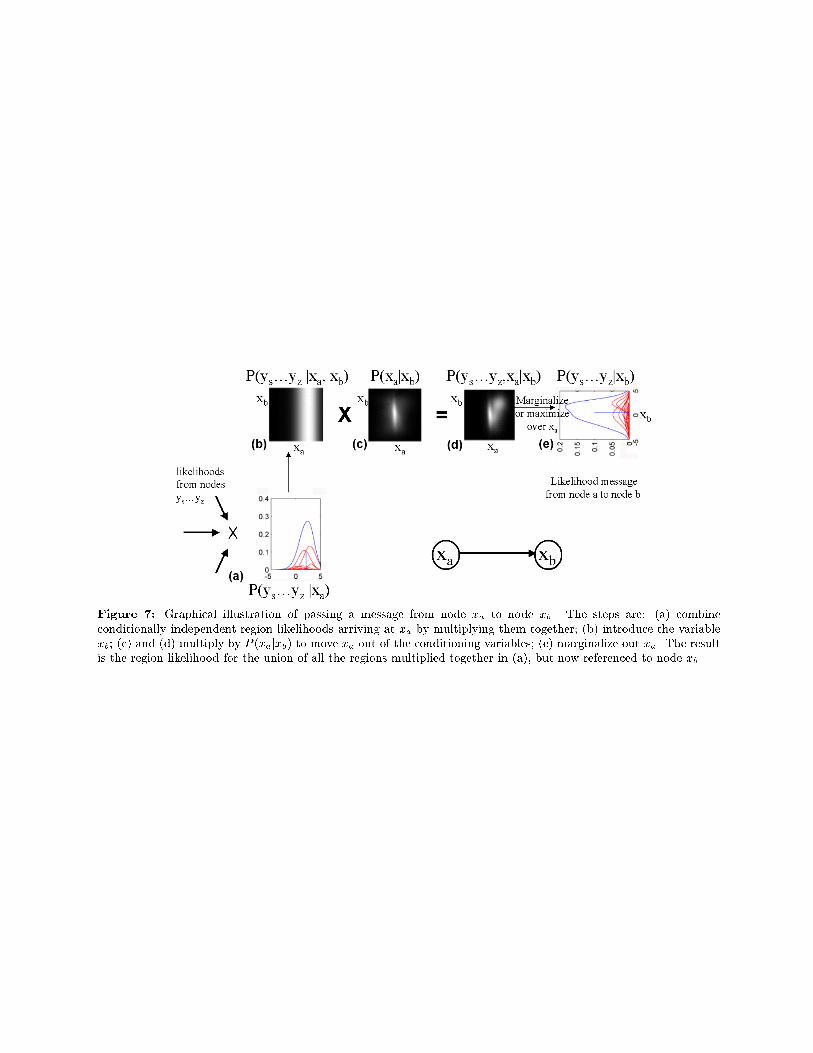
Figure 7: Graphical illustration of passing a message from node xa to node xb. The steps are: (a) combine

conditionally independent region likelihoods arriving at xa by multiplying them together; (b) introduce the variable

xb; (c) and (d) multiply by P (xajxb) to move xa out of the conditioning variables; (e) marginalize out xa. The result

is the region likelihood for the union of all the regions multiplied together in (a), but now referenced to node xb.

(a)

(b)

Figure 8: (a) Observed data for scene inference, for toy problem. (b) Belief calculation at a node (node 5), �rst

iteration. The belief is the product of six probability distributions over x5: the prior on x (P (x5)), the local likelihood

(P (y5 = 3jx5)), and the four region likelihoods, which are messages passed from nodes 2, 4, 6, and 8.

Figure 9: Next four �gures: posterior distributions at each node of toy problem of Sect. 4.1.1, over several iterations.

Figure 8 (a) shows the \image" data. Iteration 0: initial beliefs at each node before any message passing. The

observations at all nodes have ambiguous interpretations, except for node 5, where y = 3 ) x = 3, by the joint

density of Fig. 5. Sampling is used when pruning the gaussian mixtures, so each pruned mixture (of the nodes other

than 5) looks di�erent.

Figure 10: Beliefs at iteration 1. Nodes 2, 4, 6, and 8 have bene�tted from the message passed from node 5.

Figure 11: Beliefs at iteration 2. All nodes have heard the message from node 5. The posteriors have all attained

their proper mean values (-2 for left column of nodes, 3 for middle column, 8 for right column).

Figure 12: Beliefs at iteration 10. Running for 10 iterations arti�cially narrows the posterior distributions, from

hearing the same information many times as if new, due to the network loops. However, the mean values are still the

correct ones.

(a)

(b)Figure 13: Motion estimation problem. (a) First of two frames of image data (in gaussian pyramid), and corre-

sponding frames of velocity data. (b) Image and scene representations after vector quantization. The left side shows

just one of two image frames. The right side shows (red) motion vectors from the second time frame obscuring (blue)

motion vectors from the �rst. The scene representation contains both frames. Each large grid square is one node of

the Markov network.

Figure 14: The local likelihood information for motion problem, vector quantized representation. Conditional

probabilities are derived from co-occurance histograms. For a given image data sample, (a), the 4 most likely scene

elements are shown in (b).

Figure 15: Some scene conditional probabilities, for the motion problem. For the given scene element, (a), the 4

most likely nodes from four di�erent neighboring scene elements are shown. Scene elements also connect to each

other across scale, not shown in this �gure.

Figure 16: The most probable scene code for Fig. 13b at �rst 6 iterations of Bayesian belief propagation. (a)

Note initial motion estimates occur only at edges. Due to the \aperture problem", initial estimates do not agree.

(b) Filling-in of motion estimate occurs. Cues for �gure/ground determination may include edge curvature, and

information from lower resolution levels. Both are included implicitly in the learned probabilities. (c) Figure/ground

still undetermined in this region of low edge curvature. (d) Velocities have �lled-in, but do not yet all agree. (e)

Velocities have �lled-in, and agree with each other and with the correct velocity direction, shown in Fig. 13.

4.3 Continuous learning, sampled infer-

ence

Figure 17: \Lineup of suspects" method for infer-

ence. (Photo from [1]). At each node, we gather a

set of scenes, each of which explains the observed

local image data. We evaluate the scene posterior

only at those sample scenes. We sample appropri-

ately from the continuous representation of the con-

ditional probability with neighboring scenes to ob-

tain discrete linking matrices between nodes. This

allows for fast inference calculations in Eqs. 16 and

17.

Unfortunately, in a discrete representation, a faith-ful image representation requires so many vector codesthat it becomes infeasible to measure the prior and co-occurance statistics. Note unfaithful �t of the vectorquantized image and scene in Fig. 13. On the otherhand, the discrete representation allows fast propaga-tion during inference. We developed a hybrid methodthat allows both good �tting and fast propagation.We use a continuous representation during the learning

phase, and a sampled one during inference.

We illustrate this favored method with a third ap-plication, \super-resolution". For super-resolution,the input \image" is the high-frequency components(sharpest details) of a sub-sampled image. The \scene"to be estimated is the high-frequency components of thefull-resolution image, Fig. 19.

We describe the image and scene patches as vectorsin a continuous space, and model the probability densi-ties, P (x), P (y; x), and P (xn; x), as gaussian mixtures[7]. (We reduced the dimensionality of the scene andimage data within each patch by principal componentsanalysis [7]). We had approximately 20,000 patch sam-ples from our training data, and typically used 9 di-mensional representations for both images and scenes.

During inference, we evaluated the prior and condi-tional distributions of Eq. 17 only at a discrete set ofscene values, di�erent for each node. (This approachwas inspired by the success of other sample-based meth-ods [21, 11]). The scenes were a sampling of thosescenes which render to the image at that node. Wethink of it as a \lineup of suspects", Fig. 17. Each nodehas its own set of suspects. Each scene in a node'slineup has in common the fact that it renders to theimage observation at that node. We evaluate the likeli-hoods of the inference equations, Eqs. 16 and 17, onlyat those scene values for each node. This focusses ourcomputation to just the locally feasible scene interpre-tations.

P (xkjxj) in Eq. 17 becomes the ratios of the gaus-sian mixtures P (xk; xj) and P (xj), evaluated at thescene samples at nodes k and j, respectively. P (ykjxk)is P (yk; xk)=P (xk) evaluated at the scene samples ofnode k. This shows the bene�t of our hybrid approach.To �t the image and scene well, each sample (suspect)has to have a very small bin of continuous parametervalues that map to it. It would be prohibitive to learnthe occurance and cooccurance statistics of such a �ne-grain set of samples; one would have to wait foreverfor scene values to fall in those bins. So we do ourlearning in the continuous domain, where we can inter-polate across parameter values, and do our inferencein a discrete domain, where the calculations reduce tomatrix operations. This \continuous learning/sampledinference" approach reduced the processing times from24 hours to 10 or 15 minutes for the super-resolutionproblem.

To select the scene samples, we could condition themixture P (y; x) on the y observed at each node, andsample x's from the resulting mixture of gaussians.We obtained somewhat better results by using thescenes from the training set whose images most closelymatched the image observed at that node. This avoidedone gaussian mixture modeling step; our sampled infer-

ence actually gave better results than inference in thecontinuous representation.

Using 20 scene samples per node, setting up theP (xk jxj) linking matrix for each link took about 10minutes for these images (approximately 1000 nodes).The scene (high resolution) patch size was 3x3; the im-age (low resolution) patch size was 7x7. We didn't feellong-range scene propagation was critical here, so weused a at, not a pyramid, node structure. Once thelinking matrices were computed, the iterations of Eq. 17were completed in a few minutes.

We performed experiments on two di�erent sourcesof images, synthetic and natural. For a controlled train-ing set, we trained on images of synthetically gener-ated shaded and painted blobs, typi�ed by Fig. 19 (a).Our training data were pairs of band-pass and high-frequency samples such as those shown in Fig. 18. Weused local contrast normalization to reduce the vari-ations we needed to model. Figure 19 illustrates theimage processing steps and the reconstructed result.

Figure 20 shows the bandpassed results after 0, 1, 2,and 20 iterations of the algorithm. (This is the detailwe add to Fig. 19 (c) to get Fig. 19 (d). After few iter-ations, the MAP estimate of the high resolution imageis visually close to the actual full frequency image. Thedominant structures are all in approximately the cor-rect position. This may enable high quality zoomingof low-resolution images, attempted with limited suc-cess by others [35, 32]. To illustrate that the problemis non-trivial, we include the nearest neighbor solutionin Fig. 20. The choppiness there (and at iteration 0,before message passing) shows there are many di�er-ent high-resolution scenes corresponding to any givenlow-resolution image patch.

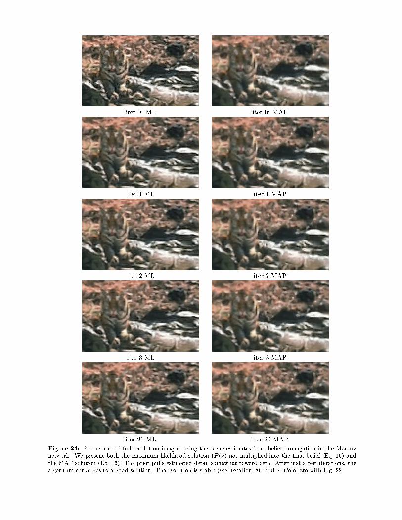
In our second super-resolution experiment, wetrained with images of tigers in the wild, from the Coreldatabase. (Given the success of multi-resolution tex-ture synthesis algorithms [19, 11, 43, 36], we wonderedif high resolution texture scene components might belearned and synthesized). Figure 22 shows the fre-quency components of the image, and Figs. 24 and 25show results. (Figure 23 is the result of a simple com-parison algorithm, the nearest neighbor. The choppi-ness points out that given image data can have multiplepossible local scene interpretations, requiring spatialpropagation of some sort.) Good edge and texture syn-thesis in parts of Fig. 24 provide encouragement thatthis approach might be useful even for textured images.The solution is stable, and reaches convergence quickly.

For comparison, we show the processing result ob-tained using 5 samples (suspects) per node, instead of20, Fig. 25. As might be expected, the result is a bitchoppier.

To test the generalization ability, we used the prob-abilities trained on the tiger images with a non-tigerimage, that of the teapot of Fig. 26. The tiger databasecontained few sharp, crisp edges, and the edges are notextrapolated well in the result. However, the results aregood enough to show that the learned relationships be-tween scenes and images generalizes some beyond strictimage classes.

5 Discussion

In related applications of Markov random �elds to vi-sion, researchers often use relatively simple, heuristi-cally derived expressions (rather than learned) for thelikelihood function P (yjx) or for the spatial relation-ships in the prior term on scenes [17, 33, 15, 24, 8, 27,26, 34]. For other learning or constraint propagationapproaches in motion analysis, see [27, 29, 23].

Weiss showed the advantage of belief propagationover regularization methods for several 1-d problems[41]; we are applying related methods to our 2-d prob-lems.

The local probabilities we measure (local prior andlikelihood, and conditional probability of neighboringscenes) have power and exibility. For the motion prob-lem, they lead to �lling-in motion estimates in a di-rection perpendicular to object contours, Fig. 16 (a){(c). For the super-resolution problem, those same cor-responding probabilities lead to contour completion inthe direction of the contours, Fig. 20 (d){(f). The samelearning machinery was used in each case, but trainedfor di�erent problems, achieving di�erent behavior, ap-propriate to each problem.

An appealing feature of this work is that it instanti-ates many of the intuitions developed vision researcherssome time ago. We spatially propagate local interpre-tation hypotheses in the spirit of blocks world [40, 10]scene interpretation and the work of Barrow and Tenen-baum on intrinsic images [3, 4].

6 Summary

We have presented a general, learning-based methodto solve low-level vision problems. The essence of thealgorithm is measuring three probabilities in a synthet-ically generated labelled world: the local prior, the lo-cal likelihood, and the conditional relationship betweenscene neighbors. We placed image and scene regions ina Markov network. We used a factorization approxima-tion to solve the network: we propagated informationas if the network had no loops. This propagation isfast, and the messages passed between nodes are in-

9639

11104

11155

5494

114

4321

4848

5889

364

6570

4769

799

5619

610

3685

8921

10474

5322

7035

883

9546

6014

416

11663

10026

5032

10809

7536

735

11101

4372

12037

9134

334

11057

3787

9718

1367

10177

9382

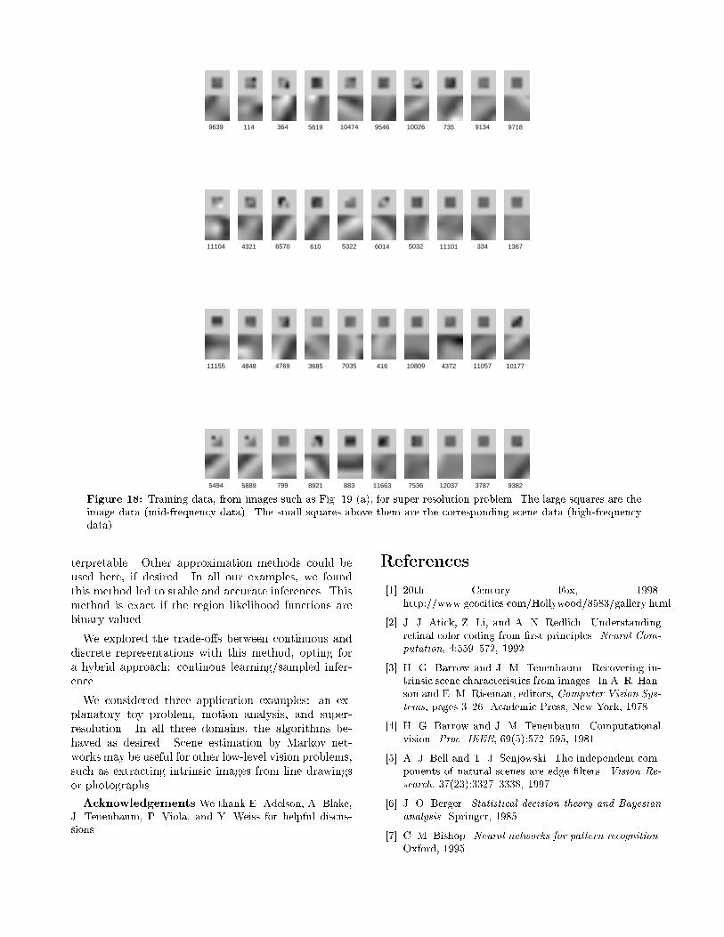
Figure 18: Training data, from images such as Fig. 19 (a), for super-resolution problem. The large squares are the

image data (mid-frequency data). The small squares above them are the corresponding scene data (high-frequency

data).

terpretable. Other approximation methods could beused here, if desired. In all our examples, we foundthis method led to stable and accurate inferences. Thismethod is exact if the region likelihood functions arebinary valued.

We explored the trade-o�s between continuous anddiscrete representations with this method, opting fora hybrid approach: continous learning/sampled infer-ence.

We considered three application examples: an ex-planatory toy problem, motion analysis, and super-resolution. In all three domains, the algorithms be-haved as desired. Scene estimation by Markov net-works may be useful for other low-level vision problems,such as extracting intrinsic images from line drawingsor photographs.

Acknowledgements We thank E. Adelson, A. Blake,

J. Tenenbaum, P. Viola, and Y. Weiss for helpful discus-

sions.

References

[1] 20th Century Fox, 1998.

http://www.geocities.com/Hollywood/8583/gallery.html.

[2] J. J. Atick, Z. Li, and A. N. Redlich. Understanding

retinal color coding from �rst principles. Neural Com-

putation, 4:559{572, 1992.

[3] H. G. Barrow and J. M. Tenenbaum. Recovering in-

trinsic scene characteristics from images. In A. R. Han-

son and E. M. Riseman, editors, Computer Vision Sys-

tems, pages 3{26. Academic Press, New York, 1978.

[4] H. G. Barrow and J. M. Tenenbaum. Computational

vision. Proc. IEEE, 69(5):572{595, 1981.

[5] A. J. Bell and T. J. Senjowski. The independent com-

ponents of natural scenes are edge �lters. Vision Re-

search, 37(23):3327{3338, 1997.

[6] J. O. Berger. Statistical decision theory and Bayesian

analysis. Springer, 1985.

[7] C. M. Bishop. Neural networks for pattern recognition.

Oxford, 1995.

(a) Full resolution (b) Sub-sampled

(c) After blurring (d) Estimated full res.

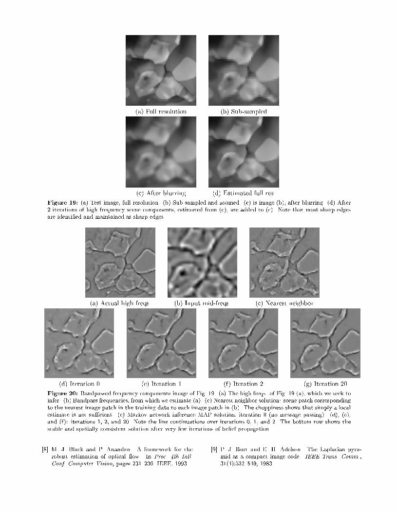
Figure 19: (a) Test image, full resolution. (b) Sub-sampled and zoomed. (c) is image (b), after blurring. (d) After

2 iterations of high frequency scene components, estimated from (c), are added to (c). Note that most sharp edges

are identi�ed and maintained as sharp edges.

(a) Actual high freqs. (b) Input mid-freqs. (c) Nearest neighbor

(d) Iteration 0 (e) Iteration 1 (f) Iteration 2 (g) Iteration 20

Figure 20: Bandpassed frequency components image of Fig. 19. (a) The high freqs. of Fig. 19 (a), which we seek to

infer. (b) Bandpass frequencies, from which we estimate (a). (c) Nearest neighbor solution: scene patch corresponding

to the nearest image patch in the training data to each image patch in (b). The choppiness shows that simply a local

estimate is not su�cient. (c) Markov network inference MAP solution, iteration 0 (no message passing). (d), (e),

and (f): iterations 1, 2, and 20. Note the line continuations over iterations 0, 1, and 2. The bottom row shows the

stable and spatially consistent solution after very few iterations of belief propagation.

[8] M. J. Black and P. Anandan. A framework for the

robust estimation of optical ow. In Proc. 4th Intl.

Conf. Computer Vision, pages 231{236. IEEE, 1993.

[9] P. J. Burt and E. H. Adelson. The Laplacian pyra-

mid as a compact image code. IEEE Trans. Comm.,

31(4):532{540, 1983.

Figure 21: Three random draws from the Corel database set of \tigers" images, used as the training set for Figs. 24,

25, and 26. The training database consisted of 80 images like these. (The test image of Fig. 24 was excluded).

(a) input (b) desired output

(c) image (d) scene

Figure 22: We want to estimate (b) from (a). The original image, (b) is blurred, subsampled, then interpolated

back up to the original resolution to form (a). The missing high frequency detail, (b) - (a), is the \scene" to be

estimated, (d) (this is the �rst level of a Laplacian pyramid [9]). The low frequencies of (a) are removed to form

the input \image", (c). To reduce the variability that the model needs to learn, we form a local contrast image

from the \image" band and use that to scale the image and scene bands before modeling. That scaling is undone at

reconstruction.

[10] M. B. Clowes. On seeing things. Arti�cial Intelligence,

2:79{116, 1971.

[11] J. S. DeBonet and P. Viola. Texture recognition us-

ing a non-parametric multi-scale statistical model. In

Proc. IEEE Computer Vision and Pattern Recognition,

1998.

[12] W. T. Freeman and D. H. Brainard. Bayesian decision

theory, the maximum local mass estimate, and color

constancy. In Proc. 5th Intl. Conf. on Computer Vi-

sion, pages 210{217. IEEE, 1995.

[13] W. T. Freeman and E. C. Pasztor. Learning to es-

timate scenes from images. In M. S. Kearns, S. A.

Solla, and D. A. Cohn, editors, Adv. Neural Informa-

tion Processing Systems, volume 11, Cambridge, MA,

1999. MIT Press.

[14] B. J. Frey. Bayesian networks for pattern classi�ca-

tion. MIT Press, 1997.

[15] D. Geiger and F. Girosi. Parallel and deterministic

algorithms from MRF's: surface reconstruction. IEEE

Pattern Analysis and Machine Intelligence, 13(5):401{

412, May 1991.

[16] A. Gelb, editor. Applied optimal estimation. MIT

Press, 1974.

[17] S. Geman and D. Geman. Stochastic relaxation,

Gibbs distribution, and the Bayesian restoration of

images. IEEE Pattern Analysis and Machine Intel-

ligence, 6:721{741, 1984.

[18] R. M. Gray, P. C. Cosman, and K. L. Oehler. Incor-

porating visual factors into vector quantizers for image

compression. In A. B. Watson, editor, Digital images

and human vision. MIT Press, 1993.

[19] D. J. Heeger and J. R. Bergen. Pyramid-based texture

analysis/synthesis. In ACM SIGGRAPH, pages 229{

236, 1995. In Computer Graphics Proceedings, Annual

Conference Series.

[20] A. C. Hurlbert and T. A. Poggio. Synthesizing a color

algorithm from examples. Science, 239:482{485, 1988.

nearest neighbor solution

Figure 23: Nearest neighbor solution, using the high frequency components of the nearest neighbor in the training

data to each image patch. The result is too choppy, showing that a solution based on local information alone is not

su�cient.

[21] M. Isard and A. Blake. Contour tracking by stochastic

propagation of conditional density. In Proc. European

Conf. on Computer Vision, pages 343{356, 1996.

[22] M. I. Jordan, editor. Learning in graphical models.

MIT Press, 1998.

[23] S. Ju, M. J. Black, and A. D. Jepson. Skin and bones:

Multi-layer, locally a�ne, optical ow and regulariza-

tion with transparency. In Proc. IEEE Computer Vi-

sion and Pattern Recognition, pages 307{314, 1996.

[24] D. Kersten. Transparancy and the cooperative com-

putation of scene attributes. In M. S. Landy and

J. A. Movshon, editors, Computational Models of Vi-

sual Processing, chapter 15. MIT Press, Cambridge,

MA, 1991.

[25] D. Kersten, A. J. O'Toole, M. E. Sereno, D. C. Knill,

and J. A. Anderson. Associative learning of scene pa-

rameters from images. Applied Optics, 26(23):4999{

5006, 1987.

[26] D. Knill and W. Richards, editors. Perception as

Bayesian inference. Cambridge Univ. Press, 1996.

[27] M. R. Luettgen, W. C. Karl, and A. S. Willsky. E�-

cient multiscale regularization with applications to the

computation of optical ow. IEEE Trans. Image Pro-

cessing, 3(1):41{64, 1994.

[28] D. J. C. Mackay and R. M. Neal. Good error{

correcting codes based on very sparse matrices. In

Cryptography and coding { LNCS 1025, 1995.

[29] S. Nowlan and T. J. Senjowski. A selection model for

motion processing in area MT of primates. J. Neuro-

science, 15:1195{1214, 1995.

[30] B. A. Olshausen and D. J. Field. Emergence of simple-

cell receptive �eld properties by learning a sparse code

for natural images. Nature, 381:607{609, 1996.

[31] J. Pearl. Probabilistic reasoning in intelligent systems:

networks of plausible inference. Morgan Kaufmann,

1988.

[32] A. Pentland and B. Horowitz. A practical approach

to fractal-based image compression. In A. B. Watson,

editor, Digital images and human vision. MIT Press,

1993.

[33] T. Poggio, V. Torre, and C. Koch. Computational vi-

sion and regularization theory. Nature, 317(26):314{

139, 1985.

[34] E. Saund. Perceptual organization of occluding con-

tours of opaque surfaces. In CVPR '98 Workshop on

Perceptual Organization, Santa Barbara, CA, 1998.

[35] R. R. Schultz and R. L. Stevenson. A Bayesian ap-

proach to image expansion for improved de�nition.

IEEE Trans. Image Processing, 3(3):233{242, 1994.

[36] E. P. Simoncelli. Statistical models for images: Com-

pression, restoration and synthesis. In 31st Asilomar

Conf. on Sig., Sys. and Computers, Paci�c Grove, CA,

1997.

[37] E. P. Simoncelli and O. Schwartz. Modeling surround

suppression in V1 neurons with a statistically-derived

normalization model. In Adv. in Neural Information

Processing Systems, volume 11, 1999.

[38] P. Sinha and E. H. Adelson. Recovering re ectance

and illumination in a world of painted polyhedra. In

Proc. 4th Intl. Conf. Comp. Vis., pages 156{163. IEEE,

1993.

[39] R. Szeliski. Bayesian Modeling of Uncertainty in Low-

level Vision. Kluwer Academic Publishers, Boston,

1989.

[40] D. Waltz. Generating semantic descriptions from

drawings of scenes with shadows. In P. Winston, ed-

itor, The psychology of computer vision, pages 19{92.

McGraw-Hill, New York, 1975.

[41] Y. Weiss. Interpreting images by propagating Bayesian

beliefs. In Adv. in Neural Information Processing Sys-

tems, volume 9, pages 908{915, 1997.

[42] Y. Weiss. Belief propagation and revision in networks

with loops. Technical Report 1616, AI Lab Memo,

MIT, Cambridge, MA 02139, 1998.

[43] S. C. Zhu and D. Mumford. Prior learning and Gibbs

reaction-di�usion. IEEE Pattern Analysis and Ma-

chine Intelligence, 19(11), 1997.

iter 0: ML iter 0: MAP

iter 1 ML iter 1 MAP

iter 2 ML iter 2 MAP

iter 3 ML iter 3 MAP

iter 20 ML iter 20 MAP

Figure 24: Reconstructed full-resolution images, using the scene estimates from belief propagation in the Markov

network. We present both the maximum likelihood solution (P (x) not multiplied into the �nal belief, Eq. 16) and

the MAP solution (Eq. 16). The prior pulls estimated detail somewhat toward zero. After just a few iterations, the

algorithm converges to a good solution. That solution is stable (see iteration 20 result). Compare with Fig. 22.

iter 3 ML, 5 samples iter 3 MAP, 5 samples

Figure 25: For a comparison of implementation choices, we show the result of using 5 scene samples at each node,

instead of the 20 used in Fig. 24. The image is a bit choppier, which for the textured regions can be a preferred e�ect.

Figure 26: Result from training on the tiger image database and running on this teapot image. The input is the

\low-resolution" image; the desired output is the \full-resolution" image. Crisp edges, of which there are few in

the tiger training set, are not rendered well. However, the textured, painted pattern on the teapot is extrapolated

reasonably well from the low-resolution original.