Mercury Method EPA cold vapor AA

NOAA Technical Memorandum NOS ORCA 130

National Status and Trends Programfor Marine Environmental Quality

Sampling and Analytical Methods of theNational Status and Trends Program

Mussel Watch Project: 1993-1996 Update

Silver Spring, MarylandMarch 1998

US Department of Commercenoaa NATIONAL OCEANIC AND ATMOSPHERIC ADMINISTRATION

Coastal Monitoring and Bioeffects Assessment DivisionOffice of Ocean Resources Conservation and Assessment

National Ocean Service

Coastal Monitoring and Bioeffects Assessment DivisionOffice of Ocean Resources Conservation and AssessmentNational Ocean ServiceNational Oceanic and Atmospheric AdministrationU.S. Department of CommerceN/ORCA2, SSMC41305 East-West HighwaySilver Spring, MD 20910

Notice

This report has been reviewed by the National Ocean Service of the National Oceanic andAtmospheric Administration (NOAA) and approved for publication. Such approval doesnot signify that the contents of this report necessarily represent the official position ofNOAA or of the Government of the United States, nor does mention of trade names orcommercial products constitute endorsement or recommendation for their use.

NOAA Technical Memorandum NOS ORCA 130

Sampling and Analytical Methods of theNational Status and Trends ProgramMussel Watch Project:1993-1996 Update

G. G. Lauenstein and A. Y. Cantillo(Editors)

Silver Spring, MarylandMarch 1998

United States National Oceanic andDepartment of Commerce Atmospheric Administration National Ocean Service

William M. Daley D. James Baker Nancy FosterSecretary Under Secretary Assistant Administrator

TABLE OF CONTENTS

LIST OF TABLES..................................................................................................................iLIST OF FIGURES.................................................................................................................iiiLIST OF ACRONYMS............................................................................................................iv

IntroductionG. G. Lauenstein and A. Y. Cantillo

ABSTRACT.........................................................................................................................11. DISCUSSION..................................................................................................................12. BIBIOGRAPHY/REFERENCES...........................................................................................11

ANCILLARY METHODS

Dry Weight Determination of SedimentsS. T. Sweet and T. L. Wade

ABSTRACT.........................................................................................................................141. INTRODUCTION..............................................................................................................142. APPARATUS AND MATERIALS.......................................................................................14

2.1. Equipment...................................................................................................142.2. Reagents....................................................................................................14

3. PROCEDURE..................................................................................................................144. CALCULATIONS.............................................................................................................15

4.1. Percent dry weight.....................................................................................154.2. Relative Percent Difference between duplicates...........................................15

5. QUALITY CONTROL........................................................................................................156. CONCLUSIONS...............................................................................................................15

Determination of Percent Dry Weight for TissuesY. Qian and T. L. Wade


2.1. Apparatus..................................................................................................162.2. Labware.....................................................................................................162.3. Solvents and reagents.................................................................................17


4.1. Percent dry weight.....................................................................................184.2. Relative percent difference between duplicates...........................................18


Sediment Grain Size Analysis - Gravel, Sand, Silt and ClayS. T. Sweet, S. Laswell, and T. L. Wade

ABSTRACT.........................................................................................................................191. INTRODUCTION..............................................................................................................192. SAMPLE COLLECTION, PRESERVATION AND STORAGE.....................................................19

2.1. Sample collection........................................................................................19

2.2. Sample preservation and storage................................................................193. APPARATUS AND MATERIALS.......................................................................................19

3.1. Labware and apparatus...............................................................................193.2. Reagents....................................................................................................20

4. PROCEDURE..................................................................................................................204.1. Preparation of samples for dry-sieving and pipette analysis........................204.2. Size analysis of sand/gravel fraction by wet-sieving..................................204.3. Silt/clay sized material by settling.............................................................21

5. CALCULATIONS.............................................................................................................216. CONCLUSIONS...............................................................................................................217. REFERENCE...................................................................................................................22

Total Organic and Carbonate Carbon Content of SedimentsS. T. Sweet and T. L. Wade


2.1 Equipment.........................................................................................................232.2 Reagents..........................................................................................................24

3. Procedure....................................................................................................................243.1. LECO system preparation............................................................................243.2. Total carbon determination.........................................................................24

3.2.1. Sample preparation.........................................................................243.2.2. Sample analyses.............................................................................243.2.3. Standard analyses..........................................................................25

3.3. Total Organic Carbon determination.............................................................253.3.1. Sample preparation.........................................................................253.3.2. Sample analyses.............................................................................25

3.4. Total carbonate carbon content...................................................................254. STANDARDIZATION AND CALCULATIONS........................................................................255. QUALITY CONTROL........................................................................................................266. REPORTING AND PERFORMANCE CRITERIA......................................................................267. CONCLUSIONS...............................................................................................................26

Determination of Percent Lipid in TissueY. Qian, J. L. Sericano, and T. L. Wade




4.1. Percent lipid...............................................................................................294.2. Relative percent difference (RPD) for duplicate analysis..............................29


TRACE METAL ANALYSES

TERL Trace Element Quantification TechniquesB. J. Taylor and B. J. Presley

ABSTRACT.........................................................................................................................321. INTRODUCTION..............................................................................................................322. EQUIPMENT AND SUPPLIES............................................................................................32

2.1. Instrumentation..........................................................................................322.2. Supplies.....................................................................................................332.3. Labware.....................................................................................................332.4. Reagents....................................................................................................332.5. Matrix modifiers........................................................................................342.6. Standards...................................................................................................34

3. SAMPLE TREATMENT....................................................................................................353.1. Oyster and mussel tissue............................................................................35

3.1.1. Bivalve shucking.............................................................................353.1.2. Bulk homogenizing...........................................................................353.1.3. Freeze drying.................................................................................353.1.4. Homogenization of dry aliquot.........................................................353.1.5. Digestion........................................................................................353.1.6. Displacement volume......................................................................36

3.2. Bottom sediment.........................................................................................363.2.1. Homogenization...............................................................................363.2.2. Freeze drying.................................................................................363.2.3. Homogenization of dry aliquot.........................................................363.2.4. Digestion........................................................................................36

4. CALIBRATION AND ANALYSIS........................................................................................375. CALCULATIONS.............................................................................................................37

5.1. Concentration.............................................................................................385.2. Dilution factor............................................................................................385.3. Concentration.............................................................................................38

6. CONCLUSION.................................................................................................................397. INSTRUMENTAL ANALYSIS............................................................................................39

7.1. Mercury.....................................................................................................407.2. Aluminum...................................................................................................417.3. Copper.......................................................................................................427.4. Iron............................................................................................................437.5. Manganese..................................................................................................447.6. Zinc............................................................................................................457.7. Silver........................................................................................................467.8. Arsenic......................................................................................................487.9. Cadmium....................................................................................................507.10. Chromium...................................................................................................527.11. Copper.......................................................................................................547.12. Nickel.........................................................................................................567.13. Lead...........................................................................................................587.14. Selenium....................................................................................................607.15. Tin.............................................................................................................627.16. Aluminum...................................................................................................647.17. Chromium...................................................................................................657.18. Iron............................................................................................................667.19. Manganese..................................................................................................677.20. Arsenic......................................................................................................68

7.21. Chromium...................................................................................................697.22. Iron............................................................................................................707.23. Selenium....................................................................................................717.24. Silver........................................................................................................727.25. Zinc............................................................................................................73

Analysis of Marine Sediment and Bivalve TissueE. Crecelius, C. Apts, L. Bingler, J. Brandenberger, M. Deuth, S. Kiesser, and R. Sanders


2.1. Instrumentation..........................................................................................742.2. Supplies.....................................................................................................752.3. Labware.....................................................................................................752.4. Reagents....................................................................................................762.5. Solvents and matrix modifiers....................................................................76

3. SAMPLE TREATMENT....................................................................................................773.1. Drying and homogenization..........................................................................77

3.1.1. Sediments......................................................................................773.1.2. Tissues..........................................................................................77

3.2. Digestion....................................................................................................773.2.1. Sediments......................................................................................773.2.2. Tissues..........................................................................................78

4. CALIBRATION...............................................................................................................785. SPECTRAL INTERFERENCES............................................................................................786. CALCULATIONS.............................................................................................................79

6.1. Graphite furnace and ICP-MS......................................................................796.2. Cold vapor atomic absorption......................................................................796.3. X-ray fluorescence.....................................................................................79

7. CONCLUSIONS...............................................................................................................808. REFERENCES.................................................................................................................809. INSTRUMENTAL ANALYSIS............................................................................................81

9.1. Atomic absorption spectrometry.................................................................819.1.1. Aluminum.......................................................................................819.1.2. Chromium.......................................................................................829.1.3. Nickel.............................................................................................839.1.4. Selenium........................................................................................849.1.5. Silver............................................................................................85

9.1.5.1. Graphite furnace atomic absorption for tissue..................859.1.5.2. Graphite furnace atomic absorption for sediment..............86

9.1.6. Cadmium........................................................................................879.1.6.1. Graphite furnace atomic absorption for tissue..................879.1.6.2. Graphite furnace atomic absorption for sediment..............88

9.1.7. Mercury.........................................................................................899.1.8. Lead...............................................................................................90

9.2. Inductively coupled plasma mass spectrometry...........................................919.3. X-Ray fluorescence....................................................................................92

ORGANIC ANALYSES

Extraction and Clean-Up of Sediments for Trace Organic AnalysisY. Qian, J. L. Sericano, and T. L. Wade

ABSTRACT.........................................................................................................................941. INTRODUCTION..............................................................................................................942. SAMPLE COLLECTION, PRESERVATION AND STORAGE.....................................................94

2.1. Sample collection........................................................................................942.2. Sample preservation and storage................................................................94

3. INTERFERENCES............................................................................................................944. APPARATUS AND MATERIALS.......................................................................................95


5. PROCEDURE..................................................................................................................965.1. Sample Preparation....................................................................................965.2. Silica/alumina column cleanup.....................................................................96


Extraction of Biological Tissues for Trace Organic AnalysisY. Qian, J. L. Sericano, and T. L. Wade



3. PROCEDURE..................................................................................................................994. ALUMINA/SILICA GEL CHROMATOGRAPHY.....................................................................1015. QUALITY CONTROL........................................................................................................1016. CONCLUSIONS...............................................................................................................101

Procedures for the Extraction of Tissues and Purification of Extracts forAnalysis of Polychlorinated Dibenzo- p-dioxins and PolychlorinatedDibenzofuransP. Gardinali, L. Chambers, J. L. Sericano, and T. L. Wade

ABSTRACT.........................................................................................................................1021. PURPOSE......................................................................................................................1022. QUALITY CONTROL REQUIREMENTS................................................................................104

2.1. Method blank..............................................................................................1042.2. Laboratory blank spike................................................................................1042.3. Ongoing precision and recovery...................................................................1042.4. Matrix spike...............................................................................................1052.5. Duplicate....................................................................................................1052.6. Reference materials...................................................................................1052.7. Labeled compound recovery........................................................................105

3. APPARATUS AND MATERIALS.......................................................................................1053.1. Glassware and hardware.............................................................................1053.2. Reagents and consumable materials.............................................................1064.2. Analytical standards...................................................................................107

4.2.1. Labeled compound spiking solution...................................................107

4.2.2. Cleanup recovery standard.............................................................1074.2.3. Precision and recovery standard.....................................................1074.2.4. Internal standard solution...............................................................109

4.3. Reference materials...................................................................................1094.3.1. CARP-1..........................................................................................1094.3.2. EDF-2524.......................................................................................1094.3.3. EDF-2525.......................................................................................1094.3.4. EDF-2526.......................................................................................109

4.4. Miscellaneous materials..............................................................................1095. EXTRACTION AND CLEANUP PROCEDURES......................................................................110

5.1. Sample Preparation....................................................................................1105.2. Extraction procedure..................................................................................1105.3. Addition of cleanup recovery standard........................................................1105.4. Solvent exchange to hexane........................................................................1105.5. Sulfuric acid/silica gel slurry.....................................................................1115.6. Rotary evaporation.....................................................................................1115.7. Mixed bed silica columns.............................................................................1115.8. Basic alumina column..................................................................................1125.9. Charcoal column.........................................................................................1125.10. Final evaporation........................................................................................113

6. CONCLUSIONS...............................................................................................................114

Extraction of Sediments for Butyltin AnalysisY. Qian, J. L. Sericano, and T. L. Wade

ABSTRACT.........................................................................................................................1151. INTRODUCTION..............................................................................................................1152. SAMPLE COLLECTION, PRESERVATION, AND STORAGE....................................................1153. INTERFERENCES............................................................................................................1154. APPARATUS AND MATERIALS.......................................................................................116


5. PROCEDURE..................................................................................................................1175.1. Sample extraction......................................................................................1175.2. Hexylation..................................................................................................1175.3. Silica gel/alumina column cleanup...............................................................118


Extraction of Tissues for Butyltin AnalysisY. Qian, J. L. Sericano, and T. L. Wade

ABSTRACT.........................................................................................................................1201. INTRODUCTION..............................................................................................................1202. SAMPLE COLLECTION, PRESERVATION AND STORAGE.....................................................1203. INTERFERENCES............................................................................................................1204. APPARATUS AND MATERIALS.......................................................................................121

4.1. Labware and apparatus...............................................................................1214.2. Solvents and reagents.................................................................................121

5. PROCEDURES................................................................................................................1225.1. Preparation of samples...............................................................................1225.2. Digestion and extraction.............................................................................1225.3. Hexylation..................................................................................................1225.4. Silica gel/alumina column cleanup...............................................................123


Purification of Biological Tissue Samples by Gel Permeation Chromatographyfor Organic AnalysesY. Qian, J. L. Sericano, and T. L. Wade


2.1. Equipment...................................................................................................1252.2. Materials...................................................................................................1262.3. HPLC calibration standard...........................................................................1262.4. GPC/HPLC calibration standard...................................................................1262.5. GPC/HPLC Calibration.................................................................................1262.6. Preparation of sample extracts for GPC/HPLC............................................127

3. CONCLUSIONS...............................................................................................................128

Quantitative Determination of Polynuclear Aromatic Hydrocarbons by GasChromatography/Mass Spectrometry (GC/MS) - Selected Ion Monitoring (SIM)ModeG. J. Denoux, P. Gardinali, and T. L. Wade

ABSTRACT.........................................................................................................................1291. INTRODUCTION..............................................................................................................1292. APPARATUS AND MATERIALS.......................................................................................1293. REAGENTS....................................................................................................................129

3.1. Surrogate spiking solution...........................................................................1293.2. Internal standard solutions..........................................................................1303.3. Matrix recovery standard spiking solution..................................................1303.4. Reference oil solution.................................................................................130

4. GC/MS CALIBRATIONS..................................................................................................1305. DAILY GC/MS PERFORMANCE TESTS.............................................................................1336. GAS CHROMATOGRAPHY/MASS SPECTROMETRY Analyses............................................1337. CALCULATIONS.............................................................................................................134

7.1. Qualitative identification.............................................................................1347.2. Quantitation................................................................................................134

8. Quality CONTROL/Quality ASSURANCE (QA/QC) REQUIREMENTS.....................................1368.1. GC/MS tuning.............................................................................................1368.2. GC/MS initial calibration and continuing calibration checks..........................1368.3. Standard reference oil................................................................................1378.4. Method blank analysis.................................................................................1378.5. Surrogate compound analysis......................................................................1378.6. Matrix spike analysis.................................................................................1388.7. Standard Reference Material.......................................................................1388.8. Method detection limit................................................................................138

9. CONCLUSIONS...............................................................................................................139

Quantitative Determination of Tetra- Through Octa-Polychlorinated Dibenzo- p-dioxins and Dibenzofurans by Isotope Dilution High Resolution GasChromatography/High Resolution Mass SpectrometryL. Chambers, P. Gardinali, J. L. Sericano, and T. L. Wade

ABSTRACT.........................................................................................................................1401. PURPOSE AND SUMMARY..............................................................................................1402. QUALITY CONTROL........................................................................................................144

2.1. Instrument criteria.....................................................................................1442.1.1. Mass spectrometer performance.....................................................1442.1.2. GC column performance..................................................................144

2.2. Analyte identification criteria.....................................................................1472.2.1. Retention times..............................................................................1472.2.2. Ion abundance ratios.......................................................................1482.2.3. Signal-to-noise ratio......................................................................1482.2.4. Polychlorinated diphenylether interferences....................................148

2.3. Calibration criteria.....................................................................................1482.3.1. Initial calibration............................................................................1482.3.2. Continuing calibration (VER for EPA Method 1613)...........................148

2.4. Criteria for QC samples in an analytical batch.............................................1492.4.1. Method blank..................................................................................1492.4.2. Laboratory blank spike....................................................................1502.4.3. Matrix spike and matrix spike duplicate..........................................1502.4.4. Duplicate........................................................................................1502.4.5. Reference material.........................................................................1502.4.6. Labeled compound recovery............................................................151

3. CHROMATOGRAPHIC CONDITIONS..................................................................................1513.1. Gas chromatograph.....................................................................................1513.2. GC columns.................................................................................................1513.3. Operating conditions...................................................................................151

4. DETECTOR AND DATA SYSTEM CRITERIA.......................................................................1525. INSTRUMENT CALIBRATION PROCEDURE.........................................................................152

5.1. Initial calibration........................................................................................1525.2. Continuing calibration verification...............................................................154

6. ANALYTICAL STANDARDS.............................................................................................1556.1. Labeled compound spiking solution...............................................................1556.2. Precision and recovery standard.................................................................1556.3. Internal standard........................................................................................1556.4. Instrument calibration standards.................................................................1556.5. Column performance and window defining mix.............................................1556.6. 2,3,7,8-TCDF CPSM...................................................................................156

7. SAMPLE ANALYSIS.......................................................................................................1567.1. Qualitative identification.............................................................................1567.2. Quantitative determination..........................................................................1567.3. Confirmation analysis.................................................................................157

8. INSTRUMENT MAINTENANCE..........................................................................................1578.1. Gas chromatograph maintenance..................................................................1578.2. Mass spectrometer maintenance.................................................................157

9. CONCLUSIONS...............................................................................................................15810. REFERENCES................................................................................................................158

Quantitative Determination of Chlorinated HydrocarbonsJ. L. Sericano, P. Gardinali, and T. L. Wade


2.1. GC Column..................................................................................................1602.2. Autosampler...............................................................................................160

3. REAGENTS....................................................................................................................1603.1. Calibration Solution....................................................................................1603.2. Surrogate spiking solution...........................................................................1613.3. Internal standard solution...........................................................................1623.4. Matrix recovery spiking solution................................................................1623.5. Retention index solution..............................................................................162

4. PROCEDURE..................................................................................................................1624.1. Sample extraction and purification..............................................................1624.2. High resolution GC-ECD analysis..................................................................162

4.2.1. GC conditions.............................................................................1624.2.2. Calibration.................................................................................1634.2.3. Sample Analysis.........................................................................1634.2.4. Calculations...............................................................................163

5. Quality ASSURANCE/Quality CONTROL (QA/QC) REQUIREMENTS.....................................1645.1. Calibration checks......................................................................................1645.2. Method blank analysis.................................................................................1645.3. Surrogate standard analysis.......................................................................1655.4. Matrix spike/duplicate analysis..................................................................1655.5. Method detection limit................................................................................1655.6. GC resolution..............................................................................................1655.7. Reference material analysis........................................................................166

6. CALCULATIONS.............................................................................................................1666.1. Chlorinated hydrocarbon calculations..........................................................1666.2. Calculation notes........................................................................................166

7. REPORTING...................................................................................................................1668. CONCLUSIONS...............................................................................................................1679. REFERENCE...................................................................................................................167

Quantitative Determination of ButyltinsJ. L. Sericano and T. L. Wade


2.1. GC Column..................................................................................................1682.2. Autosampler...............................................................................................168

3. REAGENTS....................................................................................................................1683.1. Calibration solution.....................................................................................1683.2. Surrogate spiking solution...........................................................................1693.3. Internal standard solution...........................................................................1693.4. Matrix recovery spiking solution................................................................1693.5. Retention Index Solution..............................................................................169

4. PROCEDURE..................................................................................................................1694.1. Sample extraction and purification..............................................................1694.2. High resolution GC-FPD analysis..................................................................169

4.2.1. GC conditions...............................................................................169

4.2.2. Calibration..................................................................................1704.2.3. Retention time windows...............................................................1704.2.4. Sample analysis...........................................................................1704.2.5. Calculations.................................................................................171

5. Quality ASSURANCE/Quality CONTROL (QA/QC) REQUIREMENTS.....................................1715.1. Initial calibration and continuing calibration checks......................................1715.2. Method blank analysis.................................................................................1725.3. Surrogate compound analysis......................................................................1725.4. Matrix spike analysis.................................................................................1735.5. Method detection limit................................................................................1735.6. GC resolution..............................................................................................1735.7. Reference sample analysis..........................................................................173

6. CALCULATIONS.............................................................................................................1736.1. Butyltin calculations...................................................................................1736.2. Calculation notes........................................................................................173

7. REPORTING...................................................................................................................1748. CONCLUSIONS...............................................................................................................174

Battelle Duxbury Operations Trace Organic Analytical Procedures for theProcessing and Analysis of Tissue SamplesC. S. Peven McCarthy and A. D. Uhler

ABSTRACT.........................................................................................................................1751. INTRODUCTION..............................................................................................................1752. EQUIPMENT AND REAGENTS...........................................................................................175

2.1. Sample processing equipment and apparatus................................................1752.2. Reagents....................................................................................................1762.3. Standard solutions......................................................................................177

3. SUMMARY OF PROCESSING PROCEDURES.......................................................................1773.1. Initial extraction........................................................................................1773.2. HPLC cleanup..............................................................................................177

4. SUMMARY OF ANALYSIS METHODS................................................................................1784.1. Calibration.................................................................................................1784.2. GC/ECD......................................................................................................1784.3. GC/MS.......................................................................................................178

5. CALCULATIONS.............................................................................................................1796. CONCLUSION.................................................................................................................1797. REFERENCES.................................................................................................................180

NIST Methods for the Certification of SRM 1941a and SRM 1974aM. M. Schantz, B. A. Benner, Jr., M. K. Donais, M. J. Hays, W. R. Kelly, R. M. Parris, B. J.Porter, D. L. Poster, L. C. Sander, K. S. Sharpless, R. D. Vocke, Jr., S. A. Wise, M. Levenson,S. B. Schiller, and M. Vangel

ABSTRACT.........................................................................................................................1811. INTRODUCTION..............................................................................................................1812. SRM 1941a, ORGANICS IN MARINE SEDIMENT................................................................182

2.1. Summary...................................................................................................1822.2. Collection and preparation...........................................................................1822.3. Moisture determination...............................................................................1822.4. Polycyclic aromatic hydrocarbons..............................................................1832.5. Polychlorinated biphenyl congeners and chlorinated pesticides.....................1842.6. Certified and noncertified concentrations....................................................184

3. SRM 1974a, ORGANICS IN MUSSEL TISSUE (Mytilus edulis)...........................................184

3.1. Summary...................................................................................................1843.2. Collection and preparation...........................................................................1873.3. Moisture determination...............................................................................1893.4. Polycyclic aromatic hydrocarbons..............................................................1903.5. Polychlorinated biphenyl congeners and chlorinated pesticides.....................1913.6. Methylmercury..........................................................................................1923.7. Certified and noncertified concentrations....................................................192

4. CONCLUSION.................................................................................................................1935. ACKNOWLEDGMENTS AND DISCLAIMER..........................................................................1936. REFERENCES.................................................................................................................193

HISTOPATHOLOGY

Histopathology AnalysisM. S. Ellis, R. D. Barber, R. E. Hillman, Y. Kim and E. N. Powell

ABSTRACT.........................................................................................................................1981. INTRODUCTION..............................................................................................................1982. EQUIPMENT, REAGENTS, SOLUTIONS, AND SAMPLE PREPARATION.................................1993. ANALYSIS....................................................................................................................199

3.1. Quantitative categories...............................................................................2003.2. Semi-quantitative categories......................................................................203

4. CONCLUSION.................................................................................................................2105. REFERENCES.................................................................................................................210

Gonadal AnalysisM. S. Ellis, R. D. Barber, R. E. Hillman, and E. N. Powell

ABSTRACT.........................................................................................................................2161. INTRODUCTION..............................................................................................................2162. EQUIPMENT, REAGENTS AND SOLUTIONS........................................................................217

2.1. Equipment...................................................................................................2172.2. Reagents....................................................................................................2182.3. Solutions....................................................................................................218

3. SAMPLE COLLECTION AND FIXATION..............................................................................2193.1. Sampling....................................................................................................2193.2. Tissue preparation......................................................................................220

3.2.1. Oyster tissue preparation............................................................2203.2.2. Mussel tissue preparation............................................................2213.2.3. Zebra mussel preparation.............................................................221

4. SLIDE PREPARATION.....................................................................................................2224.1. Tissue embedding........................................................................................2224.2. Tissue sectioning........................................................................................2234.3. Tissue staining...........................................................................................223

5. ANALYSIS....................................................................................................................2236. CONCLUSIONS...............................................................................................................2257. REFERENCES.................................................................................................................226

Perkinsus marinus AssayE. N. Powell and M. S. Ellis


2.1. Reagents....................................................................................................2282.1.1. Chemicals....................................................................................2282.1.2. Solutions.....................................................................................229

2.1.2.1. Thioglycollate medium preparation................................2292.1.2.2. Antibiotic solution........................................................2292.1.2.3. Lugol's iodine solution...................................................2292.1.2.4. PBS(II).........................................................................229

2.2. Equipment...................................................................................................2293. TISSUE COLLECTION......................................................................................................2304. TISSUE ANALYSIS.........................................................................................................230

4.1. Semiquantitative method.............................................................................2304.2. Quantitative method....................................................................................231

5. CALCULATIONS.............................................................................................................2326. CONCLUSIONS...............................................................................................................2337. REFERENCES.................................................................................................................233

LIST OF TABLES

Lauenstein and Cantillo

1. Laboratories analyzing National Status and Trends Program Mussel WatchProject samples for trace organics and trace elements............................................2

2. Organic contaminants, major and trace elements and organometallicsdetermined as part of the NS&T Program................................................................3

3. Mussel Watch Project East and West Coasts tissue polycyclic aromatichydrocarbons, method limits of detection................................................................4

4. Mussel Watch Project East and West Coasts tissue pesticides and PCBs, methodlimits of detection..................................................................................................5

5. Mussel Watch Project East and West Coasts tissue organotin, method limits ofdetection................................................................................................................5

6. Mussel Watch Project Gulf Coast sediment aromatic hydrocarbons, methodlimits of detection..................................................................................................6

7. Mussel Watch Project Gulf Coast sediment pesticides and PCBs, method limitsof detection............................................................................................................6

8. Mussel Watch Project Gulf Coast sediment contemporary pesticides, methodlimits of detection..................................................................................................7

9. Mussel Watch Project Gulf Coast tissue aromatic hydrocarbons, method limitsof detection............................................................................................................7

10. Mussel Watch Project Gulf Coast tissue pesticides and PCBs, method limits ofdetection................................................................................................................8

11. Mussel Watch Project tissue contemporary pesticides, method limits ofdetection ...............................................................................................................9

12. Mussel Watch Project Gulf Coast tissue organotin, method limits of detection .........913. Mussel Watch Project East and West Coasts tissue major and trace elements,

method limits of detection.......................................................................................1014. Mussel Watch Project Gulf Coast sediment major and trace elements, method

limits of detection..................................................................................................1015. Mussel Watch Project Gulf Coast tissue inorganic method limits of detection............11

Taylor and Presley

1. Elemental quantification techniques by matrix.........................................................39

Gardinali et al.

1. Composition of the labeled compound spiking solution...............................................1082. Composition of the precision and recovery standard solution....................................1083. Composition of the internal standard solution...........................................................109

Denoux et al.

1. Target compounds...................................................................................................1312. Final concentration of PAH matrix spike solution.....................................................1323. Relative retention times and confidence intervals....................................................1334. Quantitations, confirmation ions, and relative abundance.........................................135

Chambers et al.

i

1. Chlorinated dibenzo-p-dioxins and dibenzofurans determined by isotope dilutionhigh resolution gas chromatography/high resolution mass spectrometry..................141

2. Retention time references, quantitation references, relative retention times,and minimum levels for CDDs and CDFs....................................................................142

3. Concentration of PCDDs and PCDFs in calibration and calibration verificationsolutions................................................................................................................143

4. Descriptors, exact m/z's, m/z types, and elemental compositions of the CDDsand CDFs................................................................................................................145

5. GC retention time window defining solution and isomer specificity teststandard.................................................................................................................147

6. Theoretical ion abundance ratios and QC limits.........................................................1497. Concentration of stock and spiking solutions containing PCDDs and PCDFs labeled

compounds..............................................................................................................159

Sericano et al.

1. Chlorinated hydrocarbons of interest......................................................................161

Sericano and Wade

1. Sample distribution to meet QA requirements during a typical TBT analysis.............171

Schantz et al.

1. Certified concentrations for selected PAHs in SRM 1941a and SRM 1974a...............1852. Certified concentrations for selected PCB congeners in SRM 1941a and SRM

1974a....................................................................................................................1863. Certified concentrations for selected chlorinated pesticides in SRM 1941a and

SRM 1974a............................................................................................................1874. Noncertified concentrations for selected PAHs in SRM 1941a and SRM 1974a..........1885. Noncertified concentrations for selected PCB congeners and chlorinated

pesticides in SRM 1941a and SRM 1974a................................................................189

Ellis et al.

1. Semi-quantitative scale for digestive gland atrophy................................................2042. Semi-quantitative scale for Bucephalus infection.....................................................2063. Semi-quantitative scale for Haplosporidium nelsoni infection ..................................2094. Semi-quantitative scale for abnormal gonadal development in mussels.....................211

Ellis et al.

1. Tissue embedding sequence.....................................................................................2222. Tissue staining sequence.........................................................................................2243. Oyster development stages.....................................................................................2244. Mussel and zebra mussel development stages..........................................................225

Powell and Ellis

1. Semiquantitative scale of infection intensity for Perkinsus marinus.........................231

ii

LIST OF FIGURES

Gardinali et al.

1. Flow chart for sample processing............................................................................103

Ellis et al.

1. Unidentified worm in the gonoduct of an oyster, Crassostrea virginica.....................2012. Edema in the gill of an oyster, Crassostrea virginica...............................................2023. Edema in the connective tissue of an oyster, Crassostrea virginica..........................2034. Crassostrea virginica normal digestive tubule, scored a 0 according to

Table 1...................................................................................................................2055. Digestive gland atrophy in Crassostrea virginica scored a 2 according to

Table 1...................................................................................................................2056. Digestive gland atrophy in Crassostrea virginica scored a 4 according to

Table 1...................................................................................................................2067. Bucephalus infection in Mytilus edulis scored a 1 according to Table 2. Some

gametic tissue is still present.................................................................................2078. Bucephalus infection in Mytilus edulis scored a 2 according to Table 2. No

gametic tissue is present........................................................................................2079. Bucephalus infection in Mytilus edulis scored a 3 according to Table 2. No

gametic tissue is present. Bucephalus heavily infiltrating digestive gland.................20810. Mytilus edulis follicle with abnormal gametic tissue................................................20911. Mytilus edulis follicle heavily infiltrated with hemocytes........................................210

Ellis et al.

1. Oyster tissue used for quantifying reproductive stage.............................................220

ii i

LIST OF ACRONYMS

ACS American Chemical SocietyAlumina Used as an adsorbent in liquid-solid chromatography made by dehydrating

alumina trihydrateAMU Atomic Mass UnitCAS Chemical Abstract ServiceCRM Certified Reference Material, prepared by the National Research Council of

CanadaCRS Clean-up Recovery StandardCVAA Cold vapor atomic absorption spectrometryDB5 Capillary column, internal coating 5% phenyl silicone and 95% methyl

siliconeDBT DibutyltinDDT 1,1,1-Trichloro-2,2-bis[p-chlorophenyl]ethaneECD Electron capture detectorEDL Electrodeless discharge lampEPA U.S. Environmental Protection AgencyFAAS Flame atomic absorption spectrometryGC Gas ChromatographyGERG Geochemical and Environmental Research Group, Texas A&M UniversityGFAA Graphite furnace atomic absorption spectrometryGPC Geopermeation chromatographyHCH 1,2,3,4,5,6-Hexachlorocyclohexane. Lindane is gamma-HCHHCL Hollow cathode lampHEPA High efficiency particulate attenuatorHPLC High performance liquid chromatographyICP-MS Inductively coupled plasma - mass spectrometryi.d. Internal diameterIS Internal standardIUPAC International Union of Pure and Applied ChemistryLBS Laboratory Spike SampleLC-FL Liquid chromatography with fluorescence detectionLCSS Labeled compound spiking solutionMBT MonobutyltinMDL Method detection limitML Minimum levelMS Mass spectrometry in discussions of analytical methodology

Matrix spike in discussions of Quality Assurance/Quality ControlMSD Matrix spike duplicateNIST National Institute of Standards and TechnologyNMFS National Marine Fisheries Service, NOAANOAA National Oceanic and Atmospheric Administration, Department of CommerceNOS National Ocean Service, NOAANRC National Research Council (Canada)Nsec NanosecondNS&T National Status and Trends ProgramNWFSC NOAA/NMFS/Northwest Fisheries Science CenterOPR Ongoing precision and recovery, samplePAH Polycyclic aromatic hydrocarbonsPAR Precision and recovery spiking solutionPCB Polychlorinated biphenylPFTBA Perfluorotributylanine

iv

PPB Concentrations of parts per billion, ng/g (Mussel Watch Project data arereported on a dry weight basis)

PPM Concentrations of parts per million, µg/g (Mussel Watch Project data arereported on a dry weight basis)

PPQ Concentrations of parts per quadrillion, pg/L (for water samples, notregularly quantified in the Mussel Watch Project)

PPT Concentrations of parts per trillion, pg/g (used to report low levelcontaminants such as dioxins and furans on a dry weight basis)

QA Quality assuranceQC Quality controlRM Reference MaterialRPD Relative percent differenceRPM Revolutions per minuteSICP Selected ion current profileSIM Selected ion monitoringSOP Standard Operating ProcedureSRM Standard reference material, prepared by the National Institute of

Standards and TechnologyTAMU Texas A&M UniversityTERL Trace Element Research Laboratory, Department of Oceanography, Texas

A&M UniversityTBT TributyltinXRF X-ray fluorescence spectrometry

v

vi

IntroductionG. G. Lauenstein and A. Y. Cantillo

(Editors)Coastal Monitoring and Bioeffects Assessment Division

Office of Ocean Resources Conservation and AssessmentNational Ocean Service

National Oceanic and Atmospheric AdministrationSilver Spring, MD

ABSTRACT

Polycyclic aromatic hydrocarbons, butyltins, polychlorinated biphenyls, DDT andmetabolites, other chlorinated pesticides, trace and major elements, and a number ofmeasures of contaminant effects are quantified in bivalves and sediments collected aspart of the NOAA National Status and Trends (NS&T) Program. This document containsdescriptions of some of the sampling and analytical protocols used by NS&T contractlaboratories from 1993 through 1996.

1. DISCUSSION

The quantification of environmental contaminants and their effects by the National Oceanic andAtmospheric Administration's National Status and Trends (NS&T) Program began in 1984.Polycyclic aromatic hydrocarbons, butyltins, polychlorinated biphenyls, DDT and metabolites,other chlorinated pesticides, trace and major elements, and a number of measures ofcontaminant effects are quantified in estuarine and coastal samples. There have been two majormonitoring components within this program: the National Benthic Surveillance Project whichwas responsible for quantification of contamination in fish tissue and sediments, and developingand implementing new methods to define the biological significance of environmentalcontamination; and the Mussel Watch Project which currently monitors pollutant concentrationsby quantifying contaminants in bivalve mollusks and sediments. Methods for sample collection,preparation, and quantification through 1992 were described in NOAA Technical MemorandumNOS ORCA 71 (Vols. 1 - 4). Part of the NS&T Program is the performance-based QualityAssurance Project which allows for the documentation of methodology and laboratoryperformance through time as analytical procedures change. Methods in the following pages arethose used by laboratories that have worked on the NS&T Project since 1992 as well as themethods from the National Institute of Standards and Technology, the group that oversees thequality of organic contaminant analyses. Summaries of the methods used by the NationalResearch Council of Canada, which is responsible for the assurance of quality for trace elementanalyses, are available in other NOS ORCA technical memoranda.

Table 1 shows the time periods laboratories were responsible for various aspects of the MusselWatch Project (since 1992), and the authors of the following chemistry chapters. Table 2 liststhe major and trace elements, and organic contaminants measured as part of the core MusselWatch Project.

Not only have analytical methods used within the Mussel Watch Project changed with time butthe analytes measured have also changed. The core list of trace elements and PAHs hasremained the same but since 1995, the NS&T Project no longer regularly reports PCB 77 and126. While these two congeners are quantifiable during the analyses for the other 18 PCBcongeners measured by the NS&T Project, PCB 77 and PCB 126 are only a small percentage ofthe co-eluting PCBs with which they are associated. Because planar PCBs are of interest to theNS&T Project, PCBs 77, 126, and 169 have been measured in select samples since 1995. While

1

the core list of PAHs measured by the NS&T Project has remained the same the value of alsomeasuring alkylated PAHs has became apparent and these compounds have been measuredaperiodically since 1993. Beginning in 1995, furans, dioxins and other water solublecontemporary pesticides have also been measured at selected sites.

Detection limits do change as a function of analytical techniques used, detection limits for theyear 1993 -1996 for each laboratory participating in the Mussel Watch Project are found inTables 3 - 15. For information on the analytical evolution of the NS&T Program (both theNational Benthic Surveillance and Mussel Watch Projects), early analytical methods, and earlydetection limits (and how they were derived) see NOAA Technical Memorandum NOS ORCA 71.

Table 1. Laboratories analyzing National Status and Trends Program Mussel Watch Projectsamples for trace organics and trace elements.

Trace Organic Analyses............................................................................................................

Year 1992-1994 1995-1996

East Coast* Battelle• TAMU/GERG(Peven-MacCarthy and Uhler) (Wade et al.)

Gulf Coast TAMU/GERG∆ TAMU/GERG(Wade et al.) (Wade et al.)

West Coast Battelle TAMU/GERG(Peven-MacCarthy and Uhler) (Wade et al.)

Trace Element Analyses............................................................................................................

Year 1992-1994 1995-1996

East Coast Battelle TAMU/TERL(Crecelius et al.) (Taylor and Presley)

Gulf Coast TAMU/TERL◊ TAMU/TERL(Taylor and Presley) (Taylor and Presley)

West Coast Battelle TAMU/TERL(Crecelius et al.) (Taylor and Presley)

* East Coast samples include those samples collected in the Great Lakes. Gulf coast sites include those sites collected fromPuerto Rico. West Coast sites include sites in Alaska and Hawaii.• Battelle - Battelle, Duxbury, MA (trace organic analyses) and Sequim, WA (trace element).∆ TAMU/GERG - Geochemical and Environmental Research Group of Texas A&M University, College Station, TX.◊ TAMU/TERL - Trace Element Research Laboratory, Department of Oceanography, Texas A&M University, College Station, TX.

2

Table 2. Organic contaminants, major and trace elements and organometallics determined aspart of the NS&T Program.

Polycyclic aromatic hydrocarbons

Low molecular weight PAHs High molecular weight PAHs(2- and 3-ring structures) (4-, 5-, and 6-rings)

1-Methylnaphthalene Naphthalene Benz[a]anthracene1-Methylphenanthrene C1-Naphthalenes Benzo[a]pyrene2-Methylnaphthalene Benzo[b]fluorantheneC2-Naphthalenes2,6-Dimethylnaphthalene Benzo[e]pyreneC3-Naphthalenes1,6,7-Trimethylnaphthalene Benzo[ghi]perylene

C4-NaphthalenesAcenaphthene Benzo[k]fluoranthene

PhenanthreneAcenaphthylene ChryseneC1-Phenanthrenes/Anthracene C1-Chrysenes

AnthracenesBiphenyl C2-ChrysenesC2-Phenanthrenes/Dibenzothiophene C3-Chrysenes

C1-Dibenzothiophenes AnthracenesC4-Chrysenes

C3-Phenanthrenes/C2-DibenzothiophenesDibenz[a,h]anthracene

AnthracenesC3-Dibenzothiophenes FluorantheneC4-Phenanthrenes/Fluorene C1-Fluoranthenes/Pyrenes

AnthracenesC1-Fluorenes Indeno[1,2,3-cd]pyreneC2-Fluorenes PeryleneC3-Fluorenes Pyrene

Chlorinated pesticides (* - determined since 1995)

2,4'- DDD cis-Chlordane Heptachlor epoxide4,4'- DDD Dieldrin Hexachlorobenzene2,4'- DDE Endosulfan-I * alpha-Hexachlorohexane4,4'- DDE Endosulfan-II * beta-Hexachlorohexane *2,4'-DDT delta-Hexachlorohexane * Mirex4,4'- DDT gamma-Chlordane * cis-NonachlorAldrin gamma-Hexachlorohexane * trans-NonachlorChlorpyrifos * Heptachlor Oxychlordane *

Polychlorinated biphenyl congeners (IUPAC numbering system)

PCB 8, PCB 18, PCB 28, PCB 44, PCB 52, PCB 66, PCB 101, PCB 105, PCB 118, PCB 128,PCB 138, PCB 153, PCB 170, PCB 180, PCB 187, PCB 195, PCB 206, PCB 209

Planar PCBs (PCB 77, PCB 126, PCB 169)

3

Table 2. Organic contaminants, and major and trace elements determined as part of the NS&TProgram (cont.).

Chlorinated dibenzofurans (determinedsince 1995)

Chlorinated dioxins (determined since1995)

2,3,7,8-Tetrachlorodibenzofuran 2,3,7,8-Tetrachlorodibenzo-p-dioxin1,2,3,7,8-Pentachlorodibenzofuran 1,2,3,7,8-Pentachlorodibenzo-p-dioxin2,3,4,7,8-Pentachlorodibenzofuran 1,2,3,4,7,8-Hexachlorodibenzo-p-dioxin1,2,3,4,7,8-Hexachlorodibenzofuran 1,2,3,6,7,8-Hexachlorodibenzo-p-dioxin1,2,3,6,7,8-Hexachlorodibenzofuran 1,2,3,7,8,9-Hexachlorodibenzo-p-dioxin2,3,4,6,7,8-Hexachlorodibenzofuran 1,2,3,4,6,7,8-Heptachlorodibenzo-p-dioxin1,2,3,7,8,9-Hexachlorodibenzofuran Octachlorodibenzo-p-dioxin1,2,3,4,6,7,8-Heptachlorodibenzofuran1,2,3,4,7,8,9-HeptachlorodibenzofuranOctachlorodibenzofuran

Major and trace elements

Al, Si, Cr, Mn, Fe, Ni, Cu, Zn, As, Se, Sn, Sb, Ag, Cd, Hg, Tl, Pb

Organotins ◊

Monobutyltin3+, dibutyltin2+, tributyltin+, tetrabutyltin

◊ Only the cation portion of the molecule is quantified because many anions can combine with the tin-containing cation.Tributyltin is the primary biocide; dibutyltin and monobutyltin are metabolites of tributyltin; and tetrabutyltin is an unintendedmanufacturing by-product.

Table 3. Mussel Watch Project East and West Coasts tissue polycyclic aromatic hydrocarbons,method limits of detection (ng/g dry weight).

Compound 1993 and 1994 Compound 1993 and 1994

Acenaphthene 2.7 2-Methylnaphthalene 2.3Acenaphthylene 2.1 1-Methylphenanthrene 3.0Anthracene 2.4 Naphthalene 19Benz[a]anthracene 1.8 Perylene 6.7Dibenz[a,h]anthracene 3.8 Phenanthrene 5.5Benzo[b]fluoranthene 2.1 Pyrene 5.2Benzo[k]fluoranthene 4.7 1,6,7-Trimethylnaphthalene 1.8Benzo[ghi]perylene 5.1Benzo[a]pyrene 5.0 C1 to C4 - Naphthalenes 19Benzo[e]pyrene 4.0 C1 to C3 - Fluorenes 2.7Biphenyl 4.8 C1 to C4 - Phenanthrenes +Chrysene 1.7

anthracenes 5.52,6-Dimethylnaphthalene 3.6

Dibenzothiophene 2.7Fluoranthene 5.0

C1 to C3 - Dibenzothiophenes 2.7Fluorene 2.7

C1 - Fluoranthenes + pyrenes 5.2Indeno[1,2,3-cd]pyrene 2.8C1 to C4 - Chrysenes 1.71-Methylnaphthalene 2.6

4

Table 4. Mussel Watch Project East and West Coasts tissue pesticides and PCBs, method limitsof detection (ng/g dry weight).

Compound 1993 1994 Compound 1993 1994

Aldrin 1.8 1.3 PCB 8 3.9 4.7cis-Chlordane 1.4 1.8 PCB 18 2.2 1.5Dieldrin 2.3 2.2 PCB 28 1.8 0.85Heptachlor 3.3 0.85 PCB 44 1.4 1.3Heptachlor epoxide 1.6 0.75 PCB 52 1.8 1.1Hexachlorobenzene 1.0 0.74 PCB 66 3.3 0.67gamma-HCH 1.8 0.92 PCB 101 1.5 0.72Mirex 2.1 2.1 PCB 105 2.3 0.37trans-Nonachlor 2.2 0.97 PCB 118 2.6 0.882,4'-DDD 4.1 0.89 PCB 128 1.9 1.34,4'-DDD 3.2 0.69 PCB 138 2.1 0.762,4'-DDE 1.5 0.94 PCB 153 4.5 1.14,4'-DDE 2.6 2.5 PCB 170 2.2 2.22,4'-DDT 3.1 0.97 PCB 180 2.5 2.14,4'-DDT 3.1 1.3 PCB 187 2.5 0.86

PCB 195 1.7 1.2PCB 206 1.6 1.9PCB 209 1.9 3.3

Table 5. Mussel Watch Project East and West Coasts tissue organotin, method limits ofdetection (ng/g cation, dry weight).

1993 1994Compound

Monobutyltin (MBT) 12 7.6Dibutyltin (DBT) 12 7.5Tributyltin (TBT) 19 7.6Tetrabutyltin 6.7 7.6

5

Table 6. Mussel Watch Project Gulf Coast (until 1995 and all coasts thereafter) sedimentaromatic hydrocarbons, method limits of detection (ng/g dry weight).

Compound 1993 and 1995 and Compound 1993 and 1995 and1994 1996 1994 1996

Acenaphthene 0.6 0.5 Perylene 2.7 0.6Acenaphthylene 0.5 0.3 Phenanthrene 0.6 0.8Anthracene 0.5 0.5 Pyrene 0.4 1.1Benz[a]anthracene 0.4 0.2 1,6,7-Trimethyl=Benzo[b]fluoranthene 0.3 1.3 naphthalene 0.7 0.4Benzo[k]fluoranthene 0.3 0.5Benzo[ghi]perylene 3.0 1.3 C1 - Naphthalenes 2.3 2.6Benzo[a]pyrene 0.3 0.6 C2 - Naphthalenes 1.2 1.2Benzo[e]pyrene 0.2 0.6 C3 to C4 - Naphthalenes 1.3 0.9Biphenyl 0.4 0.3

C1 to C3 - Fluorenes 1.2 1.0Chrysene 0.3 0.7

C1 to C4 - PhenanthrenesDibenz[a,h]anthracene 0.4 0.5 + anthracenes 1.1 0.52,6-Dimethylnaphthalene 0.6 0.6Dibenzothiophene 0.5 0.3Fluoranthene 0.3 1.0C1 to C3- Dibenzo=Fluorene 0.6 0.5

Indeno[1,2,3-cd]pyrene 0.3 0.3 thiophenes 1.0 0.61-Methylnaphthalene 1.1 1.0 C1 - Fluoranthenes2-Methylnaphthalene 1.2 1.7 + pyrenes 0.7 2.11-Methylphenanthrene 0.5 0.2 C1 to C4 - Chrysenes 0.7 1.4Naphthalene 1.1 2.2

Table 7. Mussel Watch Project Gulf Coast (through 1994 and all coasts thereafter) sedimentpesticides and PCBs, method limits of detection (ng/g dry weight).

Compound 1993 - 1995 1996 Compound 1993 - 1995 1996

Aldrin 0.04 0.13 PCB 8 0.14 0.12cis-Chlordane 0.04 0.08 PCB 18 0.07 0.82Dieldrin 0.42 0.04 PCB 28 0.06 0.09Heptachlor 0.19 0.05 PCB 44 0.08 0.10Heptachlor epoxide 0.32 0.04 PCB 52 0.07 0.42Hexachlorobenzene 0.05 0.07 PCB 66 0.10 0.07gamma-HCH 0.04 0.08 PCB 101 0.09 0.15Mirex 0.04 0.11 PCB 105 0.17 0.06trans-Nonachlor 0.04 0.10 PCB 118 0.32 0.07

PCB 128 0.22 0.142,4'-DDD 0.04 0.18 PCB 138 0.17 0.074,4'-DDD 0.11 0.07 PCB 153 0.15 0.082,4'-DDE 0.05 0.08 PCB 170 0.12 0.174,4'-DDE 0.06 0.06 PCB 180 0.09 0.052,4'-DDT 0.33 0.05 PCB 187 0.11 0.084,4'-DDT 0.08 0.09 PCB 195 0.11 0.09

PCB 206 0.13 0.05PCB 209 0.22 0.10

6

Table 8. Mussel Watch Project Gulf Coast (through 1994 and all coasts thereafter) sedimentcontemporary pesticides, method limits of detection (ng/g dry weight).

Compound 1995* 1996

1,2,4,5-Tetracholorobenzene - 0.711,2,3,4-Tetracholorobenzene - 0.98Pentachlorobenzene - 0.11Pentachloroanisole - 0.05Chlorpyrifos - -Dicofol - -alpha-HCH 0.09 0.37beta-HCH 0.03 0.17delta-HCH 0.17 0.05Oxychlordane 0.18 0.07gamma-Chlordane 0.05 0.15cis-Nonachlor 0.03 0.04Endosulfan I - -Endosulfan II 0.08 0.06

* These additional analytes were first quantified at selected sites on the three major U.S. coasts beginning in 1995.

Table 9. Mussel Watch Project Gulf Coast (through 1994 and all coasts thereafter) tissuearomatic hydrocarbons, method limits of detection (ng/g dry weight).

Compound 1993 and 1995 and Compound 1993 and 1995 and1994 1996 1994 1996

Acenaphthene 8.5 12 Perylene 4.8 10.1Acenaphthylene 7.3 4.8 Phenanthrene 3.5 6.6Anthracene 2.3 4.5 Pyrene 4.4 5.6Benz[a]anthracene 5.1 2.5 1,6,7-Trimethyl=Benzo[b]fluoranthene 4.0 8.7 naphthalene 12 8.4Benzo[k]fluoranthene 4.0 5.4Benzo[ghi]perylene 3.0 4.1 C1 - Naphthalenes 20 15Benzo[a]pyrene 4.9 4.7 C2 - Naphthalenes 17 21Benzo[e]pyrene 2.5 4.3 C3 to C4 - Naphthalenes 25 17Biphenyl 9.2 10

C1 to C3 - Fluorenes 19 14Chrysene 11 5.8

C1 to C4 - PhenanthrenesDibenz[a,h]anthracene 2.8 6.6 + anthracenes 30 182,6-Dimethylnaphthalene 8.7 10Dibenzothiophene 2.2 8.7Fluoranthene 4.2 5.8C1 to C3- Dibenzo=Fluorene 9.3 6.8

Indeno[1,2,3-cd]pyrene 5.6 6.5 thiophenes 4.4 171-Methylnaphthalene 9.0 6.4 C11 - Fluoranthenes2-Methylnaphthalene 11 8.5 + pyrenes 8.7 111-Methylphenanthrene 15 9.1 C1 to C4 - Chrysenes 22 12Naphthalene 6.2 8.3

7

Table 10. Mussel Watch Project Gulf Coast (through 1994 and all coasts thereafter) tissuepesticides and PCBs, method limits of detection (ng/g dry weight).

Compound 1993 1994 and 1995 1996

Aldrin 0.49 0.41 1.1cis-Chlordane 0.75 0.49 0.39Dieldrin 0.66 1.0 1.7Heptachlor 0.52 0.53 0.54Heptachlor epoxide 0.57 0.09 0.31Hexachlorobenzene 0.54 0.40 0.75gamma-HCH 0.33 0.25 0.77Mirex 0.54 0.28 0.62trans-Nonachlor 1.9 0.25 0.35

2,4'-DDD 0.64 0.17 0.374,4'-DDD 3.7 0.28 0.922,4'-DDE 0.30 0.44 0.354,4'-DDE 0.76 0.92 1.32,4'-DDT 0.47 0.31 0.534,4'-DDT 0.38 0.83 1.1

PCB 8 0.84 1.4 0.82PCB 18 0.52 1.1 1.0PCB 28 0.35 0.75 0.88PCB 44 0.24 0.62 0.75PCB 52 0.92 1.0 1.1PCB 66 0.39 0.65 0.45PCB 101 0.51 0.47 0.47PCB 105 1.1 1.2 0.55PCB 118 0.47 1.3 0.96PCB 128 0.40 0.62 3.6PCB 138 5.9 1.0 1.1PCB 153 1.6 2.6 1.1PCB 170 0.36 2.4 1.1PCB 180 0.36 0.76 0.53PCB 187 0.71 0.38 0.62PCB 195 0.89 0.82 0.69PCB 206 0.59 0.48 0.67PCB 209 0.59 1.1 0.77

8

Table 11. Mussel Watch Project tissue contemporary pesticides, method limits of detection(ng/g dry weight).

Compound 1995* 1996

1,2,4,5-Tetracholorobenzene - 0.831,2,3,4-Tetracholorobenzene - 1.7Pentachlorobenzene - 0.89Pentachloroanisole - 0.63Chlorpyrifos - -Dicofol - -alpha-HCH 0.09 0.49beta-HCH 0.03 0.92delta-HCH 0.17 0.83Oxychlordane 0.18 0.72gamma-Chlordane 0.04 0.39cis-Nonachlor 0.03 0.62Endosulfan I - -Endosulfan II 0.08 1.1

* These additional analytes were first quantified at selected sites on the three major U.S. coasts beginning in 1995.

Table 12. Mussel Watch Project Gulf Coast (through 1994 and all coasts thereafter) tissueorganotin, method limits of detection (ng/g Sn, dry weight).

1993 - 1994 1995 - 1996Compound Bivalves Sediments Bivalves Sediments

Monobutyltin (MBT) 6.5 1.0 8.8 15Dibutyltin (DBT) 5.6 1.0 8.6 15Tributyltin (TBT) 5.5 1.0 12 15Tetrabutyltin 4.7 1.0 11 15

9

Table 13. Mussel Watch Project East and West Coasts tissue major and trace elements, methodlimits of detection (µg/g dry weight).∆

Elements 1993 1994

Al 18 120Si - 300Cr 0.58 0.41Mn 6.7 21Fe 34 920Ni 0.79 0.74Cu 2.2 110Zn 39 1400As 2.6 1.8Se 1 3.7Ag 0.14 0.42Cd 0.54 0.33Sn 0.35 0.60Sb - 0.090Hg 0.021 0.076Tl -Pb 0.059 0.19

Table 14. Mussel Watch Project Gulf Coast (through 1994 and all coasts thereafter) sedimentmajor and trace elements, method limits of detection (µg/g dry weight).

Elements 1993 1994 1995 1996

Al 200 200 360 106Cr 0.05 0.10 0.50 0.64Mn 3.5 3.5 7.8 2.5Fe 11 100 480 290Ni 0.4 0.40 0.33 0.19Cu 0.44 0.44 0.47 0.30Zn 1.5 1.5 11 0.78As 0.24 0.25 0.10 0.31Se 0.10 0.10 0.01 0.02Ag 0.013 0.013 0.01 0.011Cd 0.018 0.018 0.013 0.003Sn 0.10 0.10 0.093 0.11Sb 0.10 0.10 0.08 0.15Hg 0.006 0.01 0.005 0.005Tl - - - - - - 0.20 0.04Pb 0.15 0.15 0.44 0.35

10

Table 15. Mussel Watch Project Gulf Coast (through 1994 and all coasts thereafter) tissueinorganic method limits of detection (µg/g dry weight).*

Elements 1993 1994 1995 1996

Al 0.70 120 120 10Cr 0.15 0.50 0.50 0.40Mn - - - 3.8 3.8 1.7Fe 8.5 490 100 15Ni 0.24 0.15 0.15 0.14Cu 0.18 0.2 0.16 0.6Zn 1.2 2.3 6.5 5.7As 0.2 0.41 0.40 0.35Se 0.15 0.60 0.50 0.41Ag 0.035 0.10 0.10 0.29Cd 0.012 0.00 0.003 0.008Sn 0.12 0.14 0.14 0.28Sb - - 0.08 0.15Hg 0.016 0.012 0.012 0.015Tl - - 0.20 0.038Pb 0.10 0.11 0.11 0.10

2. BIBLIOGRAPHY/REFERENCES

Battelle Ocean Sciences (1993) National Status and Trends Mussel Watch Project Year 8 FinalReport: Collection of Bivalves and Surficial Sediments from Coastal U.S. Atlantic and PacificLocations and Analyses for Organic Chemicals and Trace Elements. Battelle Ocean Sciences,Duxbury, MA. 88 pp. plus appendices

Battelle Ocean Sciences (1994) National Status and Trends Mussel Watch Project Year 9 FinalReport: Collection of Bivalves and Surficial Sediments from Coastal U.S. Atlantic and PacificLocations and Analyses for Organic Chemicals and Trace Elements. Battelle Ocean Sciences,Duxbury, MA. 74 pp. plus appendices.

Geochemical and Environmental Research Group (1994) NOAA National Status and TrendsMussel Watch Program: Analytical Data Report Year VIII. Geochemical and EnvironmentalResearch Group, Texas A&M University, College Station, TX. 370 pp.

Geochemical and Environmental Research Group (1995) NOAA National Status and TrendsMussel Watch Program: Analytical Data Report Year IX. Geochemical and EnvironmentalResearch Group, Texas A&M University, College Station, TX. 154 pp.

Lauenstein, G. G., A. Y. Cantillo, S. Kokkinakis, J. Jobling, and R. Fay (1997) Mussel WatchProject Site Descriptions, through 1997. NOAA Technical Memorandum NOS ORCA 112, SilverSpring, MD. 354 pp.

11

Lauenstein, G. G., A. Y. Cantillo, and S. S. Dolvin (1993) Sampling and analytical methods of theNational Status and Trends Program National Benthic Surveillance and Mussel Watch Projects1984-1992: Overview and summary of methods, Volume I. NOAA Technical Memorandum NOSORCA 71, Silver Spring, MD. 117 pp.

Lauenstein, G. G. and A. Y. Cantillo (eds.) (1993) Sampling and analytical methods of theNational Status and Trends Program National Benthic Surveillance and Mussel Watch Projects1984-1992: Comprehensive descriptions of complementary measurements, Volume II. NOAATechnical Memorandum NOS ORCA 71, Silver Spring, MD. 102 pp.

Lauenstein, G. G. and A. Y. Cantillo (eds.) (1993) Sampling and analytical methods of theNational Status and Trends Program National Benthic Surveillance and Mussel Watch Projects1984-1992: Comprehensive descriptions of elemental analytical methods, Volume III. NOAATechnical Memorandum NOS ORCA 71, Silver Spring, MD. 219 pp.

Lauenstein, G. G. and A. Y. Cantillo (eds.) (1993) Sampling and analytical methods of theNational Status and Trends Program National Benthic Surveillance and Mussel Watch Projects1984-1992: Comprehensive descriptions of trace organic analytical methods, Volume IV. NOAATechnical Memorandum NOS ORCA 71, Silver Spring, MD. 182 pp.

12

ANCILLARY METHODS

13

Dry Weight Determination of Sediments

S. T. Sweet and T. L. WadeGeochemical and Environmental Research Group

Texas A&M UniversityCollege Station, TX

ABSTRACT

The percent dry weight determination procedure used for the NOAA National Status andTrends Mussel Watch Project sediment samples is described. Sediment dry weight wasobtained by drying the samples to a constant weight.

1. INTRODUCTION

Dry weight measurements of sediments are necessary when results of sediment analyses areexpressed on a dry weight basis. Once the dry weight has been determined, the percentmoisture can also be calculated.

2. APPARATUS AND MATERIALS

2.1. Equipment

Balance, analytical, capable of measuring milligram accuracy.Calibrated weightsOven, drying capable of maintaining 63 - 65 °C.SpatulaVials, scintillation, combusted glass, 20-dram

2.2. Reagents

Methanol (CH3OH) [67-56-1] (pesticide quality or equivalent).Dichloromethane (CH2Cl2) [75-09-2] (pesticide quality or equivalent.

3. PROCEDURE

Sediments were collected in pre-cleaned and/or pre-combusted glass jars and stored frozen(-20 °C). Sediments were thawed and homogenized using a solvent rinsed spatula. The spatulawas triple rinsed, first using methanol to remove traces of moisture and then usingdichloromethane to remove organics. The scintillation vials were combusted for 4 hr at400 °C and stored in a dessicator prior to use. The analytical balance was calibrated withstandard weights prior to use. A scintillation vial was removed from the dessicator, labeled,and weighed. Approximately five (5) grams of sample was placed in the vial and the weightrecorded. This procedure was repeated for all samples in the sample set. The samples weredried for 24 hr in a drying oven set at 63 - 65 °C. The samples were removed from the ovenafter the initial 24 hr and allowed to cool to room temperature in a dessicator for at least 30min. The samples were weighed and the weight recorded. The samples were put back in theoven for at least 2 hr after which they were removed from the oven and allowed to cool for atleast 30 min in a dessicator. The sample set was reweighed and the weight recorded. If thedifference between the first and the second weighing was less than ± 0.02 g, the dry weight

14

percent was calculated based on the last weighing. The samples were reheated and reweigheduntil the difference between weighings was less than ±0.02 g.

4. CALCULATIONS

4.1. Percent dry weight

Percent dry weight = [Vial wt. + Dry sample wt.] - [Vial wt.][Vial wt. + Wet sample wt.] - [Vial wt.]

x 100

4.2. Relative Percent Difference between duplicates

RDP = | First value - Second value |(First value + Second value)/2

x 100

5. QUALITY CONTROL

A method blank and a duplicate were processed for every 20 samples or less. The methodblank was an empty vial. The sample identified for the matrix spike/matrix spike duplicatesample or the original/duplicate sample for trace organic extraction was used as the percentdry weight duplicate. For the blank, the absolute difference between the vial weight before andafter the drying was no more than ±0.02 g.

The Relative Percent Difference (RPD) was determined for the calculated percent dry weightsfor the original and duplicate. The RPD should agree within ±25%. If the RPD criteria was notmet, the samples were reweighed. If the RPDs were still not within specifications, subsamplesfor percent dry weight were redone.

6. CONCLUSIONS

Sediment samples were normally 40 to 70% dry weight. Dry weight measurements were usedto calculate sediment analyte concentrations on a dry weight basis.

15

Determination of Percent Dry Weight for Tissues

Y. Qian and T. L. WadeGeochemical and Environmental Research Group


ABSTRACT

The percent dry weight of a tissue is the weight of solid material (in percent) in thesample compared to the total weight of the sample (dry material plus water). Aprocedure used to determine the percent dry weight of biological tissue samples isdescribed. An aliquot of 0.5 - 1 g of sample was brought to constant weight at 63 - 65°C. The difference between the weight of the dried sample and that of the wet samplewas used to calculate the percent dry weight of the sample. Quality controls used toensure the accuracy and precision in percent dry weight determination are alsodescribed.

1. INTRODUCTION

The percent dry weight of a tissue is the weight of solid material (in percent) in a sample ofbiological tissue compared to the total sample weight.

A subsample of tissue was weighed. The subsample was then dried at 63 - 65 °C(approximately 24 hr) to constant weight. The dry subsample was reweighed.


2.1. Apparatus

Balance, top loading with an accuracy of 0.001 g, calibrated dailyConvection oven, 63 - 65 °CElectrobalance, Cahn or equivalent, with an accuracy of 0.0001 mg, set on the 250 mg - 1

µg scale, calibrated dailyFreeze dryer, LabConco 8 or equivalent

2.2. Labware

Aluminum foil, heavy dutyBeakers, 10 mL capacity, borosilicate glass, heated at 103 - 105 °C for 1 hr and cooled to

room temperature in a dessicator before use.Cutting tools (scissors, scalpels, etc.), stainless steel, washed, dried and rinsed with

dichloromethaneForceps, stainless steel, washed, dried and rinsed with dichloromethaneJars, glass, 1 pint capacity,Spatulas, stainless steel, washed, dried and rinsed with dichloromethaneTweezers, stainless steel, anti-magnetic for microbalance

All glassware was washed and solvent rinsed or combusted at 440 °C for 4 hr.

16

2.3. Solvents and reagents

Dichloromethane, Burdick and Jackson pesticide grade or equivalent, lot tested.

3. PROCEDURE

Combusted beakers were prepared for use by heating at 440 °C for 4 hr and then cooling toroom temperature in a dessicator.

It was essential that the dried beakers and dried samples be stored in the dessicator during thisprocedure to minimize condensation of moisture which would effect the final weight.

A dried beaker was removed from the dessicator using forceps and was immediately placed onthe top loading balance and weighed. The sample was mixed until it was homogeneous. Asubsample (0.5 - 1 g) of the homogenized tissue was weighed into the beaker. Any unusualsample characteristics (i.e., odor, oil) was noted in the comment section of the dry weightbench sheet.

A method blank was prepared by using an empty beaker. The duplicate samples for this methodwere the samples designated as matrix spike (MS) and the matrix spike duplicate (MSD)samples for organic extraction. If MS/MSD samples were not being prepared, then the samplesdesignated as original/duplicate samples for organic extraction may serve as the qualitycontrol duplicate required for this procedure.

All samples were placed in the a cardboard box lined with aluminum foil using forceps. The boxwas loosely covered with aluminum foil and placed in a convection oven at 63 - 65 °C for 24hr.

The box containing the samples was removed from the oven. The samples were placed in adessicator using forceps. The samples were allowed to cool to room temperature in thedessicator for 30 min.

The dried beakers and dried samples were stored in the dessicator during this procedure tominimize condensation of moisture which would effect the final weight.

The dried sample in the beaker was removed from the dessicator using forceps and immediatelyplaced on the top loading balance and weighed. The samples were reheated to 63 - 65 °C for atleast 2 hr, and again cooled in a dessicator for 30 min to room temperature.

The dried sample in the beaker was removed from the dessicator using forceps and immediatelyplaced on the top loading balance and weighed.

If the difference between the first and second weight of the 10-mL beaker with the driedsample was less than ±0.02 g, the percent dry weight was calculated according to Section 4.1using the second weight. If the difference was greater than 0.02 g, the heating, cooling andweighing process was continued until the difference in the last two weights was less than ±0.02g, and the percent dry weight was calculated based on the last weighing.

The relative percent difference (RPD) for the percent dry weight between MS and MSD orSample and Duplicate was calculated. The acceptable limits for the RPD was within ±25%. If theRPD was not within specifications, the samples were reweighed. If the RPDs were still notwithin specifications, the percent dry weights were redetermined. For the blank, the acceptable

17

limit for the absolute difference between the vial weight before and after drying was less than±0.02 g.

4. CALCULATIONS

4.1. Percent dry weight

Percent dry weight = [Vial wt. + Dry sample wt.] - [Vial wt.][Vial wt. + Wet sample wt.] - [Vial wt.]

x 100

4.2. Relative percent difference between duplicates


x 100

5. QUALITY CONTROL

All quality control samples were processed in a manner identical to actual samples.

A method blank and a duplicate were processed with every sample set. The method blank was anempty 10-mL beaker. For the blank, the absolute difference between the vial weight before andafter drying should be less than ±0.02 g for the toploading balance. The RPD for the percent dryweights should agree within ±25%.

6. CONCLUSIONS

Bivalve tissues are normally about 20% dry weight and 80% water. Dry weight measurementswere used to calculate tissue analyte concentrations on a dry weight basis.

18

Sediment Grain Size Analysis - Gravel, Sand, Silt and Clay

S. T. Sweet, S. Laswell, and T. L. WadeGeochemical and Environmental Research Group


ABSTRACT

Contaminants generally are found in higher concentrations on small-sized particles.Grain size is an important characteristic of sediments that may be correlated withcontaminant concentrations. This procedure describes the method used to determinegrain size for the NOAA National Status and Trends Program (NS&T).

1. INTRODUCTION

Sediment texture is an important variable in the evaluation of contaminant concentrations andbenthic systems. Numerous studies have shown a correlation between contaminantconcentration and grain size. In benthic ecosystem studies, cross correlations between stationsare often dependent upon substrate characteristics.

In the NOAA NS&T program, attempts are made to collect only fine-grained sediments. Sand(plus any gravel) is determined by wet sieving with a 62.5 µ screen.

The most common method for the analysis of silt and clay sized particles is the pipette method(Folk, 1974). It is based on the settling velocity of particles, usually computed on the basis ofStokes' Law. At specified times, small volumes of a suspension of the silt and clay fraction arewithdrawn, the water evaporated, and the residue weighed.

2. SAMPLE COLLECTION, PRESERVATION AND STORAGE

2.1. Sample collection

Sediment was collected and placed in plastic Ziploc or Whirl-Pak bags, sealed and labeled.

2.2. Sample preservation and storage

Samples were refrigerated. It is recommended that samples not be frozen or freeze-dried asthese processes can cause changes in the grain size distribution.


3.1. Labware and apparatus

The following labware and equipment is needed to perform the grain size analyses:

Bags, Ziploc, gallon size. Dow, Indianapolis, IN.Balance, analytical, 0.1 mg accuracy, Fisher Scientific, Pittsburg, PA.Beakers, 50-mL

19

Cylinders, graduated, 1-LDessicator, Boekel, Philadelphia, PA.Mason jars, 1 pint, 70610-00518. Kerr Manufacturing Corp., Los Angeles, CA.Ovens, drying, maintained at 40 - 50 °C and 100 - 130 °C. 1305M. VWR Scientific,Westchester, PA.Pipette, 20-mL capacityRods, stirring, glass.Shaker table, H4325, Humboldt Mfg. Co., Norridge, IL.Sieve, 8-in diameter, 63 mm, ASTME-11 specification. Scientific Products, McGraw Park,IL.Sieve, size 10, 2000 mm, -1 phi for gravel, ASTME-11 specification. Scientific Products,McGraw Park, IL.Sieve, size 230, 63 mm, +4 phi for sand, ASTME-11 specification. Scientific Products,McGraw Park, IL.Timer, 1 sec intervalsWhirl-Paks, 18-oz. NASCO, Ft. Atkinson, WI.

Volumetric glassware and analytical balances were calibrated.

3.2. Reagents

Sodium hexametaphosphate solution, 2.5 g/L. [(NaPO3)6] [10124-56-8] Mallinckrodt,Paris, KY.Distilled waterHydrogen peroxide (30%) (H2O2) [7722-84-1] Mallinckrodt, Paris, KY.

4. PROCEDURE

4.1. Preparation of samples for dry-sieving and pipette analysis

The samples were homogenized by kneading the sample bag by hand. Approximately 15 - 20 g ofsample was placed in a large glass jar. This sample size was chosen to minimize the interactionof individual grains with each other during settling and lessening the probability of flocculation;as well as to maximize the amount of material weighed (i.e., with small samples the error inweighing becomes large with respect to the sample weight). The sample was treated withapproximately 50 - 100 mL of 30% hydrogen peroxide (volume varies with amount of organicmatter present) for 12 hr prior to analyses to oxidize the organic matter present in thesediment. The sample was washed with distilled water to remove soluble salts. Four hundredmL of sodium hexametaphosphate solution (approximately 2.5 g/L) was added to disperse theparticles in the sample. The samples were shaken in the shaker table for approximately 24 hr.

4.2. Size analysis of sand/gravel fraction by wet-sieving

A 62.5 µ screen was placed over a 1-L graduated cylinder. The sample containing the dispersedsediment was poured over the screen and washed with dispersant to rinse any remaining fine-grained sediment into the cylinder. This process separated the gravel/sand fraction (on thescreen) from the silt/clay fraction (in the cylinder). The coarse fraction was washed into apre-weighed beaker with distilled water and placed in an oven (100 - 130 °C) to dry for 24 hr.The beaker was removed from the oven and left to cool to room temperature. The beaker wasleft open for several hours to allow equilibration with the moisture content of the atmosphere.The beaker was weighed to 0.1 mg with an analytical balance. This is the gravel/sand fraction.

20

4.3. Silt/clay sized material by settling

The volume of liquid in the graduated cylinder containing the silt/clay material was taken toexactly one liter volume with dispersant solution. The cylinder was stirred vigorously and leftto stand for one day. When no flocculation was observed, analyses continued. If flocculation wasobserved, the sample was discarded and the procedure restarted.

The fine fraction subsamples were taken at the specific times given below to produce the 4 φand 8 φ interval values. Two labeled beakers were pre-weighed to 0.1 mg for use with thesesubsamples.

The cylinder was stirred vigorously starting at the bottom and working up until all the sedimentwas distributed uniformly throughout the cylinder. At the end of the vigorous stirring, long,smooth strokes the full length of the cylinder (from the bottom until the stirring rod breaks thesurface) were used. As soon as the rod emerged for the last time, the timer was started. Thepipette was inserted to a depth of 20 cm, and at the end of exactly 20 sec, 20 mL (this is the 4φ aliquot) was withdrawn. This was the most important single step, since this is the basis forthe determination of total weight of the silt and clay. The suspension was pipetted into apreweighed beaker. The pipette was rinsed with 20 mL of distilled water and the rinse waterwas added to the same beaker.

After exactly 2 hr and 3 min, a 20-mL aliquot at a depth of 10 cm was withdrawn. This aliquotrepresents the clay fraction (8 φ). The aliquot of the suspension was pipetted into a differentpre-weighed beaker, rinsed with 20 mL of distilled water and added to the beaker. After 2 hrand 3 min all the silt had settled below 10 cm depth leaving only clay.

The beakers were placed in an oven and the suspensions evaporated to dryness for at least 24hr at 100 - 130 °C. After 24 hr, the beakers were removed from the oven and left to cool toroom temperature for approximately 4 hr to equilibrate with the moisture content of theatmosphere. The beakers were weighed to 0.1 mg with an analytical balance, and the weightsrecorded on a data sheet.

5. CALCULATIONS

The 4 and 8 φ dry weight aliquots included the weight of the added dispersant. The dispersantweight (2.5 g/L) was multiplied by the fraction of the total solution removed (20 mL/1000 mL)to calculate the weight of dispersant (0.05 g) in the 4 φ and 8 φ aliquots. The weight of thedispersant was then subtracted from the 4 φ and 8 φ aliquot weight. This total was thenmultiplied by 50 (1000 mL/20 mL) to yield the sample weight of the silt plus clay fraction (4φ) or the clay fraction (8 φ). The sample weight of the silt fraction was calculated bysubtracting the sample weight of the clay fraction (8 φ) from the sample weight of the silt plusclay fraction (4 φ).

Total dry weight = wt. sand + wt. silt + wt. clay

where "wt. sand" is the sum of the sand and gravel fractions (particles greater than 62.5 µ).

6. CONCLUSIONS

Results were reported as percent sand, silt, and clay on a dry weight basis. The minimummethod performance standard for the method was detection of 0.5% of each fraction. Duplicate

21

samples were analyzed with every 20 samples. Results were reported to three significantfigures. The grain size analyses is important because there is sometimes a correlation betweensediment contaminant concentrations and percent of fine sediments.

7. REFERENCE

Folk, R. L. (1974) Petrology of Sedimentary Rocks. Hemphill Publishing Company, Austin,Texas. 182 pp.

22

Total Organic and Carbonate Carbon Content of Sediments

S. T. Sweet and T. L. WadeGeochemical and Environmental Research Group


ABSTRACT

This chapter describes the analytical method used to determine total organic andcarbonate carbon in sediments collected as part of the NOAA National Status and TrendsMussel Watch Project.

1. INTRODUCTION

Total organic and carbonate carbon are parameters that are often useful in providing a betterunderstanding of sediment contaminant data. The total carbon contained in estuarine sediment isdivided into two fractions: the carbon that originates from plants and animals (organic) andcarbon normally present as calcium carbonate (inorganic).

Total carbon compounds in samples were decomposed by pyrolysis in the presence of oxygenand the CO2 that was formed was quantified by infrared detection. Total organic carbon (TOC)was determined after sample acidification which converted carbonate carbon in samples tocarbon dioxide. The CO2 produced was purged from the acidified sample prior to analysis.Carbonate carbon or total inorganic carbon (TIC) was determined as the difference betweentotal carbon and total organic carbon.


2.1 Equipment

Balance, analytical, capable of weighing to 1 mg, AC 1205. Sartorius, Bohemia, NY.Crucibles, combustion, 528-018. LECO Corp., St. Joseph, MI.Detector, infrared, Horiba PIR-2000 or other suitable detector. Horiba, Irvine, CA.Flow controller, 42300513. Veriflo Corp., Richmond, CA.Furnace, induction, 523-300. LECO Corporation, St. Joseph, MI.Integrator, HP-3396A. Hewlett Packard, Avondale, PA.Mortar and pestle, 500-mL or other suitable container.Oven, drying, capable of maintaining 40 to 50 °C, 1305M. VWR Scientific, West Chester,

PA.Pipettes, glass.Rotameter, 112-02. Cole-Palmer, Inc., Niles, IL.Scoop, glass measuring, 503-032. LECO Corp., St. Joseph, MI.Tubes, jet combustion, 550-122. LECO Corp., St. Joseph, MI.Variac transformer.

23

2.2 Reagents

Accelerator, copper metal, 501-263. LECO Corp., St. Joseph, MI.Accelerator, iron chip, 501-077. LECO Corp., St. Joseph, MI.Catalyst Pellets, platinized silica, 501-587. LECO Corp., St. Joseph, MI.Hydrochloric acid (HCl) [7647-01-0], ACS reagent grade, A144-212. Fisher Scientific,

Pittsburgh, PA.Magnesium perchlorate (anhydrone) [Mg(CIO4)2] [10034-81-8], 501-171. LECO Corp., St.

Joseph, MI.Manganese dioxide (MnO2) [1313-13-9], 501-060. LECO Corp., St. Joseph, MI.Molecular sieve 5A Supelco #2-0301. Belefont, PA.Standards, pin and ring carbon, range 0.1 to 1.0% carbon, 501-502, 501-503, 501-504.

LECO Corp., St. Joseph, MI.Water, HPLC grade, 6795-09. Malinckrodt, Paris, KY.

3. Procedure

3.1. LECO system preparation

The LECO induction furnace was allowed to warm up for at least 30 min. The oven was closed,the oxygen cylinder valve opened, and the regulator set to 40 psi. The oxygen flow was allowedto stabilize for at least 15 sec before the flow was adjusted to approximately 800 mL/minusing the flow controller. After 30 sec, the panel meter on the Horiba Infrared Analyzer wasset to zero.

3.2. Total carbon determination

3.2.1. Sample preparation

Between 0.1 to 0.5 ± 0.001 g of oven-dried, finely ground homogenized sediment was weighedon a calibrated balance into a tared, carbon-free combustion crucible. The amount of sampledepended on the expected carbon concentration. Between 0.5 and 8.6 mg of carbon wererequired for a response within the range of the standard curve.

One scoop (approximately 1.4 g) each of the copper and iron chip accelerators were added toeach of the crucibles containing samples. All crucibles were kept covered with aluminum foilprior to analyses.

3.2.2. Sample analyses

The crucible was placed on the oven pedestal and sealed within the oven combustion tube. Theoxygen flow was allowed to stabilize for about 15 sec, the flow rate checked on the rotameter,and adjusted to 800 mL/min. The induction furnace was turned on. The carbon present in thesample began to combust after about 20 sec and the evolved CO2 was trapped on a 5A 45/60mesh molecular sieve. The Variac transformer was set at 40% and switched on. After thesieve had heated for one minute, the Hewlett Packard integrator was started. Once the signalreturned to baseline, the Variac was shut off, the cooling fan turned on, and the integratorstopped. The peak area for the sample was recorded. The oven was opened and the hot cruciblewas removed. This procedure was repeated for all samples in each analytical batch.

24

3.2.3. Standard analyses

Standard LECO pin and ring carbon standards were placed into an empty carbon free combustioncrucibles and one scoop of the copper accelerator was added. LECO calibration standardsconsisted of 1 g steel rings or pins of precisely known carbon concentration. These calibrationstandards were traceable to NIST standard reference materials. Different LECO carbonstandards were chosen to cover the range of 0.1 to 1.0% carbon and at least five differentcarbon standards were analyzed with each sample set. Standards were analyzed using the sameprocedure as outlined in Section 3.2.2.

3.3. Total Organic Carbon determination

3.3.1. Sample preparation

Appropriate amounts of dried sample (Section 3.2.1) were weighed into a tared crucible. Thesamples were acidified by adding 10% HCl in a dropwise fashion until bubbling stopped. Theacidified samples were dried overnight at 50 °C in a drying oven.

3.3.2. Sample analyses

These samples were analyzed as described in Section 3.2.2.

3.4. Total carbonate carbon content

Carbonate carbon was determined by difference between total carbon and total organic carbonin a sample.

4. STANDARDIZATION AND CALCULATIONS

Prior to analyzing samples, standards were analyzed (daily) to establish a standard curve.Standard curves varied slightly from day to day.

A set of five different LECO carbon standards containing a known range of carbon wereanalyzed to establish the curve. Several standard rings and/or pins were run initially to bringthe system to correct operating conditions. The calibration curve was prepared by plottingpercent carbon versus standard peak areas.

The best fit equation for the calibration curve was determined by regression analysis. If thecorrelation coefficient for the equation was less than 0.99, the standards data set wasdiscarded and another set of five calibration points analyzed. The calibration curve was used todetermine the carbon content of samples analyzed that day.

The sample peak areas obtained from the integrator were converted to percent carbon using asecond order equation obtained from the calibration curve

Cs = M1A + M 2A2 + b

wt.

where A was the area of the sample peak, b was the intercept of the second order calibrationequation, M1 and M2 were the coefficient from the second order calibration equation, Cs wasthe percent carbon in the sample, and wt was the sample dry weight.

Percent carbonate carbon = Percent total carbon - Percent TOC

25

5. QUALITY CONTROL

Quality control samples were processed and analyzed in an identical manner to that used for thesamples.

A method blank, consisting of approximately 1.4 g each of copper and iron chip accelerators,was run with every 20 samples or every sample set, whichever was more frequent. Blanklevels were less than three times method detection limit (MDL).

Duplicate samples were run for every 20 samples or at least with every sample set. Duplicatesagreed within ±20% for low level (<1.0% carbon) samples and ±10% for normal/high level(≥1.0% carbon) samples. Duplicates were less precise for very inhomogeneous samples (i.e.,peats, samples containing twigs, grasses, etc.).

LECO pin and ring carbon standards were used as reference materials and standards.

6. REPORTING AND PERFORMANCE CRITERIA

Reporting units were percent organic carbon on a dry weight basis and percent carbonatecarbon on a dry weight basis. Results were reported to two significant figures.

The minimum method performance standard was detection of 0.02% carbon in a sample.

7. CONCLUSIONS

Total organic and carbonate carbon were determined in sediments collected along the U.S. coastfor use in the interpretation of organic contaminant concentrations of samples collected as partof the NOAA National Status and Trends Mussel Watch Project.

26

Determination of Percent Lipid in Tissue

Y. Qian, J. L. Sericano, and T. L. WadeGeochemical and Environmental Research Group


ABSTRACT

The percent lipid (weight/weight basis) of a tissue is operationally defined as theweight (in percent) of the material extracted by dichloromethane from the tissuesample. The procedure used to determine the percent lipids of biological tissue samplesis described. An appropriate amount of sodium sulfate-dried tissue sample wasextracted three times with dichloromethane (100 mL each time). An aliquot of 20 mL ofthe extract was quantitatively removed for lipid determination. This aliquot wasfurther dried with sodium sulfate and brought to a final volume of 1.0 mL indichloromethane. An aliquot of 100 µL was taken and evaporated to constant weight.The residual weight of this dried 100 µL portion was used to calculate the percent lipidsof the sample based on the dry weight. Quality control measures used to ensure theaccuracy and precision of percent lipids determination are also described.

1. INTRODUCTION

The percent lipid content of a tissue is operationally defined as the weight (in percent) ofmaterial extracted from a tissue with dichloromethane.

The tissue sample was extracted with dichloromethane in the presence of anhydrous sodiumsulfate. An aliquot of the extract was removed for lipid determination. This aliquot was filteredand concentrated to a known volume. A known volume of the aliquot was taken, evaporated todryness, weighed, and the percent lipids for the sample was determined on a dry weight basis.


2.1. Apparatus

Electrobalance, Cahn Electrobalance or equivalent, with an accuracy of 0.0001 mg, set onthe 250 mg - 1 µg scale

Hot plate, set on low heatMicropipette, 100 µLRotoevaporator, Brinkmann Rotovapor R110, or equivalentVortex mixer

2.2. Labware

Aluminum foil, heavy dutyFlat bottom flasks, 125-mL capacity, borosilicate glassFunnels, powder, 65 cm, borosilicate glassGlass fiber filters, 11.0 cm, Whatman GF/C or equivalentGraduated cylinders, 25-mL and 500-mL capacity, borosilicate glassSyringe, 1-mL volumetricTweezers, stainless steel, anti-magneticVials, 7 dram capacity, borosilicate glass, with Teflon-lined, solvent rinsed caps

27

All glassware was washed and then solvent rinsed or combusted at 440 °C for 4 hr.


Dichloromethane (CH2Cl2) [75-09-2], Burdick and Jackson pesticide grade or equivalent,lot tested.

Sodium sulfate (Na2SO4) [7757-82-6], granular, anhydrous, J. T. Baker, ACS reagentgrade or equivalent, combusted at 440 °C for 4 hr; stored at 120 °C and cooled toroom temperature in a dessicator before use.

3. PROCEDURE

After tissue samples were extracted (see tissue extraction method), the solvent level of thesample extract was marked on the 500-mL flat-bottom flask. The tissue extract was mixed byswirling the 500-mL flat-bottom flask and a 20-mL aliquot of the tissue extract was removedusing a 25-mL graduated cylinder for lipid determination. A glass fiber filter containingapproximately 10 g of anhydrous sodium sulfate was pre-wetted with dichloromethane and the20-mL aliquot was filtered into the 125-mL flask. The graduated cylinder was rinsed threetimes with 3 - 5 mL of dichloromethane and the rinses poured through the filter. The totalvolume of the sample extract was determined after the sample extract was evaporated andtransferred from the 500-mL flat-bottom flask. Each of the 500-mL flasks was filled with tapwater to the previously marked line, and the volume of the water measured with a 500-mLgraduated cylinder.

A method blank and a duplicate were processed with every sample set. Twenty (20) mL of theextraction method blank was used as the lipid method blank. The sample extracts for theextraction batch matrix spike (MS)/matrix spike duplicate (MSD) was used as theoriginal/duplicate.

The filtered aliquot was evaporated using the Rotoevaporator to near dryness. The residue wasquantitatively transferred with dichloromethane to a 7-dram vial. The solvent in the 7 dramvial was evaporated to dryness under a stream of nitrogen. Alternatively, the solvent wasallowed to evaporate by loosely capping the vials.

A 1-mL syringe was rinsed three times with dichloromethane. Dichloromethane was added tothe lipid vial so that the final volume was 1 mL. The cap was replaced and the sample vial wasshaken by a vortex mixer for 10 sec. The vial was allowed to sit for at least 30 min and wasmixed using the vortex mixer again. For samples that were very high in lipid, it was necessaryto adjust the final volume of 2 mL.

The 100 µL micropipette was calibrated according to the manufacturer's instructions. Themicropipette was pre-rinsed at least five times with dichloromethane. The electrobalance wascalibrated with the standard 200 mg weight according to the manufacturer's instructions.

Using tweezers, a small piece (approximately 1 cm x 2 cm) of glass fiber filter was placed on acorrugated aluminum foil support on the hot plate for a few minutes. The filter was transferredto the electrobalance weighing pan and the balance tared. The filter was placed back on the hotplate.

A 100-µL aliquot of the lipid extract was removed using a 100 µL and slowly dotted onto thewarm filter. The micropipette was rinsed again at least five times with dichloromethane. The7-dram vial was tightly capped and stored in the freezer at -20 °C.

28

When the solvent had evaporated from the filter, the filter was placed on the weighing pan ofthe tared electrobalance using tweezers. When the reading was stable, the weight (in mg) wasrecorded.

The percent lipids in the extract was calculated on a dry weight basis.

The relative percent difference (RPD) for the percent lipid values for the original and duplicatesample were calculated. The acceptable RPDs for the sample and Duplicate or MS and MSD wasrequired to be within ±25%. If the RPD was not within ±25%, the original and duplicate sampleextracts were reweighed. If the RPDs were still not within specifications, the samples werere-extracted for lipids. The lipid weight (in mg) for the blank was less than 0.005 mg.

4. CALCULATIONS

4.1. Percent lipid

Percent lipid = TVAV

x FVVW

x LWSW

x 100

where TV is the total volume of the extract (mL), AV is the volume of the aliquot (mL), FV isthe final volume (mL), VW is the volume weighed (mL), LW is the lipid weight (grams), and SWis the sample weight (grams).

4.2. Relative percent difference (RPD) for duplicate analysis


x 100

5. QUALITY CONTROL

All quality control samples were processed in a manner identical to the actual samples.

A method blank and a duplicate were processed with every sample set. The lipid method blankwas a 20-mL aliquot of the extraction method blank. The extraction batch sample extractdesignated as the MS/MSD or as original/duplicate was used as the QC duplicate required forthis procedure. The RPD for the calculated percent lipid values for the duplicates wasdetermined. The RPD agreed within ±25%. The lipid weight (in mg) for the method blank wasless than 0.005 mg.

6. CONCLUSIONS

This method operationally defined the percent lipid in tissue by extraction withdichloromethane. Lipid content has been found to be correlated to contaminant concentrationsfor specific tissues and whole organisms.

29

30

TRACE ELEMENT ANALYSES

31

TERL Trace Element Quantification Techniques

B. J. Taylor and B. J. PresleyOceanography Department


ABSTRACT

Sample preparation and analysis methods have been developed and refined that allowthe accurate and precise determination of major and trace elements in sediment andbiological tissue samples. Sample preparation emphasizes homogenization and totaldigestion steps that minimize contamination. Analysis utilizes atomic absorption andneutron activation techniques, and includes a full suite of quality assurance samples(with an emphasis on certified reference materials) in order to produce reliable data.These methods allow measurement of both background and elevated concentrationswithin NOAA’s Status and Trends Program, permitting subtle temporal and spatialdifferences to be detected.

1. INTRODUCTION

This chapter documents the analytical procedures used for major and minor element analysis ofmarine sediments and tissue samples collected from the Gulf of Mexico coast of the UnitedStates as part of the Mussel Watch Project of NOAA's National Status and Trends Program.These procedures were used by the Trace Element Research Laboratory (TERL), Department ofOceanography, Texas A&M University to analyze samples collected from 1991 to 1997.

2. EQUIPMENT AND SUPPLIES

2.1. Instrumentation

Perkin-Elmer model Z/3030 atomic absorption spectrophotometer. Perkin-Elmer, Norwalk, CT.Printer, Okidata Microline 184Graphite furnace, Perkin-Elmer HGA-600Graphite furnace cooling unit:

Constant Temperature Circulator Model FK. Haake, Paramus, NJ.IC-6 refrigeration unit, Lauda water bath. Curtin-Matheson, Houston, TX.

Autosampler, Perkin-Elmer AS-60EDL power supply, Perkin-Elmer Model 040-0354

Perkin-Elmer model 4100-ZL atomic absorption spectrophotometer. Perkin-Elmer, Norwalk, CTPrinter, Okidata Microline 320

Graphite furnace, transversely-heated stabilized temperature platformAutosampler, Perkin-Elmer AS-70EDL power supply, Perkin-Elmer System 2

Perkin-Elmer model 3110 atomic absorption spectrophotometer. Perkin-Elmer, Norwalk, CTBackground correction, deuterium arcBurner (0040-0146) with standard nebulizer, flow spoiler, and single-slot acetylene(0040-0266) and nitrous oxide (0040-0277) burner headsDigital absorbance readout

32

Mercury Monitor, Model 1235. Laboratory Data Control Analytical, Riviera Beach, FL.Wavelength setting, 254 nmAbsorbance cell, 30 cmRecorder, OmniScribe Model A5101-2. Houston Instruments, Houston, TX.

Ortec pure germanium large volume co-axial detectors, GEM-22170S and 23185-P, with 1.68KeV and 1332.5 KeV resolution, 22% efficient compared to NaI detector. EG&G Ortec, OakRidge, TN.

Nuclear Data model 9900 MCA, implemented on a VAX station II-GPX.

2.2. Supplies

Hollow cathode lamps (HCL). Perkin-Elmer, Norwalk, CT.Electrodeless discharge lamps (EDL). Perkin-Elmer, Norwalk, CT.Argon, high-purity (99.999%)Acetylene, industrialNitrous oxideGraphite tubes, pyrolytically coated, grooved, Perkin-Elmer B010-9322Graphite tubes, pyrolytically coated, ungrooved, Perkin-Elmer B010-9322L'vov graphite platforms, pyrolytically coated, Perkin-Elmer B010-9324Autosampler cups, 2-mL, polystyrene, B2713-2. Baxter Scientific Products, McGawPark, IL.

2.3. Labware

Balance, 0.01 g, Fisher 200 Ainsworthtoploader. Fisher Scientific, Pittsburgh,PA.

Jars, large, TeflonPipette tips, for Finnpette, Finntip 62.

LabsystemsBalance, 0.01 g, Mettler PC2000. Pipette tips, polypropylene for Eppendorf

pipettes, 10 - 100-mL Model 22 34190-1and 200-1000 mL, 22 35 090-1.

Balance, analytical, 0.0001 g, Mettler H10.Balls, 1-cm diam., TeflonBalls, 3.5-cm diam, Teflon Pipette, Finnpette, adjustable, 1000 - 5000-

mL 9402020. Curtin-Matheson Scientific,Houston, TX.

Bench, clean, with HEPA filter. LibertyIndustries, East Berlin, CT.

Bottles, screw-cap bottles, polyethylene,wide-mouth, 1-oz., Nalgene 2104-0001

Pipette, transfer, polyethylene.Pipettes, Eppendorf, fixed volume: 10-mL,

22350102; 25-mL, 22350307; 50-mL,22350404; 100-mL, 22350501; 200-mL, 22350609; 500-mL, 22350706;1000-mL, 22350803.

Digestion vessels, 50-mL, Teflon (PFA), 561-R. Savillex, Minnetonka, MN.

Drying oven, 60 °C, NAPCO 332. Curtin-Matheson Scientific, Houston, TX.

Drying oven, 130 °C, Thelco Vials, snap-cap vials, polystyrene, 5-, 15-,and 40-dram. Baxter Scientific Products,McGaw Park, IL.

Freeze dryer (Virtis 10-100) and vacuumpump (Welch Duo-Seal 1402B80). VirtisCo., Gardner, NY, and Welch, Skokie, IL.

2.4. Reagents

Ammonium dihydrogen phosphate (NH4H2PO4)[7722-76-1], Spectropure Grade, P30.Spex, Edison, NJ.

Ascorbic acid (C6H8O6) [50-81-7], A-7506.Sigma, St. Louis, MO.

33

Boric acid (H3BO3) [10043-35-3], 10659,Grade 1. Johnson Matthey, West Chester,PA.

Nitric acid (HNO3) [7697-37-2], concentrated(70%), 2704-7x6. Mallinckrodt, Paris,KY.

Citric acid (C6H8O7) [77-92-9], 0110. J. T.Baker, Phillipsburg, NJ.

Nitric acid (HNO3) [7697-37-2], concentrated(70%), Ultrex 6901-05. J. T. Baker,Phillipsburg, NJ.Hydrochloric acid (HCl) [7647-01-0],

concentrated (37%), Ultrex 6900-05. J.T. Baker, Phillipsburg, NJ.

Palladium metal [7440-05-3], Specpure,560001. Johnson Matthey, West Chester,PA.Hydrofluoric acid (HF) [7664-39-3],

concentrated (48%), 9560-06. J. T.Baker, Phillipsburg, NJ.

Perchloric acid (HClO4) [7601-90-3], con-centrated (70%), Ultrex 4805-01. J. T.Baker, Phillipsburg, NJ.Magnesium nitrate [Mg(NO3)2 . 6H20] [13446-

18-9], MG60-50. Spex, Edison, NJ. Stannous chloride, (SnCl2 . 2H2O) [10025-69-1], 8176. Mallinckrodt, Paris, KY.Nickel oxide (Ni0) [1313-99-1], powder.

Spex, Edison, NJ. Water, redistilled in quartz sub-boiling still.

2.5. Matrix modifiers

Ammonium phosphate: 0.04 g/mL in quartz-distilled waterAscorbic acid: 2% w/v made with quartz-distilled waterCitric acid: 2% w/v made with quartz-distilled waterHydroxylamine hydrochlorideMagnesium nitrate: 0.02 g/mL in quartz-distilled waterPalladium nitrate: 1000 mg Pd/mL made by dissolving 0.05 g Pd metal in 2 mLConcentrated Ultrex HNO3 and diluted to 50 mL with quartz-distilled water

2.6. Standards

Baxter Ricca standards, 1000 ppm. Ricca Chemical Co., Arlington, TX.

Element Stock number

Ag 7100-16UKAl 600-16UKAs 800-16UKCd 1700-16UKCr 2100-16UKCu 2300-16UKFe 4200-16UKHg 4800-16UKMn 4600-16UKNi 5300-16UKPb 4300-16UKSb 700-16UKSe 6700-16UKSn 8500-16UKZn 9500-16UK

34

3. SAMPLE TREATMENT

3.1. Oyster and mussel tissue

3.1.1. Bivalve shucking

Oysters and mussels were rinsed with distilled water to remove extraneous material andshucked with a stainless steel knife (using care not to touch the tissue). Tissue was removedwith plastic forceps and rinsed with distilled, deionized water to remove sediment particlesfrom gills and exterior tissue surfaces. Soft parts were transferred to a tared Ziplocpolyethylene bag, and the number of individuals shucked and placed in the bag is recorded. Whenall individuals from a site had been shucked, they were weighed on a top loading balance tomeasure the total sample wet weight. The pooled samples were placed in a freezer to awaitfurther processing.

3.1.2. Bulk homogenizing

Ziploc bags containing pooled tissue were removed from the freezer and allowed to thaw. Theentire pooled sample was transferred to an acid-washed Teflon jar and 3 large Teflon ballswere added. The Teflon lids were securely tightened and the jars placed in Ziploc bags andshaken in an industrial paint shaker for 20 min. After the bulk sample was homogenized, analiquot of the sample was transferred to a clean 40 dram snap vial and frozen.

3.1.3. Freeze drying

The frozen aliquot from the bulk homogenization step was placed in a freeze drier and allowedto dry for several days, depending upon the total mass of tissue being dried at one time. Insome cases it was necessary to remove the samples from the freeze drier and drainaccumulated water from the trap before continuing with the drying step.

3.1.4. Homogenization of dry aliquot

When samples have been thoroughly dried, three small Teflon balls were inserted into each snapcap vial, the lids were affixed, and the samples placed in a Spex shaker mill for 1 min. TheTeflon balls were then removed, and the samples stored in closed vials until weighing.

3.1.5. Digestion

Approximately 0.2-g samples of dried tissue were weighed to the nearest 0.0001 g andtransferred to tared, acid-washed Teflon bombs. Three mL of HNO3 were added and the bombscapped loosely and allowed to stand overnight at room temperature. The bombs were thentightened to 18 foot-lbs and placed in a 130 °C oven for a total of approximately 20 hr. Duringthis time, the bombs were periodically removed from the oven, allowed to cool, and vented torelease excess pressure. When digestion was complete, the samples were allowed to cool and18 mL of quartz distilled water added to each sample. The bombs were closed, mixed byshaking, and weighed to 0.01 g to determine the total solution weight. The digest solution wastransferred to labeled 1-oz polyethylene bottles. Solution density was determined by weighingknown volumes with calibrated Eppendorf pipettes in order to determine solution volume.

For analysis of Hg, tissue samples were digested using a modified version of the EnvironmentalProtection Agency (EPA) method 245.6. Approximately 0.15 to 0.3 g (dry weight) sample wasweighed into a 50-mL polypropylene centrifuge tube. Concentrated H2SO4 (2.5 mL) and 1.5 mLof concentrated HNO3 were added and the samples heated in a water bath at 90 - 95 °C for 30

35

min. After cooling, 10 mL of distilled water, 10 mL of 5% (w/w) KMnO4, and 5 mL of 5%(w/w) of K2S2O8 were added to each tube, and the samples left overnight without heating.

Before analysis, 5 mL of 10% (w/w) NH2OH . HCl were added to reduce excess permanganateand the volume brought to 40 mL with distilled water.

3.1.6. Displacement volume

Bivalve shells were removed from the refrigerator and placed in a displacement cylindercontaining distilled water. Water escaping from the cylinder as shells were added was capturedin a graduated cylinder. When the water flow ceased the volume of displaced water wasrecorded. Shells were then removed from the cylinder, placed in plastic bags, and returned tothe refrigerator.

3.2. Bottom sediment

Bottom sediment samples were prepared for atomic absorption analysis and activation analysisby freeze drying and wet digestion.

3.2.1. Homogenization

Wet bulk sediment was stored frozen until sample processing begins. Sediment was thawed andhomogenized with a clean plastic spatula. A homogeneous aliquot of the bulk sample wastransferred to a labeled 40 dram snap cap vial and frozen. The remainder of the sample wasarchived in the freezer.

3.2.2. Freeze drying

The snap cap vial containing the sediment sub-sample was placed in a freeze drier for theperiod of time required for complete drying. Depending upon the amount of water in the freezedrier, this ranged from 12 - 76 hr.

3.2.3. Homogenization of dry aliquot

In some cases, homogenization of freeze dried sediment was accomplished by simply placing thesnap cap vials in a Spex shaker. When this is not sufficient, the samples were individuallyground in alumina mortar and pestles and the powdered samples returned to the vials in whichthey were freeze dried.

3.2.4. Digestion

Approximately 0.2 g of homogenized, dried sediment were weighed to the nearest 0.0001 g andtransferred to tared, acid-washed Teflon bombs. Three mL HNO3 were added and the bombstightened to 18 foot-lbs and placed in a 130 °C oven for a total of approximately 12 hr. Duringthis time, the bombs were periodically removed from the oven, allowed to cool, and vented torelease excess pressure. After this period, the bombs were removed from the oven andallowed to cool. Two mL of concentrated HF were added and the bombs retightened and returnedto the oven for 12 hr. After cooling, 18 mL of 4% boric acid were added and the bombsretightened and returned to the oven for another 12 hr. After the samples were allowed tocool, the content of the bombs were mixed by shaking, and the bombs weighed to 0.01 g todetermine the total solution weight. The digest solution was then transferred to labeled 1 ozpolyethylene bottles. Solution density was determined by weighing known volumes withcalibrated Eppendorf pipettes in order to determine solution volume. At this point, a 20-folddilution was made for FAAS analysis of Al, Fe, Mn, Si, and Zn. One mL of digest solution was

36

diluted with 19 mL of an acidified seawater solution containing 2:1:17 proportions ofseawater:HNO3:deionized water.

For analysis of Hg, sediment samples were digested using a modified version of EPA method245.5. Approximately 0.1 to 1.0 g (dry weight) sample was weighed into a 50-mLpolypropylene centrifuge tube. Concentrated H2SO4 (2.5 mL) and 1.5 mL of concentrated HNO3

were added and the samples heated in a water bath at 90 - 95 °C for 30 min. After cooling, 10mL of distilled water, 10 mL of 5% (w/w) KMnO4, and 5 mL of 5% (w/w) of K2S2O8 wereadded to each tube, and the samples again heated in a water bath at 90 - 95 °C for 30 min.Before analysis, 5 mL of 10% (w/w) NH2OH . HCl were added to reduce excess permanganateand the volume brought to 40 mL with distilled water.

4. CALIBRATION AND ANALYSIS

Calibration standards were prepared by serial dilution of commercially available atomicabsorption standards using calibrated micropipettes, new snap-cap vials, a top loading balance,and 2 N HNO3. Concentrations of working standards were verified by comparison withindependent standards traceable to National Institute of Standards and Technology (NIST)Standard Reference Materials.

In all cases, final working standards were prepared in an acid matrix that matches that of thesamples being analyzed. For some elements, it was necessary to further attempt to match themajor ion composition of the samples. This was most apparent in graphite furnace AAS whenthe peak shape of the samples was significantly different from that of the standards. Forexample, the standards may have a relatively broad, Gaussian-shaped peak while the sedimentsamples may have an extremely sharp peak indicative of rapid volatilization of the metal. Inthis case, the standards were prepared in a solution that had Si, Al, Fe, Ca, and Mg added atfinal concentrations of 3000, 400, 200, 100, and 100 ppb, respectively.

For graphite furnace atomic absorption analysis, standards were placed in positions 1 - 4 of theautosampler tray, and samples and associated quality control samples in positions 5 - 40.Matrix modifiers were placed in positions 0 and 40 if necessary. Analysis begins with position1, thus standards were analyzed first. After the samples in positions 16, 28, and 40, thestandards were rerun before sample analysis continues. After one tray is finished, anothertray was placed on the autosampler and analysis was begun in position 5.

5. CALCULATIONS

Trace metal concentrations were calculated by comparing analytical signals of unknowns withthose of calibration standards, and then multiplying the observed concentration by theinstrumental and digestion dilution factors.

The least-squares fit of the data was calculated, treating Abs (or Abs-sec) as the dependentvariable ("y"), and concentration as the dependent variable ("x"). If the concentration rangeextends into the non-linear range, a second order fit was used. The intercept, the first andsecond order coefficients (if appropriate), and R, the correlation coefficient, were calculated.

Abs = a + b (concobs)

37

concobs = Abs - a

b

5.1. Concentration

The Perkin-Elmer Z3030 used in much of this project incorporates a patented curve-fittingroutine described here. In this method, the concentration was determined as

C = K1 A + K3 A

2

K2 A - 1

where C is the concentration, A is the absorbance-sec, and K1, K2, and K3 are the coefficientsdetermined by solution of simultaneous equations or by the method of least squares.

In our laboratory, the instrument was allowed to auto-select the appropriate equation to fit thedata. In all cases, the standard curve was computed from a blank and three standards that wereequally spaced from zero to the maximum concentration. For example, concentrations might be0, 1, 2, and 3 ppb. If the highest standard was within 15% of the value expected fromextrapolation of the lowest standard, a 2-coefficient equation was used. If the highest standardwas not within 15% of the value expected from extrapolation of the lowest standard, a 3-coefficient equation was used. Because of the number of standards analyzed, the 2-coefficientequation was calculated via least squares regression and the 3-coefficient equation via solutionof simultaneous equations. The instrument had the capability to perform a "reslope" based on asingle point. However, our recalibrations always involved complete re-analysis all standards.Comparison of observed values predicted by the Perkin-Elmer curve fitting routine with thosecalculated independently by least squares showed insignificant differences that were withinrounding errors of the printout.

5.2. Dilution factor

The dilution factor, DF, resulting from sample digestion was calculated using the equation

DF = [(bomb tot.) - (bomb tare)]

(spl. wt.) x (soln. dens.)

where bomb tare was the tare weight of the digestion vessel (g); bomb tot. was the totalweight of the digestion vessel plus digest solution (g); spl. wt. was the weight of the drysample (g); and soln. dens. was the density of the digest solution (g/cm3).

5.3. Concentration

The concentration in the original sample was calculated according to the relationship:

If concobs < DL, final concentration ≤ (DL) (DFinstr) (DFdign)

If concobs ≥ DL, final concentration = (concobs) (DFinstr) (DFdign)

where concobs was the concentration observed in the aqueous sample; DL was the detectionlimit of the analytical technique; DFinstr was the dilution factor of the analytical technique, ifnecessary; and DFdign was the dilution factor of the sample digestion.

38

6. CONCLUSIONS

Through a consistent effort to eliminate sample contamination, increase accuracy, and improveprecision, sample preparation and analysis methods evolved to a level where reliable data canbe generated even at low background levels. Critical points within the overall process include:

• a scrupulous effort to minimize contamination from laboratory dust;• minimal reuse of materials such as bottles, sample cups, and pipette tips;• utilization of ultrapure reagents;• closed digestion systems;• meticulous attention to detail in both sample preparation and analytical stages; and• personnel with sufficient experience to make necessary method adjustments.

Generating accurate and precise data on environmental samples requires continuous scrutiny ofinstrumental operation and data quality, and is not consistent with a “production”, “just runthe method” mentality. Unless sample concentrations were “known” beforehand, such as fromprevious years’ data, the best measures of data quality were certified reference materials andperformance in blind intercalibration exercises.

7. INSTRUMENTAL ANALYSIS

Table 1 provides information for which analytical method was used for each sample matrix.

Table 1. Elemental quantification techniques by matrix.

Matrix MatrixSection Analyte Method Tissue Sediment Section Analyte Method Tissue Sediment

7.1 Mercury CVAA X X 7.14 Selenium GFAA X X7.2 Aluminum FAA X 7.15 Tin GFAA X X7.3 Copper FAA X 7.16 Aluminum INAA X7.4 Iron FAA X X 7.17 Chromium INAA X7.5 Manganese FAA X 7.18 Iron INAA X7.6 Zinc FAA X X 7.19 Manganese INAA X7.7 Silver GFAA X X 7.20 Arsenic INAA X7.8 Arsenic GFAA X X 7.21 Chromium INAA X7.9 Cadmium GFAA X X 7.22 Iron INAA X7.10 Chromium GFAA X X 7.23 Selenium INAA X7.11 Copper GFAA X X 7.24 Silver INAA X7.12 Nickel GFAA X X 7.25 Zinc INAA X7.13 Lead GFAA X X

CVAA - Cold vapor atomic absorptionFAA - Flame atomic absorptionGFAA - Graphite furnace atomic absorptionINAA - Instrumental neutron activation analysis

39

7.1. Mercury

METHOD: Cold vapor atomic absorption

INSTRUMENTATION: Laboratory Data Control Model 1205 Spectrophotometer with 30-cm path length gas cell.

ATOMIC ABSORPTION SPECTROPHOTOMETER SETTINGS:

Wavelength: 254 nmLamp: Low pressure, hot cathode Hg lampPeak measurement: Peak height (absorbance)Range: 0.2 absorbance unitsOutput: To strip chart recorder, 10 mV full scale

Reaction Conditions:

Sample volume: 1 mLReductant: 10% SnCl2Reductant volume 0.1 mLReaction vessel 25-mL Erlenmeyer flask

STANDARDS: 0, 0.5, 1.0, and 2.0 ppb prepared from 1000 ppm Ricca standard in0.2 M HNO3 / 0.1 M HCl.

APPROXIMATE SENSITIVITY: Approximately 0.160 Abs for 1 mL of 2 ng/mL solution.

40

7.2. Aluminum

METHOD: Flame atomic absorption

INSTRUMENTATION: Atomic absorption spectrophotometer Perkin-Elmer 3110


Wavelength: 309.3 nmSlit width: 0.7 nmLamp: Al HCL, 10 mABackground correction: Deuterium arcPeak measurement: Peak height (absorbance)Read mode: Peak

FLAME SETTINGS:

Fuel: AcetyleneOxidant: Nitrous oxideFlame: OxidizingBurner: Single slot, 5.5 cm, parallel

STANDARDS: 0, 10, 30, and 50 ppm prepared from 1000 ppm Ricca standard in0.2 M HNO3.

MATRIX MODIFIERS: Samples and standards are spiked with La (prepared from LaCl3) toa final concentration of 1000-2000 ppm La to suppress ionizationinterferences.

APPROXIMATE SENSITIVITY: 50 µg/mL gives approximately 0.200 Abs.

41

7.3. Copper




Wavelength: 324.7 nmSlit width: 0.7 nmLamp: Cu HCL, 15 mABackground correction: deuterium arcPeak measurement: Peak height (absorbance)Read mode: Peak

FLAME SETTINGS:

Fuel: AcetyleneOxidant: AirFlame: OxidizingBurner: Single slot, 10 cm, parallel

STANDARDS: 0, 1, 2.5, and 5 ppm prepared from 1000 ppm Riccastandard in 0.2 M HNO3.


42

7.4. Iron




Wavelength: 248.3 nmSlit width: 0.2 nmLamp: Fe HCL, 18 mABackground correction: Deuterium arcPeak measurement: Peak height (absorbance)Read mode: Peak

FLAME SETTINGS:


STANDARDS: 0, 0.5, 1.0, 2.0, 3.0, 4.0, and 5.0 ppm prepared from 1000 ppmRicca standard in 0.2 M HNO3.


43

7.5. Manganese




Wavelength: 279.5 nmSlit width: 0.2 nmLamp: Mn HCL, 20 mABackground correction: Deuterium arcPeak measurement: Peak height (absorbance)Read mode: Peak

FLAME SETTINGS:


STANDARDS: 0, 0.4, 0.8, and 1.2 ppm prepared from 1000 ppm Ricca standardin 0.2 M HNO3.


44

7.6. Zinc




Wavelength: 213.9 nmSlit width: 0.7 nmLamp: Zn HCL, 15 mABackground correction: Deuterium arcPeak measurement: Peak height (absorbance)Read mode: Peak

FLAME SETTINGS:


STANDARDS: 0, 0.5, 1.0, and 2.0 ppm prepared from 1000 ppm Ricca standardin 0.2 M HNO3.


45

7.7. Silver

METHOD: Graphite furnace atomic absorption

INSTRUMENTATION:

Spectrophotometer: Perkin-Elmer Z3030Graphite furnace: Perkin-Elmer HGA 600Autosampler: Perkin-Elmer AS 60Printer: Okidata Microline 184


Wavelength: 328.1 nmSlit width: 0.7 nmLamp: Ag HCL, 10 mABackground correction: Zeeman effectPeak measurement: Peak areaRead delay: 0 secRead time: 5 secOutput: To printer

GRAPHITE FURNACE SETTINGS:

Tube/platform: L’vov platform, pyrolytically coatedCarrier gas: Argon (high purity)

FURNACE PROGRAM:

Step T (°C) Time (sec) Internal Gas Read StepRamp Hold Flow (mL/min)

1 130 10 50 2002 900 10 20 2003 100 1 5 2004 1400 0 5 0 *5 2500 1 4 300

AUTOSAMPLER PROGRAM:

Solution: Volume (µL):

Sample 20Blank 0Modifier 1 10Modifier 2 0

Number of injections: 1Recalibrate after positions: 16, 28, and 40

STANDARDS: 0, 3, 6, and 9 ppb prepared from 1000 ppm Ricca standard in 0.2 MHNO3.

46

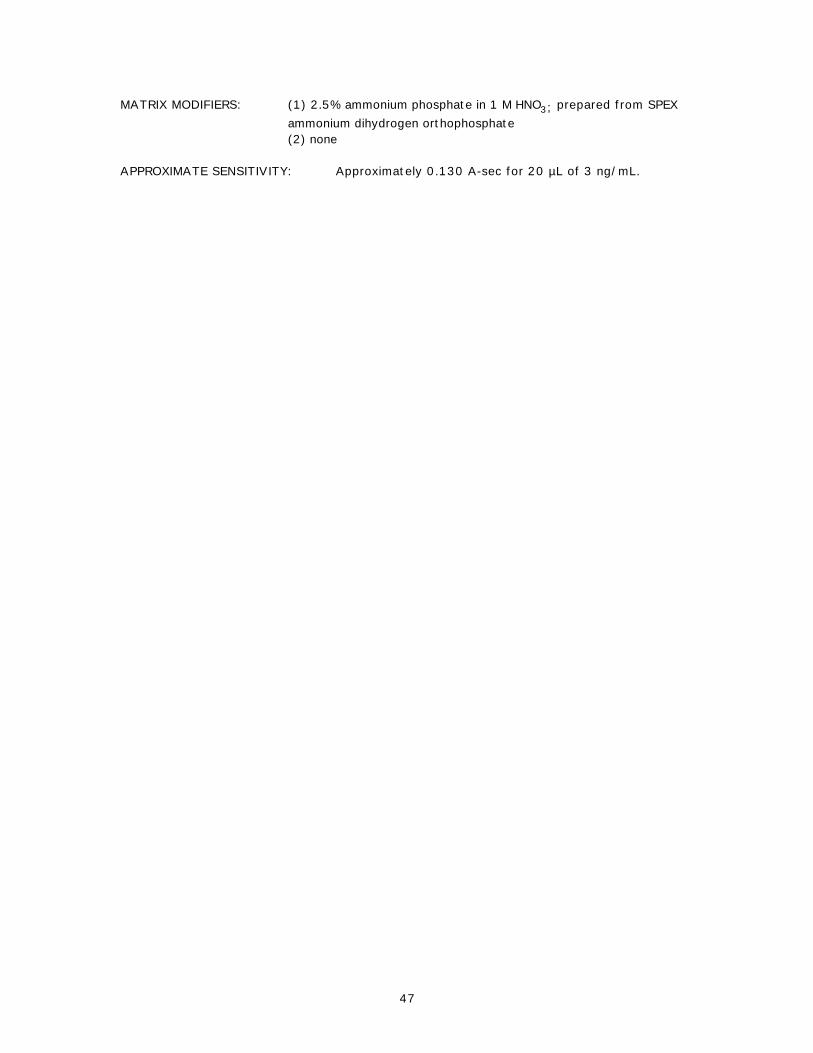
MATRIX MODIFIERS: (1) 2.5% ammonium phosphate in 1 M HNO3; prepared from SPEXammonium dihydrogen orthophosphate(2) none

APPROXIMATE SENSITIVITY: Approximately 0.130 A-sec for 20 µL of 3 ng/mL.

47

7.8. Arsenic


INSTRUMENTATION:

Spectrophotometer: Perkin-Elmer 4100-ZLGraphite furnace: Perkin-Elmer THGAAutosampler: Perkin-Elmer AS 70Printer: Okidata Microline 320


Wavelengths: 193.7 nm197.0 nm (samples with high Al)

Slit width: 0.7 nmLamp: As EDL, 380 WBackground correction: Zeeman effectPeak measurement: Peak areaRead delay: 0 secRead time: 5 secOutput: To printer



FURNACE PROGRAM:


1 120 1 30 2502 150 5 60 2503 800 10 20 2504 2200 0 5 0 *5 2600 1 4 250





48

STANDARDS: 0, 20, 40, and 60 ppb prepared from 1000 ppm Ricca standard in0.2 M HNO3.

MATRIX MODIFIERS (1) 1:1:1 citric acid (2%): Pd (1000 ppm): Ni (4000 ppm)(2) none

APPROXIMATE SENSITIVITY: Approximately 0.100 A-sec for 20 µL of 50 ng/mL at193.7 nm; and 0.050 A-sec at 197.0 nm.

49

7.9. Cadmium


INSTRUMENTATION:



Wavelength: 228.8 nmSlit width: 0.7 nmLamp: Cd EDL, 5 WBackground correction: Zeeman effectPeak measurement: Peak areaRead delay: 0 secRead time: 5 secOutput: To printer



FURNACE PROGRAM:


1 130 10 35 3002 350 10 20 3003 100 1 5 3004 1300 0 5 0 *5 2300 1 4 300





STANDARDS: 0, 1, 2.5, and 4 ppb prepared from 1000 ppm Ricca standard in 0.2M HNO3.

50

MATRIX MODIFIERS: (1) 2% citric acid(2) none

APPROXIMATE SENSITIVITY: Approximately 0.110 A-sec for 10 µL of 1.4 ng/mL.

51

7.10. Chromium


INSTRUMENTATION:



Wavelength: 357.9 nmSlit width: 0.7 nmLamp: Cr HCL, 25 mABackground correction: Zeeman effectPeak measurement: Peak areaRead delay: 0 secRead time: 5 secOutput: To printer



FURNACE PROGRAM:


1 130 10 50 2002 1000 10 20 2003 100 1 5 2004 2400 0 5 0 *5 2500 1 4 300






52

MATRIX MODIFIERS: (1) Dilute NH3, prepared in quartz-distilled water by isothermaldistillation(2) none

APPROXIMATE SENSITIVITY: Approximately 0.160 A-sec with 15 µL of 7 ng/mL.

53

7.11. Copper


INSTRUMENTATION:



Wavelength: 324.8 nmSlit width: 0.7 nmLamp: Cu HCL, 15 mABackground correction: Zeeman effectPeak measurement: Peak areaRead delay: 0 secRead time: 5 secOutput: To printer



FURNACE PROGRAM:


1 110 10 35 2002 500 10 20 2003 100 1 5 2004 1600 0 5 0 *5 2500 1 4 300






54

MATRIX MODIFIERS: (1) Citric acid (2%)(2) none


55

7.12. Nickel


INSTRUMENTATION:



Wavelength: 232 nmSlit width: 0.2 nmLamp: Ni HCL, 25 mABackground correction: Zeeman effectPeak measurement: Peak areaRead delay: 0 secRead time: 5 secOutput: To printer



FURNACE PROGRAM:


1 130 10 40 2002 1000 10 20 2003 100 1 5 2004 2200 0 4 0 *5 2500 1 5 300






56

MATRIX MODIFIERS: (1) 2:2:1 Pd (1000 ppm) : La (1000 ppm) : MgNO3 (2%)(2) none


57

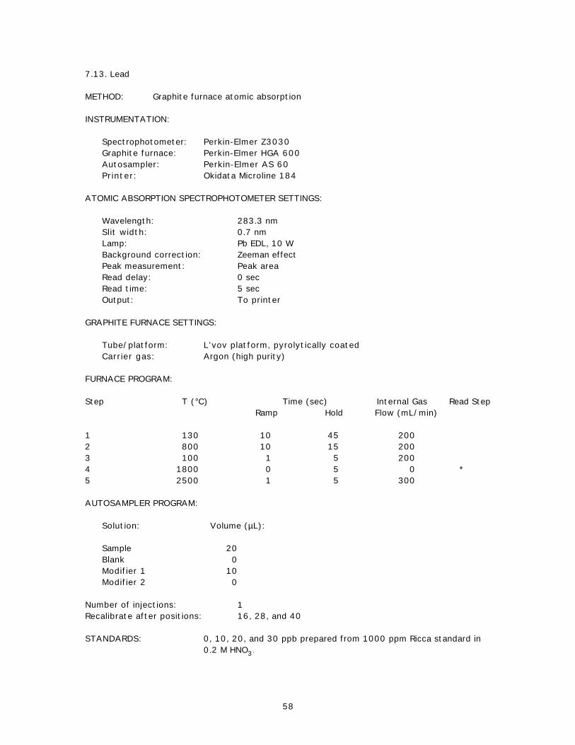
7.13. Lead


INSTRUMENTATION:



Wavelength: 283.3 nmSlit width: 0.7 nmLamp: Pb EDL, 10 WBackground correction: Zeeman effectPeak measurement: Peak areaRead delay: 0 secRead time: 5 secOutput: To printer



FURNACE PROGRAM:


1 130 10 45 2002 800 10 15 2003 100 1 5 2004 1800 0 5 0 *5 2500 1 5 300






58

MATRIX MODIFIERS: (1) 1:1 ammonium phosphate (4%, prepared from ammoniumdihydrogen orthophosphate) and citric acid (2%)(2) none


59

7.14. Selenium


INSTRUMENTATION:



Wavelength: 196.0 nmSlit width: 0.7 nmLamp: Se EDL, 6 WBackground correction: Zeeman effectPeak measurement: Peak areaRead delay: 0 secRead time: 5 secOutput: To printer



FURNACE PROGRAM:


1 130 10 50 2002 900 10 15 2003 100 1 5 2004 2300 0 5 0 *5 2500 1 4 300






60

MATRIX MODIFIERS: (1) 5:3:1 Pd (1000 ppm) : Ni (4000 ppm) : hydroxylaminehydrochloride (2%)(2) none


61

7.15. Tin


INSTRUMENTATION:



Wavelength: 286.3 nmSlit width: 0.7 nmLamp: Sn EDL, 8 WBackground correction: Zeeman effectPeak measurement: Peak areaRead delay: 0 secRead time: 5 secOutput: To printer



FURNACE PROGRAM:


1 130 10 50 2002 800 10 10 2003 100 1 5 2004 2100 0 5 0 *5 2300 1 4 300





STANDARDS: 0, 10, 25, and 50 ppb prepared from 1000 ppm Ricca standard in0.2 M HCl.

62

MATRIX MODIFIERS: (1) 1:1 magnesium nitrate (0.2%) and ammonium phosphate (4%,prepared from ammonium dihydrogen orthophosphate)(2) none


63

7.16. Aluminum

METHOD: Instrumental neutron activation analysis for Al in sediments

INSTRUMENTATION:

TRIGA 1 MW reactorOrtec high-resolution germanium detectorNuclear Data Genie MCA

IRRADIATION CONDITIONS:

Position: PneumaticsNominal neutron flux: 1 x 1013 neutrons/cm2/secLength of irradiation: 30 secCooling period: 15 minPeak measurement: Net peak area using Nuclear Data peak program

COUNTING CONDITIONS:

Counting position: 2-10 cmg-ray peak energy: 1779 KeVCount time: 300 sec

STANDARDS:

Pure element standards: 0.01 g prepared from 1000 ppm Ricca standard.Matrix standards: 0.1 g of: TAMU HS2* , USGS GXR-5, NIST SRM 1646, NRC

BCSS-1, NRC MESS-2.

SAMPLE PREPARATION: Approximately 0.1 g weighed to nearest 0.0001 g into 0.4-dram polyethylene vials.

APPROXIMATE SENSITIVITY: Depends upon background; 100 µg results in approximately1000 counts with associated counting error of 10%; withtypical background and 0.1 g sample size, this correspondsto 0.1% Al.

* TAMU HS2 is a "house" reference sediment standard collected using a box corer in the Mississippi river delta. The sedimentwas washed several times in distilled water to remove dissolved salts, freeze dried, ground with a mortar and pestle, andhomogenized.

64

7.17. Chromium

METHOD: Instrumental neutron activation analysis for Cr in sediments

INSTRUMENTATION:



Position: RotisserieNominal neutron flux: 1 x 1013 neutrons/cm2/secLength of irradiation: 14 hrCooling period: 10 daysPeak measurement: Net peak area using Nuclear Data peak program


Counting position: 10 cmg-ray peak energy: 320.1 KeVCount time: 60 min

STANDARDS:

Pure element standards: 1000 µg prepared from 1000 ppm Ricca standard.Matrix standards: 0.5 g of: TAMU HS2, USGS GXR-5, NIST SRM 1646, NRC

BCSS-1, NRC MESS-2.


APPROXIMATE SENSITIVITY: Depends upon background; 1 µg results in approximately1000 counts with associated counting error of 15%; withtypical background and 0.5 g sample size, this correspondsto 2 ppm Cr.

65

7.18. Iron

METHOD: Instrumental neutron activation analysis for Fe in sediments

INSTRUMENTATION:





Counting position: 10 cmg-ray peak energy: 1099.2 KeVCount time: 60 min

STANDARDS:

Pure element standards: 0.01 g prepared from 1000 ppm Ricca standard.Matrix standards: 0.5 g of: TAMU HS2, USGS GXR-5, NIST SRM 1646, NRC

BCSS-1, NRC MESS-2.


APPROXIMATE SENSITIVITY: Depends upon background; 150 µg results in approximately1000 counts with associated counting error of 10%; withtypical background and 0.5 g sample size, this correspondsto 300 ppm Fe.

66

7.19. Manganese

METHOD: Instrumental neutron activation analysis for Mn in sediments

INSTRUMENTATION:



Position: PneumaticsNominal neutron flux: 1 x 1013 neutrons/cm2/secLength of irradiation: 30 secCooling period: 15 minPeak measurement: Net peak area using Nuclear Data peak program


Counting position: 2-10 cmg-ray peak energy: 846.8 KeVCount time: 300 sec

STANDARDS:

Pure element standards: 1000 µg prepared from 1000 ppm Ricca standard.Matrix standards: 0.1 g of TAMU HS2, USGS GXR-5, NIST SRM 1646, NRC

BCSS-1, NRC MESS-2.


APPROXIMATE SENSITIVITY: Depends upon background: 1 µg results in approximately1000 counts with associated counting error of 10%; withtypical background and 0.1 g sample size, this correspondsto 10 ppm Mn.

67

7.20. Arsenic

METHOD: Instrumental neutron activation analysis for As in tissues

INSTRUMENTATION:

TRIGA 1 MW reactorOrtec high-resolution, high-purity germanium detectorNuclear Data Genie MCA implemented on Digital VAX workstation




Counting position: Variable, depending upon sample activity; normally 10-20 cmGamma-ray peak energy: 559.1 KeVCount time 30-45 min, depending on concentration

STANDARDS:

Pure element standards: 6 µg prepared from 1000 ppm Ricca standardMatrix standards: 0.25 g of: NRC DOLT-2; NRC DORM-2, NIST SRM

1566

SAMPLE PREPARATION: Approximately 0.25 to 0.5 g tissue weighed tonearest 0.0001 g into 0.4 dram polyethylene vial

APPROXIMATE SENSITIVITY: Depends upon background; 0.85 µg, results inapproximately 1000 counts above background withassociated counting error of 10%; with typical backgroundand 0.25 g sample size, this corresponds to 3.4 ppm on adry weight basis.

68

7.21. Chromium

METHOD: Instrumental neutron activation analysis for Cr in tissues

INSTRUMENTATION:




COUNTING CONDITIONS.

Counting position: 1-10 cmGamma-ray peak energy: 320.1 KeVCount time: 75 min

STANDARDS:

Pure element standards: 5 -g prepared from 1000 ppm Ricca standardMatrix standards: 0.25 g of: NRC DOLT-2; NRC DORM-2, NIST SRM

1566a.


APPROXIMATE SENSITIVITY: Depends upon background; 0.25 µg, results inapproximately 1000 counts above background withassociated counting error of 10%; with typicalbackground and 0.25 g sample size, thiscorresponds to 1.0 ppm Cr on a dry weight basis.

69

7.22. Iron

METHOD: Instrumental neutron activation analysis for Fe in tissues

INSTRUMENTATION:



Position: RotisserieNominal neutron flux: 1 x 1013 neutrons/cm2/secLength of irradiation: 14hrCooling period: 10 daysPeak measurement: Net peak area using Nuclear Data peak program



STANDARDS:


1566a

SAMPLE PREPARATION: Approximately 0.25 to 0.5 g tissue weighed to nearest0.0001 g into dram polyethylene vial

APPROXIMATE SENSITIVITY: Depends upon background; 36 µg, results in approximately1000 counts above background with associated countingerror of 10%; with typical background and 0.25 samplesize, this corresponds to 145 ppm on a dry weight basis.

70

7.23. Selenium

METHOD: Instrumental neutron activation analysis for Se in tissues

INSTRUMENTATION:






STANDARDS:

Pure element standards 6 µg prepared from 1000 ppm Ricca standardMatrix standards: 0.25 g of: NRC DOLT-2; NRC DORM-2, NIST SRM

1566a


APPROXIMATE SENSITIVITY: Depends upon background; 0.22 µg, results inapproximately 1000 counts above backgroundassociated counting error of 10%; with typicalbackground and 0.25 g sample size, thiscorresponds to 0.87 ppm on a dry weight basis.

71

7.24. Silver

METHOD: Instrumental neutron activation analysis for Ag in tissues

INSTRUMENTATION:






STANDARDS:


1566a


APPROXIMATE SENSITIVITY: Depends upon background; 0.14 µg, results inapproximately 1000 counts above background withassociated counting error of 10%; with typicalbackground and 0.25 g sample size, thiscorresponds to 0.55 ppm Ag on a dry weight basis.

72

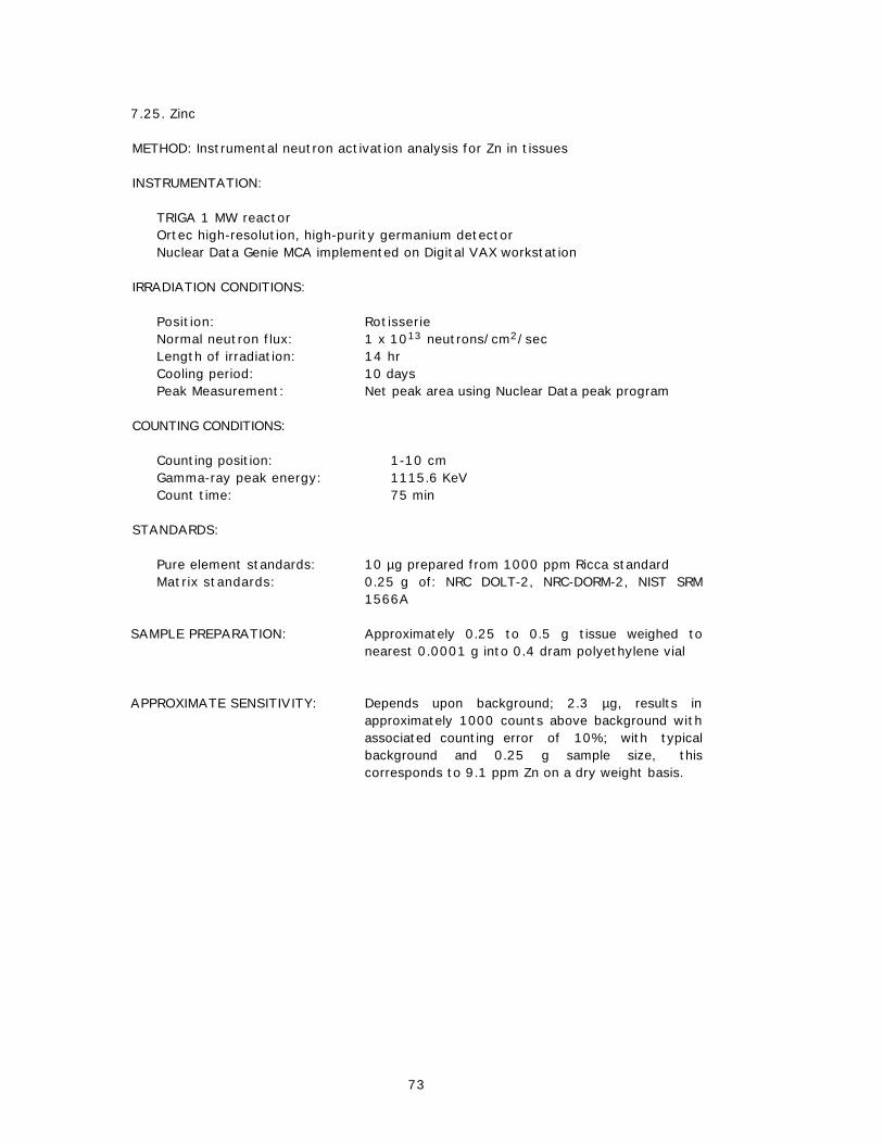
7.25. Zinc

METHOD: Instrumental neutron activation analysis for Zn in tissues

INSTRUMENTATION:



Position: RotisserieNormal neutron flux: 1 x 1013 neutrons/cm2/secLength of irradiation: 14 hrCooling period: 10 daysPeak Measurement: Net peak area using Nuclear Data peak program



STANDARDS:

Pure element standards: 10 µg prepared from 1000 ppm Ricca standardMatrix standards: 0.25 g of: NRC DOLT-2, NRC-DORM-2, NIST SRM

1566A


APPROXIMATE SENSITIVITY: Depends upon background; 2.3 µg, results inapproximately 1000 counts above background withassociated counting error of 10%; with typicalbackground and 0.25 g sample size, thiscorresponds to 9.1 ppm Zn on a dry weight basis.

73

Analysis of Marine Sediment and Bivalve Tissueby X-Ray Fluorescence, Atomic Absorption and Inductively Coupled

Plasma Mass Spectrometry

E. Crecelius, C. Apts, L. Bingler, J. Brandenberger, M. Deuth, S. Kiesser, and R. Sanders *

Battelle/Marine Sciences Laboratory1529 West Sequim Bay Rd.

Sequim, Washington

ABSTRACT

Analytical chemistry techniques including atomic absorption spectrophotometry,inductively coupled plasma mass spectrometry (ICP-MS) and energy dispersive x-rayfluorescence (XRF) have been applied to the analysis of 17 elements in aquatic sedimentand bivalve tissue in support of the NOAA NS&T Program. Complete acid digestion ofsamples at elevated pressure and temperature in a sealed Teflon container minimizescontamination and loss of elements. Multi-elemental techniques such as ICP-MS and XRFprovide sensitive, accurate, and precise results for a variety of elements at areasonable cost.

1. INTRODUCTION

Methods used for analysis of 17 metals in estuarine sediments and tissues were developed aspart of the Mussel Watch Project of the National Status and Trends (NS&T) Program. The totaldigestion procedure used for sediments, without loss of volatile elements, was developed byTaylor and Presley (this volume) at Texas A&M University (TAMU). The digestion procedurefor tissues was a combination of HCl and HNO3. Metals were analyzed predominantly bygraphite furnace atomic absorption (GFAA) spectrometry and x-ray fluorescence (XRF).Mercury was analyzed by cold vapor atomic absorption (CVAA). Selected metals weredetermined by inductively-coupled plasma mass spectrometry (ICP-MS). The primaryobjective in developing each instrumental method was to keep the method as simple andstraightforward as possible while producing acceptable accuracy and precision.

It is expected that users of the instrumental methods described below will modify certainparameters to suit their particular instrumentation and equipment due to variations inperformance between instruments. Such variations are caused by differences in furnacecalibration, lamp intensities, nebulizer characteristics, and other parameters.


2.1. Instrumentation

Perkin-Elmer model Z/5000 spectrophotometer. Perkin-Elmer, Norwalk, CT.

Dual lamp EDL power supplyModel 500 graphite furnace atomizer with Zeeman background correction systemModel 3600 data terminalModel AS40 autosampler

* KLM Analytical, 2000 Logston Blvd., Richland, WA 99352.

74

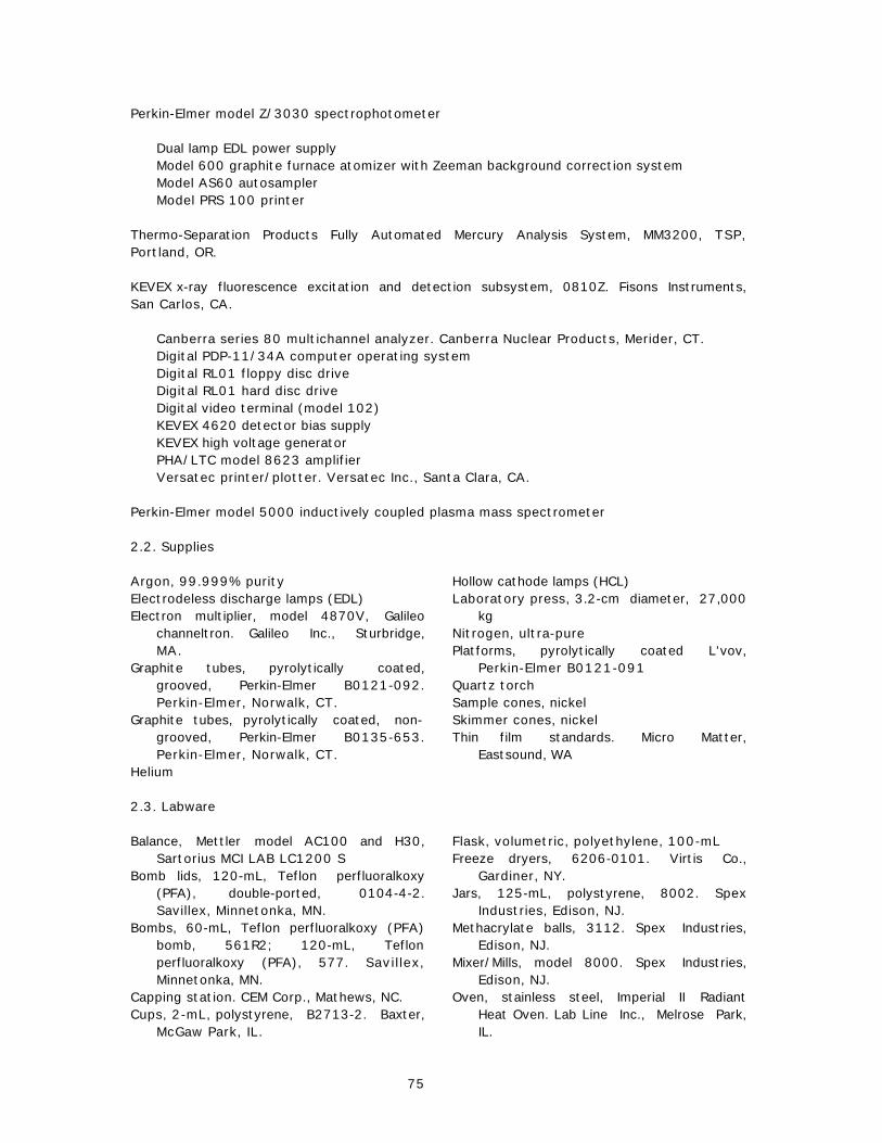
Perkin-Elmer model Z/3030 spectrophotometer

Dual lamp EDL power supplyModel 600 graphite furnace atomizer with Zeeman background correction systemModel AS60 autosamplerModel PRS 100 printer

Thermo-Separation Products Fully Automated Mercury Analysis System, MM3200, TSP,Portland, OR.

KEVEX x-ray fluorescence excitation and detection subsystem, 0810Z. Fisons Instruments,San Carlos, CA.

Canberra series 80 multichannel analyzer. Canberra Nuclear Products, Merider, CT.Digital PDP-11/34A computer operating systemDigital RL01 floppy disc driveDigital RL01 hard disc driveDigital video terminal (model 102)KEVEX 4620 detector bias supplyKEVEX high voltage generatorPHA/LTC model 8623 amplifierVersatec printer/plotter. Versatec Inc., Santa Clara, CA.

Perkin-Elmer model 5000 inductively coupled plasma mass spectrometer

2.2. Supplies

Argon, 99.999% purity Hollow cathode lamps (HCL)Electrodeless discharge lamps (EDL) Laboratory press, 3.2-cm diameter, 27,000

kgElectron multiplier, model 4870V, Galileochanneltron. Galileo Inc., Sturbridge,MA.

Nitrogen, ultra-purePlatforms, pyrolytically coated L'vov,

Perkin-Elmer B0121-091Graphite tubes, pyrolytically coated,grooved, Perkin-Elmer B0121-092.Perkin-Elmer, Norwalk, CT.

Quartz torchSample cones, nickel

Graphite tubes, pyrolytically coated, non-grooved, Perkin-Elmer B0135-653.Perkin-Elmer, Norwalk, CT.

Skimmer cones, nickelThin film standards. Micro Matter,

Eastsound, WAHelium

2.3. Labware

Balance, Mettler model AC100 and H30,Sartorius MCI LAB LC1200 S

Flask, volumetric, polyethylene, 100-mLFreeze dryers, 6206-0101. Virtis Co.,

Gardiner, NY.Bomb lids, 120-mL, Teflon perfluoralkoxy(PFA), double-ported, 0104-4-2.Savillex, Minnetonka, MN.

Jars, 125-mL, polystyrene, 8002. SpexIndustries, Edison, NJ.

Bombs, 60-mL, Teflon perfluoralkoxy (PFA)bomb, 561R2; 120-mL, Teflonperfluoralkoxy (PFA), 577. Savillex,Minnetonka, MN.

Methacrylate balls, 3112. Spex Industries,Edison, NJ.

Mixer/Mills, model 8000. Spex Industries,Edison, NJ.

Capping station. CEM Corp., Mathews, NC. Oven, stainless steel, Imperial II RadiantHeat Oven. Lab Line Inc., Melrose Park,IL.

Cups, 2-mL, polystyrene, B2713-2. Baxter,McGaw Park, IL.

75

Pipettes, macro and micro Teflon tubing, 1-mm i.d.Polyethylene tubing, 7420. Clay Adams Co.,

Parsippany, NJ.Vials, 20-mL, polyethylene, threaded, with

screw caps, Kimble 66022-241Spatulas Vials, dry grinding, ceramic, 8003. Spex

Industries, Edison, NJ.Stopwatch or timer

Polyethylene vials were cleaned by soaking for five days in 5% HNO3, at room temperature,rinsed with deionized water and dried in Class 100 laminar flow hoods. All other plastic warewas soaked for three days in 10% HNO3 at room temperature, rinsed with deionized water,and dried as above. Teflon bombs were soaked for two days in 50% concentrated HNO3.

2.4. Reagents

All reagents are ultrapure grades except where so designated.

Ammonium dihydrogen phosphate (NH4H2PO4)[7722-76-1], Ultrex 7-9431. J. T.Baker, Phillipsburg, NJ.

Nickel nitrate [Ni(NO3)2 . 6H2O] [13478-00-

7], solid, Puratonic Grade. JohnsonMatthey Chemicals, West Chester, PA.

Ammonium nitrate (NH4NO3) [6484-52-2],,solid, reagent grade, 729-1. J. T. Baker,Phillipsburg, NJ.

Nitric acid (HNO3) [7697-37-2], concen-trated (70%), Instra-analyzed, 9598-33. J. T. Baker, Phillipsburg, NJ.

Ascorbic acid (C6H8O6) [50-81-7], solid,reagent grade, 581-5. J. T. Baker,Phillipsburg, NJ.

Perchloric acid (HClO4) [7601-90-3],concentrated (70%), 230. G. FrederickSmith, Columbus, OH.

Atomic absorption standards, 1000 µg/mL.High-Purity Standards, Inc., Charleston,SC.

Soda lime [variable mixture of NaOH andCaO/Ca(OH)2] [8006-28-8], 4-8 mesh,used as acid fume trap in CVAA, 3448-01. J. T. Baker, Phillipsburg, NJ.Hydrochloric acid (HCl) [7647-01-0],

concentrated (37%), Instra-analyzed,9530-33. J. T. Baker, Phillipsburg, NJ.

Stannous chloride (SnCl2 . 2H2O) [10025-69-1], 3980-01. J. T. Baker,Phillipsburg, NJ.

Hydrofluoric acid (HF) [7664-39-3], Instra-analyzed, 9563-01. J. T. Baker,Phillipsburg, NJ.

Sulfuric acid (H2SO4) [7664-93-9], con-centrated (98%), Instra-analyzed,9673-33. J. T. Baker, Phillipsburg, NJ.

Magnesium nitrate [Mg(NO3)2. 6H2O]

[13446-18-9], solid, Puratonic Grade.Johnson Matthey Chemicals, WestChester, PA.

Water, deionized, 10 megohm-cm re-sistivity.

2.5. Solvents and matrix modifiers

Ammonium phosphate: 2%, monobasic, 2 g of NH4H2PO4 and 0.200 g of Mg(NO3)2 per literof deionized water.

Ammonium phosphate: 4%, monobasic, 4 g NH4H2PO4 and 13 g NH4NO3 diluted to 100 mLwith deionized water.

Magnesium nitrate solution: 250 mg/L of deionized water.0.10 M Nickel nitrate: 2.91 g Ni(NO3)2

.6H2O in 100 mL of deionized water.Sulfuric acid modifier solution: Dilute 1 mL of concentrated sulfuric acid to 99 mL with

deionized water and add 10 µL of 0.1 M Ni(NO3)2.6H2O.

76

3. SAMPLE TREATMENT

3.1. Drying and homogenization

3.1.1. Sediments

Sediments were obtained with a grab sampler that collects the top 2 cm of surface sediment.Sample aliquots were weighed, freeze-dried for approximately 5 days to constant weight in125-mL polystyrene Spex jars in a freeze dryer, and reweighed to determine percent dryweight. Approximately 3 g were ground for 5 min using a Spex ceramic ball mill. Aliquots of0.5 g were used for X-ray fluorescence, or digested for atomic absorption or ICP-MSanalysis.

3.1.2. Tissues

Bivalves were hand-collected and shucked at the lab. Tissues were freeze-dried in Spex jarsand homogenized using methacrylate balls in a Spex mixer/mill.

3.2. Digestion

Battelle used minor modifications of the total digestion techniques for sediments developed byTaylor and Presley (this volume). Tissues were digested with a mixture of HCl and HNO3

which has been shown to provide much better recovery of Ag than HNO3 or HNO3 and HClO4

(Crecelius and Daskalakis, 1994; Daskalakis et al., 1997).

Two reagent blanks and three standard reference material samples were included in eachanalytical string of 50 samples. Reagent blanks contained no sediment or tissue and wereprocessed like the samples.

3.2.1. Sediments

Approximately 200 ± 7 mg of homogenized ground dried sediment was weighed into a tared60-mL Teflon digestion bomb. One mL of 4:1 HNO3/HClO4 was added to each bomb and thelid tightened at the capping station.

The bombs were heated in the oven at 130 ± 10 °C for 4 hr and allowed to cool.

Three mL of concentrated HF were added to each bomb, rinsing the walls of the bomb toinsure that all solids were washed down into the acid mixture. The lid was tightened at thecapping station.


The bombs were opened and the digestates diluted to approximately 20 mL with deionizedwater.

The solutions were weighed in the Teflon bombs and the volume calculated using a densityfactor of 1.05 g/mL.

The contents of each bomb were transferred quantitatively to a 20-mL polyethylenescrew-cap vial for storage prior to analysis.

77

Digestates were analyzed directly by GFAA or CVAA. Before analysis by ICP-MS, a 10-mLaliquot was transferred to a Teflon bomb and dried slowly, uncovered, on a hot plate (203 °C)in a perchloric acid hood to eliminate chloride and fluoride. White fumes were indicative ofsuccessful elimination of these elements. The dried digestate was dissolved in 1 mL of 10%HNO3 and heated again to dryness. The dried digestate was dissolved again with 1 mL of 10%HNO3 and 9 mL of deionized water.

3.2.2. Tissues

Approximately 500 ± 15 mg of homogenized, dried tissue was weighed into a tared 60-mLTeflon digestion bomb. Five mL of HCl and 3.5 mL of HNO3 were added to each bomb and thelid screwed on but not tightened.

The bombs were placed in a cold water bath in an acid hood and the water bath was heatedslowly to 60 ± 3 °C. The total heating time was 3 to 4 hr.

The bombs were allowed to cool. The lids were tightened at the capping station.


The bombs were opened and the digestates diluted to approximately 20 mL with deionizedwater.

The solutions were weighed in the Teflon bombs and the volume calculated using a densityfactor of 1.09 g/mL.

Digestates were analyzed directly by GFAA and CVAA, or diluted 10:1 for ICP-MS analysis.

4. CALIBRATION

Calibration standards were prepared by serial dilution of commercially available atomicabsorption standards using class-A glass pipettes, volumetric flasks, and 10% HNO3. Somemetals, such as Sb and Sn, required use of a different acid diluent. Final working standardswere prepared in 1% HNO3 or the appropriate acid diluent, using micropipettes and glassvolumetric flasks. The element concentrations in each standard should be sufficient to coverthe appropriate range of sample concentrations and produce good measurement precision andaccurately define the slope of the response curve. Concentrations of commercial standardswere verified by comparison with National Institute of Standards and Technology (NIST)spectrophotometric standards.

5. SPECTRAL INTERFERENCES

Spectral interferences may be minimized by sample dilution, use of an alternate analytewavelength, or selective volatilization of the analyte. Non-spectral interferences may bedetected and compensated for using the method of standard additions. Matrix modifiers thatwere used include Mg(NO3)2, NH4H2PO4, Ni(NO3)2, and H2SO4. Their specific use is describedin the instrumental analysis section for each element.

78

6. CALCULATIONS

6.1. Graphite furnace and ICP-MS

Sample concentrations were determined from calibration results and from the dilution factorsusing the following equation:

Concentration (µg/g dry wt) = (SA - B A) m SV

1000 (SDW) (DF)

where SA was the sample absorbance or intensity value, BA was the procedural blankabsorbance or intensity value, m was the slope of standard addition calibration line, SV wasthe sample volume, SDW was the sample dry weight in grams, and DF was the dilution factor.

6.2. Cold vapor atomic absorption

Sample concentrations were determined from calibration results and from the dilution factorsinvolved in instrumental analysis and sample digestion according to the following equation:

Concentration (µg/g dry wt) = (SA - B A) m SV

1000 (SDW) (DF)

where SA was the sample absorbance value, BA was the procedural blank absorbance value, mwas the slope of the calibration line, SV was the sample volume, SDW was the sample dryweight in grams, and DF was the dilution factor.

6.3. X-ray fluorescence

This procedure used energy dispersive x-ray fluorescence spectroscopy to quantify elementalconcentrations in sediment and tissue samples (Nielson et al ., 1982). The backscatter/fundamental parameter approach using the SAP3 computer code incorporated thin filmstandards and scattering rations to produce matrix corrections (Nielson and Sanders, 1982).

Thin film standards were used for the determination of intensity in count/min/µg(element)/cm2 versus element energy in KeV. Thin film standards produced by vapor depositof the elements on Mylar or polycarbonate substrate were purchased from Micro Matter ofEastsound, WA. These standards were traceable to the U.S. National Institute of Standards andTechnology.

The peak analysis and elemental concentration sections of the computer program (SAP3) usedarrays of fundamental physical parameters of x-ray energies, mass adsorption coefficients,cross sections, fluorescence yields, absorption edge, and jump ratios to perform the matrixcorrections for relating net peak intensities to element concentrations. These arrays wereread into the computer from a disc file when the program was initiated. Each excitation sourcehad its own unique disc file or library. Thin film sensitivities or calibration factors of thespectrometer using the intended excitation source was also part of the library.

79

7. CONCLUSIONS

A variety of analytical instruments provided the optimum method for the analysis of 17elements in sediment and bivalve tissue. The advantage of XRF was that the sample did notrequire digestion but was analyzed as a dry powder. Crustal elements such as Al, Cr, Fe, Ni,and Si, that are difficult to dissolve from sediment, could be quantified by XRF. Also, Se andAs can be difficult to quantify in tissue digestates by ICP-MS but were quantified easier usingXRF. ICP-MS had the advantage of simultaneous analysis of many elements with detectionlimits much lower than the XRF and similar to those of GFAA. Elements that were particularlysensitive and relatively interference free by ICP-MS include Al, Cr, Ni, Ag, Cd, Sn, Sb, Pb,and Tl. Cold vapor atomic absorption is a very sensitive and reliable technique for Hg analysis.Care must be taken to avoid leakage at high pressure or Hg can be lost during digestion. Withthe use of the sealed Teflon digestion vessel, mercury could be analyzed from the samedigestion as the other metals (Al, Cr, Ni, Ag, Cd, Sn, Sb, Pb, and Tl).

The advantage of freeze drying both sediment and tissue was that the dry material was easilyground or homogenized. No Hg loss occurred during freeze drying. Sediment digestatesreceived special treatment to remove silicon, fluoride and perchloric acid before analysis byICP-MS. Analysis by GFAA requires matrix modifiers and standardization of the instrument bymethod of addition to the sample matrix to provide accurate results.

8. REFERENCES

Crecelius, E. A., and K. D. Daskalakis (1994) Analysis of silver in mussels and oysters byinductively coupled plasma mass spectrometry (ICPMS). Proc., Second Internatl. Conf.,Transport, Fate and Effects of Silver in the Environment. A. W. Andren and T. W. Bober (eds.).September 11-13, 1994. Madison, WI. 157-9.

Daskalakis, K. D., T. P. O'Connor, and E. A. Crecelius (1997) Evaluation of digestionprocedures for determining silver in mussels and oysters. Environ. Sci. Technol., 31:2303-2306).

Nielson, K. K., and R. W. Sanders (1982) The SAP3 computer program for quantitative multi-element analysis by energy-dispersive x-ray fluorescence. PNL-4173, Battelle PacificNorthwest Laboratory, Richland, WA. 120 pp.

Nielson, K. K., R. W. Sanders, and J. C. Evans (1982) Analysis of steels by energy-dispersivex-ray fluorescence with fundamental parameters. Anal. Chem., 54(11):1782-6.

Patterson, K. Y., C. Veillon, and H. M. Kingston (1988) Microwave digestion of biologicalsamples. In: Introduction to Microwave Sample Preparation. H. M. Kingston and L. B. Jassie(eds.). 155-66. ACS Professional Reference Book, American Chemical Society, Washington,DC.

80

9. INSTRUMENTAL ANALYSIS

9.1. Atomic absorption spectrometry

9.1.1. Aluminum

Graphite furnace atomic absorption for tissue


DIGEST MATRIX: ~15% 4:1 HNO3:HClO4 by volume.

INSTRUMENT SETTINGS:

Wavelength: 309.3 nmLamp: HCL, 25 ma (Perkin-Elmer 0303-6009)Tube: Non-platform, pyrolytically coatedCarrier gas: ArgonSlit width: 0.7Background correction: ZeemanSignal mode: Peak heightScale expansion: NoneRead time: 5 secOutput: Recorded from spectrophotometer display

FURNACE PROGRAM:

Step T (°C) Time (sec) Internal GasRamp Hold Flow (mL/min)

Dry 1 80 9 1 300Dry 2 140 45 5 300Dry 3 250 20 5 300Char 1600 45 25 300Atomize 2300 0 4 50Cleanout 2650 1 3 300Cool 20 1 10 300

STANDARDS: Addition calibration using 22.2, 43.5, and 83.3 µg/L Al to CRMDOLT-1 tissue digestate. Method of standard addition.

TYPICAL SENSITIVITY: Absorbance is approximately 0.100 for 0.4 µg Al standard.

CALIBRATION: Peak height versus concentration of standards used to compute theslope, intercept, and correlation coefficient of calibration lineusing linear, least-squares regression.

INJECTION VOLUME: 5 µL

MATRIX MODIFIER: 5 µL of 2% NH4H2PO4.

81

9.1.2. Chromium





Wavelength: 357.9 nmLamp: HCL, 25 ma (Perkin-Elmer 0303-6021)Tube: Pyro, non-platformCarrier gas: ArgonSlit width: 0.7Background correction: ZeemanSignal mode: Peak heightScale expansion: NoneRead time: 5 secOutput: Recorded from spectrophotometer display

FURNACE PROGRAM:



STANDARDS: Method of standard addition calibration using 20.0, 33.3, and 66.7µg/L Cr to CRM DOLT-1 tissue digestate.

TYPICAL SENSITIVITY: Absorbance is approximately 0.200 for 0.165 µg Cr standard.

CALIBRATION: Peak height versus concentration of standards used to compute theslope, intercept, and correlation coefficient of calibration lineusing linear, least-squares regression.


MATRIX MODIFICATION: 5 µL of 250 mg/L Mg as Mg(NO3)2.

82

9.1.3. Nickel

Graphite furnace atomic absorption for tissues

METHOD: Graphite Furnace Atomic Absorption



Wavelength: 232.0 nmLamp: HCL, 35 ma (Perkin-Elmer 0303-6047)Tube: Pyro, non-platformCarrier gas: ArgonSlit width: 0.2Background correction: ZeemanSignal mode: Peak heightScale expansion: NoneRead time: 5 secOutput: To printer

FURNACE PROGRAM:



STANDARDS: Method of standard addition calibration using 24.39, 47.62, and90.91 µg/L Ni to CRM DOLT-1 digestate.

TYPICAL SENSITIVITY: Absorbance is approximately 0.100 for 0.6 µg Ni standard.

CALIBRATION: Peak height of standard versus concentration of standard. Computethe slope, intercept, and correlation coefficient using linear,least-squares regression.


MATRIX MODIFICATION: 5 µL of 2% NH4H2PO4.

MODIFIER VOLUME: 5 µL

83

9.1.4. Selenium

Graphite furnace atomic absorption for sediment


DIGEST MATRIX: ~4% 4:1 HNO3:HClO4 + 12% HF by volume.


Wavelength: 195.9 nmLamp: EDL, 6 watts (Perkin-Elmer 0303-6262)Tube: L’vov, pyro coatedCarrier gas: ArgonSlit width: 2.0Background correction: ZeemanSignal mode: Peak heightScale expansion: NoneRead time: 5 secOutput: Recorded from spectrophotometer display

FURNACE PROGRAM:



STANDARDS: Method of standard addition calibration using 47.6, 90.9, and130.4 µg/L Se to CRM MESS-1 sediment digestate.

TYPICAL SENSITIVITY: Absorbance is approximately 0.100 for 1.0 µg Se standard.



MATRIX MODIFICATION: 10 µL of 0.1 M Ni(NO3)2.

84

9.1.5. Silver

9.1.5.1. Graphite furnace atomic absorption for tissue




Wavelength: 327.9 nmLamp: HCL, 12 ma (Perkin-Elmer 0303-6064)Tube: L’vov, pyro coatedCarrier gas: ArgonSlit width: 0.7Background correction: ZeemanSignal mode: Peak heightScale expansion: NoneRead time: 4 secOutput: To printer

FURNACE PROGRAM:



STANDARDS: Addition calibration using 0.99, 1.96, and 4.76 µg/L Ag to CRMDOLT-1 tissue digestate.

TYPICAL SENSITIVITY: Absorbance is approximately 0.100 for 0.03 µg Ag standard.




85

Silver

9.1.5.2. Graphite furnace atomic absorption for sediment


DIGEST MATRIX: ~4% 4:1 HNO3:HClO4 +12% HF by volume.


Wavelength: 327.9 nmLamp: HCL, 12 ma (Perkin-Elmer 0303-6064)Tube: L’vov, pyro coatedCarrier gas: ArgonSlit width: 0.7Background correction: ZeemanSignal mode: Peak heightScale expansion: NoneRead time: 4 secOutput: To printer

FURNACE PROGRAM:



STANDARDS: Addition calibration using 2.44, 4.76, and 9.09 µg/L Ag to SRM1646 sediment digestate.

TYPICAL SENSITIVITY: Absorbance is approximately 0.120 for 0.05 µg Ag standard.




86

9.1.6. Cadmium

9.1.6.1. Graphite furnace atomic absorption for tissue




Wavelength: 228.9 nmLamp: EDL, 5 watts (Perkin-Elmer 0303-60216)Tube: L’vov, pyro coatedCarrier gas: ArgonSlit width: 0.7Background correction: ZeemanSignal mode: Peak areaScale expansion: NoneRead time: 4 secOutput: To printer

FURNACE PROGRAM:



STANDARDS: Addition calibration using 0.96, 2.37, and 4.62 µg/L Cd to SRM1566a tissue digestate.

TYPICAL SENSITIVITY: Absorbance is approximately 0.100 for 0.02 µg Cd standard.

CALIBRATION: Peak area of standard versus concentration of standard. Computethe slope, intercept and correlation coefficient using linear, least-squares regression.



87

Cadmium

9.1.6.2. Graphite furnace atomic absorption for sediment


DIGEST MATRIX: ~4% 4:1 HNO3:HClO4 + 12% HF by volume.


Wavelength: 228.8 nmLamp: EDL, 5 watts (Perkin-Elmer 0303-6216)Tube: L’vov, pyro coatedCarrier gas: ArgonSlit width: 0.7Background correction: ZeemanSignal mode: Peak areaScale expansion: NoneRead time: 4 secOutput: To printer

FURNACE PROGRAM:



STANDARDS: Addition calibration using 0.90, 2.22, and 4.35 µg/L Cd to SRM1646 sediment digestate.

TYPICAL SENSITIVITY: Absorbance is approximately 0.100 for 0.015 µg Cd standard.

CALIBRATION: Peak area of standard versus concentration of standard. Computethe slope, intercept, and correlation coefficient using linear,least-squares regression.



88

9.1.7. Mercury

Cold vapor/gold foil amalgam for tissue or sediment

METHOD: Cold vapor/gold foil amalgam

DIGEST MATRIX: ~25% 5:3.5 HCl and HNO3 by volume for tissues.

~4% 4:1 HNO3 and HClO4 + 12% HF by volume for sediments.


Reaction volume: 0.020 -1 mLDiluent: 3% HNO3

Carrier Gas: ArFlow rate: 200 mL/minScale expansion: Attenuation - mid-rangeIntegration time: 5 minOutput: Peak integrated by system software

REDUCTANT: 2% SnCl2 in 10% HCl

STANDARDS: 0.5, 1.25, 5, 7.5, and 12.5 µg/L made in 3% HCl using HighPurity standards.

TYPICAL SENSITIVITY: 0.001 µg/g Hg.

CALIBRATION: Instrument read-out is in peak area and input is in ng Hg, socalibration curve is based on Hg input versus Hg output reading.The slope, intercept, and correlation coefficient are calculatedusing linear, least-squares regression.

INJECTION VOLUME: 1 to 5 mL

REDUCTANT VOLUME: 2.5 mL

MATRIX MODIFICATION: None

89

9.1.8. Lead





Wavelength: 283.3 nmLamp: EDL, 5 ma (Perkin-Elmer 0303-6039)Tube: L’vov, coatedCarrier gas: ArgonSlit width: 0.7Background correction: ZeemanSignal mode: Peak heightScale expansion: NoneRead time: 5 secOutput: Recorded from Spectrophotometer display

FURNACE PROGRAM:



STANDARDS: Method of standard addition calibration at 9.9, 19.6, and 24.4µg/L Pb to CRM DOLT-1 tissue digestate.

TYPICAL SENSITIVITY: Absorbance is approximately 0.160 for 0.25 µg Pb standard.




90

9.2. Inductively coupled plasma mass spectrometry

Silver, aluminum, chromium, cadmium, nickel, lead, antimony, and tin in sediments or tissues

METHOD: Inductively coupled plasma mass spectrometry

DIGEST MATRIX: 1 to 10 dilution of digestate with deionized water plus 0.1 mL of 1ppm In standard.

INSTRUMENT SETTINGS: Instrument settings change on a daily basis as sensitivity isoptimized. This is especially true of lens settings. The followinggives general ranges on parameters that remain relativelyconstant in day-to-day operation:

Power: 1250-1500 wattsCoolant flow: 13-14 L/min.Auxiliary flow: 0.5-1.0 L/min.Nebulizer flow: 0.85-1.0 L/min.EM voltage: 2000-3000 voltsSample uptake: 0.5-1.5 mL/min.Integration method: Constant areaIntegration area: 0.8Background counts: 35Dead time: 40 nsecQuad slew factor: 0.10

PROCEDURE:

Element menu: tissue2Mass range: 25.98 to 212.05 amuNumber of channels: 2048Number of sweeps: 100Dwell time: 320 µsecCollector type: pulseInternal standards: InSkipped mass regions: 28.00 - 43.00, 63.00 - 105.00, 125.00 - 200

STANDARDS: Appropriate calibration standards (representative of sampleconcentration) are prepared from dilutions of NIST single- and/ormulti-element standards. Other reference materials (NIST orsecond party single/multi-element standards) are used as checkstandards. Method of standard addition can be used to produceinstrumental response curve.

TYPICAL SENSITIVITY: Sensitivity is approximately 5 x 104 million counts per sec perppm for In115.

CALIBRATION: Constant area integration (using 0.8 of total peak) versusconcentration of standard. Compute the slope, intercept, andcorrelation coefficient using linear, least-squares regression.

91

9.3. X-Ray fluorescence

Elements in sediment: Al, As, Cr, Cu, Fe, Mn, Ni, Pb, Si, and Zn.Elements in tissue: As, Cu, Fe, Mn, Se, Si, and Zn.

METHOD: X-ray fluorescence

Sample preparation: 0.5 g dried and homogenized sediment or tissue pressed in a pellet,2 cm in diameter.


Gain: PHA/LTC for Series 80 MCASecondary target: ZrTarget gain: 25 eV/channelResolution: 182 eV at 6.4 KeVTiming counter: 12 µsecBias: -1000 VLive time: 1500 secDead time: < 40%Tungsten tube voltage: 40 VTube current: 20 milliamps

92

ORGANIC ANALYSES

93

Extraction and Clean-Up of Sediments for Trace Organic Analysis



ABSTRACT

Measurement of organic contaminants, such as polychlorinated biphenyls, polynucleararomatic hydrocarbons, and chlorinated pesticides, in soil/sediment require theisolation of these contaminants from the matrices. An aliquot of the homogenizedsediment sample was chemically dried with sodium sulfate and extracted withdichloromethane using a Soxhlet apparatus. The extract was concentrated and purifiedusing silica gel/alumina column chromatography before instrumental analysis. Qualitycontrol samples were processed with each batch of samples in a manner identical to thesamples.

1. INTRODUCTION

Assessment of the environmental concentrations of polynuclear aromatic hydrocarbons (PAHs),chlorinated pesticides and polychlorinated biphenyls (PCBs) requires their measurement insediments at trace levels (parts per billion to parts per trillion).

Ten to thirty grams of chemically-dried sediment was Soxhlet extracted with dichloromethane.The extract was concentrated and purified using silica gel/alumina column chromatography toremove matrix interferences.


2.1. Sample collection

Sediment was collected and stored in precleaned glass jars and stored frozen (-20 °C).

2.2. Sample preservation and storage

Sediment samples were shipped frozen to the laboratory and stored at -20 °C until analysis.After subsampling, excess sample was archived at -20 °C in the dark. Extracts were stored inthe dark at or below 4 °C.

3. INTERFERENCES

Method interferences may be caused by contaminants in solvents, reagents, glassware, andother sample processing hardware, and lead to false positives during instrumental analysis. Allmaterials used in this method were routinely demonstrated to be free from interferences byprocessing procedural blanks identical to samples (one blank per 20 samples or each batchwhichever is more frequent).

Matrix interferences result from co-extraction of compounds other than the analytes ofinterest. Elemental sulfur and naturally occurring lipids can cause interferences in the analysis

94

of sediment extracts. Silica gel/alumina cleanup with activated copper was used to removeinterfering materials from the sample prior to analysis.



Glassware was cleaned by washing with Micro cleaning solution and rinsing with water. Theglassware was then combusted in a muffle furnace at 440 °C for at least 4 hr. Solvent rinsesof acetone followed by dichloromethane may be substituted for muffle furnace heating. Afterdrying and cooling, the glassware was sealed and stored in a clean environment to prevent theaccumulation of dust or other contaminants. Stored glassware was maintained capped withcombusted aluminum foil.

The following labware and equipment is needed to perform the sediment extraction andpurification procedure:

Beaker, 10-mL (for dry weight).Glass jars, 250-mL or 500-mL glass jars, or other suitable containersVials, 1-mL to 7-mL glass vials with Teflon-lined capsGlass funnelsFlat bottom flasks, 250- and 500-mLSoxhlet extractor flasks, 40 mm i.d. and condenserThimbles, Alundum, medium or coarse, 44-mL round bottomConcentrator tube, Kuderna-Danish - 25-mL, graduated. Ground glass stoppers are used to

prevent evaporation of extractsSnyder column, Kuderna-Danish - 3-ball columnMicro reaction vessels, 2.0-mL or 1.0-mL autosampler vials with crimp cap septaChromatographic column, 300 mm x 10 mm i.d., with Pyrex glass wool at bottom and

Teflon stopcockAnalytical balance, capable of weighing to 0.0001 mgAnalytical balance, capable of weighing to 0.1 gWater bath, heated to 60 - 70 °CTeflon boiling chips, solvent extractedSyringes, 10 or 25 µLDisposable glass Pasteur pipettes, 1-mLPyrex glass wool, combusted at 400 °C for 4 hrNitrogen gas evaporation unit

Volumetric glassware for sample measurement or introduction of internal standards must becalibrated.

4.2. Reagents

Water (Reagent water that contains no analytes above the method detection limit.)Sand, combusted at 400 °C for 4 hrSodium sulfate (Na2SO4) [7757-82-6], granular, anhydrous, J. T. Baker, ACS Reagent

grade or equivalent combusted at 440 °C for 4 hr and stored at 120 °C prior to use,cooled to room temperature in a dessicator

Hexane (C6H14) [110-54-3], pesticide quality or equivalentDichloromethane (CH2Cl2) [75-09-2], pesticide quality or equivalentPentane, Burdick and Jackson pesticide grade or equivalent, lot tested

95

Alumina, Neutral 80-325 MCB chromatographic grade or equivalent Combusted at 400 °Cfor 4 hr and stored at 120 °C prior to use

Silica, Grade 923, 100-200 mesh Aldrich 21,447-7 or equivalent stored at 170 °C for 24hr prior to use

Activated copper turnings, Fisher Scientific, 6575-500, hydrochloric acid washed; water,methanol, and dichloromethane rinsed.

Activated granular copper, J. T. Baker, analytical grade, 1720-05, 20-30 mesh,hydrochloric acid washed, water, methanol, and dichloromethane rinsed.

Surrogate spiking solutionsMatrix spike standardInternal standard solution

5. PROCEDURE

5.1. Sample Preparation

An aliquot of approximately 1 g of sample was weighed in a clean 10-mL beaker. After ovendrying at 63 - 56 °C for at least 24 hr, this aliquot was reweighed and returned to the oven tofurther dry the samples for at least another 2 hr before the second weighing. If the differencebetween the two weights of the dried aliquot is less than ±0.02 g, the second reading of theweight was used to calculate the percent solid of the sample. If the difference was greater than±0.02 g, the oven drying and reweighing was continued until a constant weight was obtained.

A weighed aliquot of sample (10 to 30 g) was chemically dried by mixing with anhydroussodium sulfate (30 - 100 g). The mixture of the sample and the sodium sulfate was stirredcontinuously with a clean stainless steel spatula until the dried sample was free-flowing. Thesample was transferred to an extraction thimble. The thimble was placed into the Soxhletholder. Three hundred mL of dichloromethane, 1 or 2 boiling chips and 2 g of copper turnings(activated by rinsing with concentrated HCl) were added to the 500-mL flat bottom extractionflask. The Soxhlet holder with sample thimble inside was attached to the flask and the sample inthe thimble was wetted with approximately 50 mL of CH2Cl2.

After the sediment samples in the thimble were spiked with surrogates [(and matrix spikesolution to the matrix spike (MS) and matrix spike duplicate (MSD)], the samples wereextracted in the Soxhlet apparatus on a hot sand bath for 8 hr. Recycling of the solvent in theSoxhlet apparatus was maintained at approximately one cycle for every 4 min (i.e., 15 cyclesper hour).

A 3-balled Snyder column was attached to sample extracts in the 500-mL flat bottom flask.The extracts were concentrated down to 10 - 15 mL on a water bath at 60 - 80 °C. If sedimentor other particulates were present in the sample extract, the extracts were filtered through afunnel containing glass wool and sodium sulfate. The concentrated sample extract wastransferred to a 25-mL concentrator tube. The flat bottom flask was rinsed two to three timeswith dichloromethane and the rinses transferred to the concentrator tube. The sample extractwas then concentrated and solvent changed to about 2 mL of hexane.

5.2. Silica/alumina column cleanup

A glass chromatographic column (30 cm x 10 mm) with a 300-mL reservoir was filled withdichloromethane. A plug of glass wool and 1 cm of combusted sand were placed in the glasschromatographic column. Ten grams of alumina (deactivated with 1% water) in CH2Cl2 wasslurry-packed into the column and the alumina allowed to settle. Twenty grams of silica gel

96

(deactivated with 5% water) in CH2Cl2 was slurry-packed into the column. The silica gel wasallowed to settle. About 1 cm of combusted sand and 1 - 2 cm of activated granular copper wasthen placed on top of the packed column. The CH2Cl2 in the column was drained until the solventreached the top of the copper. Next 50 mL of pentane were added to the column and the pentanedrained to the top of the copper.

The concentrated sample extract in 2 mL of hexane was transferred to the column using adisposable pipette. The sample was drained to the top of the copper and the eluent was collectedin a 250-mL flat bottom flask. The concentrator tube that contained the sample extract wasrinsed twice with 1 mL of 50/50 pentane/dichloromethane, and the rinses added to the column.The solvent was drained to the copper layer and collected in the flask. Two hundred mL of50/50 pentane/CH2Cl2 was added to the column and collected in the flask at a flow rate ofapproximately 1 mL/min. This fraction contained the aromatic and chlorinated hydrocarbons. A3-balled Snyder column was attached to the 250-mL flat bottom flask and the pentane/CH2Cl2column fraction and concentrated to 1 mL in hexane on a water bath at 40 - 60 °C.

6. QUALITY CONTROL

Quality control samples were processed in a manner identical to actual samples.

A method blank was run with every 20 samples, or with every sample set, whichever wasmore frequent. Blank levels were no more than three times the method detection limit (MDL). Ifblank levels for any component were above three times MDL, samples analyzed in that sampleset were re-extracted and reanalyzed. If insufficient sample was available for extraction, thedata was reported and appropriately qualified.

Matrix spike/matrix spike duplicate (MS/MSD) samples were run with every 20 samples, orwith every sample set, whichever was more frequent.

Surrogate standards were spiked into every sample and quality control sample.

Sediment reference material with certified aromatic and chlorinated hydrocarbonsconcentrations were analyzed with each sample batch (approximately 20 samples) todemonstrate the method was in a state of control.

7. CONCLUSIONS

This method has proven to be reliable in quantitatively extracting most organic contaminantsfrom sediment samples.

97

Extraction of Biological Tissues for Trace Organic Analysis



ABSTRACT

Measurements of organic contaminants (such as polychlorinated biphenyls, polycyclicaromatic hydrocarbons and chlorinated pesticides) in biological tissues require theisolation of these contaminants from the matrices. An aliquot of the homogenized tissuesample was extracted three times with dichloromethane in the presence of sodiumsulfate by maceration with a tissumizer. An aliquot of 20 mL of the extract wasquantitatively removed for lipid determination. The remaining extract wasconcentrated by Kuderna-Danish technique. The concentrated extract was purified usingalumina/silica gel column chromatography. Quality control samples were processedwith each batch of samples in the identical manner as that of the actual samples.

1. INTRODUCTION

Assessment of the environmental levels of chlorinated hydrocarbons [pesticides andpolychlorinated biphenyls (PCBs)] requires their measurement in tissues at trace levels (partsper billion to parts per trillion).

A tissue sample was homogenized and the sample percent moisture was determined. Asubsample (0.5 - 15 g wet weight) was extracted in the presence of sodium sulfate withdichloromethane. Prior to concentration, the percent lipids were determined on the extract. Theconcentrated extract was then purified using silica gel/alumina column chromatography. Tissuesamples require further purification by geopermeation chromatography (GPC) beforeinstrumental analysis for pesticides and PCBs.


2.1. Apparatus

Balance, top loading with an accuracy of 0.001 gBalance, Harvard trip dual pan mechanical balance or equivalentCentrifuge, Beckman Model TJ-6 or equivalentElectrobalance, Cahn or equivalent, with an accuracy of 0.0001 mg, set on the 250 mg - 1

µg scaleMicropipettes, 50 µL, 100 µLNitrogen gas evaporation unit, prefiltered, dried N2Tissumizer, Pro Scientific, Tek-Mar homogenizer or equivalentWater bath, heated to 60 - 70 °C

2.2. Labware

Beakers, assorted sizes, borosilicate glassBoiling chips, Teflon, dichloromethane rinsed

98

Centrifuge bottles, 200-mL, borosilicate glassConcentrator tubes, Kuderna-Danish, 25-mL, graduated, with ground glass stoppersCutting tools (scissors, scalpels, etc.), stainless steel, washed, dried and rinsed with

dichloromethaneFlasks, flat-bottomed, 500-mL capacity, borosilicate glassFunnels, powder, 85 mm, borosilicate glassGlass wool, borosilicate glass (combusted)Pasteur pipettes, 1-mL, disposable, glassSnyder columns, Kuderna-Danish, 3 ball columnStoppers, ground glass, 24/40 and 19/22, borosilicate glass

All glassware was washed, and then solvent rinsed or combusted at 440 °C for 4 hr.


Sodium sulfate (Na2SO4) [7757-82-6], granular, anhydrous, J. T. Baker ACS reagentgrade or equivalent, combusted at 440 °C for 4 hr and stored at 120 °C prior to use,cooled to room temperature in a dessicator

Hexane (C6H8) Burdick and Jackson pesticide grade or equivalent (each lot tested forpurity)

Methanol (CH3OH), Burdick and Jackson pesticide grade or equivalentDichloromethane (CH2Cl2), Burdick and Jackson pesticide grade or equivalent (each lot

tested for purity)StandardsMatrix spike standard solution, appropriate for pesticide/PCB analysisSurrogate standard solution, appropriate for pesticide/PCB analysisWater, Burdick and Jackson HPLC grade or equivalent

3. PROCEDURE

Frozen samples were thawed, either in a refrigerator overnight, or on the counter. Afterdefrosting, the samples were kept in the refrigerator when not needed.

Careful, thorough mixing of the thawed tissue homogenate was essential since oily or fattymaterials and water tend to migrate to the top of the sample during the freezing/thawingprocess.

The top-loading balance was calibrated according to the manufacturer's instructions beforeusing.

Unless the client has specified the sample to be used for QC samples, the amount of thehomogenized sample was evaluated for the best selection of the QC samples. matrixspike/matrix spike duplicate (MS/MSD) samples require three times the normal subsampleweight. Duplicates require two times the normal subsample weight.

An aliquot of 0.5 - 15 g (depending on tissue type and availability) was weighed into a 200-mLcentrifuge bottle on the top loading balance. The method blank was prepared for this extractionprocedure contained all solvents, reagents and surrogate spikes and was processed in the samemanner as the samples in the extraction batch. Analytical results for a method blank assess thepresence of contamination introduced during the extraction procedure.

99

An appropriate amount of standard reference material (SRM) was prepared according to thesupplier's instructions. Matrix spike, matrix spike duplicate and duplicate samples wereprepared by weighing sub-aliquot of the tissue sample from the same sample. A laboratoryspike sample (LBS) was prepared by spiking a known volume of a certified spiking standardsolution into a centrifuge bottle. One hundred mL of dichloromethane was added to eachcentrifuge bottle containing these samples.

Appropriate amounts of pesticide/PCB surrogate(s) and pesticide/PCB spike solution(s) wereadded directly to every sample, blank, SRM or labeled compound spiking solution (LCSS),matrix spike, matrix spike duplicate, and/or duplicate. The MS/MSD and LBS samples wereprocessed with each sample batch to determine if the matrix affects analytes recoveries.

Approximately 20 - 50 g of anhydrous sodium sulfate was added to each sample, depending onthe amount of sample used and upon the moisture content of the samples. In general, for smallsample weights (<5 g), 20 - 30 g of sodium sulfate was added. For larger sample weights (5 -15 g), 50 g of sodium sulfate was added. Similar amounts of sodium sulfate were added to themethod blank.

Tissumizer probes were cleaned with micro-soap and rinsed with tap water. Before using, theprobes were rinsed with water, methanol and dichloromethane in that order. The tissue samplesand QC samples were macerated for 3 min with the tissumizer.

The sample extract was decanted and filtered through sodium sulfate/glass wool funnel. Tofilter the samples, the stem of an 85 mm glass powder funnel was lightly packed with glasswool. Approximately 10 g of sodium sulfate was added to the funnel. The funnel was placed on alabeled 500-mL flask and the sodium sulfate was pre-wetted with dichloromethane.

The extraction was repeated two more times with 100-mL aliquots of dichloromethane, and theextracts combined. The sample bottles were rinsed 3 times with small amounts ofdichloromethane after the third extraction step and the rinses poured through the filter into the500-mL flask.

The total extract volume was marked on the 500-mL flask with a permanent marker. An aliquotof 20 mL was removed to determine the lipid content.

A few clean boiling chips were added to the 500-mL flat bottom flask and a 3-ball Snydercolumn was attached to the flask. The apparatus was placed in a hot water bath (60 - 70 °C)and the sample was concentrated to about 10 mL.

The apparatus was removed from the water bath and the Snyder column was rinsed with a fewmilliliters of dichloromethane into the 500-mL flask. The concentrated extract wasquantitatively transferred to a 25-mL concentrator tube. The 500-mL flat bottom flask wasrinsed at least twice with dichloromethane. The total volume of the extract was determined byfilling the empty 500-mL flasks to the marker with tap water and volume of the watermeasured with a 500-mL graduate cylinder.

The sample extract volume in the concentrate tube was further reduced to approximately 2 - 3mL in a water bath (60 - 70 °C). Then small volumes of hexane were continuously added untilthe final volume in the concentrator tube was approximately 2 mL and contained only hexane(the solution stopped boiling).

100

4. ALUMINA/SILICA GEL CHROMATOGRAPHY

The concentrated extracts in 2 mL of hexane were purified with alumina/silica columnchromatography. The glass columns (30 cm x 1.1 cm i.d.) with 250-mL reservoir and Teflonstopcock were washed with detergent and rinsed with tap water.

After setting up the columns on the column rack located in a hood, the columns were rinsedthree times with approximately 5 mL methanol followed by three rinses of approximately5 mL of dichloromethane. The solvent completely covers the inside wall of the column.

A plug of combusted glass wool was inserted into the bottom of the column with a clean glassrod. The column was filled with approximately 30 mL of dichloromethane. About 2 cm ofcombusted sand was added to the column. Deactivation of absorbent was carried out by addingappropriate amount of water to the activated alumina and/or silica gel and then shaking for atleast 1 hr to thoroughly homogenize the absorbent with water. Ten grams of aluminadeactivated with 1% water was poured into the column while the column was gently tapped.Twenty grams of silica gel deactivated with 5% water was then slurry packed into each columnon top of the alumina. Approximately 2 cm of anhydrous sodium sulfate was added into thecolumn on top of the silica gel. The solvent was drained to the top of sodium. The solvent in thecolumn was changed to pentane by adding about 50 mL of pentane into the column and drainingthe pentane to the surface of the sodium sulfate.

The concentrated sample extract was transferred onto the column using a disposable Pasteurpipette. The solvent was drained to the top of the sodium sulfate and the eluent was collected ina clean flask. The concentrator tube that contained the sample extract was rinsed with 1 mL ofpentane/dichloromethane (50/50) twice and the rinses transferred to the column. The solventwas drained and collected in the flask. Approximately 200 mL of pentane/dichloromethane(50/50) was then added to the column. The sample was collected in the flask at a flow rate ofabout 2 mL/min.

After all the solvent passed through the column and was collected in the flask, boiling chipswere added to each flask and a 3-ball Snyder column was attached to the flask. The sampleswere then concentrated on a hot water bath (60 - 70°C) to approximately 10 mL. Theconcentrated extract was transferred to a concentration tube and the sample furtherconcentrated to about 0.5 mL.

The concentrated sample was transferred into a tear-shaped (tapered bottom) autosamplervial. The concentration tube was rinsed with small amounts of dichloromethane twice and therinses were transferred into the vial. The final volume in the autosampler vial was less than 1mL. If more than 1 mL was in the vial, the sample in the vial was concentrated to about 1 mLusing a gentle stream of N2. The sample extract was then ready for further purification usinggel permeation chromatography.

5. QUALITY CONTROL

All quality control samples were processed in a manner identical to actual samples. Qualitycontrol samples included a method blank, a standard reference material, a matrix spike, and amatrix spike duplicate with every sample set.

6. CONCLUSIONS

This method provides quantitative extraction of most organic contaminants from tissuesamples, including those with high lipid contents.

101

Procedures for the Extraction of Tissues and Purification of Extracts forAnalysis of Polychlorinated Dibenzo- p-dioxins and Polychlorinated

Dibenzofurans

P. Gardinali, L. Chambers, J. L. Sericano, and T. L. WadeGeochemical and Environmental Research Group


ABSTRACT

Dioxin and furans are compounds of environmental concern because of their hightoxicity at low concentrations. Measurements of these contaminants are made at lowparts per trillion concentration levels. This requires extensive sample clean-upfollowed by analysis by high resolution gas chromatography-high resolution massspectrometry (HRGC-HRMS).

1. PURPOSE

This procedure describes the protocols for the extraction of biological tissue samples andpurification of the extracts for the measurement of polychlorinated dibenzo-p-dioxins (PCDDs)and dibenzofurans (PCDFs).

This procedure uses matrix-specific extraction and analyte-specific purification steps to allowthe determination of the 2,3,7,8-substituted PCDD and PCDF isomers using high resolution gaschromatography/high resolution mass spectrometry. The method provides selective cleanupprocedures to aid in the elimination of interfering contaminants. The method is outlined inFigure 1.

Samples were spiked with labeled compound spiking solution (LCSS) containing specifiedamounts of isotopically 13C12-labeled 2,3,7,8-substituted PCDDs and PCDFs, and homogenizedin a 200-mL centrifuge tube. Tissue samples were dried with 50 g of sodium sulfate (Na2SO4)and extracted by maceration with a tissumizer three times in 100-mL aliquots ofdichloromethane (CH2Cl2). After extraction, the samples were spiked with a cleanup recoverystandard (CRS), 37Cl4-2,3,7,8-TCDD, to monitor losses through the extract purification steps.An aliquot for percent lipid determination was then removed. The extract was dried withsodium sulfate, concentrated and subjected to a bulk purification involving a silica gel/sulfuricacid slurry. The extract was then processed through three column chromatographic proceduresto remove co-extracted matrix interferences: a mixed bed silica gel column, a basic aluminacolumn, and an activated charcoal column. All concentration steps were performed usingtetradecane. Due to the high boiling point of tetradecane compared to other solvents, there wasless chances of analyte losses due to volatilization when using this solvent. The finalconcentration step reduces the extract to approximately 10 µL tetradecane. An internalstandard solution (ISS) containing selected 13C12-labeled PCDD was added to all final extractsbefore analysis bringing the final volume of the extract to 20 µL of tetradecane.

The sample extracts were then ready for identification and determination of the 2,3,7,8-substituted PCDDs and PCDF isomers.

102

Sample

Homogenization

Extraction

Add 5 µL pf PAR in 1 mL of actone*

Add 10 µL of ISS

Percent lipiddetermination

Percent moisturedetermination Add 20 µL of LCSS in 1 mL of acetone

Add 5 µL of PAR in 1 mL of acetone*

Acid silica slurry

Mixed bed silica column

Basic alumina column

AX-21 / silica column

Concentrate final eluent to 20 µL C14

14Concentrate again to ~20 µL C

HRGC/HRMS analysis

* Precision and recovery spiking solution should be added to MS, MSD, LBS and OPR samples only.

Figure 1. Flow chart for sample processing

103

Interferences in the matrix, solvents, reagents, glassware and other sample processinghardware may yield discrete artifacts and/or other elevated baselines that causemisinterpretation of chromatographic data. All materials used during the cleanup procedurewere demonstrated to be free from interferences by analyzing laboratory method blanks at afrequency of one blank per 20 samples or one with each batch if the number of samples is lessthan 20.

The minimum level (ML) for each analyte was defined as the level at which the entire systemmust give a recognizable signal and acceptable calibration point. It was equivalent to theconcentration of the lowest calibration standard, assuming that all method specific sampleweights, volumes, and procedures were employed. The MLs vary with degree of chlorination.Based on 10 g (dry weight) of tissue extracted, the MLs are listed below (refer to EPA method1613) .

Chlorination (Number of Cl) Concentration (ML)

Tetras (4) 1.0 pg/gPentas (5) 5.0 pg/gHexas (6) 5.0 pg/gHeptas (7) 5.0 pg/gOctas (8) 10.0 pg/g

Minimum Levels were reported for all analytes in all samples.

2. QUALITY CONTROL REQUIREMENTS

2.1. Method blank

A method blank was used to demonstrate that the analytical method was free of contaminatinginterferences. The blank was analyzed by executing all of the specified extraction andpurification steps except for the introduction of a sample. The blank was spiked with the labeledcompound spiking solution, the clean-up recovery standard, and the internal standard solution(ISS) at the appropriate stages of the preparation. A blank was analyzed with each set of 20 orfewer samples.

2.2. Laboratory blank spike

A laboratory blank spike (LBS) was used to demonstrate analytical precision of the method. Itwas prepared by executing all of the specified extraction and extraction purification stepsexcept for the introduction of a sample. The LBS was spiked with the precision and recoveryspiking solution (PAR), the labeled compound spiking solution (LCSS), the clean-up recoverystandard (CRS) and the internal standard solution (ISS) at the appropriate stages of thepreparation. A LBS was analyzed with each set of 20 or fewer sample.

2.3. Ongoing precision and recovery

An ongoing precision and recovery (OPR) sample was used to demonstrate analytical precisionin the presence of a clean matrix. An OPR was prepared by executing all of the specifiedextraction and extract purification steps, using 5 mL of corn oil spiked with the PAR, LCSS,CRS, and ISS solutions at the appropriate stage of preparation.

104

2.4. Matrix spike

A matrix spike (MS) was used to demonstrate analytical precision in the presence of arepresentative matrix. A MS was prepared by executing all of the specified extraction andpurification steps on a selected sample. The MS was spiked with the Precision and Recoveryspiking solution (PAR), the LCSS, CRS, and ISS solutions at the appropriate stages of thepreparation. The MS was analyzed with each set of 20 or fewer samples. A matrix spikeduplicate (MSD) was also analyzed with each set of 20 or fewer samples if required.

2.5. Duplicate

A sample duplicate (DUP) was used to demonstrate matrix homogeneity and analytical precisionin the presence of a representative matrix. A duplicate was prepared by executing all of thespecified extraction and purification steps on replicate portions of a selected sample. The DUPwas spiked with the LCSS, CRS and ISS solutions at the appropriate stages of the preparation.A duplicate was analyzed with each set of 20 or fewer samples.

2.6. Reference materials

NIST SRM 1944 (for sediment) and NRC CARP-1 (for tissues) were used to demonstrateanalytical accuracy on a certified reference matrix from an independent source. All of thespecified extraction and purification steps were performed on the RM. The RM was spiked withthe LCSS, CRS and ISS solutions at the appropriate stages of the preparation. An RM wasanalyzed with each set of 20 or fewer samples. The SRM represented, as closely as possible,the matrix being analyzed.

2.7. Labeled compound recovery

The percent recovery of the labeled compounds was used to monitor method performance on thesample matrix. All samples were spiked with LCSS, extracted, purified and analyzed accordingto this method.


3.1. Glassware and hardware

The following laboratory glassware and hardware was needed to perform the tissue extractionand purification procedure:

Balance: Top loading with an accuracy of 0.001 gChromatography columns: 30 cm x 13 mm (i.d.) with 250-mL reservoir and Teflon

stopcockDesiccator: Stainless steel construction, no plastic componentsErlenmeyer Flask: 500-mL, with Teflon lined PVC flexible capFlat Bottom Flasks: 125-, 250- and 500-mL capacityFunnels: Glass, 100 mm O.D. wide stemGlass centrifuge tubes: 200-mL capacityGraduated cylinders: 10-, 25-, 50-, 100- and 4000-mL capacityMagnetic stirring plate: Nine-Place, independent stirring speeds for all vesselsMicroliter syringes, Micro-pettor pipettes and Disposable micro-capillary pipettes: 1000-,

250-, 100-, 50-, 25-, 20-, 10-, 5-, 4-, 3-, 2- and 1-mL capacityMicroreaction Vessels: 1.0- and 2.0-mL capacity vials with screw cap and Teflon lined

septa

105

Nitrogen blowdown apparatus: Dry heat source and filtered nitrogen streamPipettes, disposable, Pasteur: 150 mm x 5 mm (i.d.)Pipettes, disposable, Serological: 10 mL x 8 mm (i.d.) for preparation of the carbon columnRotary-evaporator trap: 100 mLRotary-evaporator: Buchi, model R144 or equivalent and a low temperature water

recirculator to assure an adequate recovery of the solvents being used.Stainless steel forcepsStainless steel knife or shears: for dissecting tissue samplesTissumizers: Teckmar Polytron homogenizer or equivalentVials and Teflon lined caps: 40 mL capacityWater bath: heated to 60 - 70 °C

No grease, oil, or any other lubricants were used on the desiccator or the rotavap junctions toavoid contamination.

3.2. Reagents and consumable materials

1 N Sodium hydroxide (NaOH), ACS reagent grade or better from J. T. Baker, Cat. # 3728-01 or equivalent; prepare a 1 N solution in purified water

Acetone (C3H6O): Burdick and Jackson; Cat. # 010-4; Grade: High Purity SolventCyclohexane (C6H6) [110-82-7], high purity solvent, cat. 053-4. Burdick and Jackson,

Muskegon, MI.Hexane (C6H14) [110-54-3], capillary GC/GC-MS solvent grade, cat. GC60393-4. Burdick

and Jackson, Muskegon, MI.Methanol (CH3OH) [67-56-1], high purity solvent, cat. 230-4. Burdick and Jackson,

Muskegon, MI.Dichloromethane (CCl2H2): Burdick and Jackson; Cat. # 300-4; Grade: High PurityPurified water: HPLC Grade or betterSulfuric acid (H2SO4), concentrated J. T. Baker; Cat. # JT9673-00 or equivalent; 95.0-

98.0%; suitable for trace metal analysis.Tetradecane (C10H22): Fluca Chemical Co.; Cat. # 87140; Highest Grade AvailableToluene (C7H8): Burdick and Jackson; Cat. # 347-4; Grade: High Purity SolventPrepurified nitrogen Gas: Nitrogen gas used in final evaporation is purified through an

activated carbon trap. No rubber or plastic is used in the nitrogen delivery system.Silica gel: Desiccating 8 mesh indicationAnhydrous sodium sulfate (NaSO4): J. T. Baker; Cat. #3891-05 or equivalent; Reagent

Grade: Combusted at 400 °C for 4 hr and stored covered with aluminum foil at 130 °CSilica gel for column chromatography: E. M. Science; Cat. #7734-5 or equivalent; Silica Gel

60, 70-230 mesh. Activated by heating for more than 16 hr at 170 °C. Stored coveredwith aluminum foil at 170 °C.

Basic alumina: E. M. Science; Cat. #AX0612-3 or equivalent; Aluminum Oxide, basic,chromatographic grade, 80-200 mesh, Alcoa Type GC-20. Combusted at 600 °C formore than 16 hr. Stored covered with aluminum foil at 130 °C. Used within 3 days,then reactivated or discarded after that. Recoveries of the targeted analytes werestrongly influenced by the degree of activation of the alumina. Extreme caution must betaken to avoid use of the adsorbent after 3 days from the original activation.

Activated carbon: AX-21 Carbon (Anderson Development Co.): Wash 100 g of AX-21 carbonpowder (as received) by suspending in 300 mL methanol and subsequently vacuumfiltering through a pre-cleaned glass fiber filter fitted in a 350-mL Buchner funnelRinse two times with 100 mL methanol and vacuum dry. Keep the washed AX-21 carbonat 130 °C for a minimum of 72 hr. Then store in the same oven covered with aluminumfoil at 130 °C.

106

AX-21 carbon/silica gel: Combine 5 g of prepared AX-21 Carbon with 95 g of preparedSilica Gel in a 500-mL Erlenmeyer with a Teflon lined PVC flexible screw cap (do notput the cap into the oven). Blend by shaking until a uniform color is achieved. Activatethe mixture at 130 °C for a minimum of 24 hr and store covered with aluminum foil inthe same oven at 130 °C.

H2SO4/silica gel: Prepare by mixing 100 g of concentrated H2SO4 with 150 g of activatedsilica gel. Shake and roll on a roller table for a minimum 2 hr. Store in 500-mLErlenmeyer flask with Teflon lined PVC flexible screw cap at room temperature.

NaOH/silica gel: Prepare by mixing 33 mL of 1 N NaOH solution and 67 g of activated silicagel. Store in 500-mL Erlenmeyer flask with Teflon-lined PVC flexible screw cap atroom temperature.

4.2. Analytical standards

Analytical standards were purchased as solutions with certificates of purity, concentration andauthenticity. The LCSS, CRS, PAR and ISS solutions were used as received from themanufacturer without further treatment. When not being used, standards were stored in thedark at 4 ± 2 °C in amber glass screw-capped vials with PTFE-lined caps.

4.2.1. Labeled compound spiking solution

The LCSS contained the fifteen 13C12-labeled PCDD and PCDF quantitation standards in nonane atthe nominal concentrations listed in Table 1. Twenty µL of the LCSS were diluted in 1 mL ofacetone and spiked into each tissue sample prior to extraction.

4.2.2. Cleanup recovery standard

The CRS solution contained the cleanup recovery standard contained 40 pg/µL of 37Cl4-2,3,7,8-TCDD. Five µL of this solution was spiked into each sample extract immediately afterthe extraction and before any cleanup procedures were initiated.

4.2.3. Precision and recovery standard

This solution contained the seventeen 2,3,7,8-substituted native PCDD and PCDF isomers at thenominal concentrations listed on Table 2. Five µL of the precision and recovery standard (PAR)solution were diluted in 1 mL of acetone and spiked into the selected LBS, MS and MSD prior toextraction.

107

Table 1. Composition of the labeled compound spiking solution (pg/µL of nonane).

Analyte Concentration (pg/µL)

13C12 - 2,3,7,8-TCDD 10013C12 -2,3,7,8-TCDF 10013C12 -1,2,3,7,8-PeCDD 10013C12 -1,2,3,7,8-PeCDF 10013C12 -2,3,4,7,8-PeCDF 10013C12 -1,2,3,4,7,8-HxCDD 10013C12 -1,2,3,6,7,8-HxCDD 10013C12 -1,2,3,4,7,8-HxCDF 10013C12 -1,2,3,6,7,8-HxCDF 10013C12 -1,2,3,7,8,9-HxCDF 10013C12 -2,3,4,6,7,8-HxCDF 10013C12 -1,2,3,4,6,7,8-HpCDD 10013C12 -1,2,3,4,6,7,8-HpCDF 10013C12 -1,2,3,4,7,8,9-HpCDF 10013C12 -OCDD 200

Table 2. Composition of the precision and recovery standard solution (pg/µL of nonane).


2,3,7,8-TCDD 402,3,7,8-TCDF 401,2,3,7,8-PeCDD 2001,2,3,7,8-PeCDF 2002,3,4,7,8-PeCDF 2001,2,3,4,7,8-HxCDD 2001,2,3,6,7,8-HxCDD 2001,2,3,7,8,9-HxCDD 2001,2,3,4,7,8-HxCDF 2001,2,3,6,7,8-HxCDF 2001,2,3,7,8,9-HxCDF 2002,3,4,6,7,8-HxCDF 2001,2,3,4,6,7,8-HpCDD 2001,2,3,4,6,7,8-HpCDF 2001,2,3,4,7,8,9-HpCDF 200OCDD 400OCDF 400

108

Table 3. Composition of the internal standard solution (pg/µL of nonane).


13C12 -1,2,3,4-TCDD 20013C12 -1,2,3,7,8,9-HxCDD 200

4.2.4. Internal standard solution

The ISS contained two 13C12-labeled PCDD isomers at the nominal concentrations listed in Table3. Ten µL of the ISS were added to the final sample extract before HRGC/HRMS analyses todetermine the percent recoveries for the 13C12-labeled compounds.

4.3. Reference materials

4.3.1. CARP-1

CARP-1 is a ground whole carp reference material for organochlorine compounds whichcontains nine of the seventeen target analytes with certified concentrations. This referencematerial is available from the National Research Council of Canada.

4.3.2. EDF-2524

EDF-2524 is a clean, natural matrix reference material (fish) gathered in clean waters with ahistory of sustaining relatively untainted fish. One analyte, 2,3,7,8-TCDF, is present at acertified concentration. This reference material is available from Cambridge IsotopeLaboratories.

4.3.3. EDF-2525

EDF-2525 is a contaminated natural matrix reference material (fish) gathered from a pollutedGreat Lakes region which contains selected target analytes at certified concentrations withinthe calibration range for this method. This reference material is available from CambridgeIsotope Laboratories.

4.3.4. EDF-2526

EDF-2526 is a fortified natural matrix reference material (fish) which contains all seventeentarget analytes at certified concentrations within the calibration range for this method. Thisreference material is available from Cambridge Isotope Laboratories.

4.4. Miscellaneous materials.

Boiling chips: Teflon, solvent rinsed with methane and dichloromethane prior to use.Glass wool: Combusted at 400 °C for at least 4 hr.Stirring bars: Teflon coated.Glass fiber filter paper: Gelman Type A/E or equivalent, Whatmann GF/F or equivalent

109

5. EXTRACTION AND CLEANUP PROCEDURES

5.1. Sample Preparation

An aliquot of the macerated tissue to be extracted was weighed into a centrifuge tube. Thetissue sample size was 10 - 15 g (wet weight), although smaller amounts may be useddepending on the matrix and sample availability.

All glassware was rinsed with methanol, acetone, dichloromethane, toluene, and hexane priorto use in this extraction procedure.

5.2. Extraction procedure

The tissumizer probe was washed with soap (Micro), rinsed with tap water, and then rinsedwith methanol, acetone, dichloromethane, toluene, and hexane prior to use.

The appropriate amount of tissue was weighed in a solvent-rinsed, labeled 200-mL centrifugebottle.

The dioxin LCSS (20 µL) was added to all the samples. The LCSS was first added to 1 mLacetone in a test tube. This acetone solution was then quantitatively transferred to theappropriate sample or blank. The test tube was rinsed three times with acetone, and the rinsesolutions were also transferred to the corresponding sample. The PAR standard was added tothe LCSS/acetone mixture which was used for the LBS, MS, and MSD as required. This acetonesolution was then quantitatively transferred to the appropriate sample or blank. The test tubewas rinsed three times with acetone, and the rinse solutions were also transferred to thecorresponding sample. Dichloromethane (100 mL) was added to each sample.

Combusted sodium sulfate (40 mL) was added to each sample immediately before tissumizing.The tissue was macerated with a tissumizer for three min. A large funnel was placed on top ofa labeled 500-mL flat bottom flask. The stem was plugged with glass wool, and about 2 inchesof sodium sulfate was added. The sodium sulfate was wetted with dichloromethane. Thedichloromethane extract was decanted through the funnel into the labeled 500-mL flat bottomflask. Another 100 mL of dichloromethane solution was added to the centrifuge bottle and theextraction step was repeated two more times (a total of three dichloromethane extractions).

5.3. Addition of cleanup recovery standard

The CRS (5 µL) was added to each extract before proceeding to next step.

5.4. Solvent exchange to hexane.

Solvent-cleaned Teflon boiling chips were added to the remaining sample extract in the 500-mLflask. The Teflon boiling chips were cleaned by rinsing repeatedly with methanol anddichloromethane (6 - 7 times) and stored in a closed container before use. A three-ball Snydercolumn was placed on top of the 500-mL flask. The flask was placed on a hot water bath (60 -70 °C) and the contents of the flask reduced to about 10 mL. The flask was removed from thewater bath and allowed to cool. The Snyder column was rinsed with hexane. Hexane (120 mL)was added from a graduated cylinder and the flask was placed back on the bath. The extractwas boiled until the top of the Snyder column became opaque, indicating that thedichloromethane was gone. After the dichloromethane had completely boiled off, the flask wasremoved from the water bath allowed to cool. The Snyder column was rinsed with hexane andremoved. The sample flask was capped with a glass stopper.

110

5.5. Sulfuric acid/silica gel slurry

The H2SO4/silica gel slurry was prepared as described in Section 3.2.1. The labeled flaskscontaining the hexane sample extracts were placed on a magnetic stirring plate. A Teflon-coated magnetic stirring bar was added to each flask. Prior to use, the magnetic stirring barswere rinsed with solvents in the following order: methanol, acetone, dichloromethane, toluene,and hexane. Metal forceps were rinsed with hexane and used to place the stirring bar in thesample. The forceps were rinsed with hexane after picking up each stirring bar. The magneticstirring plate was turned on and set at medium, making sure the sample did not splash againstthe side of the flask. A 50-mL beaker with approximately 40 g of the H2SO4/silica gel slurrywas added to each flask. The samples were stirred for a minimum of 2 hr. The samples werefiltered using a large funnel plugged with combusted glass wool containing combusted sodiumsulfate. The entire contents of the 500-mL flask were poured into the funnel and the flaskrinsed with hexane repeatedly until all the material in the original 500-mL flask wastransferred. After the liquid completely drained through the funnel, the sodium sulfate wasrinsed in the funnel three times with 5 mL of hexane. The 250-mL sample flask was capped witha glass stopper.

5.6. Rotary evaporation

Fifty µL of tetradecane was added to each sample extract using a 50 µL micropipette. Therotavap (Rotavapor, Buchi, Brinkman RE121) was set to 250 mbars and the hexane evaporated.The rotavap trap was rinsed with methanol, acetone, dichloromethane, toluene, and hexanebefore the sample flask was attached. The samples were rotavapped to a final volume 50 µL oftetradecane.

5.7. Mixed bed silica columns

A 300 mm x 13 mm (i.d.) column with a 250-mL reservoir was clamped upside down and rinsedwith methanol, acetone, dichloromethane, toluene, and hexane making sure that the solventscompletely coated and rinsed the inside walls of the column.

The column was turned right-side-up and packed with the following materials added first(bottom) to last (top):

Combusted glass wool plug1 scoop of combusted sand (about 1 cm)1 g activated silica gel4 g NaOH/silica gel (see Section 3.2.1)1 g activated silica gel8 g H2SO4/Silica Gel acid slurry2 g activated silica gel1 scoop combusted sodium sulfate (about 1 cm)

A waste jar was placed under the completed column and 25 mL hexane was added as a pre-rinse. The stopcock was open. The stopcock was closed when the level of hexane was 1 cmabove the sodium sulfate. The bottom tip of the column was rinsed with hexane. The waste jarwas replaced with a 250-mL flat bottom flask. The stopcock was opened and the sample addedto the column using a clean, combusted disposable pipette. The 250-mL flask was rinsed threetimes with 2 mL hexane and the rinsate was added to the column using the same pipette forsample transfer and rinsates. The solvent was drained to the sodium sulfate level. One hundredand 20 mL of hexane was added to the column with the stopcock open and the hexane eluted at a

111

rate of 1 to 2 drops per second. The column was covered with a piece of aluminum foil. Afterthe hexane had completely passed through the column, 50 µL tetradecane was added to thecollection flask. The tetradecane was evaporated using a rotavap to a final volume of 50 µL.

5.8. Basic alumina column

A 250 mm x 13 mm (i.d.) column with a 200-mL reservoir was clamped upside down and rinsedwith methanol, acetone, dichloromethane, toluene, and hexane making sure the solventscompletely coated and rinsed the inside walls of the column. The column was turned right-side-up and packed with the following materials added first (bottom) to last (top):

Combusted glass woolOne scoop combusted sand (about 1 cm)6 g activated alumina (see Section 3.2.1)1 scoop combusted sodium sulfate (about 1 cm)

A waste jar was placed under the column and the column rinsed with 25 mL of hexane. Thecolumn stopcock was open. The stopcock was closed when the level of the solvent was 1 cmabove the sodium sulfate. The bottom tip of the column was rinsed with hexane. A labeled 125-mL flat bottom flask was placed underneath the column. With the stopcock closed, the sampleextract was added to the column using a combusted disposable pipette with a glass wool plug.The flask was rinsed three times with 2 mL hexane and the rinsate added to the column usingthe same disposable pipette for the sample and rinsate transfer. The solvent was drained to 1cm above the surface of the sodium sulfate. Hexane (60 mL) was added to the reservoir anddrained to the sodium sulfate level and the stopcock closed. This fraction was kept until sampleanalysis was completed. The waste jar was replaced with a labeled 125-mL flat bottom flask.

A solvent mix (40 mL) of hexane/dichloromethane (70:30) was added to the top of the column.

The 70:30 solvent was made by adding 300 mL dichloromethane to 700 mL hexane in a 1 litergraduated cylinder. The 70:30 solution was transferred to a 1000-mL flat bottom flask andmixed thoroughly before each use. The solvent mixture was used for one day and was remadefor each set of samples.

The stopcock was adjusted so the flow was one drip per second and the column was capped witha piece of solvent rinsed aluminum foil. After the 70:30 solvent completely drained to thesodium sulfate level, 50 µL of tetradecane was added to the 125-mL sample flask. The solutionwas evaporated with a rotavap to a final volume of 50 µL tetradecane.

5.9. Charcoal column

A glass fiber filter paper was placed in a 350-mL Buchner funnel and 100 g of AX-21 carbonpowder was placed on top of the filter paper. Methanol (300 mL) was added to the carbon andvacuum filtered. The process was repeated two more times with methanol, then vacuum wasused to dry the carbon for 10 sec. The washed carbon was placed in a oven at 130 °C for aminimum of 72 hr before use.

Activated, room temperature silica gel (95 g) was placed in a 500-mL Erlenmeyer flask.Washed and cooled AX-21 carbon (5 g) was added to the flask. The flask was capped with apiece of aluminum foil and shaken by hand until a uniform black color was achieved.

Charcoal columns were made by cutting off both ends of a clean disposable serological pipette.The pipettes were placed in a 4-L beaker and combusted for 4 hr at 440 °C.

112

The column was packed with combusted glass wool approximately 4 cm from the end. Thecolumn was placed on the rack so the glass wool plug was at the bottom. With a small funnel anda spatula, 1 cm of activated silica gel was added to the top of the glass wool plug. One gram of5% AX-21 carbon/silica gel was added being careful not to shake or pack the column. The openend was plugged with combusted glass wool. The glass wool touched the charcoal but did notcompress it down.

Outline of charcoal column (Section 5.9):

Amount Materials

(TOP) Glass wool plug1.0 g 5% AX-21 carbon/silica gel1 cm Activated silica gel(BOTTOM) Glass wool plug

Twenty-two mL of 50:50 dichloromethane/cyclohexane was added to a labeled 25-mLconcentrator tube. The 50:50 solvent was made by adding equal volume of dichloromethane andcyclohexane. The 50:50 solvent was used on the day it was prepared and the remaining solventwas discarded. Fresh solution was prepared for each new set of samples. A waste jar wasplaced under the column. The column was pre-rinsed with 5 mL of 50:50 solvent and thesolvent allowed to drain to the glass wool level. The column was turned over and rinsed withanother 5 mL of 50:50 solvent, collecting the solvent in the waste jar. The solvent was drainedto the glass wool level. The combusted disposable pipette with a glass wool plug was used to addconcentrated sample extract from the 125-mL flask (Section 6.10) to the top of the column.The flask was rinsed with 2 mL of 50:50 solvent three times, using the same pipette for theremoval of the sample and its rinsate, and adding the rinsate to the column. After the solventand sample drained to the glass wool level, the remaining 50:50 solvent was added to thecolumn.

Twenty mL of 75:20:5 solvent mixture was added to the concentrator tubes.

The 75:20:5 solvent mixture was made by mixing 750 mL dichloromethane with 200 mL ofmethanol and 50 mL of toluene in a 1000-mL graduated cylinder. This mixture was only goodfor one day and was discarded after use. The 20 mL of 75:20:5 was pipetted to the charcoalcolumn and drained into the waste jar.

When the solvent completely drained down to the glass wool level and stopped dripping, thecolumn was turned over. A labeled 125-mL flat bottom flask was switched with the waste jar.The long side (silica gel at the bottom) of the charcoal column was upward. The column waseluted with 50 mL of toluene. After the toluene completely drained into the 125-mL flask, 20µL tetradecane was added to the sample extract and rotovapped to a final volume of 20 µLtetradecane.

5.10. Final evaporation

A 2-mL tear-drop vial was prepared by adding ten (10) µL of tetradecane to each vial. Thesamples from the 125-mL flask were transferred to the vials using a disposable, combustedPasteur pipette with a glass wool plug. The vials were filled to three quarters of their volume.New combusted disposable glass Pasteur pipettes were placed in the nitrogen blowdownapparatus. The Teflon nitrogen hoses were inserted into the pipettes. The 2-mL tear-drop vialscontaining the sample were placed on the nitrogen blowdown apparatus and the heat turned on.The pipette was inserted into the vials, making sure the tip of the pipette did not touch thesample. The individual controls adjusted until a slight movement of the sample surface was

113

seen. As the volume of the vial was reduced, rinsate from the 125-mL flask was added to thetear-drop vial. Each 125-mL flask was rinsed three times with about 1 mL of toluene and therinsate added to the tear-drop vial. The sample was reduced to a final volume of 20 µLtetradecane. The vials were removed and placed on a vial tray, leaving the vials uncapped. TenµL of ISS was added to each sample using a separate disposable micropipette for each sample.The vials were replaced on the blowdown apparatus making sure they were in the same positionas before. The sample volumes were reduced to a final volume of 20 µL of tetradecane. Thesamples were capped.

6. CONCLUSIONS

This method is an adaptation of EPA regulatory methods that have proven to be reliableextractions of dioxin and furans at trace (pg/g) concentrations.

114

Extraction of Sediments for Butyltin Analysis



ABSTRACT

Measurements of organotin compounds in soil/sediment require the isolation of thesecontaminants from the matrices. An aliquot of the freeze-dried sediment sample wasextracted four times with 0.2% tropolone in dichloromethane. The extract wasconcentrated by a Kuderna-Danish technique and the solvent exchanged to hexane.Organotin compounds were hexylated with Grignard reagent and the derivatized extractpurified using silica gel/alumina column chromatography prior to instrumental analysis.Quality control samples were processed with each batch of samples in a manneridentical to that used for the actual samples.

1. INTRODUCTION

Assessment of the environmental impact of butyltins (i.e., tetra-, tri-, di-, and mono-butyltins) requires their measurement in sediments at trace levels (parts per billion to partsper trillion).

Freeze-dried samples were serially extracted with 0.2% tropolone in dichloromethane. Theextract was then hexylated with a Grignard reagent (see Section 5.3). The hexylated extractwas dried and concentrated. A silica gel/alumina column cleanup step was used prior toinstrumental analysis to remove matrix interferences.

2. SAMPLE COLLECTION, PRESERVATION, AND STORAGE

Sediment samples were collected and placed in pre-cleaned mason jars. Sediment samples werestored in the dark at or below -20 °C. Sample extracts were stored in the dark at 4 °C.

3. INTERFERENCES

Method interferences may be caused by contaminants in solvents, reagents, glassware, andother sample processing labware that lead to false positive detections. All materials used inthis method were routinely demonstrated to be free from interferences by processingprocedural blanks using the same procedure as that used for the samples (one blank per 20samples or each batch whichever was more frequent).

Matrix interferences result from the co-extraction of compounds other than the analytes ofinterest. Previous analyses of sediments indicate that matrix interferences were generallylow.

115



Glassware was cleaned by washing with detergent and water and rinsing with water. Theglassware was then combusted in a muffle furnace at 440 °C for at least 4 hr. Solvent rinsesof methanol to dry the glassware followed by dichloromethane may be substituted for themuffle furnace combustion. After drying and cooling, the glassware was sealed and stored in aclean environment to prevent the accumulation of dust or other contaminants. Stored glasswarewas capped with combusted aluminum foil.

The following glassware was needed to perform the sediment extraction and purificationprocedures:

Centrifuge tubes: Corex 50-mL with Teflon-lined screw capsChromatographic column: 300 mm x 10 mm i.d., with Pyrex glass wool at bottom and

Teflon stopcockConcentrator tube: Kuderna-Danish - 25-mL, graduated. Ground glass stoppers are used to

prevent evaporation of extracts.Disposable glass Pasteur pipettes: 1- and 3 mLDrying column: 20 mm i.d. Pyrex chromatographic column with glass wool at bottom and

Teflon Stopcock, or Pyrex glass funnelEvaporative flask: Kuderna-Danish - 250- and 500-mL flat bottom flaskGas evaporation unit: NitrogenGraduated cylinder: 1 or 2 LMicro reaction vessels: 1.0-mL or 2.0-mL autosampler vials with crimp cap septaSnyder column: Kuderna-Danish - 3 ball columnSyringes: 10 or 25 µLTeflon boiling chips: Solvent extractedVials: 1-mL to 7-mL glass vials with Teflon-lined capsWater bath: heated to 60-70 °C

Volumetric glassware for sample measurement or introduction of internal standards wascalibrated.

4.2. Reagents

6 N HCl, 36.5-38%Alumina oxide: Basic Brockmann 1, standard grade 150 mesh Aldrich 19, 744-3 or

equivalent. Combust 4 hr at 440 °C. Store at 120 °C prior to use.Hexylmagnesium bromide: 0.5 M in diethyl etherInternal standard solutionMatrix spike standardReagent water: Water containing no analytes above the method detection limit (i.e., HPLC

water).Silica gel: Grade 923, 100-200 mesh Aldrich 21,447-7 or equivalent. Store at 170 °C

before use.Sodium sulfate: (ACS) Granular, anhydrous (purified by heating at 440 °C for 4 hr in a

shallow tray, or other suitable method).Solvents: Methanol (for rinsing), dichloromethane, hexane, pentane (pesticide quality or

equivalent).Surrogate spiking solutionsTropolone: Aldrich T8, 970-2, purity 98%

116

5. PROCEDURE

5.1. Sample extraction

An aliquot of about 15 g of freeze dried sediment was weighed into a 50-mL Corex tube.Appropriate amounts of surrogate standards (approximately 10 times the MDL) were added toall samples, spikes, and blanks. Appropriate amounts of spiking standards were added to thematrix spike/matrix spike duplicate (MS/MSD) and/or laboratory blank spike (LBS).

Approximately 30 - 40 mL of 0.2% tropolone in dichloromethane was added to the Corex tube.The Cortex tube was then sealed with a Teflon screw cap and was shaken on a wrist actionshaker for 1 hr. The sample was centrifuged and the extract decanted into a 500-mL flatbottom flask. Another 30 mL of 0.2% tropolone in dichloromethane was added into the Cortextube and the extraction was repeated three more times.

The sample extract was concentrated in a water bath. A few clean boiling chips were added tothe 500-mL flat bottom flask and a 3-ball Snyder column attached to the flask. The apparatuswas placed in a hot water bath (60 - 70 °C) and the sample concentrated to about 20 mL. Theconcentrated extract was transferred to a 50-mL centrifuge tube and further concentrated to 4- 10 mL. The solvent was exchanged to hexane by adding about 30 mL of hexane to the extractand continuing the concentration to a final volume of about 10 - 20 mL at which point onlyhexane remained.

5.2. Hexylation

Extreme care was taken when handling Grignard reagents because it can react violently withwater. The test tube that contained sample extract was purged with nitrogen and 2 mL ofhexylmagnesium bromide (2 M; Grignard reagent, see below) was added to the sample extractcontainer. The test tube was then sealed with a Teflon lined screw cap and placed in a 70 °Cwater bath for 30 min to hexylate the sample. After cooling, the excessive Grignard reagentwas neutralized with 5 mL of 6 N HCl. The hexylated sample was shaken vigorously before theorganic phase was transferred with a pasture pipette into a 125-mL flat bottom flask. About 15mL of pentane:CH2Cl2 (3/1, v/v) was added to the aqueous phase in the 50-mL centrifuge tubeand the sample shaken vigorously. The organic phase was transferred to the 125-mL flatbottom flask. The pentane:CH2Cl2 extraction was repeated one more time.

The combined hexylated extract in the 125-mL flask was dried by adding 10 - 20 g ofanhydrous Na2SO4 and then concentrated to 1 - 10 mL in a water bath (60 - 70 °C). Theconcentrated extract was transferred into a concentrator tube and further concentrated toabout 2 mL.

Grignard reagent was made from magnesium and bromohexane in anhydrous ether. Theapparatus used for making Grignard reagent consisted of a 1-L round bottom flask, a Y-shapedconnector, a condenser, a graduated addition cylinder (250-mL) with a stopcock, and adesiccating tube filled with desiccant. The condenser and the graduate addition cylinder wereconnected to the flask via the Y-shaped connector. The desiccating tube was placed on top of thecondenser so that water vapor could not react with the Grignard reagent being made. All theglassware was cleaned by rinsing with methanol followed by dichloromethane. After theglassware was dried in an oven for a few min, it was placed in a dessicator before use.

Approximately 15 g of magnesium turning (98% purity, Aldrich) was weighed into the 1-Lflask. Approximately 100 mL of anhydrous ethyl ether was added immediately to the flask to

117

completely cover the magnesium turnings. The condenser and the addition cylinder wereconnected to the flask via the Y-shaped connector. The apparatus was flushed with a stream ofN2 for a few min to remove any water vapor. It was then sealed with a desiccating tube on topof the condenser and by turning off the stopcock at the bottom of the addition cylinder. It wascritical to maintain a moisture-free environment inside the apparatus because the Grignardreagent reacts violently with water. A pre-mixed solution of 150 mL of anhydrous ethyl etherand 90 mL of bromohexane was added to the addition cylinder. The stopcock at the bottom of theaddition cylinder was then opened to let the ether/bromohexane slowly drip into the flask. Theflask was warmed on the water bath (60 - 65 °C) until the solution the flask started to boil.The apparatus was then removed from the water bath and gently swirled. The process ofheating on the water bath and swirling of the apparatus was repeated until the solution in theflask started to react with the magnesium turnings continuously without heating, or nearly allof the bromohexane/ether was in the flask. When the reaction became violent, the flask waschilled in an ice water bath. When most of the ether/bromohexane had been added to the flask,the stopcock at the bottom of the addition cylinder was closed. The apparatus was then placed inan ice water bath for about one hour. The Grignard reagent in the flask was then transferredinto an amber bottle. An aliquot of reagent was tested for its reactivity by testing using withbutyltin standards. Once the satisfactory reactivity of the reagent (as determined by therecoveries of the derivatized butyltin compounds by GC-FPD) was achieved, the reagent wasused for hexylation of actual samples.

5.3. Silica gel/alumina column cleanup

Glass chromatographic columns (30 cm x 1 cm with 300-mL of reservoir) were filled with 30mL of pentane. Approximately 10 g of silica gel was poured into the column while the columnwas gently tapped to evenly distribute the silica gel. Alternatively, a slurry of silica gel inpentane may be used to pack the column. About 10 g of alumina was then added to the top of thesilica gel. The solvent in the column was drained to the top surface of the absorbent. Theconcentrated hexylated sample extract in 2 mL of hexane was transferred onto the column. Theextract container was rinsed twice with 1 mL of pentane and the rinses were added to thecolumn. The eluent from the column was collected in a 250-mL flat bottom flask. Another 50 mLof pentane was added to the column and the sample was eluted at a flow rate of approximately 2mL/min. The eluent was collected in the 250-mL flat bottom flask. The collected samplefraction was concentrated to 0.5 to 1 mL on a water bath.

6. QUALITY CONTROL


A method blank was run with every 20 samples, or with every sample set, whichever wasmore frequent. Analyte levels in the Blank were less than three times the method detectionlimit (MDL). If blank levels for any component were above three times MDL, the whole sampleset was re-extracted and reanalyzed. If insufficient sample was available for re-extraction,the data was reported and appropriately qualified.

Matrix spike/matrix spike duplicate (MS/MSD) samples were run with every 20 samples, orwith every sample set, whichever was more frequent. The appropriate spiking level was tentimes the MDL.

Reference materials were extracted with each set of sample and were analyzed when available.NRC PACS-1 was a sediment reference material certified for butyltins but it is not longeravailable. A replacement is currently under preparation.

118

7. CONCLUSIONS

The method of extraction of dried sediment with a shaker and the complexing agent tropolonefollowed by hexylation provides reliable extraction and hexylation of tributyltin as well asother organotins.

119

Extraction of Tissues for Butyltin Analysis



ABSTRACT

Measurements of organotin compounds in biological tissues require the isolation ofthese contaminants from the matrices. An aliquot of the homogenized tissue sample wasextracted three times by maceration with 0.05% tropolone in dichloromethane in thepresence of sodium sulfate. The extract was concentrated by Kuderna-Danish techniqueand the solvent was exchanged to 10 mL of hexane. Organotin compounds werehexylated with Grignard reagent and the derivatized extract was purified using silicagel/alumina chromatography before instrumental analysis. Quality control sampleswere processed with each bath of samples in a manner identical to that of the actualsamples.

1. INTRODUCTION

Assessment of the environmental impact of butyltins, i.e., tetra-, tri-, di-, and monobutyltins,requires their measurement in tissues at trace levels (parts per billion to parts per trillion).

Tissue samples were serially extracted with 0.05% tropolone in dichloromethane using aTissumizer. The extracts were then hexylated with Grignard reagent (see Section 5.3). Thehexylated extract was dried and concentrated. A silica gel/alumina column cleanup step wasused before the instrumental analysis to remove matrix interferences. The extract was thenready for analysis of butyltins.


Tissue samples were collected and placed in combusted glass jars and were frozen at -20 °C assoon as possible. The samples were stored at -20 °C in the dark. Sample extracts were storedin the dark at or below 4 °C.

3. INTERFERENCES

Method interferences may be caused by contaminants in solvents, reagent, glassware, andother sample processing hardware that lead to false positive detections. All materials used inthis method were routinely demonstrated to be free from interferences by processingprocedural blanks in a manner identical to that used for the samples (one blank per 20 samplesor each batch, whichever was more frequent).

Matrix interferences may be caused by compounds other than the analytes of interest thatwere coextracted from the sample. Biogenic materials that cause interferences in the analysisof tissue extracts were removed prior to GC/FPD analysis by silica gel/aluminachromatography.

120



Glassware was cleaned by washing with detergent (micro cleaning solution) and rinsing withwater. The glassware was then combusted in a muffle furnace at 440 °C for at least 4 hr.Solvent rinses of methanol to dry followed by dichloromethane may be substituted for themuffle furnace heating. After drying and cooling, glassware was sealed and stored in a cleanenvironment to prevent the accumulation of dust or other contaminants.

The following labware was needed to perform the tissue digestion and purification procedure:

Balance: Top loading with an accuracy of 0.01 gBoiling chips: Solvent extracted, TeflonChromatographic column: 300 mm x 10 mm, with Pyrex glass wool plug at bottom and

Teflon stopcock.Concentrator tubes: Kuderna-Danish 25-mL, graduated with ground glass stoppers.Disposable glass Pasteur pipettes: 1- and 3-mLElectrobalance: Cahn or equivalent, with an accuracy of 0.0001 mgErlenmeyer flask: Various sizesFlat bottom flasks: 125-mL and 500-mL capacityGas evaporation unit: NitrogenGlass centrifuge bottles: 500-mL capacityMason jarsMicroliter syringes: 1000-, 500-, 100-, 50- and 10-µL capacityMicroreaction vessels: 2.0-mL or 1.0-mL autosampler vials with crimp cap septaPyrex glass wool: Combusted to 400 °CSnyder column: Kuderna-Danish, 3-ball columnStainless steel knife or shears: For dissecting animalsTest tubes: Corex 50-mL with Teflon-lined screw capsTissumizers: Tekmar; Polytron homogenizer, or equivalentVials and Teflon lined caps: 1-mL to 7-mL capacityWater bath: Heated to 60 - 70 °C

Volumetric glassware used for sample measurement or introduction of internal standards wascalibrated.


6N HClAlumina Oxide: Basic Brockmann 1, standard grade 150 mesh Aldrich 19,744-3 or

equivalent. Combust 4 hr at 440 °C. Store at 120 °C prior to use.Hexylmagnesium bromide: 2M in diethyl etherInternal standard solutionMagnesium turnings (98% purity, Aldrich)Matrix spike standardReagent water: Water containing no analytes above the method detection limit (i.e., HPLC

water).Silica gel: Grade 923, 100-200 mesh Aldrich 21,447-7 or equivalent. Store at 170 °C for

at least 16 hr before use.

Sodium sulfate: (ACS) Granular, anhydrous (purified by heating at 440oC for 4 hr in ashallow tray or other suitable method).

Solvents: Dichloromethane, hexane, pentane (pesticide quality or equivalent)

121

Surrogate spiking solutionsTropolone: Aldrich T8, 970-2, purity 98%

5. PROCEDURES

5.1. Preparation of samples

The bivalves were shucked with a stainless steel knife and the tissue was removed from shell.The tissue was macerated using a Tissumizer or Polytron blender. An aliquot of the maceratedtissue was weighed into a 200-mL centrifuge bottle (2 - 15 g wet weight).

An aliquot of 1 g of macerated tissue was removed and placed in a combusted 10-mL beaker.This aliquot was dried at 63 - 65 °C. The difference in the weight of the wet sample and thedried sample was used to determine the percent dry weight.

5.2. Digestion and extraction

Approximately 100 mL 0.05% tropolone in CH2Cl2 and 50 g anhydrous Na2SO4 were added tothe weighed tissue sample (2 - 15 g) in the 200-mL centrifuge bottle. Appropriate amounts ofsurrogate standards were added to each sample, and spiking standards to the matrix spike andmatrix spike duplicates. The tissue sample was then macerated for 3 min with the Tissumizer.The extract was decanted into a 500-mL flat bottom flask (centrifuged at 2000 rpm, ifnecessary) through a funnel containing sodium sulfate. The extraction was repeated two moretimes with 100 mL of 0.05% tropolone in CH2Cl2 each time.

After the extraction, a 3-ball Snyder column was attached to the 500-mL flat bottom flask. Afew clean boiling chips were added to sample extract. The sample extract was concentrated to10 - 20 mL on a hot water bath (60 - 70 °C). The sample was then transferred to a 50-mL testtube. The 500-mL flat bottom flask was rinsed with 5 - 10 mL of hexane and the rinse wasadded to the test tube. The sample extract in the test tube was further concentrated on thewater bath and the solvent was exchanged to about 10 mL of hexane by adding hexane while thedichloromethane was evaporated.

5.3. Hexylation

Extreme care was taken when handling Grignard reagents because it can react violently withwater. After the test tube that contained the sample extract in 10 mL of hexane was purgedwith nitrogen, 2 mL of hexylmagnesium bromide (2 M; Grignard reagent) was slowly added intothe sample. The test tube was sealed with a Teflon-lined screw cap and shaken. The hexylationprocess occurred while warming the sample in 70 °C in a hot water bath for at least 30 min. Atthe end of the 30 min, the samples was taken out of the water bath and allowed to cool to roomtemperature. The excess Grignard reagent was neutralized by adding 5 mL of 6 N HCl into thesample container. The sample was shaken vigorously. The organic phase was transferred with apasture pipette into a 125-mL flat bottom flask. The aqueous phase was extracted twice morewith 15 mL of CH2Cl2, and the CH2Cl2 was transferred to the 125-mL flat bottom flask. Thesample was then dried by adding 10 - 20 g sodium sulfate to the 125-mL flask. The solutionwas transferred to a concentrator tube and concentrated to about 2 mL.

Grignard reagent was made from magnesium and bromohexane in anhydrous ether. Theapparatus used for making Grignard reagent consists of a 1-L round bottom flask, a Y-shapedconnector, a condenser, a graduated addition cylinder (250-mL) with a stopcock, and adesiccating tube filled with desiccant. The condenser and the graduate addition cylinder were

122

connected to the flask via the Y-shaped connector. The desiccating tube was placed on top of thecondenser so that water vapor could not react with the Grignard reagent being made. All theglassware was cleaned by rinsing with methanol followed by dichloromethane. After theglassware was dried in an oven for a few minutes, it was stored in a dessicator prior to use.

Approximately 15 g of magnesium turnings was weighed into the 1-L flask. Approximately 100mL of anhydrous ethyl ether was added immediately to the flask to completely cover themagnesium turnings. The condenser and the addition cylinder were connected to the flask viathe Y-shaped connector. The apparatus was flushed with a stream of N2 for a few minutes toremove any water vapor. It was then sealed with a desiccating tube on top of the condenser andby turning off the stopcock at the bottom of the addition cylinder. It was critical to maintain amoisture-free environment inside the apparatus because the Grignard reagent reacts violentlywith water. A pre-mixed solution of 150 mL of anhydrous ethyl ether and 90 mL ofbromohexane was added to the addition cylinder. The stopcock at the bottom of the additioncylinder was then opened to let the ether/bromohexane slowly drip into the flask. The flaskwas warmed on the water bath (60 - 65 °C) until the solution the flask started to boil. Theapparatus was then removed from the water bath and gently swirled. The processing of heatingon the water bath and swirling of the apparatus was repeated until the solution in the flaskstarted to react with the magnesium turnings continuously without heating, or nearly all of thebromohexane/ether was in the flask. When the reaction became violent, the flask was chilled inan ice water bath. When most of the ether/bromohexane was added to the flask, the stopcock atthe bottom of the addition cylinder was closed. The apparatus was then placed in an ice waterbath for about one hour. The Grignard reagent in the flask was then transferred into an amberbottle. An aliquot of reagent was tested for its reactivity by reacting with butyltin standards.Once the satisfactory reactivity of the reagent (as determined by the recoveries of thederivatized butyltin compounds by GC-FPD) was achieved, the reagent was used for hexylationof actual samples.

5.4. Silica gel/alumina column cleanup

Glass chromatographic columns (30 cm x 10 mm with 300-mL reservoir) were filled withabout 30 mL of pentane. Approximately 10.0 g of silica gel was added into the column. Thecolumn was tapped gently to evenly distribute the silica gel. Alternatively, a slurry of silicagel in pentane may be used to pack the column. Then 10 g of alumina was added into the columnon the top of the silica gel. The pentane was drained through the column until the surface of theliquid in the column was just above the top of the alumina.

The hexylated and concentrated sample extract in 2 mL of hexane was transferred onto thecolumn. The sample was allowed to drain to the top of the alumina. The concentrator tube wasthen rinsed twice with 1 mL pentane and the rinses were added to the column. Another 50 mL ofpentane was added to the column and the sample was eluted at a flow rate of approximately 2mL/min. The eluent was collected in a 250-mL flat bottom flask.

The collected sample fraction was concentrated using a three-ball Snyder column and solventwas exchanged to 0.5 to 1 mL of hexane on the hot water bath (60 - 70 °C). The samples arethen ready for the butyltin instrumental analyses.

6. QUALITY CONTROL


123

A method blank was run with every 20 samples, or with every sample set, whichever wasmore frequent. The analyte levels in the Blank was required to be less than three times themethod detection limit (MDL). If blank levels for any component were above three times theMDL, samples analyzed in that sample set were re-extracted and reanalyzed. If insufficientsample was available for re-extraction, the data was reported and appropriately qualified.

Matrix spike/matrix spike duplicate (MS/MSD) samples were run with every 20 samples, orwith every sample set, whichever was more frequent. The appropriate spiking level was tentimes the MDL.

Reference materials were extracted and analyzed when available.

7. CONCLUSIONS

This tissue extraction was adapted from the standard NS&T organic tissue extraction techniquewith the addition of the complexing agent tropolone. The method provides reliable extractionand hexylation of tributyltin as well as other organotins.

124

Purification of Biological Tissue Samples by Gel Permeation Chromatographyfor Organic Analyses



ABSTRACT

Gel permeation chromatography is an extract purification step which uses achromatographic column to separate components in a complex mixture based upon theirmolecular size or shape. The size exclusion column used for this procedure separatedlipids and high molecular weight components from target chlorinated and aromatichydrocarbons in tissue extracts. An automated gel permeation chromatographictechnique using a high performance liquid chromatography system consisting of anautosampler, a ultraviolet detector, and an isocratic pump was used to purify sampleextracts. Extracts were processed through a guard column and two size exclusioncolumns connected in series and the desired fraction was collected with a fractioncollector. The collected fraction was then concentrated and analyzed for polycyclicaromatic hydrocarbons, pesticides, and polychlorinated biphenyls using the appropriateinstrumental procedures.

1. INTRODUCTION

Sample extracts, particularly those from biological tissue samples, contain a large amount oflipids and high molecular weight components. These non-target components may interfere withthe instrumental analyses of polycyclic aromatic hydrocarbons (PAHs), pesticides, andpolychlorinated biphenyls (PCBs). Purification of the sample extracts by alumina/silica gelcolumn chromatography helps alleviate this problem. However, a large amount of neutral lipidsand high molecular weight components from tissue samples are eluted together with the targetanalytes. Further purification of the sample extracts is required in order to analyze the PAHs,pesticides, and PCBs at parts per billion level. Size exclusion chromatography can separate thetarget analytes from the high molecular weight lipids and other components.


2.1. Equipment

Autosampler: Thermo Separation Products model AS100 or equivalent.HPLC isocratic pump: Thermo Separation Products model P1000 or equivalent.Fraction collector: Isco model Foxy 200 or equivalent.Size Exclusion column: two connected in series, Phenomenex 250 mm X 22.5 mmPhenogel 100 Å columns or equivalent.Phenogel 100 Å guard column: Phenomenex 50 mm x 7.8 mm.UV absorbance detector: Waters 440 or equivalent, 254 nm.Hewlett-Packard 3396A integratorElectrobalance: Cahn or equivalent, with an accuracy of 0.001 mgWater bath: heated to 60 - 65 °C.

125

2.2. Materials

Boiling chips, Teflon, dichloromethane rinsed.Concentrator tubes, glass, 25-mL.Fraction collector vials, 50-mL, 25 x 100 mm.Autosampler vials, tear-shaped (tapered bottom), 1.2 mL Rainin or equivalent.Pasteur pipettes: 1-mL, glass, disposable.Autosampler vials, 2-mL, amber borosilicate glass with Teflon liner caps.Biphenyl, 99% purity, Aldrich Cat. # B3,465-6 or equivalent.4,4’-Dibromooctafluorobiphenyl (DBOFB), 99% purity, Aldrich Cat. # 10,199-0 orequivalent.Perylene, 99% purity, Aldrich Cat. # P1,129-4 or equivalent.Dichloromethane, Burdick and Jackson Cat. #300-4, pesticide grade or equivalent, Lottested.Helium, 99.99% purity.

2.3. HPLC calibration standard

Stock solutions

Biphenyl (0.25 mg/mL): 6.25 mg of biphenyl was weighed into a 25-mL volumetric flaskusing a Cahn electrobalance. The biphenyl was dissolved in dichloromethane and the solventwas filled to the 25 mL mark. After the biphenyl was completely dissolved, the solutionwas transferred to a clean, labeled bottle with a Teflon-lined cap.

Perylene (0.125 mg/mL): 3.125 mg of perylene was weighed into a 25-mL volumetricflask and the flask was filled with dichloromethane to the mark. After the perylene wasdissolved, the solution was transferred to a clean, labeled bottle with a Teflon-lined cap.

4,4’-Dibromooctafluorobiphenyl (DBOFB) (0.125 mg/mL): 3.125 mg of DBOFB was weighedinto a 25-mL volumetric flask and the flask was filled to the mark with dichloromethane.After the DBOFB was dissolved, the solution was transferred to a clean labeled bottle witha Teflon-lined cap.

2.4. GPC/HPLC calibration standard

The GPC/HPLC calibration standards was prepared by adding 1 mL of each of the stocksolutions to a 250-mL volumetric flask and filling to the mark with dichloromethane.Concentrations of biphenyl, perylene, and DBOFB should be 1 µg/mL, 0.5 µg/mL, and 0.5µg/mL, respectively.

When not being used, all solid, stock, and diluted standards were stored in the dark at 20 °Cin the freezer. The solutions were brought to room temperature prior to use. With properstorage, standard solutions were stable for 12 months.

2.5. GPC/HPLC Calibration

Prior to processing analytical extracts through the GPC/HPLC, the system performance waschecked and the GPC/HPLC was calibrated. The calibration of GPC/HPLC verified the instrumentperformance based upon the retention time and area of each of the calibration standards. Thetime to start collecting the fractions for actual samples was 1 min before the elution of DBOFB.For this test, three GPC/HPLC calibration solution and a blank were used to verify the

126

performance criteria. Adjustment and/or re-calibration was performed until the criteria weremet.

The GPC/HPLC calibration standard was brought to room temperature prior to use.Approximately 1 mL of the GPC/HPLC calibration standard solution was transferred into theRainin tapered autosampler vials using a disposable Pasteur pipette. The vials were sealed withTeflon-lined septa that were pre-rinsed with dichloromethane. The GPC/HPLC calibrationstandards were used during instrument calibration and in the sample extract purificationsequence.

Solvent blanks were prepared by filling the autosampler vials with dichloromethane. Blankswere used during instrument calibration and in the sample extract purification sequence.

The HPLC was set at a flow rate of 7 mL/min. The normal operation pressure of the HPLCsystem was from 700 to 900 psi at this flow rate. If the pressure was outside this range, thesource of the pressure variation was identified and corrected.

Three calibration standard vials and one blank vial were placed in the sample tray of theautosampler. The autosampler was programmed to start the sample sequence from the firstposition and inject 1 mL of the sample. The cycle time (the total running time per sample) wasset at 25 min. After placing four collection vials in the fraction collector tray, the samplesequence was started.

The separation of the three standards was checked on the chromatogram. The three compoundsshould be completely separated. DBOFB should elute at approximately 15 min, followed bybiphenyl at about 16 min. Perylene should elute at approximately 18 min. The retention time ofthe three peaks should not vary more than 5%, or approximately 0.6 min, among the threechromatograms. The peak area of DBOFB should be at least 1,000,000 integrator units. Theblank should have no peaks. If the calibration is verified, the system performance is acceptableand the analysis of samples may begin. If the calibration failed, the GPC/HPLC system must bechecked and the problem must be corrected.

Before starting the sample analysis, the collection time of the fraction collector should bechecked and verified, making sure the collection time corresponds to the elution time of thecalibration standards. The starting time of collection was 1 min before the elution of DBOFB.The total collection time was 7 min and 30 sec after starting the collection. For example, if theDBOFB elutes at 15:10 min, the starting collection time is set at 14:10 min and the end ofcollection time is set at 21:40 min.

2.6. Preparation of sample extracts for GPC/HPLC

After the extraction of the tissue samples and purification of the extracts using columnchromatography, the sample extracts were concentrated to a final volume of 0.5 mL indichloromethane and transferred to tear-drop (tapered bottom) autosampler vials. The finalvolume in the autosampler vial should not exceed 1 mL.

For extremely viscous extracts or extracts with high lipid content (greater than 500 mg), thesample extracts can be diluted and divided into multiple autosampler vials. In this case,fractions collected from the HPLC are concentrated and combined prior to the addition of the GCinternal standards.

A sample sequence was setup in the autosampler sample tray starting from the first positionusing the following sequence: three initial calibration standards, one blank, five samples, one

127

blank, five samples, one blank, one continuing calibration standard (CCS), five samples, oneblank, five samples.

For every five samples an instrument solvent blank was run. For every ten samples aninstrument solvent blank and a CCS was added. Each GPC/HPLC sample sequence must end witha blank and CCS.

Appropriate number of collection vials was placed in the sample tray of the fraction collector,following the correct sample sequence in the autosampler tray. The number of the collectionvials should be equal or greater than the number of samples plus the instrument blanks andcalibration standards. The autosampler was programmed to run the sample sequence. Theinjection volume was set to inject all of the sample (1 mL) into the column. The cycle time wasset at 25 min. The needle height of the autosampler was adjusted so that the entire sampleextract was injected.

After the sample sequence was completed, the correct number of samples collected by thefraction collector was verified. The runs of calibration standards were verified to meet the QCcriteria. The instrument blank was verified to contain no peaks. The autosampler vials werealso checked to ensure that the entire extract had been injected. The vials should be empty. Ifthere is extract remaining in the autosampler vials, the volume of the extract may be broughtup to 1 mL with dichloromethane and reinjected into the HPLC system. The reinjected fractioncollected was then combined with the original collected fraction.

The collected sample vials were placed in a vial rack and 1-2 pieces of boiling chips wereadded. The sample was then concentrated to approximately 5-10 mL on the 60-65 °C waterbath. The concentrated sample was transferred to a 25-mL concentrator tube. The collectionvials were rinsed at least three times with dichloromethane and the rinses were added to theconcentrator tube. The transferred sample extract was concentrated and the solvent wasexchanged to 1 mL hexane. After adding appropriate amount of required GC internal standards,the sample was transferred to a labeled 2-mL brown vial. The vial was capped with a Teflonlined screw cap and was stored at 0 °C in the dark. The purified sample extract was ready forinstrumental analysis.

3. CONCLUSIONS

This HPLC gel permeation technique allows for the separation of most biological lipids from thePAHs, pesticides, and PCBs measured. With the lipids removed, reliable quantitations can beachieved.

128

Quantitative Determination of Polynuclear Aromatic Hydrocarbons by GasChromatography/Mass Spectrometry (GC/MS) - Selected Ion Monitoring (SIM)

Mode

G. J. Denoux, P. Gardinali, and T. L. WadeGeochemical and Environmental Research Group


ABSTRACT

Polycyclic aromatic hydrocarbons can be determined at low concentrations by massspectrometry due to their strong molecular ion response. Therefore, GC/MS in theselected ion monitoring mode provides unambiguous and sensitive detection for PAHs.

1. INTRODUCTION

The quantitative method described in this document was used to determine polycyclic aromatichydrocarbons (PAH) and their alkylated homologues in extracts of water, sediments andbiological tissues. Quantitation was performed by gas chromatography mass spectrometry(GC/MS) in the selected ion monitoring (SIM) mode. Target analytes are listed in Table 1.


The analytical system included a temperature programmable gas chromatograph (Hewlett-Packard 5890A, or equivalent) equipped with a split-splitless injection port routinely operatedin the splitless mode. A 30-m long x 0.32-mm i.d., 0.25 µm phase thickness DB-5MS fusedsilica capillary column was used for the analytical determination. Helium was used as thecarrier gas and the samples were handle by an autosampler capable of making 1 - 4 µLinjections.

The mass spectrometer (HP5970/5972 MSD) was operated at 70 eV electron energy in theelectron impact ionization mode and was tuned to maximize the sensitivity of the instrumentaccording to the manufacturer’s specifications. The GC capillary column was directlyinterfaced with the ion source of the mass spectrometer.

3. REAGENTS

3.1. Surrogate spiking solution

A surrogate spiking solution was made by weighing appropriate aliquots of pure compounds intoa volumetric flask and diluting to volume with dichloromethane [or by using a commerciallyavailable certified standard (NIST or equivalent)]. Surrogates were added to all samples priorto extraction at a concentration of approximately ten times the MDL.

The compounds in the surrogate solution were naphthalene-d8, acenaphthene-d10,phenanthrene-d10, chrysene-d12 and perylene-d12. The surrogate solution provides a spikewhere approximately 100 µL of solution gave a concentration of 40 ng/mL in the final extract

129

regardless of matrix. All sample analyte concentrations were quantitated based on theapplicable surrogate (Table 1).

3.2. Internal standard solutions

A solution containing each internal standard (fluorene-d10, and benzo[a]pyrene-d12) at 4 µg/mLwas prepared by weighing a certified standard (NIST or equivalent) into a volumetric flask anddiluting to volume with dichloromethane. The GC conditions were set so that the internalstandards were resolved, but elute in close proximity to, the analytes of interest. Sufficientsolution was added to the extract prior to analysis to give a final concentration of the internalstandard of 40 ng/mL.

3.3. Matrix recovery standard spiking solution

A solution containing 2- to 5-ring PAH compounds was used to fortify matrix spike samples(Table 2). A certified solution (NIST SRM 2260) was purchased and diluted to the appropriateworking concentration. Dibenzothiophene was not present in the SRM and was added to thesolution by weighing the neat material to make a concentration of 1.00 µg/µL. The spikingsolution was used to fortify samples to a final concentration of approximately ten times theMDL.

3.4. Reference oil solution

A solution of a laboratory reference oil was analyzed as an instrument reference solution witheach analytical batch. The concentration of oil was approximately 0.8 mg/mL. The oil wasweighed into a volumetric and brought to volume with dichloromethane.

4. GC/MS CALIBRATIONS

A five-point calibration curve was established to demonstrate the linear range of the detector.The recommended standard concentrations used were 20, 100, 250, 500 and 1000 ng/mL.Standard solutions were made by diluting NIST SRM 1491 to the appropriate concentration.Dibenzothiophene was not present in the SRM and was added to the calibration solution byweighing the neat material. When response factors were used, the averaged response factorsfor the targeted analytes were kept within a ±15% RSD. Linear regression was used for thecalibration curve evaluation. The control values of the R2 term were set to be greater than0.99.

After every 8 - 10 samples, the mass spectrometer response for each PAH relative to theinternal standard was determined using check standards at concentrations of 250 ng/mL. Dailyresponse factors for each compound were compared to the initial calibration curve. If theaverage daily response factors for all analytes were within ±15% of the calibration value,analyses proceeded. If, for any analyte, the daily response factor exceeded ±25% ofcalibration value, a five point calibration was repeated.

Qualitative identification of target compounds was based on relative retention time (RRT)criteria. Table 3 contains example RRT data for unsubstituted PAHs. RRT windows for alkylhomologues were based on analysis of the reference oil.

130

Table 1. Target compounds.

Compounds IS Surrogate Compounds IS Surrogatereference reference reference reference

Naphthalene A 1 Benz[a]anthracene B 4C1-Naphthalenes A 1

Chrysene B 4C2-Naphthalenes A 2C1-Chrysene * B 4C3-Naphthalenes A 2C2-Chrysene * B 4C4-Naphthalenes * A 2C3-Chrysene * B 4C4-Chrysene * B 4Biphenyl A 2

Acenaphthylene A 2Benzo[b]fluoranthene B 4Benzo[k]fluoranthene B 4Acenaphthene A 2Benzo[e]pyrene B 4Benzo[a]pyrene B 4Fluorene A 2Perylene B 5C1-Fluorenes * A 2Indeno[1,2,3-cd]pyrene B 4C2-Fluorenes * A 2Dibenz[a,h]anthracene B 4C3-Fluorenes * A 2Benzo[ghi]perylene B 4

Dibenzothiophene A 3 Internal standardsC1-Dibenzothiophenes * A 3C2-Dibenzothiophenes * A 3 1-Methylnaphthalene A 1C3-Dibenzothiophenes * A 3 2-Methylnaphthalene A 1

2,6-Dimethylnaphthalene A 2Phenanthrene A 3 1,6,7-Trimethylnapthalene A 2C1-Phenanthrenes A 3 1-Methylphenanthrene A 3C2-Phenanthrenes * A 3

Internal StandardsC3-Phenanthrenes * A 3C4-Phenanthrenes * A 3

Fluorene-d10 (A)Benzo[a]pyrene-d12 (B)Anthracene A 3

C1-Anthracenes * A 3SurrogatesC2-Anthracenes * A 3

C3-Anthracenes * A 3Naphthalene-d8 (1)

C4-Anthracenes * A 3Acenaphthene-d10 (2)Phenanthrene-d10 (3)Fluoranthene B 3Chrysene-d12 (4)C1-Fluoranthenes * B 3Perylene-d12 (5)

Pyrene B 3C1-Pyrene B 3

*Alkylated homologues not included in the calibration solution.NOTE: Alkylated phenanthrenes and anthracenes, and alkylated fluoranthenes and pyrenes were quantified together as totalalkylated (Cx) phenanthrene/anthracenes and total alkylated (Cx) fluoranthenes/pyrenes. Only the parent compounds andspecific isomers were reported as individual compounds.

131

Table 2. Final concentration of PAH matrix spike solution (in CH2Cl2).

Compound Spiking solution (µg/mL)

1-Methylnaphthalene 1.311-Methylphenanthrene 1.302-Methylnaphthalene 1.272,6-Dimethylnaphthalene 1.312,3,5-Trimethylnaphthalene 1.17Acenaphthene 1.36Acenaphthylene 1.26Anthracene 0.10Benzo[a]pyrene 1.19Benzo[b]fluoranthene 1.31Benzo[e]pyrene 1.31Benzo[ghi]perylene 1.17Benzo[k]fluoranthene 1.31Benz[a]anthracene 1.14Biphenyl 1.32Chrysene 1.32Dibenzothiophene 1.01Dibenz[a,h]anthracene 0.99Fluoranthene 1.32Fluorene 1.01Indeno[1,2,3-cd]pyrene 1.17Naphthalene 1.32Perylene 0.99Phenanthrene 1.31Pyrene 1.32

132

Table 3. Relative retention times and confidence intervals.*

Absolute 95%retention time Average Percent confidence

(min) RRT SD RSD Limits

Naphthalene-d8 (Surr.) 6:46 1.01 0.02 2.29 0.98-1.04Naphthalene 6:52 1.01 0.02 2.29 0.97-1.042-Methylnaphthalene 8:10 0.87 0.02 2.08 0.84-0.911-Methylnaphthalene 8:36 1.20 0.02 2.05 1.16-1.23Acenaphthylene 10:25 0.96 0.02 1.82 0.93-1.0Acenaphthene 10:72 0.99 0.02 1.85 0.95-1.02Fluorene-d10 (IS) 11:50 0.87 0.01 1.73 0.84-0.90Fluorene 11:96 0.87 0.01 1.74 0.84-0.90Dibenzothiophene 14:15 0.97 0.02 1.82 0.94-1.01Phenanthrene 14:35 0.99 0.02 1.59 0.95-1.02Anthracene 14:45 0.99 0.02 1.60 0.96-1.03Fluoranthene 17:33 1.13 0.02 1.46 1.10-1.16Pyrene 17:87 1.16 0.02 1.44 1.12-1.19Benz[a]anthracene 20:96 0.87 0.01 1.32 0.85-0.90Chrysene-d12 (Surr.) 20:99 0.90 0.01 1.32 0.87-0.92Chrysene 21:04 0.88 0.01 1.32 0.85-0.90Benzofluoranthenes 23:52 0.96 0.01 1.50 0.93-0.99Benzo[e]pyrene 24:08 0.98 0.02 1.59 0.95-1.02Benzo[a]pyrene 24:19 0.99 0.02 1.61 0.96-1.02Perylene 24:38 1.00 0.02 1.84 0.96-1.03Indeno [1,2, 3-cd] pyrene 26:99 1.112 0.02 2.27 1.06-1.16Dibenz[a,h]anthracene 27:08 1.11 0.03 2.74 1.05-1.17Benzo[ghi] perylene 27:71 1.15 0.03 2.42 1.09-1.20

* This table is to serve as an example. Absolute retention times may vary depending on the length and condition of the GCcolumn.

5. DAILY GC/MS PERFORMANCE TESTS

The mass spectrometer performance was checked daily using perfluorotributylamine (PFTBA)according to manufacturer’s tuning procedures. These procedures included the optimization ofpeak widths, relative abundances, and mass axis calibration for the PFTBA fragments at m/z69, 219, and 502 according to the recommended criteria. Isotope abundances were alsochecked according to the manufacturer’s criteria.

6. GAS CHROMATOGRAPHY/MASS SPECTROMETRY ANALYSES

Just prior to analysis, an aliquot of internal standard solution was added to the sampleproducing a final internal standard concentration of approximately 40 ng/mL. Representativealiquots were injected into the capillary column of the gas chromatograph using the followingconditions:

133

Injector temp: 300 °CTransfer line temp: 280 °CInitial oven temp: 40 °CInitial hold time: 0 min.Ramp rate: 10 °CFinal temperature: 300 °CFinal hold time: 4 min.

The effluent from the GC capillary column was routed directly into the ion source of the massspectrometer (MS). The MS was operated in the selected ion monitoring (SIM) mode usingappropriate windows to include the quantitation and confirmation masses for the PAHs listed inTable 4. For all compounds detected at a concentration above the MDL the confirmation ion waschecked to confirm its presence.

Compounds identified and quantified below the MDL were appropriately flagged and reported. Ifthe concentration of any target compound in a sample exceeded the linear range defined by thestandards above, the extract was diluted and reinjected.

7. CALCULATIONS

7.1. Qualitative identification

The extracted ion current profiles of the primary m/z ion for each analyte met the followingcriteria:

The retention time fell within ±0.2 min of the retention time of the authentic compound or alkylhomologue grouping determined by analysis of reference materials.

The alkylated PAH homologue groupings (e.g. C3-naphthalene) appeared as clusters of isomers.The pattern of each cluster and the retention time window for the cluster was established byanalysis of reference oil solution. The cluster was integrated in its entirety and the totalresponse was used for quantification.

The relative peak heights of the primary ion compared to the confirmation or secondary ionmasses should be within ±30% of the relative intensities of these masses in a reference massspectrum if the compound was correctly identified. The reference mass spectrum was obtainedfrom reference standards. A compound that does not meet secondary ion confirmation criteriamay indicate interference. The confirmation ion was checked only where interference wassuspected.

7.2. Quantitation

The following formula was used to calculate the response factors of the surrogate relative toeach of the calibration standards.

RF = As Csu

Asu Cs

134

Table 4. Quantitations, confirmation ions, and relative abundance.

Analyte Quant. ion Conf. ions Percent abundance*

d8-Naphthalene 136 134 15Naphthalene 128 127 15C1-Naphthalenes (including isomers) 142 141 80C2-Naphthalenes 156 141 NDC3-Naphthalenes 170 155 NDC4-Naphthalenes 184 169, 141 NDd10-Acenaphthene 164 162 95Acenaphthylene 152 153 15Biphenyl 154 152 30Acenaphthene 154 153 98d10-Fluorene 176 174 85Fluorene 166 165 95C1-Fluorenes 180 165 100C2-Fluorenes 194 179 25C3-Fluorenes 208 193 NDd10-Phenanthrene 188 184 NDPhenanthrene 178 176 20Anthracene 178 176 20C1-Phenanthrenes/anthracenes 192 191 60C2-Phenanthrenes/anthracenes 206 191 NDC3-Phenanthrenes/anthracenes 220 205 NDC4-Phenanthrenes/anthracenes 234 219, 191 NDDibenzothiophene 184 152, 139 15C1-Dibenzothiophenes 198 184, 197 25C2-Dibenzothiophenes 212 197 NDC3-Dibenzothiophenes 226 211 NDFluoranthene 202 101 15d12-Chrysene 240 236 NDPyrene 202 101 15C1-Fluoranthenes/pyrenes 216 215 60Benzo[a] anthracene 228 226 20Chrysene 228 226 30C1-Chrysenes 242 241 NDC2-Chrysenes 256 241 NDC3-Chrysenes 270 255 NDC4-Chrysenes 284 269, 241 NDd12-Benz[a]pyrene 264 260 20Benzo[b]fluoranthene 252 253, 125 30, 10Benzo[k]fluoranthene 252 253, 125 30, 10Benzo[e]pyrene 252 253 30, 10Perylene 264 253 20d12-Perylene 264 260 NDBenzo[a]pyrene 252 253, 125 30, 10Indeno[1,2,3-cd]pyrene 276 277, 138 25, 30Dibenzo[a,h]anthracene 278 279, 139 25, 20Benzo[ghi]perylene 276 277, 138 25, 20

ND - Not determined

135

where As was the area of the characteristic ion for the parameter to be measured, Asu was thearea of the characteristic ion for the surrogate, Csu was the concentration of the surrogate(ng/mL), and Cs was the concentration of the target analyte to be measured (ng/mL).

The response factor of alkyl homologues was assumed to be equal to that of respectiveunsubstituted parent compounds. Based on these response factors, sample extractconcentrations for each PAH and alkyl homologue grouping was calculated using the followingformula:

Ce = As Csu

Asu RF

where Ce was the sample extract concentration (ng), As was the area of the characteristicquantitation ion for the target analyte to be measured, Asu was the area of the characteristicquantitation ion for the surrogate, and Csu was the amount of surrogate added to each extract(ng).

The actual sample concentration (C) for each compound was calculated using the followingformula:

C = Ce

SA

where C was the concentration in sample (ng) and SA was the sample amount (in grams).

8. QUALITY CONTROL/QUALITY ASSURANCE (QA/QC) REQUIREMENTS

8.1. GC/MS tuning

The GC/MS was tuned using PFTBA according to manufacturer’s specifications prior to theanalysis of each QC batch.

8.2. GC/MS initial calibration and continuing calibration checks

A five-point response factor calibration curve was established demonstrating that the analyteaverage response factors were within the ±15% RSD criteria (and an R2 of 0.99 or better forthe linear regression) . After every 8 - 10 sample analyses, the mass spectrometer responsefactor (RF) for each PAH of interest (Table 1) relative to the internal standard was determined.The daily response factors for each compound were compared to the initial calibration curve.The percent difference was calculated using the following equation:

Percent difference = (RFI - RFC)

RFI 100

where RFI was the average response factor from initial calibration and RFC was the responsefactor from current verification check standard. If the average daily response factors for allanalytes were within ±15% of the calibration value, analyses proceeded. If, for any analyte,the daily response factor exceeded ±25 percent of the calibration value, a five point calibrationwas repeated prior to analysis.

136

8.3. Standard reference oil

The standard reference oil was analyzed with all analytical batches. The referenceconcentration was defined as the average of all previous analyses plus or minus one standarddeviation. The measured concentration was within ± 25% of the laboratory value on averagefor all analytes greater than the MDL and did not exceed ±35% for any individual analyte.

8.4. Method blank analysis

An acceptable method blank did not contain the analytes of interest at concentrations abovethree times greater than the MDL. If the method blank exceeds this criteria, the analyticalprocedure was out of control and the source of the contamination was investigated andcorrective measures were taken and documented before further sample analysis proceeded. Thefirst corrective action was to re-inject the blank to confirm the out-of-control event. If theblank still exceeded the criteria, all samples in that batch were re-extracted and re-analyzed.

8.5. Surrogate compound analysis

All samples, including quality control samples, were spiked with deuterated PAH surrogatecompounds. The surrogate compounds were spiked into the sample prior to extraction todetermine sample matrix effects associated with sample preparation and analysis. Surrogatesincluded naphthalene-d8, acenaphthene-d10, phenanthrene-d10, chrysene-d12 and perylene-d12.Just prior to analysis, the extract was spiked with a solution containing the GC InternalStandards. These compounds were fluorene-d10 and benzo[a]pyrene-d12. The recovery of thesurrogates were monitored in each sample using the relative response factor of the Surrogateto the Internal Standard.

Percent SUR recovery = ASUR C IS

CSUR AIS RFSUR

where AIS was the area of the characteristic ion for the appropriate internal standard, ASUR

was the area of the characteristic ion for the surrogate, CSUR was the amount in ng ofdeuterated surrogate added to the sample, CIS was the amount in ng of deuterated internalstandard added to the sample extract and RFSUR was the response factor for the surrogate.

The laboratory took corrective action whenever the recovery for any surrogates, exceptperylene-d12, was less than 40% or greater than 120%.

The following corrective actions were taken:

a. The calculations were checked to assure there were no errors.

b. The internal standard and surrogate solutions were checked for degradation,contamination, etc., and the instrument performance was checked.

c. If the surrogate recovery was outside the control limits, the secondary ion was used tocheck the quantitation of the surrogate. If the secondary ion was within the control limits,this recovery was appropriately annotated.

d. If the upper control limit was exceeded for only one surrogate, and the instrumentcalibration and surrogate standard concentration were in control, it was concluded that aninterference specific to the surrogate was present that resulted in high recovery and that

137

this interference did not affect the quantitation of other target compounds. The presence ofthis type of interference was confirmed by evaluation of chromatographic peak shapes. Tocorrect for the underestimation of the analyte concentration based on this surrogate, theanalytes were quantitated using an alternate surrogate that was chromatographicallyclosest to the surrogate exhibiting interference.

e. If the surrogate could not be measured because the amount and nature of thehydrocarbon in the sample, the analytes based on that surrogate will be quantitated basedon the closest surrogate. The surrogate recovery was appropriately qualified.

f. If the native concentration of hydrocarbons were high and required that a dilution forquantitation purposes be made, a known aliquot of the extract was sampled and diluted. Onehundred (100) µL of surrogate and 100 µL of internal standard were added and the volumebrought to 1.0 mL. The appropriate dilution factor was used in the quantitation software forthe sample and surrogate recoveries were assumed to be 100% for the re-analyses. Therecovery in these cases and the surrogate recoveries were not reported but qualified witha “D” to denote the dilution.

g. If the steps above failed to reveal a problem, the sample or extract was then re-extracted. If reanalysis of the new extract yielded surrogate recoveries within the statedlimits, then the reanalysis data was reported. If reanalysis did not yield acceptablerecoveries, the data was listed as out of control because of matrix effects.

8.6. Matrix spike analysis

The laboratory analyzed a matrix spike and matrix spike duplicate (MS/MSD) with every 20samples or with every sample set, whichever was more frequent. A sample randomly chosenwas split into three subsamples and two subsamples were fortified with the matrix spikingsolution containing the compounds listed in Table 2. The acceptable matrix spike recoverycriteria was a recovery for all 25 compounds between 50 and 120% for at least 80% of theanalytes.

If the matrix spike criteria were not met, the matrix spike analysis was repeated. If thesubsequent matrix spike analysis met the criteria, then the reanalysis data was reported. If thematrix spike criteria were not met on re-injection, the sample set was re-extracted.

8.7. Standard Reference Material

When available, a standard reference material was extracted and analyzed with each batch ofsamples. Target concentrations were defined as the range of the certified value plus or minusthe 95% confidence intervals found in the SRM certification. The measured concentration waswithin ±30% of the target concentration on average for all analytes either certified or non-certified with concentrations greater than 10 times the MDL.

8.8. Method detection limit

The actual analytical method detection limit (MDL) was determined following proceduresoutlined in Federal Register (1984), Vol. 49, No. 209: 198-199.

138

9. CONCLUSIONS

The PAH quantitation method is very rigorous because PAHs have very strong molecular ionpeaks under the mass spectrometric conditions used. Also the availability of labeled surrogatesinternal standards of many of the analytes makes very accurate determinations of analyteconcentrations possible.

139

Quantitative Determination of Tetra- Through Octa-Polychlorinated Dibenzo- p-dioxins and Dibenzofurans by Isotope Dilution High Resolution Gas

Chromatography/High Resolution Mass Spectrometry

L. Chambers, P. Gardinali, J. L. Sericano, and T. L. WadeGeochemical and Environmental Research Group


ABSTRACT

This method was used for the determination of tetra- through octa-chlorinated dibenzo-p-dioxins (PCDDs) and dibenzofurans (PCDFs) in sediment and tissue samples by highresolution gas chromatography/high resolution mass spectrometry. The seventeen2,3,7,8-substituted PCDDs/PCDFs were determined by this method at pg/g levels. Theminimum levels reported for the target compounds are the levels at which thePCDDs/PCDFs can be determined with no interferences present. The proceduresdescribed here were largely based on the protocols described in EPA Method 1613 andEPA Method 8290 and designed to meet or exceed the quality control criteria outlined inthose methods. The analyst is permitted to modify the method provided that allperformance criteria in this method are met.

1. PURPOSE AND SUMMARY

This procedure was used to provide quantitative determination of tetra- through octa-polychlorinated dibenzo-p-dioxins (PCDDs) and dibenzofurans (PCDFs) in sample extracts usingisotope dilution high resolution gas chromatography/high resolution mass spectrometry(HRGC/HRMS).

The instrumental protocols described in this procedure were applied to the quantitative analysisof extracts from sediment and bivalve tissues.

The chlorinated dibenzo-p-dioxins and dibenzofurans (PCDDs and PCDFs) determined by thismethod and their Chemical Abstract Service (CAS) Registry numbers are listed in Table 1. Theretention time references, quantitation references, relative retention times and minimumlevels for determination of PCDDs and PCDFs using this method are listed in Table 2. Theminimum level (ML) for each analyte was defined as the level at which the entire system mustgive a recognizable signal and an acceptable calibration point. It was equivalent to theconcentration of the lowest calibration standard, assuming that all method specific sampleweights, volumes, and procedures were employed. The ML varied with the degree ofchlorination. The sample-specific estimated detection limit (EDL) was the concentration of ananalyte required to produce a signal with a peak height at least three times the backgroundsignal level. An EDL was calculated for each 2,3,7,8-substituted isomer that was not detected.The quantitation software (OPUSQuan) supplied by the instrument manufacturer calculated asample specific-EDL using an algorithm based on the criteria outlined in EPA Method 8290,Section 7.9.5.1.1. The analyte concentrations of the calibration standards (CS1-CS5) used forinstrument calibration are listed in Table 3.

140

Table 1. Chlorinated dibenzo-p-dioxins and dibenzofurans determined by isotope dilution highresolution gas Chromatography (HRGC)/high resolution mass spectrometry (HRMS).

CDDs/CDFs* CAS Registry Labeled analog CAS Registry

2,3,7,8-TCDD 1746-01-6 13C12-2,3,7,8-TCDD 76523-40-537Cl4-2,3,7,8-TCDD 85508-50-5

Total TCDD 41903-57-5 - - - - - - - -2,3,7,8-TCDF 51207-31-9 13C12-2,3,7,8-TCDF 89059-46-1Total-TCDF 55722-27-5 - - - - - - - -1,2,3,7,8-PeCDD 40321-76-4 13C12-1,2,3,7,8-PeCDD 109719-79-1Total-PeCDD 36088-22-9 - - - - - - - -1,2,3,7,8-PeCDF 57117-41-6 13C12-1,2,3,7,8-PeCDF 109719-77-92,3,4,7,8-PeCDF 57117-31-4 13C12-2,3,4,7,8-PeCDF 116843-02-8Total-PeCDF 30402-15-4 - - - - - - - -1,2,3,4,7,8-HxCDD 39227-28-6 13C12-1,2,3,4,7,8-HxCDD 109719-80-41,2,3,6,7,8-HxCDD 57653-85-7 13C12-1,2,3,6,7,8-HxCDD 109719-81-51,2,3,7,8,9-HxCDD 19408-74-3 13C12-1,2,3,7,8,9-HxCDD 109719-82-6Total HxCDD 34465-46-8 - - - - - - - -1,2,3,4,7,8-HxCDF 70648-26-9 13C12-1,2,3,4,7,8-HxCDF 114423-98-21,2,3,6,7,8-HxCDF 57117-44-9 13C12-1,2,3,6,7,8-HxCDF 116843-03-91,2,3,7,8,9-HxCDF 72918-21-9 13C12-1,2,3,7,8,9-HxCDF 116843-04-02,3,4,6,7,8-HxCDF 60851-34-5 13C12-2,3,4,6,7,8-HxCDF 116843-05-1Total-HxCDF 55684-94-1 - - - - - - - -1,2,3,4,6,7,8-HpCDD 35822-46-9 13C12-1,2,3,4,6,7,8-HpCDD 109719-83-7Total-HpCDD 37871-00-4 - - - - - - - -1,2,3,4,6,7,8-HpCDF 67562-39-4 13C12-1,2,3,4,6,7,8-HpCDF 109719-84-81,2,3,4,7,8,9-HpCDF 55673-89-7 13C12-1,2,3,4,7,8,9-HpCDF 109719-94-0Total-HpCDF 38998-75-3 - - - - - - - -OCDD 3268-87-9 13C12-OCDD 114423-97-1OCDF 39001-02-0 not used

* Chlorinated dibenzo-p-dioxins and chlorinated dibenzofuransTCDD = Tetrachlorodibenzo-p-dioxin TCDF = TetrachlorodibenzofuanPeCDD = Pentachlorodibenzo-p-dioxin PeCDF = pentachlorodibenzofuranHxCDD = Hexachlorodibenzo-p-dioxin HxCDF = HexachlorodibenzofuranHpCDD = Heptachlorodibenzo-p-dioxin HpCDF = HeptachlorodibenzofuranOCDD = Octachlorodibenzo-p-dioxin OCDF = Octachlorodibenzofuran

141

Table 2. Retention time references, quantitation references, relative retention times, andminimum levels for CDDs and CDFs.

PCDD/PCDF Retention time◊ and Minimum.....................quantitation reference....................... .....................level*...................

Water Solid Extract(pg/L) (pg/g) (pg/µL)

Compounds using 13C12-1-2,3,4-TCDD as the injection internal standard

2,3,7,8-TCDF 13C12-2,3,7,8-TCDF 0.999-1.003 10 1 0.5

2,3,7,8-TCDD 13C12-2,3,7,8-TCDD 0.999-1.002 10 1 0.5

1,2,3,7,8-PeCDF 13C12-1,2,3,7,8-PeCDF 0.999-1.002 50 5 2.5

2,3,4,7,8-PeCDF 13C12-2,3,4,7,8-PeCDF 0.999-1.002 50 5 2.5

1,2,3,7,8-PeCDD 13C12-1,2,3,7,8-PeCDD 0.999-1.002 50 5 2.513C12-2,3,7,8-TCDF 13C12-1,2,3,4-TCDD 0.923-1.103 NA NA NA13C12-2,3,7,8-TCDD 13C12-1,2,3,4-TCDD 0.976-1.043 NA NA NA37Cl4-2,3,7,8-TCDD 13C12-1,2,3,4-TCDD 0.989-1.052 NA NA NA13C12-1,2,3,7,8-PeCDF 13C12-1,2,3,4-TCDD 1.000-1.425 NA NA NA13C12-2,3,4,7,8-PeCDF 13C12-1,2,3,4-TCDD 1.011-1.526 NA NA NA13C12-1,2,3,7,8-PeCDD 13C12-1,2,3,4-TCDD 1.000-1.567 NA NA NA

Compounds using 13C12-1,2,3,7,8,9-HxCDD as the injection internal standard

1,2,3,4,7,8-HxCDF 13C12-1,2,3,4,7,8-HxCDF 0.999-1.001 50 5 2.5

1,2,3,6,7,8-HxCDF 13C12-1,2,3,6,7,8-HxCDF 0.997-1.005 50 5 2.5

1,2,3,7,8,9-HxCDF 13C12-1,2,3,7,8,9-HxCDF 0.999-1.001 50 5 2.5

2,3,4,6,7,8-HxCDF 13C12-2,3,4,6,7,8-HxCDF 0.999-1.001 50 5 2.5

1,2,3,4,7,8-HxCDD 13C12-1,2,3,4,7,8-HxCDD 0.999-1.001 50 5 2.5

1,2,3,6,7,8-HxCDD 13C12-1,2,3,6,7,8-HxCDD 0.998-1.004 50 5 2.5

1,2,3,7,8,9-HxCDD ∆ 1.000-1.019 50 5 2.5

1,2,3,4,6,7,8-HpCDF 13C12-1,2,3,4,6,7,8-HpCDF 0.999-1.001 50 5 2.5

1,2,3,4,7,8,9-HpCDF 13C12-1,2,3,4,7,8,9-HpCDF 0.999-1.001 50 5 2.5

1,2,3,4,6,7,8-HpCDF 13C12-1,2,3,4,6,7,8-HpCDD 0.999-1.001 50 5 2.5

OCDF 13C12-OCDD 0.999-1.008 100 10 5.0

OCDD 13C12-OCDD 0.999-1.001 100 10 5.013C12-1,2,3,4,7,8-HxCDF 13C12-1,2,3,7,8,9-HxCDD 0.944-0.970 NA NA NA13C12-1,2,3,6,7,8-HxCDF 13C12-1,2,3,7,8,9-HxCDD 0.949-0.975 NA NA NA13C12-1,2,3,7,8,9-HxCDF 13C12-1,2,3,7,8,9-HxCDD 0.977-1.047 NA NA NA13C12-2,3,4,6,7,8-HxCDF 13C12-1,2,3,7,8,9-HxCDD 0.959-1.021 NA NA NA13C12-1,2,3,4,7,8-HxCDD 13C12-1,2,3,7,8,9-HxCDD 0.977-1.000 NA NA NA13C12-1,2,3,6,7,8-HxCDD 13C12-1,2,3,7,8,9-HxCDD 0.981-1.003 NA NA NA13C12-1,2,3,4,6,7,8-HpCDF 13C12-1,2,3,7,8,9-HxCDD 1.043-1.085 NA NA NA13C12-1,2,3,4,7,8,9-HpCDF 13C12-1,2,3,7,8,9-HxCDD 1.057-1.151 NA NA NA13C12-1,2,3,4,6,7,8-HpCDD 13C12-1,2,3,7,8,9-HxCDD 1.086-1.110 NA NA NA13C12-OCDD 13C12-1,2,3,7,8,9-HxCDD 1.032-1.311 NA NA NA

◊ Relative retention time criteria apply to reporting for EPA Method 1613. Unless EPA Method 1613 is specifically required, the -1 to + 3 sec RTcriteria are used (Section 3.2.1.1).*The Minimum Level (ML) for each analyte is defined as the level at which the entire analytical system must give a recognizable signal and acceptablecalibration point. It is equivalent to the concentration of the lowest calibration standard, assuming that all method-specific sample weights, volumes,and cleanup procedures have been employed.∆ The retention time reference for 1,2,3,7,8,9-HxCDD is 13C12-1,2,3,6,7,8-HxCDD, and 1,2,3,7,8,9-HxCDD is quantified using the averaged

responses for 13C12-1,2,3,4,7,8-HxCDD and 13C12-1,2,3,6,7,8-HxCDD.

142

Table 3. Concentration of PCDDs and PCDFs in calibration (CS) and calibration verification (VERCS) solutions.

CDD/CDF CS1 CS2 VER CS3 CS4 CS5(pg/µL) (pg/µL) (pg/µL) (pg/µL) (pg/µL)

2,3,7,8-TCDD 0.5 2 10 40 2002,3,7,8-TCDF 0.5 2 10 40 2001,2,3,7,8-PeCDD 2.5 10 50 200 10001,2,3,7,8-PeCDF 2.5 10 50 200 10002,3,4,7,8-PeCDF 2.5 10 50 200 10001,2,3,4,7,8-HxCDD 2.5 10 50 200 10001,2,3,6,7,8-HxCDD 2.5 10 50 200 10001,2,3,7,8,9-HxCDD 2.5 10 50 200 10001,2,3,4,7,8-HxCDF 2.5 10 50 200 10001,2,3,6,7,8-HxCDF 2.5 10 50 200 10001,2,3,7,8,9-HxCDF 2.5 10 50 200 10002,3,4,6,7,8-HxCDF 2.5 10 50 200 10001,2,3,4,6,7,8-HpCDD 2.5 10 50 200 10001,2,3,4,6,7,8-HpCDF 2.5 10 50 200 10001,2,3,4,7,8,9-HpCDF 2.5 10 50 200 1000OCDD 5.0 20 100 400 2000OCDF 5.0 20 100 400 200013C12-2,3,7,8-TCDD 100 100 100 100 10013C12-2,3,7,8-TCDF 100 100 100 100 10013C12-1,2,3,7,8-PeCDD 100 100 100 100 10013C12-1,2,3,7,8-PeCDF 100 100 100 100 10013C12-2,3,4,7,8-PeCDF 100 100 100 100 10013C12-1,2,3,4,7,8-HxCDD 100 100 100 100 10013C12-1,2,3,6,7,8-HxCDD 100 100 100 100 10013C12-1,2,3,4,7,8-HxCDF 100 100 100 100 10013C12-1,2,3,6,7,8-HxCDF 100 100 100 100 10013C12-1,2,3,7,8,9-HxCDF 100 100 100 100 10013C12-1,2,3,4,6,7,8-HpCDD 100 100 100 100 10013C12-1,2,3,4,6,7,8-HpCDF 100 100 100 100 10013C12-1,2,3,4,7,8,9-HpCDF 100 100 100 100 10013C12-OCDD 200 200 200 200 200

Cleanup standard

37Cl4-2,3,7,8-TCDD 0.5 2 10 40 200

Internal standards

13C12-1,2,3,4-TCDD 100 100 100 100 10013C12-1,2,3,7,8,9-HxCDD 100 100 100 100 100

143

2. QUALITY CONTROL

2.1. Instrument criteria

2.1.1. Mass spectrometer performance

The mass spectrometer was operated in the electron ionization mode. A static resolving powerof at least 10,000 (10% valley definition) was demonstrated at appropriate masses before anyanalyses were performed. Static resolving power checks were performed at the beginning ofeach 12 hr period of operation. Corrective action was implemented whenever the resolvingpower does not meet the requirement.

Analysis time for PCDDs and PCDFs exceed the long term mass stability of the massspectrometer. Because the instrument was operated in high-resolution mode, mass drifts of afew parts per million can have serious adverse effects on instrument performance. Therefore,a mass drift correction was mandatory. A lock-mass ion was selected from the referencecompound perfluorokerosene (PFK) used for tuning the mass spectrometer. The selection of thelock-mass ion was dependent on the masses of the ions monitored within each descriptor (seeTable 4). Any acceptable lock-mass ion at any mass between the lightest and heaviest ion ineach descriptor can be used to monitor and correct mass drifts.

The level of the reference compound (PFK) metered into the ion chamber during HRGC/HRMSanalyses was adjusted so that the amplitude of the most intense selected lock-mass ion signaldid not exceed 10% of the full scale deflection for a given set of detector parameters.Suggested lock-mass ions are listed in Table 4.

Documentation of the instrument resolving power was accomplished by recording the peakprofile of the reference compound peaks within each descriptor. The format of the peak profilerepresentation allowed manual determination of the resolution, i.e., the horizontal axis was acalibrated mass scale. The result of the peak width measurement performed at the 10% valleydefinition did not exceed 100 ppm for all reference compound peaks recorded.

Total cycle time (dwell times plus switching times) for all ions within a single descriptor wereone second or less.

2.1.2. GC column performance

Using the GC column performance check solution (CPSM/WDM, see Table 5), thechromatographic separation between 2,3,7,8-TCDD and the peaks representing any otherunlabeled TCDD isomers were resolved with a valley of <25%, where:

Eq. 1 Valley percent = xy

100

x is height of the valley between 2,3,7,8-TCDD and the closest eluting isomer, and y is thepeak height of 2,3,7,8-TCDD.

When confirmation analysis of the 2,3,7,8-TCDF isomer was required, chromatographicseparation between 2,3,7,8-TCDF and the peaks representing any other unlabeled TCDF isomerswas resolved with a valley of <25 percent using Eq. 1, replacing TCDD with TCDF.

144

Table 4. Descriptors, exact m/z's, m/z types, and elemental compositions of the CDDs andCDFs.

Descriptor Exact m/z* m/z type Elemental composition Substance◊

1 292.9825 Lock C7 F11 PFK303.9016 M C12 H4

35Cl4O TCDF305.8987 M+2 C12 H4 35Cl3

37ClO TCDF

315.9419 M 13C12H435Cl4O TCDF ∆

317.9389 M+2 13C12H435Cl4

37Cl3O TCDF ∆

319.8965 M C12H435Cl4O2 TCDD

321.8936 M+2 C12H435Cl3O2 TCDD

327.8847 M C12H437Cl4O2 TCDD◊

330.9792 QC C7F13 PFK

331.9368 M 13C12H435Cl4O2 TCDD ∆

333.9339 M+2 13C12H435Cl3

37ClO2 TCDD ∆

375.8364 M+2 C12H435Cl5

37ClO HxCDPE2 339.8597 M+2 C12H3

35Cl437ClO PeCDF

341.8567 M+4 C12H335Cl3

37Cl2O PeCDF351.9000 M+2 13C12H3

35Cl437ClO PeCDF

353.8970 M+4 13C12H335Cl3

37Cl2O PeCDF ∆

354.9792 Lock C9F13 PFK355.8546 M+2 C12H3

35Cl437ClO2 PeCDD

357.8516 M+4 C12 H335Cl3

37Cl2O2 PECDD

367.8949 M+2 13C12H335Cl4

37ClO2 PeCDD ∆

369.8919 M+4 13C12H335Cl3

37Cl2O2 PeCDD ∆

409.7974 M+2 C12H335Cl6

37ClO HpCDPE3 373.8208 M+2 C12H2

35Cl537ClO HxCDF

375.8178 M+4 C12H235Cl4

37Cl2O HxCDF

383.8639 M 13C12H235Cl6O HxDDF ∆

385.8610 M+2 13C12H235Cl5

37ClO HxCDF ∆

389.8157 M+2 C12H235Cl5

37ClO2 HxCDD391.8127 M+4 C12H2

35Cl437Cl2O2 HxCDD

392.9760 Lock C9F15 PFK

401.8559 M+2 13C12H235Cl5

37ClO2 HxCDD ∆

403.8529 M+4 13C12H235Cl4

37Cl2O2 HxCDD ∆

430.9729 QC C9F17 PFK445.7555 M+4 C12H2

35Cl637Cl2O OCDPE

145

Table 4. Descriptors, exact m/z's, m/z types, and elemental compositions of the CDDs andCDFs (cont.).

Descriptor Exact m/z* m/z type Elemental composition Substance◊

4 407.7818 M+2 C12H35Cl637ClO HpCDF

409.7789 M+4 C12H35Cl537Cl2O HpCDF

417.8253 M 13C12H35Cl7O HpCDF ∆

419.8220 M+2 13C12H35Cl637ClO HpCDF ∆

423.7766 M+2 C12H35Cl637ClO2 HpCDD

425.7737 M+4 C12H35Cl537Cl2O2 HpCDD

430.9729 Lock C9F17 PFK

435.8169 M+2 13C12H35Cl637ClO2 HpCDD ∆

437.8140 M+4 13C12H35Cl537Cl2O2 HpCDD ∆

479.7165 M+4 C12H35Cl737Cl2O NCDPE

5 441.7428 M+2 C1235Cl7

37ClO OCDF442.9728 Lock C10 F17 PFK443.7399 M+4 C12

35Cl637Cl2O OCDF

457.7377 M+2 C1235Cl7

37ClO2 OCDD459.7348 M+4 C12

35Cl637Cl2O2 OCDD

469.7779 M+2 13C1235Cl7

37ClO2 OCDD ∆

471.7750 M+4 13C1235Cl6

37Cl2O2 OCDD ∆

513.6775 M+4 C1235Cl8

37Cl2O DCDPE

* Nuclidic masses used:

H = 1.007825 O = 15.994915

C = 12.0000 35Cl = 34.96885313C = 13.003355 37Cl = 36.965903F = 18.9984

◊ DCDPE = Decachlorodiphenyl ether OCDD = Octachlorodibenzo-p-dioxinHpCDD = Heptachlorodibenzo-p-dioxin OCDF = OctachlorodibenzofuranHpCDF = Heptachlorodibenzofuran OCDPE = Octachlorodiphenyl etherHpCDPE = Heptachlorodibenzofuran PeCDD = Pentachlorodibenzo-p-dioxinHxCDD = Hexachlorodibenzo-p-dioxin PeCDF = PentachlorodibenzofuranHxCDF = Hexachlorodibenzofuran PFK = PerfluorokeroseneHxCDPE = Hexachlorodiphenyl ether TCDD = Tetrachlorodibenzo-p-dioxinNCDPE = Nonachlorodiphenyl ether TCDF = Tetrachlorodibenzofuran

∆ Labeled compound.◊ There is only one m/z for 37Cl4-2,3,7,8-TCDD (cleanup standard)

146

Table 5. GC retention time window defining solution and isomer specificity test standard(Section 3.1.2).

DB-5 column GC retention-time window defining solution

CDD/CDF First eluted Last eluted

TCDF 1,3,6,8- 1,2,8,9-TCDD 1,3,6,8- 1,2,8,9-PeCDF 1,3,4,6,8- 1,2,3,8,9-PeCDD 1,2,4,7,9- 1,2,3,8,9-HxCDF 1,2,3,4,6,8- 1,2,3,4,8,9HxCDD 1,2,4,6,7,9- 1,2,3,4,6,7HpCDF 1,2,3,4,6,7,8- 1,2,3,4,7,8,9HpCDD 1,2,3,4,6,7,9- 1,2,3,4,6,7,8-

DB-5 column TCDD specificity test standard

1,2,3,7- and 1,2,3,8-TCDD2,3,7,8-TCDD1,2,3,9-TCDD

DB-225 column TCDF isomer specificity test standard

2,3,4,7-TCDF2,3,7,8-TCDF1,2,3,9-TCDF

The GC column performance check solution (CPSM/WDM, see Table 5) also contained the knownfirst and last PCDD/PCDF eluters under the conditions specified in this method. Their retentiontimes were used to determine the eight homologue retention time windows that were used forqualitative and quantitative purposes. The retention times for the switching of ionscharacteristic of one homologous series to the next higher homologous series was indicated inthe selected ion current profile (SICP). Accurate switching at the appropriate times wasabsolutely necessary for accurate monitoring of these compounds.

2.2. Analyte identification criteria

2.2.1. Retention times

For 2,3,7,8-substituted congeners with an isotopically labeled quantitation or internal standardpresent in the sample extract the retention time at maximum peak height of the samplecomponents (i.e., the two ions used for quantitation purposes listed in Table 4) were within -1to +3 sec of the isotopically labeled standard.

For 2,3,7,8-substituted compounds that did not have an isotopically labeled quantitation orinternal standard present in the sample extract, the retention time fell within 0.005 retentiontime units of the relative retention times measured in the routine calibration. Identification of

147

OCDF was based on its retention time relative to 13C12-OCDD as determined from the dailyroutine calibration results.

The ion current responses for both ions used for quantitative purposes reach their maximawithin ±2 sec of each other.

The ion current responses for both ions used for the labeled standards reach their maximawithin ±2 sec of each other.

2.2.2. Ion abundance ratios

The integrated ion current profiles for the two ions used for quantitation purposes had a ratiobetween the lower and upper limits established for the homologous series to which the peak wasassigned. See Table 6 for the required theoretical ion ratios and their QC acceptance limits.

2.2.3. Signal-to-noise ratio

All ion current intensities were greater than or equal to 3 times the noise level to beconsidered positive identification of a PCDD or PCDF compound or a group of coeluting isomers.

The peaks representing the PCDDs and PCDFs and labeled compounds in the CS1 calibrationsolution had signal-to-noise (S/N) ratios greater than or equal to 10.

2.2.4. Polychlorinated diphenylether interferences

In addition to the above criteria, the identification of a GC peak as a PCDF was only made if nosignal having a S/N greater than 3 was detected at the same retention time (±2 sec) in thecorresponding polychlorinated diphenylether (PCDPE, see Table 4) channel.

2.3. Calibration criteria

2.3.1. Initial calibration

All five calibration solutions listed in Table 3 (CS1-CS5) were used for the initial calibration.

The theoretical ion abundance ratios for all 17 native analytes and all 16 labeled compoundswere within the QC control limits specified in Table 6. The signal-to-noise ratio for the GCsignals present in each SICP (including the ones for the labeled standards) were greater than orequal to 10. The percent relative standard deviations for the mean relative response factorsfrom the 17 unlabeled standards did not exceed ±20%, and those for the fifteen labeledreference compounds did not exceed ±30%.

2.3.2. Continuing calibration (VER for EPA Method 1613)

Continuing calibration was performed at the beginning of each 12 hr period after successfulmass resolution and GC resolution performance checks were completed. A routine calibrationwas also required at the end of a 12 hr run.

148

Table 6. Theoretical ion abundance ratios and QC limits*.

Number of m/z's forming ratio Theoretical ratio Lower Upperchlorine atoms

4 ∆ M/(M+2) 0.77 0.65 0.895 (M+2)/(M+4) 1.55 1.32 1.786 (M+2)/(M+4) 1.24 1.05 1.436 ◊ M/(M+2) 0.51 0.43 0.597 (M+2)/(M+4) 1.05 0.88 1.207 • M/(M+2) 0.44 0.37 0.518 (M+2)/(M+4) 0.89 0.76 1.02

* QC limits represent ±15% windows around the theoretical ion abundance ratios.∆ Does not apply to 37Cl4-2,3,7,8-TCDD (cleanup standard).◊ Used for 13C12-HxCDF only.• Used for 13C12-HpCDF only.

The isotopic ratios for all 17 native analytes and all 16 labeled compounds were within thecontrol limits for the theoretical ion abundance ratios specified in Table 6.

The signal-to-noise ratio for the GC signals present in each SICP (including the ones for thelabeled standards) were greater than 10.

The QC acceptance criteria for the calculated relative response factors for the unlabeledstandards were within ±20% of the mean values established during the initial calibration. QCacceptance criteria for the calculated relative response factors for the labeled standards werewithin ±30% of the mean values established during the initial calibration.

2.4. Criteria for QC samples in an analytical batch

2.4.1. Method blank

A Method Blank was used to demonstrate freedom from contamination in the analyticalprocedure, and was required for each set of 20 or fewer samples.

If any of the 2,3,7,8-substituted PCDDs or PCDFs were found in the blank at greater than theminimum level (Table 2), or if any potentially interfering compound is found in the blank at theminimum level for each level of chlorination given in Table 2, re-extraction of the analyticalbatch was indicated.

Analyst discretion was used when contamination was present which did not adversely effectthe analytical results.

If any of the 2,3,7,8-substituted PCDDs or PCDFs were found in the blank at greater than theminimum level, but were not detected in the analytical samples above this level, no action wasrequired.

149

When target analytes were present in the method blank and in the analytical samples atconcentrations above the Minimum Level, analytical data for those analytes in the sampleswere flagged.

2.4.2. Laboratory blank spike

A Laboratory Blank Spike (LBS) was used to demonstrate analytical precision of the method,and was required with each set of 20 or fewer samples.

QC acceptance criteria for analyte recoveries was 70 to 130% of the spiked amount.

If six or more of the seventeen target analytes were outside the acceptance criteria correctiveaction was taken. Corrective action may have included recalculation, reanalysis, instrumentmaintenance, recalibration, or re-extraction of the analytical batch.

2.4.3. Matrix spike and matrix spike duplicate

A matrix spike (MS) and a matrix spike duplicate (MSD) sample were used to demonstrateanalytical accuracy and precision in the presence of a representative matrix and was requiredfor each set of 20 or fewer samples.

QC acceptance criteria for analyte recoveries in the MS and the MSD was 70 to 130% of thespiked amount.

The results obtained from the MS and MSD samples should agree within a relative standarddeviation (RSD) of 20%.

The MS and MSD acceptance criteria were advisory. However, if six or more of the seventeentarget analytes were outside the QC acceptance criteria corrective action was taken.Corrective action may have included recalculation, reanalysis of the MS and MSD, instrumentmaintenance, or recalibration.

2.4.4. Duplicate

A sample duplicate (DUP) was used to demonstrate matrix homogeneity and analytical precisionin the presence of a representative matrix, and was required with each set of 20 or fewersamples.

QC acceptance criteria for analyte concentrations greater than ten times the minimum levelwas a RSD of 20% or less.

The DUP acceptance criteria were advisory. However, if six or more of the seventeen targetanalytes were outside the QC acceptance criteria corrective action was taken. Correctiveaction may have included recalculation, reanalysis, instrument maintenance, or recalibration.

2.4.5. Reference material

A Reference Material (RM) was used to demonstrate analytical accuracy on a material from anindependent source and was required with each set of 20 or fewer samples.

QC acceptance criteria for analyte concentrations less than ten times the ML were ±35% of thetrue value.

150

The QC acceptance criteria was invalid when the analyte concentration falls below the minimumlevel listed in Table 2.

The SRM acceptance criteria were advisory. However, if more than 35% of the analytes falloutside the QC acceptance criteria, corrective action was taken. Corrective action includedrecalculation and/or reanalysis of the SRM, instrument maintenance and/or recalibration.

2.4.6. Labeled compound recovery

All samples were spiked with the Labeled Compound Spiking Solution (LCSS) to monitor methodperformance on the sample matrix. QC acceptance criteria for labeled compound was 40% to135% recovery. If a labeled compound recovery fell below the acceptance criteria, but the sumof the areas of the affected peaks was 10% or greater than the area of the corresponding peaksin the continuing calibration standard, the analytical data were accepted. If six or more of thefifteen labeled compounds were outside the acceptance criteria corrective action was taken.Corrective action may have included recalculation, reanalysis, instrument maintenance,recalibration, or re-extraction of the sample aliquot.

3. CHROMATOGRAPHIC CONDITIONS

3.1. Gas chromatograph

The gas chromatograph (GC) used for this analytical method was an HP5890 Series II. The GChad an injection port designed for capillary columns and splitless injections, was capable oftemperature ramp programming with an isothermal hold, and of meeting all of the performancespecifications outlined in Section 2.1.2. A 2 µL splitless injection was used for all extracts,blanks, calibration solutions and the performance check samples.

All injections were made with a CTC-2000S programmable autosampler.

The GC/MS interface components withstand 350 °C, and were designed so that the separationof 2,3,7,8-TCDD from the other TCDD isomers achieved in the gas chromatographic columnwas not appreciably degraded. The GC column was fitted directly into the mass spectrometerion source without being exposed to the ionizing electron beam.

3.2. GC columns

The GC column used for analysis of PCDDs and PCDFs and for isomer specificity of 2,3,7,8-TCDD was a 60 meter J&W DB5 or DB5MS column with a 0.25 mm i.d. and a 0.25 µm filmthickness.

The GC column used for isomer specificity and confirmation of 2,3,7,8-TCDF was a J&WDB225 column with 0.25 mm i.d. and 0.25 µm film thickness.

3.3. Operating conditions

Operating conditions known to produce acceptable results with the recommended analyticalcolumn (DB5MS) are shown below:

Inject at 190 °C, hold for 1 minRamp at 20 °C per min to 240 °CRamp at 1 °C per min to 295 °C, hold for 2 min

151

Operating conditions known to produce acceptable results with the recommended confirmationcolumn (DB225) are shown below:

Inject at 200 °C, hold for 1 minRamp at 12 °C per min to 300 °C, hold for 10 min

4. DETECTOR AND DATA SYSTEM CRITERIA

The detector used for these analyses was a VG AutoSpec Ultima utilizing 35 eV electron impactionization, capable of repetitively selectively monitoring a minimum of 12 exact m/z's at highresolution (>10,000) during a period of approximately 1 sec or less, and meeting all of theperformance specifications outlined in Section 3.2.1.

A dedicated data system was employed to control the rapid multiple-ion monitoring process andto acquire the data. Quantitation data (peak areas and/or peak heights) and Selected IonMonitoring (SIM) traces are acquired during the analyses and stored. The data system wascapable of acquiring data at a minimum of 12 ions in a single scan. It was capable of switchingto different sets of ions (descriptors) at specified times during an acquisition, and of providinghard copies of individual ion chromatograms for selected gas chromatographic time intervals. Itwas capable of acquiring mass spectral peak profiles and providing hard copies of peak profilesto demonstrate the required resolving power. The data system permitted the measurement ofnoise on the base line.

5. INSTRUMENT CALIBRATION PROCEDURE

5.1. Initial calibration

Initial calibration was required before any samples were analyzed for PCDDs and PCDFs. Initialcalibration was also required if any continuing calibration verification did not meet the requiredcriteria listed in Section 3.3.2. All five high resolution concentration calibration solutions listedin Table 3 were used for the initial calibration.

The instrument was tuned with PFK as described in Section 2.1.1.

The CPSM/WDM (Table 5) was injected and the SIM mass spectral data were acquired asdescribed in Section 2.1.1. The criteria listed in Section 2.2.2 were met.

Using the same GC and MS conditions that produced acceptable results with the CPSM/WDM, a 2µL portion of each of the five calibration solutions (CS1 - CS5) were analyzed and the followingconditions were met.

The ratio of integrated ion currents for the homologous series quantitation ions appearing inTable 6 were within the indicated control limits set for each homologous series.

The ratio of integrated ion currents for the ions belonging to the 13C12-labeled quantitation andinternal standards were within the control limits stipulated in Table 6.

All ratios were within the specified control limits simultaneously in one run. Otherwise,corrective action was necessary.

152

For each SICP and for each GC signal corresponding to the elution of a target analyte and of its13C12-labeled standard(s), the signal-to-noise (S/N) ratio was greater than or equal to 10.

Referring to Table 2, the 17 relative response factors (RRF) for unlabeled target analytes[RRF(n); n = 1 to 17] relative to their appropriate quantitation standards, and the RRFs for the13C12-labeled quantitation standards [RRF(m); m = 1 to 15] relative to the two internalstandards were calculated according to the following equations.

Eq. 2 RRF(n) = Ax C qs

Aqs C x

Eq. 3 RRF(m) = Aqs C is

Ais C qs

where Ax was the sum of the integrated ion abundances of the quantitation ions for unlabeledPCDDs and PCDFs, Aqs was the sum of the integrated ion abundances of the quantitation ions forthe labeled quantitation standards, Ais was the sum of the integrated ion abundances of thequantitation ions for the labeled internal standards, Cx was the concentration of the unlabeledPCDD and/or PCDF analyte in the calibration solution (pg/µL), Cqs was the concentration of the13C12-labeled quantitation standard in the calibration solution (100 pg/µL), and Cis was theconcentration of the 13C12-labeled internal standard in calibration solution (100 pg/µL). TheRRF(n) and RRF(m) are dimensionless quantities. The units used to express Cx, Cqs and Cis werethe same.

The native OCDF was quantitated against labeled OCDD. The concentration of OCDF wascorrected for the recovery of the 13C12-OCDD.

The 1,2,3,7,8,9-HxCDD isomer was quantitated using the averaged response of the labeledanalogs of the other two 2,3,7,8-substituted HxCDDs. As a result, the concentration of1,2,3,7,8,9-HxCDD was corrected for the average recovery of the other two 13C12-HxCDDs.

The mean RRFs, RRF(n) , for the five calibrations solutions were calculated using the following

equations.

Eq. 4 RRF(n) =

1

5 ∑j=1

5 RRFj (n)

Eq. 5 RRF(m) =

1

5 ∑j=1

5 RRFj (m)

where n was a particular 2,3,7,8-substituted PCDD/PCDF unlabeled target analyte (n = 1 to17), m was a particular 13C12-labeled quantitation standard (m = 1 to 15), and j was theinjection number or calibration solution number (j = 1 to 5).

The percent relative standard deviations (%RSD) for each calibration mixture was determined.It was verified that the initial calibration met all of the acceptance criteria outlined in Section2.3.1.

153

5.2. Continuing calibration verification

Routine calibration was performed at the beginning of a 12 hr period after successful MSresolution and GC resolution performance checks. A routine calibration was also required at theend of a 12 hr shift.

Using the same GC and MS conditions that were used for the CPSM/WDM and the initialcalibration, a 2 µL portion of the midpoint calibration solution (CS3) was analyzed with thefollowing mass spectrometer operating parameters.

The ratio of integrated ion currents for the homologous series quantitation ions appearing inTable 6 were within the indicated control limits set for each homologous series.

The ratio of integrated ion currents for the ions belonging to the 13C12-labeled quantitation andinternal standards were within the control limits stipulated in Table 6.

All ratios were within the specified control limits simultaneously in one run. Otherwise,corrective action was necessary.

For each SICP and for each GC signal corresponding to the elution of a target analyte and of its13C12-labeled standard(s), the signal-to-noise (S/N) ratio was greater than or equal to 10.

Referring to Table 2, the concentrations of the 17 unlabeled target analytes, and theconcentration and percent recovery of the fifteen 13C12-labeled quantitation standards in theCS3 standard were calculated using the following equations.

Eq. 6 Cx = Ax C qs

Aqs RRF(n)

Eq. 7 Percent recovery = Ax C is

Ais C qs RRF(m) 100

where Ax was the sum of the integrated ion abundances of the quantitation ions for unlabeledPCDDs and PCDFs, Aqs was the sum of the integrated ion abundances of the quantitation ions forthe 13C12-labeled quantitation standards, Ais was the sum of the integrated ion abundances ofthe quantitation ions for the 13C12-labeled internal standards, Cx was the concentration of theunlabeled PCDDs and PCDFs isomers in pg/µL, Cqs was the concentration of the 13C12-labeledquantitation standard in the calibration solution (100 pg/µL), Cis = concentration of the 13C12-

labeled internal standard in the calibration solution (100 pg/µL), RRF(n) was the mean

relative response factor for the unlabeled target analyte relative to its 13C12-labeled

quantitation standard [RRF(n), with n = 1 to 17], and RRF(m) was the mean relative response

factor for 13C12-labeled quantitation standard relative to its 13C12-labeled internal standard

[ RRF(m) , with m = 1 to 15].

Referring to Table 2, the 17 relative response factors (RRF) for unlabeled target analytes(RRF(n)); n = 1 to 17] relative to their appropriate quantitation standards (Eq. 2, Section6.1.4), and the RRFs for the 13C12-labeled quantitation standards [(RRF(m)); m = 1 to 15]relative to the two internal standards (Eq. 3, Section 5.1.4) were calculated.

154

6. ANALYTICAL STANDARDS

Analytical standards were purchased as solutions with certified purity, concentration andauthenticity. The labeled compound spiking solution (LCSS), the cleanup recovery standard(CRS), the precision and recovery standard (PAR), the internal standard (IS) and theinstrument calibration solutions (CS1 - CS5) were used as received from the manufacturerwithout further treatment. When not being used, standards were stored in the dark at 40 °C inscrew-capped vials with PTFE-lined caps.

6.1. Labeled compound spiking solution

The labeled compound spiking solution (LCSS) solution contained the fifteen 13C12-labeled PCDDand PCDF quantitation standards in nonane at the nominal concentrations listed in Table 7. TheLCSS (20 µL) was diluted in an appropriate solvent and spiked into each sample prior toextraction.

6.2. Precision and recovery standard

The precision and recovery standard (PAR) solution contained the seventeen 2,3,7,8-substituted native PCDD and PCDF isomers at the nominal concentrations listed in Table 7. Thissolution (5 µL) was diluted in an appropriate solvent and spiked into the selected matrix spike(MS), matrix spike duplicate (MSD), and/or laboratory blank spike (LBS) samples prior toextraction.

6.3. Internal standard

This solution contained two 13C12-labeled PCDD isomers. The internal standard (IS) (10 µL)was added to the final sample extract before HRGC/HRMS analysis to determine the percentrecoveries for the LCSS and CRS compounds.

6.4. Instrument calibration standards

These solutions contained the seventeen 2,3,7,8-substituted native PCDDs and PCDFs and thesixteen 13C12-labeled quantitation and internal standards at the nominal concentrations listed inTable 3. The analyte concentrations were homologue dependent, with the lowest concentrationsfor the tetrachlorinated dioxin and furan and the highest concentrations for the octachlorinatedcongeners. These solutions permitted the relative response factors to be measured as afunction of concentration. The CS3 standard was also used as the continuing calibrationverification (VER).

6.5. Column performance and window defining mix

This solution contained the first and last eluting isomers for each homologous series fromtetra- through heptachlorinated congeners. The solution also contained a series of other TCDDisomers for the purpose of documenting the chromatographic resolution of 2,3,7,8-TCDD. The13C12-2378-TCDD was present for positive identification of the 2,3,7,8-TCDD isomer (seeTable 5).

155

6.6. 2,3,7,8-TCDF CPSM

This solution contained a series of three TCDF isomers for the purpose of documenting thechromatographic resolution of 2,3,7,8-TCDF on a DB225 analytical column (see Table 5).

7. SAMPLE ANALYSIS

The instrument was tuned with PFK as described in Section 2.1.1.

The CPSM/WDM (Table 5) was injected and the SIM mass spectral data was acquired asdescribed in Section 2.1.1.

The CS3 Calibration Verification solution (Table 3) was injected and the SIM mass spectral datawere acquired as described in Section 2.1.1. The acceptance criteria listed in Section 2.3.2were met.

Toluene (2 µL) was injected and the SIM mass spectral data was acquired to demonstrate thatthe. analytical system was free of interfering contamination.

The sample extract (2 µL) was injected and the SIM mass spectral data acquired under thesesame conditions.

7.1. Qualitative identification

For a gas chromatographic peak to be identified as a PCDD or PCDF isomer, it met all of thecriteria specified in Section 3.2.

7.2. Quantitative determination

For gas chromatographic peaks that met all the qualitative identification criteria, theconcentration of the PCDD or PCDF isomers were calculated using the following equation:

Eq. 8 Cx = Ax C qs

Aqs W RRF(n)

where Cx was the concentration of the unlabeled PCDD and PCDF isomer in pg/g (ppt), Ax wasthe sum of the integrated ion abundances of the quantitation ions for unlabeled PCDDs andPCDFs, Aqs was the sum of the integrated ion abundances of the quantitation ions for the 13C12-labeled quantitation standards, Qqs was the amount in pg of the 13C12-labeled quantitation

standard added to the sample immediately prior to extraction, RRF(n) was the mean relative

response factor for the unlabeled target analyte relative to its 13C12-labeled quantitation

standard [ RRF(n) , with n = 1 to 17], and W was the weight, in g, of the sample.

The percent recovery of the fifteen quantitation standards in the sample extract was calculatedusing the following equation:

Eq. 9 Percent recovery = Aqs Q is

Ais Qqs RRF(m) 100

156

where Aqs was the sum of the integrated ion abundances of the quantitation ions for the 13C12-labeled quantitation standards, Ais was the sum of the integrated ion abundances of thequantitation ions for the 13C12-labeled internal standards, Qqs was the amount in pg of the13C12-labeled quantitation standard added to the sample immediately prior to extraction, Qiswas the amount in pg of the 13C12-labeled internal standard added to the sample extract in the

last step of preparation, RRF(m) was the mean relative response factor for 13C12-labeled

quantitation standard relative to its 13C12-labeled internal standard [ RRF(m) , with m = 1 to

15].

A sample specific estimated detection limit (EDL) was calculated for each 2,3,7,8-substitutedcongener that was not identified, regardless of whether or not other non-2,3,7,8-substitutedisomers were present. The EDL was the concentration of a given analyte required to produce asignal with a peak height of at least 3 times the background signal level. The quantitationsoftware (OPUSQuan) supplied by the instrument manufacturer calculated a sample specific-EDLusing an algorithm based on the criteria outlined in EPA Method 8290, Section 7.9.5.1.1.

The relative percent difference (RPD) between duplicate sample results was calculated.

The percent recovery of analytes in the MS and MSD samples were reported.

7.3. Confirmation analysis

If the 2,3,7,8-TCDF isomer was identified at a concentration which was above the minimumlevel, the 2,3,7,8-TCDF concentration was confirmed on a second analytical column (DB225).

Following the steps outlined in 7.1 through 7.6, the sample extract was reanalyzed on a DB225analytical column. Use the GC conditions described in Section 3.3.2, and the mass spectralconditions described in section 2.1.1, only the ions listed in the first descriptor (Table 4) weremonitored.

The concentration of 2,3,7,8-TCDF were calculated using Equation 8.

The lower of the two calculated concentrations was reported for 2,3,7,8-TCDF (DB5 andDB225).

8. INSTRUMENT MAINTENANCE

8.1. Gas chromatograph maintenance

The syringe was cleaned by rinsing with appropriate solvent after each injection. A newinjection port liner and septum were installed at the beginning of each new run sequence. A newinjection port base plate was installed as needed when chromatographic resolution fell belowthe QC acceptance criteria. One to two feet of the analytical column were removed as neededwhen chromatographic resolution fell below the QC acceptance criteria. The tank of carrier gas(He) was replaced when the pressure falls below 500 psi. All maintenance was recorded.

8.2. Mass spectrometer maintenance

The emission filament was replaced as necessary. The inner ion source assembly was cleanedand replaced as necessary. The outer ion source assembly was cleaned and replaced asnecessary. The septum on the PFK reservoir was replaced as necessary. The transfer line/re-

157

entrant assembly was disassembled, cleaned, repaired and reassembled as necessary. Therotary pump oil was changed yearly, or more frequently if indicated. The diffusion pump oilwas changed as necessary. All maintenance was recorded.

9. CONCLUSIONS

This method provides procedures for the detection and quantitative measurement ofpolychlorinated dibenzo-p-dioxins (tetra- through octa-chlorinated homologues; PCDDs) andpolychlorinated dibenzofurans (tetra- through octa-chlorinated homologues; PCDFs) insediments and bivalves at pg/g concentrations. The sensitivity of this method is dependent uponthe level of interferences within a given matrix. The calibration range of the method for a 10 gsediment or tissue sample is 1.0 to 400 ppt for TCDD/TCDF, 5.0 to 2,000 ppt forPeCDD/PeCDF, HxCDD/HxCDF and HpCDD/HpCDF, and 10 to 4,000 ppt for OCDD/OCDF. Theactual limits of detection will differ from the lower method calibration limit, depending on thecomplexity of the matrix.

10. REFERENCES

EPA (1992) EPA Method 8290: Polychlorinated Dibenzodioxins (PCDDs) and PolychlorinatedDibenzofurans (PCDFs) by High-Resolution Gas Chromatography/High Resolution MassSpectrometry (HRGC/HRMS), Revision 0, SW-846, U.S. Environmental Protection Agency,Office of Solid Waste, November 1992.

EPA (1994) EPA Method 1613: Tetra- Through Octa-Chlorinated Dioxins and Furans by IsotopeDilution HRCG/HRMS, Revision B, EPA 821-B-94-005, U.S. Environmental Protection Agency,Office of Water, October 1994.

158

Table 7. Concentration of stock and spiking solutions containing PCDDs and PCDFs labeledcompounds.

CDD/CDF Labeled Compound spikingsolution (LCSS) PAR spiking solution

(pg/µL) (pg/µL)

2,3,7,8-TCDD - - - - 402,3,7,8-TCDF - - - - 401,2,3,7,8-PeCDD - - - - 2001,2,3,7,8-PeCDF - - - - 2002,3,4,7,8-PeCDF - - - - 2001,2,3,4,7,8-HxCDD - - - - 2001,2,3,6,7,8-HxCDD - - - - 2001,2,3,7,8,9-HxCDD - - - - 2001,2,3,4,7,8-HxCDF - - - - 2001,2,3,6,7,8-HxCDF - - - - 2001,2,3,7,8,9-HxCDF - - - - 2002,3,4,6,7,8-HxCDF - - - - 2001,2,3,4,6,7,8-HpCDD - - - - 2001,2,3,4,6,7,8-HpCDF - - - - 2001,2,3,4,7,8,9-HpCDF - - - - 200OCDD - - - - 400OCDF - - - - 40013C12-2,3,7,8-TCDD 100 - - - -13C12-2,3,7,8-TCDF 100 - - - -13C12-1,2,3,7,8-PeCDD 100 - - - -13C12-1,2,3,7,8-PeCDF 100 - - - -13C12-2,3,4,7,8-PeCDF 100 - - - -13C12-1,2,3,4,7,8-HxCDD 100 - - - -13C12-1,2,3,6,7,8-HxCDD 100 - - - -13C12-1,2,3,4,7,8-HxCDF 100 - - - -13C12-1,2,3,6,7,8-HxCDF 100 - - - -13C12-1,2,3,7,8,9-HxCDF 100 - - - -13C12-2,3,4,6,7,8-HxCDF 100 - - - -13C12-1,2,3,4,6,7,8-HpCDD 100 - - - -13C12-1,2,3,4,6,7,8-HpCDF 100 - - - -13C12-1,2,3,4,7,8,9-HpCDF 100 - - - -13C12-OCDD 200 - - - -

Concentration (pg/µL)

Cleanup standard 37Cl4-2,3,7,8-TCDD 0.8

Internal standards 13C12-1,2,3,4,-TCDD 20013C12-1,2,3,7,8,9-HxCDD 200

159

Quantitative Determination of Chlorinated Hydrocarbons

J. L. Sericano, P. Gardinali, and T. L. WadeGeochemical and Environmental Research Group


ABSTRACT

Chlorinated hydrocarbons are quantitatively determined by gas chromatography with anelectron capture detector (ECD). The ECD is very sensitive and allows for detection ofthe chlorinated hydrocarbons at trace concentrations (ppb).

1. INTRODUCTION

The quantitative method described in this document determines chlorinated hydrocarbons (e.g.chlorinated pesticides and PCBs) in sample extracts. The method is based on high resolution,capillary gas chromatography using electron capture detection (GC/ECD).

Sample collection, preservation, storage and holding times are discussed under the analyticalprocedures for sample extraction and purification.


A gas chromatograph with a split/splitless injection system, capillary column capability and aelectron capture detector (ECD) was utilized.

2.1. GC Column

A 30-m long x 0.25-mm i.d. fused silica capillary column with DB-5 and DB-17 HT(confirmation column) bonded phase (J&W Scientific or equivalent) were used. The columnprovided good resolution of chlorinated hydrocarbons, surrogates and internal standards.

2.2. Autosampler

The autosampler was capable of making 1 - 4 µL injections.

3. REAGENTS

3.1. Calibration Solution

The calibration solution was comprised of the chlorinated hydrocarbons indicated in Table 1.

160

Table 1. Chlorinated hydrocarbons of interest.

Chlorinated pesticides Polychlorinated biphenyls∆

1,2,4,5-Tetrachlorobenzene * Dichlorobiphenyls1,2,3,4-Tetrachlorobenzene * PCB 8*Pentachlorobenzene*Pentachloroanisole* TrichlorobiphenylsEndosulfan II PCB 18*, PCB 31, PCB 28*alpha-HCH*Hexachlorobenzene* Tetrachlorobiphenylsbeta-HCH* PCB 52*, PCB 49, PCB 44*, PCB 74, PCB

70, PCB 66*, PCB 60gamma-HCH*delta-HCH*Heptachlor* PentachlorobiphenylsHeptachlor Epoxide* PCB 84, PCB 85, PCB 101*, PCB 87*, PCB

99, PCB 97, PCB 110, PCB 123, PCB 118*,PCB 114, PCB 105*

Oxychlordane*gamma-Chlordane*alpha-Chlordane*trans-Nonachlor* Hexachlorobiphenylscis-Nonachlor* PCB 153*, PCB 138*, PCB 158, PCB 128*,

PCB 167, PCB 156, PCB 157Aldrin*Dieldrin*Endrin* HeptachlorobiphenylsMi rex* PCB 187*, PCB 183, PCb 174, PCB 177, PCB

180*, PCB 170*, PCB 1892,4'-DDE*4,4'-DDE*2,4'-DDE* Octachorobiphenyls4,4'-DDE*2,4'-DDT* PCB 201, PCB 196, PCB 195*, PCB 194,

PCB 2034,4'-DDT*

NonachlorobiphenylPCB 206*

DecachlorobiphenylPCB 209*

*Analytes in matrix spiking solution.∆ PCB number from Ballschmiter and Zell (1980).

Calibration standards were prepared in the concentration range of 5 to 200 ng/mL at fourconcentrations. Internal standard and surrogate compounds were added at 100 ng/mL to allcalibration standards.


The surrogate compounds for all sample types were 4,4'-dibromooctafluorobiphenyl (DBOFB),PCB 103, and PCB 198. A surrogate solution was made by weighing an appropriate aliquot of

161

pure material into a volumetric flask and diluting to volume with hexane. Surrogate standardswere added to each sample at a concentration greater than ten times the MDL.

3.3. Internal standard solution

The internal standard for this analysis was tetrachloro-m-xylene (TCMX). An internal standardsolution was made by weighing an appropriate aliquot of pure material into a volumetric flaskand diluting to volume with hexane. Internal standard were added to each sample extract toobtain a final concentration of approximately 100 ng/mL.

3.4. Matrix recovery spiking solution

The matrix spike was added to samples at a concentration of 40 ng/mL.

3.5. Retention index solution

The calibration mixtures were used to determine retention windows. Retention windows were±0.07 min for all analytes in Table 1, with the exception of PCB 209, which had a retentionwindow of ±0.10 min.

4. PROCEDURE

4.1. Sample extraction and purification

Samples were extracted and purified following methods described in other sections of thisdocument.

4.2. High resolution GC-ECD analysis

4.2.1. GC conditions

For the analysis of chlorinated hydrocarbons, the analytical system, or its equivalent, includedat a minimum,

Instrument: Hewlett-Packard 5880A or 5890 or Varian 3500 series

Features: Split/splitless capillary inlet system, with data acquisition system

Inlet: Splitless

Detector: Electron Capture

Column: 0.25-mm i.d. x 30-m DB-5 fusedsilica capillary column (J&W Scientific) or equivalent

Second Column: 0.25 mm i.d. x 30-m DB-17 HT fused silica capillary column (J&WScientific) or equivalent

Gases:

Carrier: Helium 1 mL/minMake-Up: Argon/methane (95/5) or nitrogen, 40 mL/min.

162

Temperatures:

Injection port: 275 °CDetector: 325 °COven Program: 100 °C for 1 min., then 5 °C/min. to 140 °C, hold 1 min.; 1.5 °C/min

to 250 °C, hold 1 min.; 10 °C/min to 300 °C, hold 5 min.The GC oven temperature program may be modified to improveresolution.

Calibration: Four-point calibration (5, 20, 80, and 200 ng/mL)

Quantification: Surrogate standard/calibration

4.2.2. Calibration

Pesticide/PCB calibration was done as part of the analytical run. The four calibration mixtureswere interspersed with actual samples during the GC/ECD analyses. The calibration curve wasthen based on four standards. If the calibration curve had an r of 0.9950 or higher for allanalytes present in the samples it was accepted, if not the calibration standards as well as allthe samples were reanalyzed by GC/ECD. Calibrations with internal standards was superior tothe procedure where the instrument was initially calibrated at four points and then mid-levelstandards were analyzed during the analytical run. This latter calibration only insures thatmid-level samples remain in calibration. Since the ECD detector was nonlinear, a single pointcheck on its calibration was not as rigorous as calibration during the GC/ECD run.

4.2.3. Sample Analysis

As discussed in Section 4.2.2 calibration mixture, actual samples, and QA samples (e.g.,blanks, matrix spikes, SRM) were analyzed as one analytical sequence.

Sample injections of 1 to 4 µL were made with an autosampling device.

If the response for any peak exceeded the highest calibration solution, the extract was diluted,a known amount of surrogate and TCMX solution added, and the sample reanalyzed for thoseanalytes that exceeded the calibration range. If dilutions were necessary, the finalconcentration reported was adjusted to account for the surrogate recoveries determined by theinitial injections.

4.2.4. Calculations

Concentrations in the samples were based on surrogate standards added. Analyteconcentrations were calculated using the PCB 103 surrogate. The internal standard (TCMX) wasused to calculate surrogate recoveries. DBOFB or PCB 198 was used to calculate selectedanalytes concentrations, if it was demonstrated that they produced more reliable data (i.e., ifmatrix interference occurs with PCB 103) based on percent recoveries in spiked blanks,matrix spikes, or reference materials.

163

5. QUALITY ASSURANCE/QUALITY CONTROL (QA/QC) REQUIREMENTS

5.1. Calibration checks

A four-point calibration curve was used to establish the response of the detector. Thecalibration curve was prepared using a non-linear calibration equation of the form:

Y = b0 + b1x + b2x2

where Y is the modified area ratio; the ratio of the area of the analyte to the area of theinternal standard times the amount of the internal standard in micrograms.

Y = A(a)A(s)

C(s)

and b0, b1, and b2 are coefficients of the quadratic equation.

A solution to the quadratic equation is:

X = b1 + b

21 - 4b 2(b0 - Y )

2b2

which will give you the amount of analyte in µg/µL.

Alternatively, the following equation can be used:

Y = A xB

Y = Ca

Csu = A

Aa

Asu

B

where, A is the slope of the line fit, B is the polynomial coefficient for the line fit, Ca is theconcentration of the analyte to be measured (ng/mL), Csu is the concentration of the surrogatestandard (ng/mL) (PCB 103), Aa is the area for the analyte to be measured and Asu is the areafor the surrogate standard (PCB 103).

The calibration solutions that were analyzed as part of the analytical GC/ECD run, werepreceded by no more than six samples and no more than six samples are run betweencalibration mixtures.


An acceptable method blank contained no more than two target compounds at concentrationsthree times greater than the MDL. This criteria did not need to be met if the analytes in theblanks were not detected in the associated samples or the analyte concentration was greaterthan ten times the blank value. If the method blank did not meet these criteria, the analyticalsystem was out of control, and the source of the contamination was investigated, correctivemeasures taken, and samples reanalyzed.

164

5.3. Surrogate standard analysis

All samples and quality control samples were spiked with DBOFB, PCB 103 and PCB 198. Thesurrogate standard solution was spiked into the sample prior to extraction in an attempt tominimize individual sample matrix effects associated with sample preparation and analysis.

The laboratory took corrective action whenever the recovery of the surrogate used forquantitation was outside of 50 to 125% range.

The following corrective action were taken when an out of control event occurs,

a. Calculations were checked to assure that no errors had been made.

b. The surrogate standard solutions were checked for degradation, contamination, orconcentration, and the instrument performance was checked.

c. If the surrogate could not be measured because the sample required dilution or only aportion of the sample was analyzed, or matrix interference occurs with only onesurrogate, no corrective action was required. The surrogate recovery was properlyannotated.

d. If the steps above failed to reveal a problem, the sample or extract was reanalyzed. Ifreanalysis of the extract yielded surrogate recoveries within the stated limits, thenthe reanalyzed data were reported. If upon reinjection QA criteria were still violated,the sample was submitted for re-extraction if sufficient sample was available. If thesample was completely consumed, the data was reported but designated as outside theQA criteria.

5.4. Matrix spike/duplicate analysis

A matrix spike and a duplicate were analyzed with each sample set or every 20 field samples,whichever was more frequent. A sample was randomly chosen and split into subsamples. Onesubsample was fortified with the matrix spike solution. The acceptable matrix spike recoverycriteria were 50 - 125% recovery for at least 80% of the analytes. Criterion for duplicateswas ≤30% RPD.

If the matrix spike criteria were not met, the matrix spike was reinjected on the GC. If thereinjected matrix spike analysis met the criteria, then the reanalysis data was reported. Ifnone of the analytes that were in violation were present in the sample the violation was notedbut no action was required. If analytes that were present in the sample were in violation, theentire batch of samples was submitted for re-extraction, if sufficient sample was available. Ifthe sample was completely consumed, the data was reported but designated as outside the QAcriteria.


The method detection limit was determined following the procedures outlined in FederalRegister (1984), Vol. 49, No. 209, 198-199.

5.6. GC resolution

Most target compounds, surrogates and internal standard were resolved from one another andfrom interfering compounds. When they were not, coelutions were documented.

165

5.7. Reference material analysis

Standard reference materials (SRM) were analyzed for chlorinated hydrocarbons. One SRMsample was analyzed per batch of samples or every 20 samples whichever was more frequent.Results were within ±30% of the certified or reference value on the average for all analytes,and did not exceed ±35% of the certified or reference value for more than 30% of theindividual analytes. If a value was not certified the QC criteria (35% and 30%) apply to eitherthe upper or lower 95% confidence interval reference value.

6. CALCULATIONS

6.1. Chlorinated hydrocarbon calculations

All calculations were based on the surrogate PCB 103 added before extraction and purification.The actual sample concentration (C) for each compound was calculated by the followingformula:

C = A

Aa

Asu

B

ISU

SDW

where A was the slope of the curve fit, B was the polynomial coefficient for the curve fit, Aa

was the area for the analyte to be measured, Asu is the area for the surrogate (PCB 103), Isuwas the amount of surrogate added to the sample, and SDW was the sample dry weight.

6.2. Calculation notes

To each sample, a specific amount of surrogate standard was added. The recovery of thesecompounds was monitored in each sample using the response of TCMX the internal standard (Igc)added to the final extract just prior to GC/ECD analyses.

Percent surrogate recovery = R1 R2 R3 R4 100

where R1 was the surrogate peak area/internal standard peak area in sample, R2 was thesurrogate concentration/internal standard concentration in one of the calibration mixtures, R3

was the internal standard peak area/surrogate peak area in one of the calibration mixtures, andR4 was the a mount of internal standard (Igc) added to sample just prior to GC analysis/amountof surrogate standard added to sample just prior to sample extraction.

7. REPORTING

Data were reported in ng/g dry weight. The minimum method performance standard for tissueswas 0.5 ng/g for individual compounds. Results were reported to three significant figures.Surrogate recoveries were reported for each sample analyzed. Matrix spike recoveries andduplicate relative percent difference were reported for each batch of samples analyzed. Resultsof the analysis of reference materials were reported for each batch of samples analyzed.

166

8. CONCLUSIONS

The electron capture detector provides a means to detect and quantitate chlorine containingorganic contaminants at trace concentrations (ng/g). The detector, however, does not have alinear response over a wide concentration range and must be used by sufficiently trainedpersonnel.

9. REFERENCE

Ballschmiter, K., and M. Zell (1980) Analysis of polychlorinated biphenyls (PCB) by glasscapillary gas chromatography. Frensenius Z. Anal. Chem., 302:20-31.

167

Quantitative Determination of Butyltins

J. L. Sericano and T. L. WadeGeochemical and Environmental Research Group


ABSTRACT

The quantitative determination of tetrabutyltin, tributyltin, dibutyltin, andmonobutyltin in sediment and tissue samples by high resolution, capillary gaschromatography using flame photometric detection is described. Final concentrationsare reported as ng/Sn/g for sediment and tissue samples.

1. INTRODUCTION

The quantitative method described in this document determined butyltins in extracts of water,sediments and tissues. The method was based on high resolution, capillary gas chromatographyusing flame photometric detection (GC/FPD). This method quantitatively determinedtetrabutyltin (4BT), tributyltin (TBT), dibutyltin (DBT) and monobutyltin (MBT).

Sample collection, preservation and storage times are discussed under the analyticalprocedures for sample extraction and purification.


A gas chromatograph with a split/splitless injection system, capillary column capability and aflame photometric detector (FPD) equipped with a tin selective 610 nm filter was used. Theoutput from the detector was collected and processed by an automated data acquisitionsoftware package.

2.1. GC Column

A 30-m long x 0.32-mm i.d. fused silica capillary column with DB-5 bonded phase (J&WScientific or equivalent) was used.

2.2. Autosampler

The autosampler was capable of making 1 - 4 µL injections.

3. REAGENTS

3.1. Calibration solution

The calibration solution was comprised of 4BT, TBT, DBT and MBT.

The calibration standards were prepared in the concentration range of 1.25 to 50 ng Sn/mL (atfive concentrations) at a minimum. Internal standard and surrogate compounds were added at20 ng Sn/mL to all calibration standards.

168


The surrogate compounds for all sample types were tripropyltin chloride (TPT) and dimethyltindichloride (DMT). The surrogate solution was prepared by weighing an appropriate amount ofpure material into a volumetric flask and diluting to volume with dichloromethane. Surrogateswere added to each sample at a concentration of approximately ten times the MDL (i.e., 100 µLof 20 ng Sn/mL to a final volume of 1 mL).

3.3. Internal standard solution

The internal standard for this analysis was tetrapropyltin (4PT). The internal standard solutionwas prepared by weighing an appropriate amount of pure material into a volumetric flask anddiluted to volume with dichloromethane. The internal standard was added to each sampleextract to obtain a final concentration of approximately 2 ng Sn/mL.

3.4. Matrix recovery spiking solution

The matrix spiking solution consisted of 4BT, TBT, DBT and MBT (TBT, DBT, and MBT as thechlorides).

Matrix spike solution was added to samples at a concentration approximately 10 times the MDL.

3.5. Retention Index Solution

The calibration mixture was used a retention index solution.

4. PROCEDURE

4.1. Sample extraction and purification

Sediment and tissue samples were extracted and purified following the analytical proceduresdescribed in previous sections.

4.2. High resolution GC-FPD analysis

4.2.1. GC conditions

For the analysis of butyltins, the analytical system, or its equivalent, included at a minimum:

Instrument: Hewlett-Packard 5880A orHP 5890 Gas Chromatograph

Features: Split/splitless capillary inletsystem and data acquisition system

Inlet: Splitless

Detector: Flame photometric, 610 nm filter

Column: 0.32-mm i.d. x 30-m DB-5 fusedsilica capillary column (J&W Scientific) or similar

169

Gases:

Carrier: Helium 2 mL/min.Make-Up: Helium 33 mL/min.Detector: Air 100 mL/min.

Hydrogen 80 mL/min.

Temperatures:

Injection port: 250 °CDetector: 250 °COven Prog: 80 °C to 300 °C at 13°/min, hold 0 min.Run Time: 13 min.

The GC oven temperature program may be modified to improve resolution.

Daily Calibration: Mid-level calibration solution;Retention index solution(20 mg/mL)

Quantification: Based on surrogate added prior to extraction/calibration.

Note: The GC must be capable of the baseline resolution of all target compounds, surrogates,and internal standards.

4.2.2. Calibration

Prior to analysis, a sample set was used to perform the GC calibration at a minimum of threeconcentrations. One of the concentration levels was near, but above the MDL. The remainingconcentrations corresponded to the expected concentration range of the samples. Aconcentration range of 1.25 to 50 ng Sn/µL was used. The detector was linear within thisrange. An average calibration factor from the authentic standard of each individual compoundwas used to calculate sample analyte concentrations. The initial calibration was verified by themeasurement of calibration standards after at least every 12 samples.

A mid-level standard was analyzed immediately prior to conducting any analyses, and aftereach group of samples. The response factor criteria for an in-control calibration check was±30% for each analyte.

4.2.3. Retention time windows

Retention time windows were established and maintained. Three times the standard deviation ofthe retention time determined from the calibration solutions was used to calculate theacceptable retention time windows.

4.2.4. Sample analysis

If the instrument was in calibration, the butyltin analyses were initiated with a calibrationcheck, followed by the samples, and ending with a calibration check (Table 1). If the responsefactor for any analyte in the calibration check failed to meet the criteria established in Section4.2.2, the instrument was recalibrated. All samples that were injected after the standardexceeding the criteria were reinjected.

Sample injections of 1 to 4 µL were made with an autosampling device.

170

Table 1. Sample distribution to meet QA requirements during a typical TBT analysis.

Sample no. Description Function

1 Solvent Blank Establish instrument background2 Cal Ck* Confirm "in calibration" condition3 Sample #1 Unknown Analysis4 Sample #2 Unknown Analysis5 Sample #3 Unknown Analysis6 Sample #4 Unknown Analysis7 Sample #5 Unknown Analysis8 Sample #6 Unknown Analysis9 Sample #7 Unknown Analysis10 Sample #8 Unknown Analysis11 Sample #9 Unknown Analysis12 Sample #10 (duplicate)* * Unknown Analysis13 System Blank Confirm method blank14 Spiked Blank/Fortified Sample/SRM Complete Analytical QA* *

15 Cal Ck Confirm "in calibration" condition

* Criteria ±30% for an individual analyte** Criteria ±30% for all analytesNote: The period of time in between Cal Ck did exceed 12 hours therefore the number of samples were adjusted accordingly.

If the response for any peak exceeded the highest calibration solution, the extract was dilutedand reanalyzed.

4.2.5. Calculations

Calculations were based on the internal standard methods. Concentrations were reported as µgSn/g.

5. QUALITY ASSURANCE/QUALITY CONTROL (QA/QC) REQUIREMENTS

5.1. Initial calibration and continuing calibration checks

Prior to the analyses, a three-point response factor linear calibration curve was established.

Each calibration standard was analyzed and the response factor (RF) of each compound wascalculated at each concentration level from the area of the peak and the Sn concentration of thestandard.

The following formula was used to calculate the response factors of the surrogate standardrelative to each of the calibration standards.

RF = As C su

Asu C s

171

where As was the area for the analyte to be measured, Asu was the area for the appropriatesurrogate standard (tripropyltin or dimethyltin), Csu was the concentration of the appropriatesurrogate standard (ng/mL), and Cs was the concentration of the analyte in the calibrationstandard (ng/mL).

The response factor for each compound of interest relative to the internal standard wasdetermined at least once a day.

The daily response factor for each compound was compared to the initial calibration curve. Thepercent difference was calculated using the following equation:

Percent difference =

RFI - RFC

RFI 100

where RFI was the average response factor from initial calibration and RFD was the responsefactor from current verification check standard.

If the average daily response factors for all analytes was within ±15% of the correspondingcalibration curve value, the analysis proceeded. If, for any individual analyte, the dailyresponse factor exceeded ±30% of the corresponding calibration curve value, a three-pointcalibration curve was repeated prior to the analysis of the samples. All samples werecalculated based on the initial calibration response factor.


An acceptable method blank analysis did not contain any target compound at concentration 3times greater than the MDL. If the method blank did not meet these criteria, the analyticalsystem was out of control and the source of the contamination was investigated, correctivemeasures taken and documented before further sample analysis proceeded.

5.3. Surrogate compound analysis

All samples and quality control samples were spiked with TPT and DMT. The surrogate solutionswere spiked into the sample prior to extraction to measure individual sample matrix effectsassociated with sample preparation and analysis.

The laboratory took corrective action whenever the recovery of the surrogate was below 30percent.

The following corrective actions were taken when an out of control event occurred:

a. Calculations were checked to assure that no errors were made.

b. The internal standard and surrogate solutions were checked for degradation,contamination, or concentration and the instrument performance was checked.

c. If the surrogate could not be measured because the sample required a dilution, nocorrective action was required. The surrogate recovery was properly annotated.

d. If the steps above failed to reveal a problem, the sample or extract was reanalyzed. Ifreanalysis of the extract yielded surrogate recoveries within the stated limits, thenthe reanalyzed data was reported. If upon reinjection QA criteria were still violated,the sample was submitted for re-extraction if sufficient sample was available. If the

172

sample was completely consumed, the data was reported but designated as outside theQA criteria.

5.4. Matrix spike analysis

The laboratory spiked and analyzed a matrix spike every 12 samples or with every sample set,which ever was more frequent. A sample was randomly chosen, split into two subsamples andthe subsample was fortified with the matrix spike. The acceptable matrix spike recoverycriteria were 90 ± 20% for 4BT, TBT, DBT and 60 ± 25% for MBT. If the matrix spike criteriawere not met, the matrix spike was reinjected on the GC and reanalyzed. If the reinjectedmatrix spike analysis met the criteria, the reanalysis data was reported. If not, the entirebatch of samples was submitted for re-extraction if sufficient sample was available. If thesample was completely consumed, the data was reported but designated as outside the QAcriteria.


The method detection limit was determined following the procedures outlined in FederalRegister (1984), Vol. 49, No. 209: 198-199.

5.6. GC resolution

The target compounds, and internal standard were resolved from one another and frominterfering compounds.

5.7. Reference sample analysis

When available, one reference material was analyzed per batch of samples, and the results usedto construct laboratory QC charts. The result should agree within ±30% of the mean of thepreviously reported data on the certified concentration.

6. CALCULATIONS

6.1. Butyltin calculations

Concentrations were based on the surrogate added before extractions:

C = As I su

Asu RF W

where C was the sample concentration (ng Sn/g), As was the area of the analyte measured, Asu

was the area of the appropriate surrogate standard, RF is the response factor, Isu was theamount in ng of appropriate surrogate standard added to each sample, and W is the sample dryweight in grams.

6.2. Calculation notes

A specific amount of surrogate was added to each sample. The recovery of this surrogate wasmonitored in each sample using the response of the IS. that was added to the final extract.

173

Percent SUR recovery = Ais C is

Csur A su RF sur

where Asu was the area of tripropyltin or dimethyltin, Ais is the area of tetrapropyltin, Csur

was the amount (in ng) of Sn in tripropyltin added to the sample, Cis was the amount (in ng) ofSn in tetrapropyltin added to the sample extract, and RFsur was the response factor fortripropyltin.

7. REPORTING

Report units were ng Sn/g. Results were reported to three (3) significant figures. Surrogaterecoveries were reported for every sample analyzed. Matrix spike recoveries were reportedfor each batch of samples analyzed. When available, the results of the analysis of referencematerials were reported with each batch of samples analyzed.

8. CONCLUSIONS

The flame photometric detector with a 610 nm filter provides a sensitive detector that isspecific to tin. Hexylation of the organotin anions provides compounds amenable to the GC/FPDtechnique and provides reliable quantitation of organotin compounds at low concentrations (ngSn/g).

174

Battelle Duxbury Operations Trace Organic Analytical Procedures for theProcessing and Analysis of Tissue Samples

C. S. Peven McCarthy and A. D. UhlerBattelle Duxbury Operations

Duxbury, Massachusetts

ABSTRACT

This document describes the analytical methods for the measurement of trace organiccompounds in tissues. The methods presented are modifications of methods initiallydeveloped by the NOAA/National Marine Fisheries Service National Analytical Facility.These Battelle methods have been used for multiple monitoring programs, including theanalysis of samples collected for the NOAA Status and Trends Mussel Watch Project.

1. INTRODUCTION

This document summarizes the methods used by Battelle for the preparation and analysis oftissues for trace organic contaminants. These methods are based on those developed by Sloan etal . (1993). All equipment, apparatus, standards, and reagent necessary to perform theextractions and analyses are described below. These methods were followed by Battelle from1986 through 1994, as well as in 1996 and 1997 as participants in the Mussel Watch Project.They are also the foundation for multiple monitoring and assessment projects conducted byBattelle worldwide. The methods are continually evolving to reflect the incorporation of newstate-of-the-art analytical techniques.

2. EQUIPMENT AND REAGENTS

2.1. Sample processing equipment and apparatus

Tissue preparation equipmentStainless steel shucking knivesElectronic calipers500-mL certified cleaned glass sample jars (ESS, I-Chem or equivalent)

Apparatus for homogenizing tissuesTekmar Tissumizer (Cincinnati, OH) with stainless steel probes, or equivalent

Apparatus for shaking tissue extractOrbital shaker table; Lab-Line Instruments Inc. Model 3520 or equivalent

Apparatus for determining wet weight and dry weight (tissue and sediment)Top-loading balance capable of weighing to 0.01 g; Ohaus, Mettler or equivalentAluminum weighing panStainless steel spatulaDrying oven maintained at 105-120 °C, Blue M Model SW-17TA or equivalent

Apparatus for determining lipid weight:Class A volumetric pipette/pipette bulb, or 10-mL syringeAluminum weighing pan

175

General sample processing equipment250-mL Teflon or glass (certified clean) extraction bottlesCentrifuge capable of holding 250-mL bottles and maintaining 2000 rpmGlass wool19-mm chromatography column with ~200-mL reservoir and Teflon stopcock (tissue)Kuderna-Danish (K-D) apparatus (listed below) or Turbovap concentration units and tubes

Reservoir, 500 mLSnyder column, three-ball macroConcentrator tube, 10- or 20-mL

Hot water bath capable of reaching 100 °C, located in fume hood.Boiling chips, Teflon, solvent rinsedNitrogen evaporation apparatus, N-Evap, Turbovap, or equivalentGlass graduated cylinders, 100- and 500-mLErlenmeyer flasks, 250- and 500-mLMicroliter syringes, HamiltonVials, 70-, 4-, 1-, 250-mLAluminum foilPasteur pipettesForceps, stainless steelElectrobalance, Cahn, for standard preparation

High pressure liquid chromatography:Autosampler, 231/401. GilsonPhenogel columns, 22.5 x 250 mm, 100 Å size.UV/VIS detector, Spectra-PhysicsFraction collector, Isco Foxy 200Integrator, Shimadzu CR-3A

Gas chromatographs (GCs):GCs - Hewlett Packard 5890 Series IIMass spectrometer (MS) - Hewlett Packard 5972 MSDElectron capture detector (ECD) - Hewlett PackardFused silica capillary column (30-m x 0.32 mm i.d. DB-5 MS or 0.25 mm i.d. DB-5)

Gases:Argon/methane (95/5) (99.999% pure)Helium (99.999% pure)Hydrogen (99.9999% pure)

2.2. Reagents

Dichloromethane (DCM), pesticide grade or equivalentIsooctane, pesticide grade or equivalentAcetone, pesticide grade or equivalent

Sodium sulfate - anhydrous, reagent grade, heated to 400 °C for at least 4 hr, then cooled andstored in a tightly-sealed glass container at room temperature.

Alumina, Sigma F-20 or equivalent, 80-200 mesh. Prepare 2% deactivated alumina by heatingto 400 °C for at least 4 hr in a shallow dish, adding 2% water (by volume) and shaking thesealed glass flask for 1 hr. Use within 24 hr.

176

2.3. Standard solutions

Surrogate internal standards (SIS)Recovery internal standards (RIS)Matrix spike solutionsHPLC calibration solution

3. SUMMARY OF PROCESSING PROCEDURES

3.1. Initial extraction

Approximately 30 g of wet tissue homogenate was weighed into a Teflon extraction container(250 mL) and spiked with surrogate internal standards (SIS). An additional 5 g aliquot of thehomogenate was placed in a pre-weighed aluminum pan for dry weight determination (seeSection 5.0). Fifty g of sodium sulfate and 75 mL DCM were added to the tissue and the mixturehomogenized for two min at high speed. The jar was centrifuged, the solvent poured off into alabeled 500-mL Erlenmeyer flask, an additional 75 mL DCM was added to the Teflon jar and theprocedure repeated. After the second aliquot of DCM was added to the Erlenmeyer, 50 mL DCMwas added to the Teflon jar and the mixture shaken for approximately one hour. The jar wasagain centrifuged and the solvent added to the other two aliquots. The Erlenmeyer was swirledto mix the solvent extracts, and a 10-mL aliquot removed for lipid weight determination (DCMextractables) using a Class A pipette. The aliquot was placed in a pre-weighed aluminum pan,covered with foil, and allowed to dry at room temperature (see Section 5.0 for lipid weightcalculation). Approximately 20 - 50 g sodium sulfate was added to the Erlenmeyer and themixture swirled. After approximately 1 hr the combined extract was decanted through aprepared alumina column, and the eluent collected into a clean reservoir: Erlenmeyer flask, K-Dapparatus, or Turbovap tube. When the extract reached the top of the column packing, 50 mL ofDCM is added to the column. The column was completely drained into the reservoir.

3.2. HPLC cleanup

After alumina column cleanup, the extracts are concentrated by KD and nitrogen techniques to900 µL (volume measured with a syringe and recorded). 600 µL of this concentrated extract isfractionated by HPLC following procedures developed by Krahn et al. (1988), and modified byBattelle to accommodate local equipment. The system is calibrated prior to fractionation byanalyzing two calibration standards containing the retention time markersdibromooctafluorobiphenyl (DBOFB) and perylene. The solution also contains corn oil (lipidmaterial) and sulfur (a common contaminant), to ensure that they will be eliminated from thefinal cleaned extracts. The fractionation window is set to collect between 1.5 min before theelution of DBOFB until 2 min after the elution of perylene. The pump is set to flow at a rate of 5mL/min (DCM mobile phase). A calibration check is run every 10 samples to verify thecollection window.

After the samples were fractionated, the cleaned extracts were concentrated under nitrogen toapproximately 0.5 mL. The extracts were spiked with internal standards and split for GC andGC/MS analysis. The GC/MS split was transferred to a GC vial and submitted for polycyclicaromatic hydrocarbons (PAH) analysis; the GC split was solvent-exchanged with isooctane,transferred to a GC vial, and submitted to GC/ECD for polychlorinated biphenyl (PCB)/pesticideanalysis.

177

4. SUMMARY OF ANALYSIS METHODS

4.1. Calibration

Prior to sample analysis, the gas chromatography system was calibrated using stock standardsolutions containing the analytes of interest as well as the appropriate surrogates and internalstandards. Five-level calibrations are analyzed by both GC/ECD (for PCB and pesticides) andGC/MS operating in the SIM mode (for PAH). The system was checked prior to each sample set,and the calibration checked every 10 samples (minimum) by analyzing one of the calibrationlevels and checking target analyte response. The analyte response factor must fall within 25%of the response factor from the initial calibration for the calibrations to be consideredacceptable.

4.2. GC/ECD

The GC is fitted with a 30-m x 0.25-mm internal diameter fused silica capillary column with a0.25-µm film thickness stationary phase [DB-5 (5% phenyl-, 95% methyl-polysiloxane) (J&WScientific, Inc.)]. GC conditions are as follows:

Injection port temperature 280 °CDetector temperature 300 °CInitial temperature 60 °CInitial hold 1 minRamp 1 rate 15 °C/min to 150 °CRamp 2 rate 1 °C/min to 210 °CRamp 3 rate 10 °C/min to 290 °CFinal hold 15 minCarrier gas flow 1.5 - 2.5 mL/min (30 - 40 cm/sec)Makeup gas flow 30 - 60 mL/minPurge vent 1.5 - 2.5 mL/minSplit vent 40 - 80 mL/min

Purge on after 0.50 min

One or 2 µL injections of the sample extracts are made onto the column. Column degradationchecks are made prior to each sample sequence. The degradation solution contains endrin and4,4’-DDT.

4.3. GC/MS

Polynuclear aromatic hydrocarbons were separated via high resolution capillary gaschromatography, and identified and quantified using electron impact mass spectrometry. AHewlett Packard system interfaced to the GC/MS is used to control acquisition and to store,retrieve, and manipulate mass spectral data.

Prior to the analysis of analytical standards and/or samples the mass spectrometer must betuned with perfluorotributlyamine (PFTBA).

The gas chromatograph is fitted with a 30-m x 0.25-mm DB-5MS (J&W Scientific, Inc.) orequivalent (0.25-µm film thickness) fused silica capillary column. The GC oven temperatureprogram is as follows:

Injection Port: 300 °CTransfer Liner: 280 °CInitial Temp: 40 °C

178

Initial Hold: 1 minRamp Rate: 6 °C/minFinal Temp: 290 °CFinal Hold: 20 min

A 2 µL injection volume of sample extract was used for analysis. The mass spectrometer isoperated in electron impact mode at a manifold pressure of less than 6 x 10-5 torr. Theelectron multiplier voltage was set a minimum of 100 V above the tune value.

The quantification and confirmation ions used in the analysis of selected PAH were defined inBattelle standard operating procedures. If possible, ion groups should be selected so that nomore than 20 ions are monitored in a single group. It should be noted that as the number of ionsscanned per group increases and the individual dwell times decrease, sensitivity will alsodecrease. Each ion in a group should have identical dwell times to ensure that correct ion ratiosare preserved. Total group dwell time should not exceed 400 ms, individual dwell times shouldbe a minimum of 20 ms.

Prior to the first analysis of analytical standards and/or samples in SIM, a 10 ng/µL analyticalstandard and reference sample (e.g. North Slope Crude Oil) is analyzed in full-scan. The full-scan total ion chromatograms from these analyses are used to determine the proper group startand stop times in the SIM acquisition method.

5. CALCULATIONS

Sample dry weight:

% Dry weight = (Aliquot dry wt. - pan wt.)(Aliquot wet wt. - pan wt.)

x 100

Lipid weight:

Sample dry wt. = (% dry wt.) (sample wet wt.)

(100)

Total lipid wt. (g) = Vol. of combined extracts (mL)

Aliquot vol. (mL) x (Aliquot dry wt. (g) - Tare wt. (g))

Sample lipid content (g/g dry wt.) = Total lipid wt. (g)

Sample dry wt. (g)

Calibration response factor:

RF = Area of analyte

Area of Internal Standard x

Concentration of Internal StandardConcentration of analyte

6. CONCLUSION

The method described above has been validated and is continually being reviewed and modifiedto incorporate improvements in order to keep it current and efficient. The methods are thebasis for all tissue monitoring studies where ultra-low detection limits of NS&T and similarorganic contaminants are required.

179

7. REFERENCES

Krahn, M. M., C. A. Wigren, R. W. Pearch, L. K. Moore, R. G. Bogar, W. D. MacLeod, Jr., S. L.Chan, and D. W. Brown (1988) A rapid high-performance liquid chromatographic method forisolating organic contaminants from tissue and sediment extracts. J. Chromatogr., 437:167-75.

Sloan, C. A., N. G. Adams, R. W. Pearce, D. W. Brown, and S. L. Chan (1993) NorthwestFisheries Science Center organic analytical procedures. In: Sampling and Analytical Methods ofthe National Status and Trends Program: National Benthic Surveillance and Mussel WatchPrograms: 1984-1992. G. G. Lauenstein and A. Y. Cantillo (eds.) NOAA Technical MemorandumNOS ORCA 71. NOAA/NOS/ORCA, Silver Spring, MD. pp. IV.35-IV.97.

180

181

NIST Methods for the Certification of SRM 1941a and SRM 1974a

M. M. Schantz, B. A. Benner, Jr., M. K. Donais,* M. J. Hays,* * W. R. Kelly, R. M. Parris, B. J.Porter, D. L. Poster, L. C. Sander, K. S. Sharpless, R. D. Vocke, Jr., and S. A. Wise

Analytical Chemistry DivisionNational Institute of Standards and Technology

Gaithersburg, MD

M. Levenson, S. B. Schiller, and M. VangelStatistical Engineering Division

National Institute of Standards and TechnologyGaithersburg, MD

ABSTRACT

The replacement Standard Reference Materials (SRMs) for SRM 1941, Organics inMarine Sediment, and SRM 1974, Organics in Mussel Tissue (Mytilus edulis), have beenprepared and analyzed for the determination of trace organic constituents. SRM 1941ahas been issued with certified concentrations for 23 polycyclic aromatic hydrocarbons(PAH), 21 polychlorinated biphenyl (PCB) congeners, 6 chlorinated pesticides, andsulfur. SRM 1974a has been issued with certified concentrations for 15 PAHs, 20 PCBcongeners, 7 chlorinated pesticides, and methylmercury. The preparation andcertification analyses for these two replacement SRMs are described in this chapter.

1. INTRODUCTION

As part of the Quality Assurance element of the National Status and Trends Program, theNational Institute of Standards and Technology (NIST) developed two Standard ReferenceMaterials (SRMs), SRM 1941 (Organics in Marine Sediment) and SRM 1974 [Organics in MusselTissue (Mytilus edulis)], to assist in the validation of analytical procedures. SRM 1941 wasissued in 1989 with certified concentrations for 11 polycyclic aromatic hydrocarbons (PAHs)and sulfur and noncertified concentrations for polychlorinated biphenyl (PCB) congeners andchlorinated pesticides (Schantz et al., 1990). SRM 1974 was issued in 1990 with certifiedconcentrations for nine PAHs and noncertified concentrations for PCB congeners and chlorinatedpesticides (Wise et al., 1991). The supplies of these original SRMs were depleted in 1993 (SRM1941) and 1994 (SRM 1974) so new materials, SRM 1941a and SRM 1974a, have beenprepared and analyzed. To increase the usefulness of the new SRMs, three goals wereestablished: (1) prepare a larger quantity of the material to extend the availability, (2) providecertified values for a significantly larger number of PAHs and to reduce the uncertaintiesassociated with the certified PAH mass fractions compared to the original SRMs, and (3)provide certified values for the PCB congeners and chlorinated pesticides rather thannoncertified values as in the original materials (Schantz et al., 1995).

At NIST, the certification process for a natural matrix SRM typically requires the use of twoor more chemically independent analytical techniques, and the results of these analyses, if inagreement, are used to determine the certified values of the measured analytes. For themeasurement of PAHs, Wise et al. (1995) described the use of four different analyticaltechniques: (1) reversed-phase liquid chromatography with fluorescence detection (LC-Fl) foranalysis of the total PAH fraction, (2) reversed-phase LC-Fl analysis of isomeric PAH

* Present address: VG Elemental, 27 Forge Parkway, Franklin, MA 02038.** Present address: Battelle Columbus, 505 King Ave., Columbus, OH 43201.

181

fractions isolated by normal-phase LC (i.e., multidimensional LC), (3) gaschromatography/mass spectrometry (GC/MS) analysis of the PAH fraction on a 5% phenyl-substituted methylpolysiloxane stationary phase, and (4) GC/MS of the PAH fraction on asmectic liquid crystalline stationary phase that provides excellent shape selectivity for theseparation of PAH isomers. Based on the agreement of results from these four approaches,certified values were determined for 23 PAHs in SRM 1941a and 15 PAHs in SRM 1974a whilenoncertified values were reported for an additional 14 PAHs in SRM 1941a and 18 PAHs in SRM1974a.

To provide certified concentrations for the PCB congeners and chlorinated pesticides, theapproaches used for SRM 1941a and SRM 1974a were similar to that used for SRM 1945,Organics in Whale Blubber (Schantz et al., 1995). This approach consists of GC analyses withelectron capture detection (GC-ECD) on a 5% phenyl-substituted methylpolysiloxane phase andon a dimethylpolysiloxane phase containing 50% methyl C18 and GC/MS analyses on a 5%phenyl-substituted methylpolysiloxane phase. Using this approach, certified values wereprovided for 21 PCB congeners and six chlorinated pesticides in SRM 1941a and for 20 PCBcongeners and 7 chlorinated pesticides in SRM 1974a. Noncertified values were provided for 10additional PCB congeners/chlorinated pesticides in SRM 1941a and for eight additional PCBcongeners/chlorinated pesticides in SRM 1974a.

Additional values included for SRM 1941a are a certified value for sulfur and noncertifiedvalues for 27 inorganic constituents and percent total organic carbon (TOC). Additional valuesincluded for SRM 1974a are a certified value for methylmercury (Donais et al., 1996) andnoncertified values for 28 inorganic constituents.

2. SRM 1941a, ORGANICS IN MARINE SEDIMENT

2.1. Summary

SRM 1941a is intended for use in validating analytical methods for the determination of tracelevels of selected PAHs, PCB congeners, chlorinated pesticides, and sulfur in marine sediments.Noncertified values of additional PAHs, PCB congeners, chlorinated pesticides, and inorganicconstituents are also provided.

2.2. Collection and preparation

The marine sediment used to prepare this SRM was collected in the Chesapeake Bay at themouth of the Baltimore (MD) Harbor near the Francis Scott Key Bridge using a modified VanVeen type grab sampler designed to sample to a depth of 10 cm. The sediment was freeze-dried, sieved (150-250 µm particles used for the SRM), homogenized in a cone blender,radiation (60Co) sterilized, and then packaged in screw-capped amber glass bottles (50g/bottle).

2.3. Moisture determination

The results for both the organic and inorganic constituents are reported on a dry weight basis;however, the material as received contains residual moisture. The amount of moisture in SRM1941a was determined by measuring the weight loss after oven drying at 90 °C for 18 hr forsubsamples of 1-2 g. The moisture content in SRM 1941a at the time of the certificationanalyses was 2.2%.

182

2.4. Polycyclic aromatic hydrocarbons

SRM 1941a was analyzed for selected PAHs using GC/MS and reversed-phase LC-Fl. GC/MSanalyses were performed on two columns with different selectivities for the separation ofPAHs: a 5% phenyl-substituted methylpolysiloxane stationary phase and a smectic liquidcrystalline stationary phase.

For the GC/MS analyses, two sets of six samples (10-25 g each) from twelve randomlyselected bottles were Soxhlet extracted for 18 - 20 hr using dichloromethane. A silica oraminopropylsilane solid phase extraction column was eluted with 1:50 (volume ratio)dichloromethane in n-hexane to remove the polar interferences from each sediment extract.Finely divided copper was then added to the extracts to remove elemental sulfur. The PAHfraction was isolated from each sediment extract by normal-phase liquid chromatography usinga semi-preparative aminopropylsilane column (Wise et al., 1977). The GC/MS analyses wereperformed on one set of six sample extracts using a 0.25 mm i.d. x 60 m fused silica capillarycolumn with a 5% phenyl-substituted polysiloxane phase (0.25 µm film thickness) (DB-5MS,J&W Scientific, Folsom, CA). The second set of six sample extracts was prepared as describedabove and then analyzed by GC/MS on a 0.2 mm i.d. x 25 m fused silica capillary column with asmectic liquid crystalline phase (0.15 µm film thickness) (SB-Smectic, Dionex, Inc., Salt LakeCity, UT).

For the LC-Fl analyses, subsamples of 10 g of sediment from six randomly selected bottleswere Soxhlet extracted for 20 hr using 1:1 (volume ratio) n-hexane:acetone. Eachconcentrated extract was placed on an aminopropylsilane solid phase extraction column andeluted with 1:50 (volume ratio) dichloromethane in n-hexane to remove the polar constituents.The extract was then analyzed by reversed-phase LC using a polymeric octadecylsilane (C18)column (4.6 mm i.d. x 25 cm, 5 µm particle size, Hypersil PAH, Keystone Scientific, Inc.Bellefonte, PA) with wavelength programmed fluorescence detection (May and Wise, 1984;Kline et al., 1985; Wise et al., 1988). To quantify several PAHs that have low fluorescencesensitivity and /or selectivity, six additional subsamples were extracted and prepared asdescribed above, and then the extract was fractionated on a semi-preparativeaminopropylsilane column to isolate isomeric PAH fractions as described previously (May andWise, 1984; Kline et al., 1985; Wise et al., 1988). These isomeric PAH fractions wereanalyzed by reversed-phase LC-Fl on a similar octadecylsilane column.

For both the GC/MS and LC-Fl analyses, selected perdeuterated PAHs were added to thesediment prior to extraction for use as the internal standards for quantification purposes. ForGC/MS analyses the following internal standards were used: naphthalene-d8, acenaphthene-d10, fluorene-d10, phenanthrene-d10, fluoranthene-d10, benz[a]anthracene-d12,benzo[e]pyrene-d12, dibenz[a,h]anthracene-d14, and benzo[ghi]perylene-d12. For the LC-Fl

analyses the following internal standards were used: naphthalene-d8, phenanthrene-d10,fluoranthene-d10, and perylene-d12 for the LC-Fl (Total) analyses and triphenylene-d12,benz[a]anthracene-d12, and benzo[ghi]perylene-d14 for the LC-Fl (Fraction) analyses.Calibration response factors for the analytes relative to the internal standards weredetermined by analyzing aliquot of SRMs 1491 (Aromatic Hydrocarbons in Hexane/ Toluene)and 2260 (Aromatic Hydrocarbons in Toluene, Nominal Concentration 60 µg/mL) in the case ofGC/MS analyses or SRM 1647b (Priority Pollutant PAHs in Acetonitrile) in the case of LC-Flanalyses; gravimetrically prepared solutions of additional analytes not contained in SRMs1491, 2260, or 1647b; and the internal standards.

183

2.5. Polychlorinated biphenyl congeners and chlorinated pesticides

SRM 1941a was analyzed for selected PCB congeners and chlorinated pesticides using GC-ECDand GC/MS using the general approach described previously (Schantz et al., 1993). For the GC-ECD analyses, a portion of the extract prepared for the PAH analyses by GC/MS (see above)was used. For the GC/MS analyses, additional samples of approximately 100 g each form sixpairs of randomly selected bottles were Soxhlet extracted for 18 hr using 1:1 (volume ratio)n-hexane:acetone. In preparation for both the GC-ECD and GC/MS analyses, the extracts werefractionated on the semi-preparative aminopropylsilane column to isolate two fractionscontaining (1) the PCBs and lower polarity pesticides and (2) the more polar pesticides. GC-ECDanalyses of the two fractions were performed on two columns of different selectivities for PCBseparations: 0.25 mm x 60 m fused silica capillary column with a 5% phenyl-substitutedmethylpolysiloxane phase containing 50% methyl C18 (0.1 µm film thickness) (CP Sil 5 C18 CB,Chrompack International, Middelburg, The Netherlands). The GC/MS analyses were performedon a 5% phenyl-substituted methylpolysiloxane phase as described above for the GC-ECDanalyses.

Two PCB congeners, which are not present at significant concentrations in the sediment extract(PCB 103 and PCB 198) (Ballschmiter and Zell, 1980; Schulte and Malisch, 1983), andperdeuterated 4,4'-DDT were added to the sediment prior to extraction for use as internalstandards for quantification purposes. Calibration response factors for the analytes relative tothe internal standards were determined by analyzing aliquot of SRMs 2261 (ChlorinatedPesticides in Hexane, Nominal Concentration 2 µg/mL), SRM 2262 (Chlorinated BiphenylCongeners in 2,2,4-Trimethylpentane, Nominal Concentration 2 µg/mL), gravimetricallyprepared solutions of additional analytes not contained in SRMs 2261 and 2262, and the internalstandards.

2.6. Certified and noncertified concentrations

Statistically combining the results from the different methods, SRM 1941a has been issuedwith certified values for 23 PAHs (Table 1), 21 PCB congeners (Table 2), and 6 chlorinatedpesticides (Table 3). Noncertified values are available for an additional 14 PAHs (Table 4), 7PCB congeners (Table 5), and three chlorinated pesticides (Table 5). In addition to the organiccontaminants, the sulfur content was determined to be 0.9589 ± 0.0058% (by weight) usingisotope dilution thermal ionization MS and the total organic carbon was determined to be 4.8 ±1.2% (by weight) from an interlaboratory comparison. Also, SRM 1941a was analyzed for 27inorganic constituents using instrumental neutron activation analysis (Wise et al., 1995).

3. SRM 1974a, ORGANICS IN MUSSEL TISSUE (Mytilus edulis)

3.1. Summary

SRM 1974a is intended for use in validating analytical methods for the determination of tracelevels of selected PAHs, PCB congeners, chlorinated pesticides, and methylmercury in musseltissues. Noncertified values of additional PAHs, PCB congeners, chlorinated pesticides, andinorganic constituents are also provided.

184

Table 1. Certified concentrations (mass fractions) for selected PAHs in SRM 1941a and SRM1974aa (µg/kg dry mass basisb).

Compound SRM 1941a SRM 1974a

Naphthalene 1010 ± 140 23.5 ± 4.4c

Fluorene 97.3 ± 8.6Phenanthrene 489 ± 23 22.2 ± 2.4Anthracene 184 ± 14 6.1 ± 1.7c

Fluoranthene 981 ± 78 163.7 ± 9.1c

Pyrene 811 ± 24 151.6 ± 6.6c

Benz[a]anthracene 427 ± 25 32.5 ± 4.7c

Chrysene 380 ± 24 44.2 ± 2.3Triphenylene 197 ± 11 50.7 ± 5.9

Benzo[b]fluoranthene 740 ± 110 46.4 ± 3.7c

Benzo[k]fluoranthene 361 ± 18 20.18 ± 0.84Benzo[a]fluoranthene 118 ± 11Benzo[e]pyrene 553 ± 59 84.0 ± 1.9Benzo[a]pyrene 628 ± 52 15.63 ± 0.65Perylene 452 ± 58 7.68 ± 0.27Benzo[ghi]perylene 501 ± 72 22.0 ± 2.2c

Indeno[1,2,3-cd]pyrene 525 ± 67 14.2 ± 2.8c

Dibenz[a,j]anthracene 74.3 ± 6.8Dibenz[a,c]anthracene 43.1 ± 3.7Dibenz[a,h]anthracene 73.9 ± 9.7Pentaphene 42 ± 12Benzo[b]chrysene 99 ± 20Picene 80.0 ± 9.0

a Results reported on dry mass basis. SRM 1941a as received contains approximately 2.2% moisture, and SRM 1974a as

received contains 88.61% ± 0.08% water.b Each certified value is the mean of the equally weighted means from two or more independent analytical methods. Each

uncertainty, computed according to the CIPM approach (Guide, 1993), is an expanded uncertainty at the 95% level of

confidence that includes random sources of uncertainty within each analytical method as well as uncertainty due to the

drying study (for the dry mass basis values). The expanded uncertainty defines a range of values for the certified value

within which the true value is believed to lie, at a level of confidence of approximately 95%.c An additional allowance for differences between methods was included in the total uncertainty for this analyte.

185

Table 2. Certified concentrations (mass fractions) for selected PCB congeners in SRM 1941aand SRM 1974aa (µg/kg dry mass basisc).

Chlorinated biphenylsb SRM 1941a SRM 1974a

PCB 44 (2,2',3,5'-Tetrachlorobiphenyl) 4.80 ± 0.62 72.7 ± 7.4PCB 49 (2,2',4,5'-Tetrachlorobiphenyl) 9.5 ± 2.1 88.8 ± 5.0PCB 52 (2,2',5,5'-Tetrachlorobiphenyl) 6.89 ± 0.56 115 ± 11PCB 66 (2,3',4,4'-Tetrachlorobiphenyl) 6.8 ± 1.4 101.4 ± 4.4PCB 87 (2,2',3,4,5'-Pentachlorobiphenyl) 6.70 ± 0.37PCB 95 (2,2',3,5',6-Pentachlorobiphenyl) 7.5 ± 1.1 83 ± 17PCB 99 (2,2',4,4',5-Pentachlorobiphenyl) 4.17 ± 0.51 70.9 ± 4.0PCB 101 (2,2',4,5,5'-Pentachlorobiphenyl) 11.0 ± 1.6 128.3 ± 9.7PCB 105 (2,3,3',4,4'-Pentachlorobiphenyl) 3.65 ± 0.27 53.0 ± 3.4PCB 110 (2,3,3',4',6-Pentachlorobiphenyl) 9.47 ± 0.85 127.3 ± 8.6PCB 118 (2,3',4,4',5-Pentachlorobiphenyl) 10.0 ± 1.1 130.8 ± 3.6PCB 128 (2,2',3,3',4,4'-Hexachlorobiphenyl) 1.87 ± 0.32 22.0 ± 3.4PCB 138 (2,2',3,4,4',5'-Hexachlorobiphenyl) 13.38 ± 0.97 133.5 ± 9.5

163 (2,3,3',4',5,6-Hexachlorobiphenyl)164 (2,3,3',4',5',6-Hexachlorobiphenyl)

PCB 149 (2,2',3,4',5',6-Hexachlorobiphenyl) 9.2 ± 1.1 87.6 ± 2.3PCB 151 (2,2',3,5,5',6-Hexachlorobiphenyl) 25.6 ± 3.5PCB 153 (2,2',4,4',5,5'-Hexachlorobiphenyl) 17.6 ± 1.9 145.2 ± 7.6PCB 156 (2,3,3',4,4',5-Hexachlorobiphenyl) 0.93 ± 0.14 7.43 ± 0.99PCB 170 (2,2',3,3',4,4',5-Heptachlorobiphenyl) 3.00 ± 0.46 5.5 ± 1.1PCB 180 (2,2',3,4,4',5,5'-Heptachlorobiphenyl) 5.83 ± 0.058 17.1 ± 3.8PCB 183 (2,2',3,4,4',5',6-Heptachlorobiphenyl) 16.0 ± 2.4PCB 187 (2,2',3,4',5,5',6-Heptachlorobiphenyl) 34.0 ± 2.3

159 (2,3,3',4,5,5'-Hexachlorobiphenyl)182 (2,2',3',4,4',5,6'-Heptachlorobiphenyl)

PCB 194 (2,2',3,3',4,4',5,5'-Octachlorobiphenyl) 1.78 ± 0.23PCB 206 (2,2',3,3',4,4',5,5',6-Nonachlorobiphenyl) 3.67 ± 0.87PCB 209 (Decachlorobiphenyl) 8.34 ± 0.49


received contains 88.61% ± 0.08% water.b PCB congeners are numbered according to the scheme proposed by Ballschmiter and Zell (1980) and later revised by Schulte

and Malisch (1983) to conform with IUPAC rules; for the specific congeners mentioned in this SRM, the Ballschmiter-Zell

numbers correspond to those of Schulte and Malisch. When two or more congeners are known to coelute under the conditions

used, the PCB congener listed first is the major component and the additional congeners may be present as minor

components. The quantitative results are based on the response of the congener listed first.c Each certified value is the mean of the equally weighted means from four to seven different analytical methods. Each


confidence that incorporates within- and between-method uncertainty as well as uncertainty due to the drying study (for the

dry mass basis values). The expanded uncertainty defines a range of values for the certified value within which the true

value is believed to lie, at a level of confidence of approximately 95%.

186

Table 3. Certified concentrations (mass fractions) for selected chlorinated pesticides in SRM1941a and SRM 1974aa (µg/kg dry mass basisb).

Chlorinated pesticides SRM 1941a SRM 1974a

Hexachlorobenzene 70 ± 25cis-Chlordane (α-Chlordane) 2.33 ± 0.56 17.2 ± 2.8trans-Chlordane 16.6 ± 1.7cis-Nonachlor 6.84 ± 0.90trans-Nonachlor 1.26 ± 0.13 18.0 ± 3.62,4'-DDE 0.73 ± 0.114,4'-DDE 6.59 ± 0.56 51.2 ± 5.54,4'-DDD 5.06 ± 0.58 43.0 ± 6.34,4'-DDT 3.91 ± 0.59


received contains 88.61% ± 0.08% water.b Each certified value is the mean of the equally weighted means from four to seven different analytical methods. Each

uncertainty, computed according to the CIPM approach (Guide,1993), is an expanded uncertainty at the 95% level of




3.2. Collection and preparation

The mussels (Mytilus edulis) used for the preparation of SRM 1974a were collected on October7, 1992 from Dorchester Bay within Boston Harbor, MA following the same procedures asdescribed previously for the collection of mussels for SRM 1974 (Wise et al., 1991).Approximately 6000 individual mussels were collected by hand at low tide. The samples weretransported to the Battelle Ocean Sciences Laboratory (Duxbury, MA) where the mussels wererinsed with water to remove rocks and other debris. The samples were bagged in Ziploc bagsand placed in insulated, Teflon-lined wooden containers, frozen and transported to NIST on dryice. The samples were transferred to Teflon bags and stored in a liquid nitrogen vapor freezer(-120 °C) until they were shucked.

The mussel tissue was removed from the shell using the following procedure. The mussels wereallowed to warm up to about 0 °C; the tissue was removed from the shell using a titanium knifeand placed in Teflon bags (approximately 1 kg per bag) and immediately returned to a liquidnitrogen vapor freezer. Approximately 81 kg of mussel tissue were prepared for use as theSRM. Approximately 20 kg of the same frozen mussel homogenate were freeze-dried. Thefreeze-dried material will be issued as a separate material, SRM 2974.

The mussel tissue was removed from the shell using the following procedure. The mussels wereallowed to warm up to about 0 °C; the tissue was removed from the shell using a titanium knifeand placed in Teflon bags (approximately 1 kg per bag) and immediately returned to a liquidnitrogen vapor freezer. Approximately 81 kg of mussel tissue were prepared for use as theSRM. Approximately 20 kg of the same frozen mussel homogenate were freeze-dried. Thefreeze-dried material will be issued as a separate material, SRM 2974.

187

Table 4. Noncertified concentrations (mass fractions) for selected PAHs in SRM 1941a and SRM1974aa (µg/kg dry mass basisb).

Compound SRM 1941a SRM 1974a

1-Methylnaphthalene 5.3 ± 1.82-Methylnaphthalene 10.2 ± 1.5Biphenyl 175 ± 18 5.11 ± 0.33Acenaphthylene 37 ± 14 5.25 ± 0.38Acenaphthene 41 ± 10 3.15 ± 0.26Fluorene 5.72 ± 0.91Dibenzothiophene 70.0 ± 9.41-Methylphenanthrene 101 ± 27 10.5 ± 4.82-Methylphenanthrene 158 ± 32 20.6 ± 8.03-Methylphenanthrene 97 ± 32 13.5 ± 9.74-Methylphenanthrene/9-Methylphenanthrene 14.7 ± 9.24H-Cyclopenta[def]phenanthrene 92 ± 15Acephenanthrylene 48.1 ± 1.2Benzo[c]phenanthrene 80 ± 39 19.5 ± 6.7Benzo[ghi]fluoranthene 97.9 ± 3.1 28.3 ± 5.5Benzo[a]fluoranthene 4.0 ± 1.9Benzo[j ]fluoranthene 341 ± 22 20.5 ± 1.7Dibenz[a,j]anthracene 1.247 ± 0.075Dibenz[a,h]anthracene/Dibenz[a,c]anthracene 3.00 ± 0.20Benzo[b]chrysene 1.60 ± 0.15Indeno[1,2,3-cd]fluoranthene 20.0 ± 2.3Anthanthrene 129 ± 10 1.15 ± 0.31

a Results reported on dry weight basis. SRM 1941a as received contains approximately 2.2% moisture, and SRM 1974a as

received contains 88.61% ± 0.08% water.b Each noncertified value is the mean of the equally weighted means from two different analytical methods or the mean

determined by one analytical method. Each uncertainty, computed according to the CIPM approach (Guide, 1993), is an

expanded uncertainty at the 95% level of confidence that includes random sources of uncertainty within each analytical

method as well as uncertainty due to the drying study (for the dry mass basis values). The expanded uncertainty defines a

range of values for the certified value within which the true value is believed to lie, at a level of confidence of approximately

95%.

188

Table 5. Noncertified concentrations (mass fractions) for selected PCB congeners andchlorinated pesticides in SRM 1941a and SRM 1974aa (µg/kg dry mass basisc).

Chlorinated biphenylsb SRM 1941a SRM 1974a

PCB 8 (2,4'-Dichlorobiphenyl) 1.39 ± 0.19PCB 18 (2,2',5-Trichlorobiphenyl) 1.15 ± 0.16 33 ± 11PCB 28 (2,4,4'-Trichlorobiphenyl) 9.8 ± 3.7 79 ± 15PCB 31 (2,4',5-Trichlorobiphenyl) 6.2 ± 2.4 76 ± 21PCB 87 (2,2',3,4,5'-Pentachlorobiphenyl) 54 ± 14PCB 151 (2,2',3,5,5',6-Hexachlorobiphenyl) 2.62 ± 0.22PCB 183 (2,2',3,4,4',5',6-Heptachlorobiphenyl) 1.63 ± 0.15PCB 187 (2,2',3,4',5,5',6-Heptachlorobiphenyl) 7.0 ± 2.6

182 (2,2',3,4,4',5,6'-Heptachlorobiphenyl)

Chlorinated pesticidesOxychlordane 2.59 ± 0.19Dieldrin 1.26 ± 0.37 6.2 ± 1.32,4'-DDE 5.26 ± 0.272,4'-DDD 13.7 ± 2.82,4'-DDT 8.5 ± 1.94,4'-DDT 1.25 ± 0.10

a Results reported on both wet and dry mass basis; the sample as received contains 88.61% ± 0.08% water.b PCB congeners are numbered according to the scheme proposed by Ballschmiter and Zell (1980) and later revised by Schulte

and Malisch (1983) to conform with IUPAC rules; for the specific congeners mentioned in this SRM, the Ballschmiter-Zell

numbers correspond to those of Schulte and Malisch.c Each noncertified value is the mean of the equally weighted means from four to seven different analytical methods . Each





The frozen mussel tissue was pulverized in batches of approximately 700 g each using acryogenic procedure described previously (Zeisler et al., 1983). The pulverized material wasthen homogenized in an aluminum mixing drum in 30 kg batches. The mixing drum was designedto fit inside the liquid nitrogen vapor freezer and to rotate in the freezer thereby mixing thefrozen tissue powder. After mixing for 2 hr, subsamples of approximately 15 g of the tissuehomogenate were aliquoted into pre-cleaned, pre-cooled glass bottles fitted with screw capscontaining Teflon liners.

3.3. Moisture determination

The moisture content of SRM 1974a was determined by measuring the mass loss from freeze-drying. Twenty bottles of SRM 1974a were selected according to a stratified randomizationscheme for the drying study. The entire contents of each bottle were transferred to a Teflonbottle and dried for 5 days at 1 Pa with a -20 °C shelf temperature and a -50 °C condensertemperature. The shelf temperature was gradually increased to 5 °C. The sample wasconsidered dry when a stable mass was obtained. Based on these studies, a 95% confidence

189

interval for the mean moisture content of SRM 1974a is 88.61% ± 0.08%. Analytical resultsfor the organic constituents were determined on a wet basis and then converted to a dry basisby dividing by the conversion factor of 0.1139 kg dry mass/kg wet mass.

3.4. Polycyclic aromatic hydrocarbons

The general approach used for the determination of PAHs in SRM 1974a is similar to thatdiscussed above for the certification of SRM 1941a. Three sets of GC/MS results, designatedas GC/MS (I), GC/MS (II), and GC/MS (Sm), were obtained using two columns with differentselectivities for the separation of PAHs. For GC/MS (I) analyses, duplicate subsamples of 7 gto 9 g (wet basis) of the mussel homogenate from 12 randomly selected bottles were mixedwith approximately 100 g of sodium sulfate, an internal standard (see below) was added to thesodium sulfate-tissue mixture, and then the mixture was Soxhlet extracted for 18 hr using250 mL of dichloromethane. The extract was concentrated, and size exclusion chromatographyon a semi-preparative divinylbenzene-polystyrene column (10 µm particle size, 100 Å poresize, 2.5 cm i.d. x 60 cm) was used to remove the majority of the lipid and biogenic materials.The eluent was concentrated and injected onto a semi-preparative aminopropylsilane column toisolate the PAH fraction by normal-phase LC. The PAH fraction was then analyzed by GC/MSusing a 0.25 mm x 60 m fused silica capillary column with a 5% phenyl-substitutedmethylpolysiloxane phase (0.25 µm film thickness, DB-5 MS, J&W Scientific, Folsom, CA).

For the GC/MS (II) analyses, subsamples of 14 g to 16 g (wet basis) from three bottles of SRM1974a were extracted and one half of each extract was analyzed using the same procedure asdescribed above for GC/MS (I). However, these extractions and analyses were performed aspart of three different sample sets at different times using different calibrations, methodblanks, and quality control samples for each set.

The GC/MS (Sm) results were obtained by analyzing seven of the sample extracts from theGC/MS (I) set using a 0.2 mm i.d. x 25 m (0.15 µm film thickness) smectic liquid crystallinestationary phase (SB-Smectic, Dionex, Lee Scientific Division, Salt Lake City, UT). The liquidcrystalline phase provides significantly different selectivity based on molecular shape for theseparation of PAH isomers when compared with the 5% phenyl methylpolysiloxane phase. Thecolumn has a limited temperature range.

Two sets of LC-Fl results, designated as LC-Fl (Total) and LC-Fl (Fraction), were used in thecertification process. For the LC-Fl (Total) analyses, a subsample of approximately 15 g (wetbasis) of the mussel homogenate from eight randomly selected bottles was mixed withapproximately 100 g of sodium sulfate, an internal standard (see below) was added to thesodium sulfate-tissue mixture, and then the mixture was Soxhlet extracted for 20 hr using200 mL of 1:1 (volume ratio) hexane:acetone. The extract was concentrated and then passedthrough an aminopropylsilane solid phase extraction (SPE) column using 1:50 (volume ratio)dichloromethane in hexane to remove the lipid and more polar interferences. The eluent fromthe SPE column was concentrated and the SPE procedure was repeated five times on differentSPE columns. The cleaned up extract was then analyzed by reversed-phase LC using apolymeric octadecylsilane (C18) column (4.6 mm i.d. x 15 cm, 3 µm particle size, ChromSpherPAH, Chrompack, Middelburg, The Netherlands) with wavelength programmed fluorescencedetection (May and Wise, 1984; Kline et al., 1985; Wise et al., 1988). To quantify severalPAHs that have low fluorescence sensitivity and/or selectivity, six additional samples of SRM1974a were extracted and prepared as described above. The extract was then fractionated on asemi-preparative aminopropylsilane column to isolate isomeric PAH fractions as describedpreviously (May and Wise, 1984; Kline et al., 1985; Wise et al., 1988). These isomeric PAHfractions were analyzed by reversed-phase LC-Fl on a similar C18 column.

190

For both the GC/MS and LC-Fl measurements, selected perdeuterated PAHs were added to themussel tissue/sodium sulfate mixture immediately prior to Soxhlet extraction for use asinternal standards for quantification purposes. For GC/MS analyses the following internalstandards were used: naphthalene-d8, acenaphthene-d10, fluorene-d10, phenanthrene-d10,

fluoranthene-d10, benz[a]anthracene-d12, benzo[e]pyrene-d12, dibenz[a,h]anthracene-d14, andbenzo[ghi]perylene-d12. For the LC-Fl analyses the following internal standards were used:naphthalene-d8, phenanthrene-d10, fluoranthene-d10, and perylene-d12 for the LC-Fl (Total)

analyses and triphenylene-d12, benz[a]anthracene-d12, and benzo[ghi]perylene-d14 for the LC-Fl (Fraction) analyses. Calibration response factors for the analytes relative to the internalstandards were determined by analyzing aliquot of gravimetrically prepared mixtures of SRMs1491 (Aromatic Hydrocarbons in Hexane/Toluene) and 2260 (Aromatic Hydrocarbons inToluene, Nominal Concentration 60 µg/mL) in the case of GC/MS analyses or SRM 1647b(Priority Pollutant PAHs in Acetonitrile) in the case of LC-Fl analyses; gravimetricallyprepared solutions of additional analytes not contained in SRMs 1491, 2260, or 1647b; and theinternal standards.

3.5. Polychlorinated biphenyl congeners and chlorinated pesticides

SRM 1974a was analyzed for selected PCB congeners and chlorinated pesticides using GC-ECDon two columns with different selectivity and using GC/MS. This same approach has been usedpreviously at NIST for the certification of PCB congeners and chlorinated pesticides in otherenvironmental matrices, including SRM 1941a as described above.

For SRM 1974a, two sets of GC-ECD analyses, designated as GC-ECD (I) and GC-ECD (II), wereperformed using similar procedures. For the GC-ECD (I) analyses, subsamples of 14 g to 16 g(wet basis) from eight bottles were mixed with 100 g of precleaned sodium sulfate and Soxhletextracted for 18 hr using 250 mL of dichloromethane. Size exclusion chromatography on apreparative-scale divinylbenzene-polystyrene column with dichloromethane as the mobile phasewas used to remove the majority of the lipid and biogenic material. The concentrated eluentwas then fractionated on a semi-preparative aminopropylsilane column to isolate two fractionscontaining (1) the PCB congeners and lower polarity pesticides using hexane as the mobile phaseand (2) the more polar pesticides using 5:95 (volume ratio) dichloromethane in hexane. GC-ECDanalyses of the two fractions were performed on two columns of different selectivities for PCBseparations: 0.25 mm x 60 m fused silica capillary column with a 5% phenyl-substitutedmethylpolysiloxane phase (0.25 µm film thickness) (DB-5, J&W Scientific, Folsom, CA) and a0.32 mm x 100 m fused silica capillary column with a dimethylpolysiloxane phase containing50% methyl C18 (0.1 µm film thickness) (CPSil 5 C18 CB, Chrompack International,Middelburg, The Netherlands). For the GC-ECD (II) analyses, subsamples of 14 g to 16 g (wetbasis) from three bottles of SRM 1974a were extracted and one half of each extract wasanalyzed using the same procedure as described above for GC-ECD (I). However, theseextractions and analyses were performed as part of three different sample sets at differenttimes using different calibrations, method blanks, and quality control samples for each set.

For the GC/MS analyses of SRM 1974a, subsamples of 14 g to 16 g (wet basis) each from eightrandomly selected bottles were Soxhlet extracted for 18 hr using 1:1 (volume ratio)hexane:acetone. The extracts were concentrated and placed on a precleaned silica SPE columnand eluted with 15 mL of 1:10 (volume ratio) dichloromethane in hexane. The SPE cleanupprocedure was performed sequentially three times on separate SPE columns. The final fractionwas analyzed by GC/MS on a 5% phenyl-substituted methylpolysiloxane phase as describedabove for PAH measurements.

191

For both the GC-ECD and GC-MS analyses, two PCB congeners that are not significantly presentin the mussel tissue extract (PCB 103 and PCB 198), octachloronaphthalene, 4,4'-DDT-d8, andendosulfan-d4 were added to the mussel tissue/sodium sulfate mixture prior to extraction for

use as internal standards for quantification purposes. Calibration curves for the analytesrelative to the internal standards were prepared by analyzing gravimetrically preparedmixtures of SRMs 2261 (Chlorinated Pesticides in Hexane, Nominal Concentration 2 µg/mL),SRM 2262 (Chlorinated Biphenyl Congeners in 2,2,4-Trimethylpentane, Nominal Concentration2 µg/mL); gravimetrically prepared solutions of additional analytes not contained in SRMs2261 and 2262; and the internal standards.

In addition to the analyses performed at NIST described above, SRM 1974a was used in twointerlaboratory comparison exercises as part of the NIST Intercomparison Exercise Programfor Organic Contaminants in the Marine Environment. The results from these two exercises,which were conducted in 1993 and 1994 and included results from 22 and 19 laboratories,respectively, were also used in the determination of the certified values for selected PCBcongeners and chlorinated pesticides. The laboratories participating in these exercises used theanalytical procedures routinely used in their laboratories to measure PCB congeners andchlorinated pesticides.

3.6. Methylmercury

The certified values for methylmercury are based on results of analyses of SRM 1974a andSRM 2974 at NIST and two other laboratories: Institute of Applied Physical Chemistry,Research Centre of Jülich, (Jülich, Germany) and the Marine Environment Laboratory,International Atomic Energy Agency (Monaco). The results from the analyses of both SRMs(i.e., the frozen tissue and the freeze-dried tissue) were combined to provide one certifiedvalue for both materials.

For the determination of methylmercury SRM 1974a and SRM 2974 were analyzed at NISTusing liquid-solid extraction under acidic conditions and size exclusion chromatography followedby GC with atomic emission detection (GC-AED) as described in detail by Donais et al. (1996;1997). The GC-AED analyses were performed using a 0.53 mm x 15 m fused silica capillarycolumn with a 14% (mole fraction expressed as percent) cyanopropyl-substitutedmethylpolysiloxane phase (3.0 µm film thickness) (OV-1701, Quadrex, New Haven, CT). Themethod used at IAEA consisted of saponification at 70 °C followed by ethylation-roomtemperature precollection-GC-pyrolysis-cold vapor atomic fluorescence spectrometricdetection (Horvat et al., 1993). At the Research Centre of Jülich the analytical procedure formethylmercury consisted of a water steam distillation under acid conditions, anion exchangechromatographic separation of inorganic and methylmercury followed by cold vapor atomicabsorption spectrometric detection before and after ultraviolet radiation (May et al., 1987;Ahmed et al., 1987; Padberg et al., 1993). Subsamples from six bottles each of SRM 1974aand SRM 2974 were analyzed by each of the three laboratories.

3.7. Certified and noncertified concentrations

Statistically combining the results from the different methods, SRM 1974a has been issuedwith certified values for 15 PAHs (Table 1), 20 PCB congeners (Table 2), and 7 chlorinatedpesticides (Table 3). Noncertified values are available for an additional 18 PAHs (Table 4), 4PCB congeners (Table 5), and 4 chlorinated pesticides (Table 5). In addition to the organiccontaminants, the methylmercury content was determined to be 77.2 ± 3.8 µg/kg dry massbasis (Donais et al., 1997). Also, SRM 1974a was analyzed for 28 inorganic constituents usinginstrumental neutron activation analysis (Schantz et al., 1997).

192

4. CONCLUSION

The materials replacing SRM 1941 and SRM 1974 (SRM 1941a and SRM 1974a) do have anincreased number of compounds certified with the uncertainties generally lower for thosecompounds that were certified in the original materials. An increased amount of sediment andan increased number of mussels were collected to expand the supply for an additional period oftime. SRM 1941a is a dry sediment and SRM 1974a is a frozen mussel tissue, both of whichhave concentrations of the organic contaminants typical of an urban harbor environment.

5. ACKNOWLEDGMENTS AND DISCLAIMER

The collection, preparation, and certification of SRM 1941a were supported in part by theCoastal Monitoring and Bioeffects Assessment Division, National Ocean Service, NationalOceanic and Atmospheric Administration. The sediment material used for SRM 1941a wascollected with the assistance of the U.S. Coast Guard. M. P. Cronise and C. N. Fales from theNIST Standard Reference Materials Program assisted in the collection of the sediment andprepared the material. R. E. Rebbert performed the homogeneity assessment measurements. T.L. Wade (Geochemical and Environmental Research Group, Texas A&M University) providedsome of the measurements for percent total organic carbon.

The mussel tissue material used for SRM 1974a was collected with the assistance of JulieSeavey from Battelle Ocean Sciences Laboratory, Duxbury, MA and M. Cronise and C. Falesfrom the NIST Standard Reference Materials Program. The support aspects for the preparationand certification of this SRM were coordinated by J. C. Colbert of the NIST Standard ReferenceMaterials Program.

Certain commercial equipment, instruments, or materials are identified in this report tospecify adequately the experimental procedure. Such identification does not implyrecommendation or endorsement by the National Institute of Standards and Technology, nordoes it imply that the materials or equipment identified are the best available for the purpose.

6. REFERENCES

Ahmed, R., K. May, and M. Stoeppler (1987) Ultratrace analysis of mercury andmethylmercury (MM) in rain water using cold vapour atomic absorption spectrometry.Fresenius J. Anal. Chem., 326: 510-6.

Ballschmiter, K. and M. Zell (1980) Analysis of polychlorinated biphenyls (PCB) by glasscapillary gas chromatography. Fresenius Z. Anal. Chem., 302:20-31.

Donais (Behlke), M. K., P. C. Uden, M. M. Schantz, and S. A. Wise (1996) Development,validation, and application of a method for quantification of methylmercury in biological marinematerials using gas chromatography atomic emission detection. Anal. Chem., 68:3859-66.

Donais, M. K., R. Saraswati, E. A. Mackay, R. Demiralp, B. J. Porter, M. Vangel, M. Levenson,V. Mandic, S. Azemard, M. Horvat, K. May, H. Emons, and S. A. Wise (1997) Certification ofthree mussel tissue standard reference materials for methylmercury and total mercurycontent. Fresenius J. Anal. Chem., in press.

193

Horvat, M., L. Liang, and N. S. Bloom (1993) Comparison of distillation with other currentisolation methods for the determination of methylmercury compounds in low levelenvironmental samples. Anal. Chim. Acta, 282:153-68.

International Standards Organization (1993) Guide to the Expression of Uncertainty inMeasurement. First edition. International Standards Organization (ISO), Geneva, Switzerland.101 pp. See also: Taylor, B. N. and C. E. Kuyatt (1994) NIST Technical Note 1297. 20 pp.

Kline, W. F., S. A. Wise, and W. E. May (1985) The application of perdeuterated polycyclicaromatic hydrocarbons (PAH) as internal standards for the liquid chromatographicdetermination of PAH in petroleum crude oil and other complex mixtures. J. LiquidChromatogr., 8:223-37.

May, K., M. Stoeppler, and K. Reisinger (1987) Studies of the ratio of total mercury /methylmercury in the aquatic food chain. Toxicol. Environ. Chem., 13:153-159.

May, W. E., and S. A. Wise (1984) Liquid chromatographic determination of polycyclic aromatichydrocarbons in air particulate extracts. Anal. Chem., 49:225-32.

Padberg, S., M. Burow, and M. Stoeppler (1993) Methylmercury determination inenvironmental and biological reference and other materials by quality control with certifiedreference materials. Fresenius J. Anal. Chem., 346:686-8.

Schantz, M. M., B. A. Benner, Jr., M. J. Hays, W. R. Kelly, R. D. Vocke, Jr., R. Demiralp, R. R.Greenberg, S. B. Schiller, G. G. Lauenstein, and S. A. Wise (1995) Certification of StandardReference Material (SRM) 1941a, Organics in Marine Sediment. Fresenius J. Anal. Chem., 352:166-73.

Schantz, M. M., B. A. Benner, Jr., S. N. Chesler, B. J. Koster, K. E. Hehn, S. F. Stone, W. R.Kelly, R. Zeisler, and S. A. Wise (1990) Preparation and analysis of marine sediment referencematerial for the determination of trace organic constituents. Fresenius J. Anal. Chem., 338:501-14.

Schantz, M. M., R. Demiralp, R. R. Greenberg, M. J. Hays, R. M. Parris, B. J. Porter, D. L.Poster, L. C. Sander, K. S. Sharpless, and S. A. Wise (1997) Certification of a frozen musseltissue Standard Reference Material (SRM 1974a) for trace organic constituents. Fresenius J.Anal. Chem., in press.

Schantz, M. M., R. M. Parris, J. Kurz, K. Ballschmiter, and S. A. Wise (1993) Comparison ofmethods for the gas-chromatographic determination of PCB congeners and chlorinatedpesticides in marine reference materials. Fresenius J. Anal. Chem., 346:766-78.

Schantz, M.M., B.J. Koster, L.M. Oakley, and S.B. Schiller (1995) Certification ofpolychlorinated biphenyl congeners and chlorinated pesticides in a whale blubber StandardReference Material. Anal. Chem., 34:901-910.

Schulte, E. and R. Malisch (1983) Berechnung der wahren PCB-gehalte in umweltproben.Fresenius Z. Anal. Chem., 314:545-51.

Wise, S. A., B. A. Benner, Jr., R. G. Christenson, B. J. Koster, J. Kurz, M. M. Schantz, and R.Zeisler (1991) Preparation and analysis of a frozen mussel tissue reference material for thedetermination of trace organic constituents. Environ. Sci. Technol., 25:1695-704.

194

Wise, S. A., M. M. Schantz, B. A. Benner, Jr., M. J. Hays, and S. B. Schiller (1995)Certification of polycyclic aromatic hydrocarbons in a marine sediment standard referencematerial. Anal. Chem., 67:1171-78.

Wise, S. A., S. N. Chesler, H. S. Hertz, L. R. Hilpert, and W. E. May (1977) Chemically-bondedaminosilane stationary phase for the high performance liquid chromatographic separation ofpolynuclear aromatic hydrocarbons. Anal. Chem., 49:2306-10.

Wise, S. A., B. A. Benner, Jr., G. D. Byrd, S. N. Chesler, R. E. Rebbert, and M. M. Schantz(1988) Determination of polycyclic aromatic hydrocarbons in a coal tar standard referencematerial. Anal. Chem., 60:887-94.

Zeisler, R., J. K. Langland, and S. H. Harrison (1983) Cryogenic homogenization of biologicaltissues. Anal. Chem., 55:2431-34.

195

196

HISTOPATHOLOGY

197

Histopathology Analysis

M. S. Ellis, R. D. Barber, R. E. Hillman,* Y. Kim and E. N. PowellHaskin Shellfish Research Laboratory

Rutgers University6959 Miller Ave.Port Norris, NJ

ABSTRACT

This document describes the procedures followed for histopathological analysis ofoysters, mussels, and zebra mussels collected for NOAA's National Status and TrendsMussel Watch Program. Analyses are conducted on paraffin-embedded tissuessectioned at a 5-µm thickness and stained using a pentachrome staining procedure.Infection intensity of parasites, the occurrence and extensiveness of tissuepathologies, and the intensity of diseases are recorded using semi-quantitative orquantitative measures.

1. INTRODUCTION

The use of bivalves in the National Status and Trends (NS&T) Program is predicated upon theirreliability as environmental integrators of contamination. The influence of population health onbody burden and, in turn, the influence of contaminant exposure on population health is, as yet,poorly understood. Clearly, certain diseases (normally caused by viruses or single-celledprokaryotes and eukaryotes) and non-disease causing parasites (mostly ciliates and multi-cellular parasites) produce tissue level changes that might be expected to affect contaminantbody burden. Gonadal quantity, for example, can be dramatically altered by disease (Hofmannet al., 1995; Barber, 1996; Ford and Figueras, 1988) and by parasites (Hopkins, 1957; Yooand Kajihara, 1985). Certain contaminants are preferentially concentrated in gonadal tissue(Ellis et al., 1993; Lee, 1993; Abbe et al., 1994). Others are concentrated in non-gonadaltissue (Mo and Neilson, 1993; Cunningham and Tripp, 1975). Because gametic material canaccount for 20 to 50% of body weight in target species of oysters and mussels (Sprung, 1991;Choi et al., 1993), the relative proportion of gonadal to somatic tissue and the timing ofspawns (an important depuration route for some contaminants) can significantly impact thebody burden of contaminants. Evidence, mostly by correlation, continues to mount for arelationship between certain tissue pathologies and contaminant exposure (Bowmer et al.,1991; Weis et al., 1995; Johnson et al., 1992) and the influence of contaminant exposure onthe bivalve immune system has been described (Anderson et al., 1992; Cheng, 1988; Winsteadand Couch, 1988). Besides contaminants, other environmental factors may facilitate disease ortrigger the development of pathologies (e.g. Lee et al., 1996; Landsberg, 1996) with significantconsequences to tissue composition and, in all likelihood, subsequent contaminant retention.Thus, contaminant exposure and health, as they feed back upon each other, may have dramaticeffects on monitoring programs that use sentinel organisms to define spatial and temporaltrends in contamination loadings and contaminant gradients.

Evaluation of the health of specimens collected as a part of the Mussel Watch Programnecessitates evaluating the prevalence and intensity of diseases, parasites and pathologies byhistological examination. Certain pathological conditions recognized by shell condition(Warburton, 1958; Lawler and Aldrich, 1987), ligament degradation (Dungan et al., 1989), or

* Battelle Ocean Sciences, Environmental Assessment Division, Duxbury, MA 02332.

198

periostracal abnormalities (Davis and Barber, 1994) will not be identified using this approachand some ectoparasites are lost during collection (e.g. odostomians, White et al., 1985, 1989),however most common diseases, parasites, and pathologies can be evaluated by this method.

Classically, histological examination involves evaluating samples for parasite prevalence andthe occurrence of pathologies. Measures of prevalence or occurrence, however, do not give atrue indication of the health of an organism. Kennicutt (1995) compared the usefulness ofprevalence to semi-quantitative and quantitative measures of intensity in the Gulf of MexicoOffshore Operations Monitoring Experiment and found that most significant trends wereobserved from intensity data rather than prevalence. One reason for this is that prevalencedepends on transmission, and transmission rate may be controlled by biological factors such aspopulation density, encounter rates, and inherent differences in susceptibility, as well asfactors acting as stressors directly on the individuals in the population (Kermack andMcKendrick, 1991; Ackerman et al., 1984; Hofmann et al., 1995; Powell et al., 1996). Thus,measures of intensity or extensiveness of tissue alteration may more reliably correspond tomeasures of exposure. Accordingly, beginning in 1995, an histopathology analysis was includedin the Mussel Watch Program designed to evaluate population health and the approach taken wasto evaluate the intensity of diseases and parasites, and the extensiveness of tissue pathologies,rather than simply prevalence, to better assess the health of sampled populations.

A measure of overall health has not been applied. A number of measures of overall health havebeen suggested, based on tissue appearance (Quick and Mackin, 1971), histological grading(Bowmer et al., 1991), or summation of total parasite load (Kennicutt, 1995). Although Laird(1961) argues on theoretical grounds for an underlying relationship between total parasitebody burden and environmental quality, generally, these overall measures of health have notproven efficacious because the various parasites, diseases and pathologies originate indifferent ways and certain parasites, even if abundant, may not have a large impact onorganism health.

2. EQUIPMENT, REAGENTS, SOLUTIONS, AND SAMPLE PREPARATION

Preparation of samples for histopathological analysis follows the protocols established forgonadal analysis (see Ellis et al., this volume).

3. ANALYSIS

Prepared slides are examined individually under the microscope using a 10X ocular and a 10Xobjective. If any tissue needs to be examined more closely, a 25X or 40X objective may beused for closer examination of suspected pathologies or parasites. Major tissue types to beexamined include gill, mantle, gonad and gonoducts, digestive gland tubules, stomach/digestivegland ducts, and connective tissue. Thus, a proper tissue cross-section is essential (see Ellis etal., this volume). Normally, oysters are examined starting at the gills, and scanned laterally,working toward the anterior end. In mussels, gonads and gills are examined first, and then thevisceral mass. For zebra mussels, the visceral mass, including the gonads and digestive tractare examined, followed by scanning of the gills and mantle.

Conditions evaluated, be they parasites, diseases, or tissue pathologies, are scored forintensity using either a quantitative or semi-quantitative scale, as described subsequently.Conditions scored quantitatively are evaluated by keeping a running count of incidences of thecondition as the slide is scanned, to avoid re-examining each slide multiple times for eachseparate malady. Evaluation of conditions scored semi-quantitatively may require re-scanning

199

portions of the tissue for each malady type to gain a complete portrayal of the degree of tissueinvolvement.

We list below the common conditions encountered during the first few years ofhistopathological analysis, including, in each case, the method of analysis, a short description,and a reference to published figures of the condition. The list is not intended to be inclusive ofall known conditions for these species or of all conditions encountered in specimens obtainedduring the Mussel Watch Program. Frequently, in routine examination, we have not attemptedto differentiate, at a low taxonomic level, between related parasites because infectionintensities are low for the majority of parasite species and, so, the information gained fromtaxonomic analysis does not warrant the time spent in identification. Rather, we have lumpedthe various species into higher categories (e.g. all cestodes, all ciliates). When furtherdifferentiation is needed, we have first differentiated by tissue of occurrence because mostspecies have distinct tissue preferences. In nearly all cases, this level of differentiation hasbeen adequate for estimates of prevalence and infection intensity.

3.1. Quantitative categories

Most parasites were counted quantitatively. These include Nematopsis spp., ciliates of varioustypes, worms in the gonoducts, worms ectoparasitic or commensal on the gills, cestodes,nematodes, and copepods. We also evaluated a number of other tissue conditions quantitatively:the number of ceroid bodies, incidences of tissue inflammation, rickettsial bodies, incidences oftissue edema, and suspected neoplasms and tumors.

Nematopsis [Photograph: Cheng (1967), p. 148, Fig. 29; Ford (1988), p. 218, Fig. 6G; Gauthieret al. (1990), p. 110, Fig. 2, 3] is a sporozoan parasite normally found in oysters, and onlyrarely in mussels and zebra mussels. Different Nematopsis species often have different tissuedistributions, and, in particular, show a tissue preferences for either mantle or gill (Spragueand Orr, 1952). Although, species identifications were not conducted, we routinely scored gilland mantle infection intensity separately, following Landau and Galtsoff (1951). Quantificationwas obtained by counting each individual in each tissue within one representative tissuesection.

Ceroid bodies or brown cells [Photograph: Murchelano and MacLean (1990), p. 10, Fig. 1- 9],distinct brown-yellow aggregates that may occur in large clumps, appear to be involved inmetabolite accumulation and detoxification (Zaroogian and Yevich, 1993). Typically, they occurin greatest abundance in oysters and in lesser numbers in mussels and zebra mussels.Quantification was obtained by counting each ceroid body. Occasionally, a ceroid body appearsfractured or split; in this case only one fragment is counted.

A variety of kinds of ciliates have been observed, normally at low prevalence and morefrequently in mytilid mussels than in oysters. Ciliates have been quantitated by tissue type(e.g. gut, digestive gland, gill) and by size [e.g. individual ciliates versus xenomas (cellsdistended with maturing ciliates) or larger attached ciliates]. A more detailed taxonomicdifferentiation can be conducted if high infection intensity warrants it, but this is rarely thecase. If the large xenoma has not burst, it is counted as an individual large ciliate; if it hasburst, the individual small ciliates are counted. [Photograph: Cheng (1967), p. 184, Fig. 88,representative gill ciliate; Cheng (1967), p. 193, Fig. 102, representative digestive glandciliate in lumen; Figueras et al. (1991), p. 91, Fig. 2, representative digestive gland ciliate intubule wall; additional photographs in Gauthier et al. (1990)]

200

Figure 1. Unidentified worm in the gonoduct of an oyster, Crassostrea virginica.

An unidentified, possibly larval arabellid, worm is occasionally seen in the gonoducts ofoysters from the Gulf of Mexico (Figure 1). The cross-section is characterized by a distinctcuticle and, occasionally, setae appear to be present. Each occurrence is counted.

Gill nemerteans are occasionally seen between gill filaments. Whether these are commensal orectoparasitic is unknown. Each individual cross section is counted separately, although, likenematodes, a single individual may be responsible for a number of cross-sections.

A variety of encysted metacestodes and trematodes have been observed, normally at lowprevalence (for examples, see Cake, 1977; Cake and Menzel, 1980). Cestodes are morecommon in oysters, trematodes, except for Bucephalus, in mytilid mussels. Cellular reaction inthe subepithelial tissues to cestode cysts (e.g., encapsulation of the larval cestodes) has beendescribed by Sindermann (1970) and is normally observed associated with them. Cestode cystsand trematodes have been quantitated by tissue location (e.g. gut, gill, gonad). Each occurrenceobserved is counted separately. Representative examples are given in Murchelano and MacLean(1990, p. 16, Fig. 1 - 21), Sindermann (1970, p. 128, Fig. 42), and Little et al. (1969, p. 455,Fig. 1).

Nematodes [Photograph: Gauthier et al. (1990), p. 112, Fig. 9; Murchelano and MacLean(1990), p. 18, Fig. 1 - 25; Sparks (1985), p. 375 - 376, Fig. 10 - 16] are occasionally foundin most tissues of oysters. Each cross-section observed is counted; like nemerteans and manyother worms, one individual may be responsible for a number of tissue cross-sections,however this method of quantification has proven effective even at high infection intensities(Kennicutt, 1995).

201

Figure 2. Edema in the gill of an oyster, Crassostrea virginica.

Cases of tissue inflammation [Photograph: Murchelano and MacLean (1990), p. 10, Fig. 1 - 10;Sindermann (1970), p. 110, Fig. 34], characterized by intense infiltration of hemocytes, maybe focal or diffuse. The type of affected tissue and type of irritation responsible influence thenature of the cellular response (Ford and Tripp, 1996). Each affected area is counted. Diffuseinflammation is differentiated from focal inflammation when the affected area does not appearto have a clear center or focal point of highest hemocyte concentration and hemocytes areabundant and distributed broadly over a large section of tissue.

Amorphous, basophilic, granular inclusions, variously referred to as rickettsial bodies,chlamydial bodies or mycoplasms, are normally observed in the duct and tubule walls of thedigestive gland [Photograph: Murchelano and MacLean (1990), p. 8, Fig. 1 - 6; Harshbarger etal. (1977), p. 667, Fig. 1]. Each individual inclusion is tabulated.

Neoplasms and tumors are occasionally observed, particularly in mytilid mussels wheredisseminated sarcomas, probably of hematopoietic origin, are particularly common in the PugetSound region (e.g. Elston et al., 1990). Occurrence of neoplasms and tumors in oysters isextremely rare. Examples are described by Farley (1969, 1976), Harshbarger et al. (1979)and Ford and Tripp (1996). Representative photographs are provided by Murchelano andMacLean (1990, p. 19 - 20, Fig. 1 - 27, 1 - 29), Peters (1988, p. 81, Fig. C, E, F), and Sparks(1985, p. 107, Fig. 27; p. 109, p. 120, Fig. 51; p. 113, Fig. 42). Each occurrence is tabulated.

Edema (Figures 2, 3) is a localized enlargement of tissue cells without an accompanyingresponse by hemocytes or if hemocytes are present, they too appear to be enlarged. Eachaffected area is counted separately.

202

Figure 3. Edema in the connective tissue of an oyster, Crassostrea virginica.

Proctoeces sp. [Wolf et al. (1987), p. 380, Fig. 1; see also Winstead and Couch (1981)] isoccasionally found in the gonoducts. This trematode and occasional nematodes also found in thegonoduct should be distinguished from the more common unidentified, possibly arabellid, wormobserved in oysters from the Gulf of Mexico. Each occurrence is tabulated.

Parasitic copepods are occasionally found in the gut lumen (Gee and Davey, 1986). Eachoccurrence is tabulated.

3.2. Semi-quantitative categories

Some conditions were assigned to a semi-quantitative scale related to the intensity of theeffect or the extensiveness of the affected area. With one exception, these were pathologiesaffecting large tissue areas or diseases characterized by systemic affects and individualcounts too large to quantify. One invasive parasite, Bucephalus, was also included due to theextensiveness of infections and the difficulty in obtaining quantitative counts of the sporocysts.Perkinsus marinus was assayed in oysters by the more precise thioglycollate method, ratherthan by histology (Powell and Ellis, this volume).

Digestive gland atrophy [Photograph: Gauthier et al. (1990), p. 112, Fig. 10; Winstead (1995),p. 107, Fig. 3,4], a condition characterized by the thinning of the lumen of the digestive tubulewalls, has been described in a number of bivalve species (Bielefeld, 1991; Marigómez et al.,1990; Axiak et al., 1988). Causes of the condition have been ascribed to a variety of stressorsincluding exposure to contaminants and variations in food supply. Winstead (1995) found thatpoor nutrition was a key element in producing the condition in oysters and that the digestivegland recovered to its normal state relatively rapidly once food supply improved. Presumably,the thinning of the digestive tubule epithelium affects the normal digestive processes.

203

The digestive gland is scanned for tubules showing evidence of epithelial thinning. A visualevaluation is made of the average condition of the digestive gland tubules and this averagecondition is assigned to a semi-quantitative numerical scale (Table 1) according to the degreeof thinning of the epithelial wall. The semi-quantitative assessment permits the reading ofmany samples in a short time. For increased accuracy, the ratio of tubule diameter to walldiameter (e.g. Winstead, 1995) or a direct measure of wall thickness (Marigómez et al., 1990)can be used.

Bucephalus sporocysts [Photograph: Gauthier et al. (1990), p. 112, Fig. 8; Murchelano andMacLean (1990), p. 16, Fig. 1-23; Sindermann (1970), p. 125, Fig. 41] occur principally in thegonadal tissue of oysters (Hopkins, 1957). Extensive infections effectively destroy all gametictissue and the sporocysts begin to invade the remainder of the visceral mass. On rareoccasions, the gill tissue may also be involved. The large branching sporocysts are difficult toquantitatively enumerate. Hence, infection intensity is scored on a semi-quantitative scale(Table 2).

Table 1. Semi-quantitative scale for digestive gland atrophy (adapted from scale developed byJ. Gauthier).

Score Description

0 Normal wall thickness in most tubules (0% atrophy), lumen nearly occluded, fewtubules even slightly atrophied (Figure 4)

1 Wall thickness averaging less than one-half atrophied, most tubules showing someatrophy, some tubules still normal

2 Wall thickness averaging about one-half as thick as normal (Figure 5)

3 Wall thickness greater than one-half atrophied, most tubules walls significantlyatrophied, some walls extremely thin (fully atrophied)

4 Wall extremely thin (100% atrophied), nearly all tubules affected (Figure 6)

204

Figure 4. Crassostrea virginica normal digestive tubule, scored a 0 according to Table 1.

Figure 5. Digestive gland atrophy in Crassostrea virginica scored a 2 according to Table 1.

205

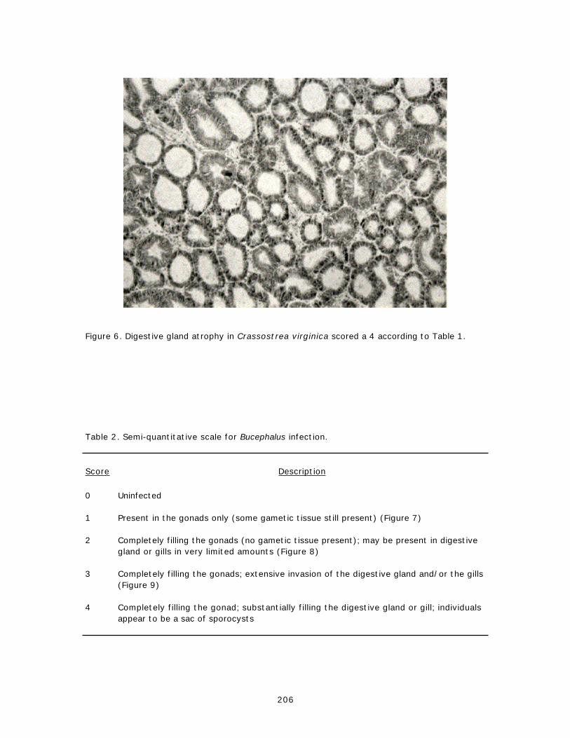
Figure 6. Digestive gland atrophy in Crassostrea virginica scored a 4 according to Table 1.

Table 2. Semi-quantitative scale for Bucephalus infection.

Score Description

0 Uninfected

1 Present in the gonads only (some gametic tissue still present) (Figure 7)

2 Completely filling the gonads (no gametic tissue present); may be present in digestivegland or gills in very limited amounts (Figure 8)

3 Completely filling the gonads; extensive invasion of the digestive gland and/or the gills(Figure 9)

4 Completely filling the gonad; substantially filling the digestive gland or gill; individualsappear to be a sac of sporocysts

206

Figure 7. Bucephalus infection in Mytilus edulis scored a 1 according to Table 2. Some gametictissue is still present.

Figure 8. Bucephalus infection in Mytilus edulis scored a 2 according to Table 2. No gametictissue is present.

207

Figure 9. Bucephalus infection in Mytilus edulis scored a 3 according to Table 2. No gametictissue is present. Bucephalus heavily infiltrating digestive gland.

Haplosporidium nelsoni [photograph: Ford and Tripp (1996), p. 614, Fig. 18] is a haplosporidianprotozoan responsible for MSX disease in oysters. The intensity of MSX infection is gradedaccording to a semi-quantitative scale (Table 3) reminiscent of the scale established forPerkinsus marinus. Because of the small size of H. nelsoni, oyster tissues may need to beexamined at a higher power than 10X, in some cases. Because MSX infection normally starts inthe gill epithelium, the gill tissue must be carefully examined to score early infectionsaccurately. In cases where the disease has become systemic, examination of the visceral massis necessary to score infection intensity. More details are provided in Ford (1985, 1986) andFord and Figueras (1988).

Several kinds of abnormal gonadal development have been observed, sometimes commonly, inmytilid mussels. Often, abnormal gonadal development is characterized by unusual developmentat the base of the follicles. The cells resemble that of a germinoma and are differentiated fromthat of normal development by being either enlarged, or appearing to have an enlarged nucleus.This type of abnormal development is more common in males than in females. In other cases,underdeveloped gonadal follicles were observed. Follicles were small and occupied a smallerportion of the mantle tissue. Ova were smaller and male follicles often had very few maturesperm. Sometimes follicles may be filled with anomalous ova or degenerating sperm, andgranulocytes, brown cells and cellular debris may clog the follicular lumens (Figure 10).Sometimes cells adhere to each other, forming accumulations and empty spaces amongdeveloping cells. Occasionally, fibrosis occurs, with proliferation of fibroblasts inside thefollicles and in the interfollicular connective tissue. Abnormal gonadal development is oftenassociated with degeneration of Leydig tissue around the follicles and hemocytic infiltrationinto the surrounding tissues (Figure 11).

208

Table 3. Semi-quantitative scale for Haplosporidium nelsoni infection [from Ford (1985, 1986)and Ford and Figueras (1988)].

Score Description

0 Uninfected

1 Epithelial only, rare to lightly infected, 1 - 100 parasites per field of gill tissue

2 Subepithelial, spreading into the visceral mass, lightly to moderately infected withclear subepithelial foci, normally 10 - >100 parasites per field but <5 parasites per1000X oil field

3 Subepithelial, more evenly distributed in visceral mass, lightly to moderately infectednormally 10 - >100 parasites per field but <5 parasites per 1000X oil field

4 Heavy systemic infection, averaging more than 5 parasites per oil field

Figure 10. Mytilus edulis follicle with abnormal gametic tissue (lower right).

209

Figure 11. Mytilus edulis follicle heavily infiltrated with hemocytes (right).

The approach used to score instances of abnormal gonadal development differs from that usedfor digestive gland atrophy in that the scale rates the spatial coverage of the condition (e.g.fraction of follicles affected), but not the degree of effect in each follicle (Table 4). Normally,the entire follicle is completely affected or not affected.

4. CONCLUSION

The described technique provides a quantitative or semi-quantitative method to determine theprevalence and intensity of parasites, pathologies, and diseases afflicting oysters, bluemussels and zebra mussels. The described method is a general approach for histopathologicalanalysis targeting a wide range of parasites and pathologies. Certain conditions will be betterassessed by other methods; Perkinsus marinus infection in oysters being a good example(Powell and Ellis, this volume). The described method emphasizes the quantification ofintensity. Prevalence rarely provides an adequate description of the population dynamics ofdisease and, in practice, often yields ambiguous results. Infection intensity quantitated bycounts or the use of a semi-quantitative scale consistently provides a more robust data set forstatistical analysis comparing the spatial and temporal distribution of parasites, pathologies,and diseases to contaminant body burden.

5. REFERENCES

Abbe, G. R., J. G. Sanders and G. F. Riedel (1994) Silver uptake by the oyster (Crassostreavirginica): effect of organisms size and storage sites. Estuarine Coastal Shelf Sci., 39:249-60.

210

Table 4. Semi-quantitative scale for abnormal gonadal development in mussels.

Score Description

0 Normal gonad

1 Less than half the follicles are affected

2 About half the follicles are affected

3 More than half the follicles are affected

4 All follicles affected

Ackerman, E., L. R. Elveback and J. P. Fox (1984) Simulation of infection disease epidemics.Charles C. Thomas, Springfield, 202 pp.

Anderson, R. S., L. M. Oliver and D. Jacobs (1992) Immunotoxicity of cadmium for the easternoyster (Crassostrea virginica [Gmelin, 1791]): effects of hemocyte chemiluminescence. J.Shellfish Res., 11: 31-5.

Axiak, V., J. J. George and M. N. Moore (1988) Petroleum hydrocarbons in the marine bivalveVenus verrucosa: accumulation and cellular responses. Mar. Biol. (Berl.), 97:225-30.

Barber, B. J. (1996) Gametogenesis of eastern oysters, Crassostrea virginica (Gmelin, 1791),and Pacific oysters, Crassostrea gigas (Thunberg, 1793) in disease-endemic lower ChesapeakeBay. J. Shellfish Res., 15:285-90.

Bielefeld, U. (1991) Histological observation of gonads and digestive gland in starvingDreissena polymorpha (Bivalvia). Malacologia, 33:31-42.

Bowmer, C. T., M. van der Meer and M. C. T. Scholten (1991) A histopathological analysis ofwild and transplanted Dreissena polymorpha from the Dutch sector of the River Maas. Comp.Biochem. Physiol. C, 100:225-9.

Cake Jr., E. W. (1977) Larval cestode parasites of edible mollusks of the northeastern Gulf ofMexico. Gulf. Res. Rpt., 6:1-8.

Cake Jr., E. W. and R. W. Menzel (1980) Infections of Tylocephalum metacestodes incommercial oysters and three predaceous gastropods of the eastern Gulf of Mexico. Proc. Natl.Shellfish. Assoc., 70:94-104.

Cheng, T. C. (1967) Marine molluscs as hosts for symbioses with a review of known parasitesof commercially important species. Adv. Mar. Biol., Vol. 5, Academic Press, London, 424 pp.

Cheng, T. C. (1988) In vivo effects of heavy metals on cellular defense mechanisms ofCrassostrea virginica: Total and differential cell counts. J. Invertebr. Pathol., 51:207-14.

211

Choi, K-S., D. H. Lewis, E. N. Powell and S. M. Ray (1993) Quantitative measurement ofreproductive output in the American oyster, Crassostrea virginica (Gmelin), using anenzyme-linked immunosorbent assay (ELISA). Aquacult. Fish. Management, 24:299-322.

Cunningham, P. A., and M. R. Tripp (1975) Accumulation, tissue distribution and elimination of203HgCl2 and CH3

203HgCl in the tissues of the American oyster Crassostrea virginica. Mar.Ecol., 31:321-34.

Davis, C. V., and B. J. Barber. (1994) Size-dependent mortality in hatchery reared populationsof oysters, Crassostrea virginica, Gmelin 1791, affected by juvenile oyster disease. J.Shellfish Res., 13:137-42.

Dungan, C. F., R. A. Elston and M. H. Schiewe (1989) Evidence for colonization and destructionof hinge ligaments in cultured juvenile Pacific oysters (Crassostrea gigas) by cytophaga-likebacteria. Appl. Environ. Microbiol., 55:1128-35.

Ellis, M. S., K-S. Choi, T. L. Wade, E. N. Powell, T. J. Jackson and D. H. Lewis (1993) Sourcesof local variation in polynuclear aromatic hydrocarbon and pesticide body burden in oysters(Crassostrea virginica) from Galveston Bay, Texas. Comp. Biochem. Physiol. C, 106:689-98.

Elston, R. A., A. S. Drum and S. K. Allen, Jr. (1990) Progressive development of circulatingpolyploid cells in Mytilus with hemic neoplasia. Dis. Aquat. Org., 8:51-9.

Farley, C. A. (1969) Probable neoplastic disease of the hematopoietic system in oysters,Crassostrea virginica and Crassostrea gigas. Natl. Cancer Inst. Monogr., 31:541-55.

Farley, C. A. (1976) Proliferative disorders in bivalves mollusks. Mar. Fish. Rev., 38:30-3.

Figueras, A. J., C. F. Jardon and J. R. Caldas. (1991) Diseases and parasites of mussels(Mytilus edulis, Linnaeus, 1758) from two sites on the east coast of the United States. J.Shellfish Res., 10:89-94.

Ford, S. E. (1985) Chronic infections of Haplosporidium nelsoni (MSX) in the oysterCrassostrea virginica. J. Invertebr. Pathol., 45:94-107.

Ford, S. E. (1986) Comparison of hemolymph proteins from resistant and susceptible oysters,Crassostrea virginica, exposed to the parasite Haplosporidium nelsoni (MSX). J. Invertebr.Pathol., 47:283-94.

Ford, S. E. (1988) Host-parasite interactions in eastern oysters selected for resistance toHaplosporidium nelsoni (MSX) disease: survival mechanisms against a natural pathogen. In:Disease processes in marine bivalve molluscs. W. S. Fisher (Ed.). Am. Fish. Soc. Spec. Publ.,18:206-24.

Ford, S. E., and A. J. Figueras (1988) Effects of sublethal infection by the parasiteHaplosporidium nelsoni (MSX) on gametogenesis, spawning, and sex ratios of oysters inDelaware Bay, USA. Dis. Aquat. Org., 4:121-33.

Ford, S. E., and M. R. Tripp (1996) Diseases and defense mechanisms. In: The eastern oysterCrassostrea virginica. V. S. Kennedy, R. I. E. Newell and A. F. Eble (Eds.), Maryland Sea GrantCollege, University of Maryland, College Park, MD. 581-660.

212

Gauthier, J. D., T. M. Soniat and J. S. Rogers (1990) A parasitological survey of oysters alongsalinity gradients in coastal Louisiana. J. World Aquaculture Soc., 21:105-15.

Gee, J. M., and J. T. Davey. (1986) Experimental studies on the infestation of Mytilus edulis(L.) by Mytilicola intestinalis Steuer (Copepoda, Cyclopoida). J. Cons. Int. Explor. Mer.,42:265-71.

Harshbarger, J. C., S. C. Chang and S. V. Otto (1977) Chlamydiae (with phages), mycoplasmas,and rickettsiae in Chesapeake Bay bivalves. Science, 196:666-8.

Harshbarger, J. C., S. V. Otto and S. C. Chang (1979) Proliferative disorders in Crassostreavirginica and Mya arenaria from the Chesapeake Bay and intranuclear virus-like inclusions inMya arenaria with germinomas from a Maine oil spill site. Haliotis, 8:243-8.

Hofmann, E. E., E. N. Powell, J. M. Klinck, and G. Saunders (1995) Modeling diseased oysterpopulations I. Modelling Perkinsus marinus infections in oysters. J. Shellfish Res., 14:121-51.

Hopkins, S. H. (1957) Our present knowledge of the oyster parasite "Bucephalus". Proc. Natl.Shellfish. Assoc., 47:58-61.

Johnson, L. L., C. M. Stehr, O. P. Olson, M. S. Myers, S. M. Pierce, B. B. McCain and U.Varanasi (1992) National benthic surveillance project: northeast coast. Fish histopathology andrelationships between lesions and chemical contaminants (1987-89). NOAA Tech. Memo.NMFS-NWFSC-4. NOAA/NMFS, Seattle, WA. 95 pp.

Kennicutt II, M. C. (ed.) (1995) Gulf of Mexico Offshore Operations Monitoring Experiment.Phase I: Sublethal responses to contaminant exposure. Final report. OCS Study MMS 95-0000.Dept. of the Interior, Minerals Management Service, Gulf of Mexico OCS Region, New Orleans,LA. 705 pp.

Kermack, W. O., and A. G. McKendrick (1991) Contributions to the mathematical theory ofepidemics. - I. Bull. Math. Biol., 53:33-55.

Laird, M. (1961) Microecological factors in oyster epizootics. Can. J. Zool., 39:449-85.

Landau, H., and P. S. Galtsoff (1951) Distribution of Nematopsis infection on the oyster groundsof the Chesapeake Bay and in other waters of the Atlantic and Gulf states. Tex. J. Sci.,3:115-30.

Landsberg, J. H. (1996) Neoplasia and biotoxins in bivalves: is there a connection? J. ShellfishRes., 15:203-30.

Lawler, I. F. and J. C. Aldrich (1987) Sublethal effects of bis(tri-N-butyltin)oxide onCrassostrea gigas spat. Mar. Pollut. Bull., 6:274-8.

Lee, M., G. T. Taylor, V. M. Bricelj, S. E. Ford and S. Zahn (1996) Evolution of Vibrio spp. andmicroplankton blooms as causative agents of juvenile oyster disease in Crassostrea virginica(Gmelin). J. Shellfish Res., 15:319-29.

213

Lee, R. F. (1993) Passage of xenobiotics and their metabolites from hepatopancreas into ovaryand oocytes of blue crabs, Callinectes sapidus: possible implications for vitellogenesis. Mar.Environ. Res., 35:181-7.

Little, J. W., S. H. Hopkins and J. G. Mackin (1969) The viability of an echinostomemetacercaria in the American oyster, Crassostrea virginica. J. Invertebr. Pathol., 13:455-6.

Marigómez, J. A., V. S. Sáez, M. P. Cajaraville and E. Angulo (1990) A planimetric study of themean epithelial thickness (MET) of the molluscan digestive gland over the tidal cycle and underenvironmental stress conditions. Helgol. Meeresunters., 44:81-94.

Mo, C. and B. Neilson (1993) Weight and salinity effects on zinc uptake and accumulation for theAmerican oyster (Crassostrea virginica Gmelin). Environ. Pollut., 82:191-6.

Murchelano, R. A., and S. A. MacLean (1990) Histopathology atlas of the registry of marinepathology. NOAA/NOS/National Ocean Pollution Program Office, Oxford, Maryland. 77 pp.

Peters, E. C. (1988) Recent investigations on the disseminated sarcomas of marine bivalvemolluscs. In: Disease processes in marine bivalve molluscs. W. S. Fisher (Ed.). Am. Fish. Soc.Spec. Publ., 18:74-92.

Powell, E. N., J. M. Klinck and E. E. Hofmann (1996) Modeling diseased oyster populations. II.Triggering mechanisms for Perkinsus marinus epizootics. J. Shellfish Res., 15:141-65.

Quick, J. A., and J. G. Mackin (1971) Oyster parasitism by Labyrinthomyxa marina in Florida.Fl. Dept. Nat. Resour. Mar. Res. Lab. Prof. Pap, 13:1-55.

Sindermann, C. J. (1970) Principal diseases of marine fish and shellfish. Academic Press, Inc.,New York, NY. 369 pp.

Sparks, A. K. (1985) Synopsis of invertebrate pathology exclusive of insects. Elsevier SciencePublishers, Amsterdam, Netherlands. 423 pp.

Sprague, V., and P. E. Orr (1952) Studies on Nematopsis. III. N. ostrearum and N. prytherchiwith special reference to host-parasite relation. Natl. Shellfish. Assoc. Conv. Add., p. 26-43.

Sprung, M. (1991) Costs of reproduction: a study on metabolic requirements of the gonads andfecundity of the bivalve Dreissena polymorpha. Malacologia, 33:63-70.

Warburton, F. E. (1958) Control of the boring sponge on oyster beds. Fish. Res. Board Can.Prog. Rpt. Atl. Coast Stns., 69:7-11.

Weis, P., J. S. Weis, J. Couch, C. Daniels and T. Chen (1995) Pathological and genotoxicologicalobservations in oysters (Crassostrea virginica) living on chromated copper arsenate(CCA)-treated wood. Mar. Environ. Res., 39:275-8.

White, M. E., C. L. Kitting and E. N. Powell (1985) Aspects of reproduction, larval developmentand morphometrics in the pyramidellid Boonea (=0dostomia) impressa (Gastropoda:Opisthobranchia). Veliger, 28:37-51.

214

White, M. E., E. N. Powell, E. A. Wilson and S. M. Ray (1989) The spatial distribution ofPerkinsus marinus, a protozoan parasite, in relation to its oyster host (Crassostrea virginica)and an ectoparasitic gastropod (Boonea impressa). J. Mar. Biol. Assoc. UK, 69:703-17.

Winstead, J. T. (1995) Digestive tubule atrophy in Eastern oysters, Crassostrea virginica(Gmelin, 1791), exposed to salinity and starvation stress. J. Shellfish Res., 14:105-11.

Winstead, J. T., and J. A. Couch (1981) Proctoeces sp. (Trematoda: Digenea) in the Americanoyster, Crassostrea virginica. Trans. Am. Micros. Soc., 100:296-305.

Winstead, J. T., and J. A. Couch (1988) Enhancement of protozoan pathogen Perkinsus marinusinfections in American oysters Crassostrea virginica exposed to the chemical carcinogenn-nitrosodiethylamine (DENA). Dis. Aquat. Org., 5:205-13.

Wolf, P. H., J. T. Winstead and J. A. Couch (1987) Proctoeces sp. (Trematoda: Digenea) inAustralian oysters, Saccostrea commercialis and Crassostrea amasa. Trans. Am. Micros. Soc.,106:379-80.

Yoo, M. S., and T. Kajihara (1985) Effect of the pea crab (Pinnotheres pholadis) on thereproductive capacity of the blue mussel (Mytilus edulis galloprovincialis). Bull. Korean Fish.Soc., 18:581-5.

Zaroogian, G., and P. Yevich (1993) Effect of selected inhibitors on cadmium, nickel, andbenzo[a]pyrene uptake into brown cells of Mercenaria mercenaria. Mar. Environ. Res.,35:41-5.

215

Gonadal Analysis

M. S. Ellis, R. D. Barber, R. E. Hillman,* and E. N. PowellHaskin Shellfish Research Laboratory


ABSTRACT

This document describes the procedures for determining the reproductive stage ofoysters, mussels, and zebra mussels collected for NOAA's National Status and TrendsMussel Watch Program. Procedures are documented for preparation ofparaffin-embedded tissues sectioned at a 5-µm thickness and stained using apentachrome staining procedure.

1. INTRODUCTION

Assessment of the physiological state of bivalve populations requires an analysis of the stateof gonadal development. Determination of reproductive stage was included as part of the MusselWatch Project to give an indication of the amount of gametic material in the bivalves' tissues atthe time of chemical analysis. Certain contaminants are preferentially concentrated in gonadaltissue (Ellis et al., 1993; Lee, 1993; Abbe et al., 1994). Others are concentrated innon-gonadal tissue (Mo and Neilson, 1993; Cunningham and Tripp 1975). Because gameticmaterial can account for 20% to 50% of body weight in target species of oysters and mussels(Sprung, 1992; Choi et al., 1993), the relative proportion of gonadal to somatic tissue and thetiming of spawns (an important depuration route for some contaminants) can significantlyimpact the body burden of contaminants.

The original intent of the determinations of reproductive stage was to assure that sampling wasconducted at the same stage of the reproductive cycle so that analysis of neither the lipophilicorganic contaminants nor the trace element contaminants were influenced by reproductivestate. Unfortunately, the time required for sampling and the wide latitudinal range encompassedby the sites did not permit consistent recovery of individuals in a similar stage of reproductivedevelopment at all sites. For example, typically, oysters are undifferentiated in the winter.Gonads begin to develop in early spring and spawning occurs during late spring through earlyfall. Most Gulf Coast oysters spawn at least twice during this time period. Single spawns tendto occur in the shorter summers of the mid-Atlantic region. The timing of the last spawn varieswith latitude and with yearly variations in climate (e.g. Wilson et al., 1990, 1992). Certainsites, particularly southeast Atlantic and southern Gulf sites, routinely yield oysters inreproductive development or ready to spawn in mid-winter during the period when MusselWatch sampling occurs at these sites. Mid-Atlantic sites typically were characterized byindividuals in an undifferentiated state, that thus contained significantly less lipid-rich gametictissue and that had been accumulating contaminants for a much longer time since their mostrecent spawn. Mytilids and zebra mussels had the same assortment of problems relating tolatitude and interannual changes in climate (Newell, 1989; Seed and Suchanek, 1992;Borcherding, 1991). Thus, analysis of reproductive stage proved important in identifyingdifferences in tissue composition which might affect between site and interannual comparisons

* Battelle Ocean Sciences, Environmental Assessment Division, Duxbury, MA 02332.

216

of contaminant data. Wilson et al. (1990, 1992) discuss the influence of climate onreproductive stage and contaminant body burden in the Mussel Watch Program in more detail.

Oyster gonadal tissue is distributed around the body mass and cannot be easily excised andweighed (Morales-Alamo and Mann, 1989). In contrast to oysters, in mussels the gonadalfollicles develop primarily within the mantle. Zebra mussel gonads develop within the body,around the periphery of the viscera. In none of these cases can the gonad be easily excised andweighed. Consequently, virtually all assays of reproductive stage use histological methods torecognize the changes in the germinal epithelium and germinal products that identify stages ingonadal development. The histological approach uses a semiquantitative numerical assignment torank reproductive stage. Quantitative measures, such as a measure of egg protein content (Choiand Powell, 1993), remain expensive and time consuming, and do not permit a concomitanthistopathological analysis. Therefore, a histological examination is still the single method ofchoice, when only one method can be used.

For oysters and mytilid mussels, a dorsal-ventral slice of tissue is taken and fixed inDavidson's fixative. Zebra mussels are decalcified and embedded whole. Tissue samples areembedded in paraffin, sectioned, and stained using a pentachrome staining protocol. Stainedsections are examined under a compound microscope, and sex and the state of gonadaldevelopment determined. Fixation follows the method described in Preece (1972). The stainingprocedure is an adaptation by one of us (Barber) of Masson's (1928) trichrome procedure.Reproductive stage in oysters is determined using a semiquantitative scale adapted from Fordand Figueras (1988). The scale developed by Seed (1975, 1976) for determining gonad index inmussels was adopted for mussels and zebra mussels.

2. EQUIPMENT, REAGENTS AND SOLUTIONS

2.1. Equipment

Stainless steel molds, various sizes. Fisher Scientific, Pittsburgh, PA.Disposable microtome blades, 12-634-11. Fisher Scientific, Pittsburgh, PA..Cover slips - square no. 1, 22 mm x 22 mm, 12-531-A. Fisher Scientific, Pittsburgh, PA.Disposable cassettes - HistoPrep tissue capsules, 15-182-218. Fisher Scientific, Pittsburgh,

PA.Paraffin embedding center, 12-653-68. Fisher Scientific, Pittsburgh, PA.Embedding rings - HistoPrep embedding rings, 12-652-1OB. Fisher Scientific, Pittsburgh, PA.Frosted microslides, 12-552. Fisher Scientific, Pittsburgh, PA.Microscope, compound, Zeiss, 12-070-20. Fisher Scientific, Pittsburgh, PA.Microtome, Leica Histocut 820 Rotary microtome, 12-603. Fisher Scientific, Pittsburgh, PA.Microtome knife sharpener, automatic, Leica 903, 12-643-40. Fisher Scientific, Pittsburgh,

PA.Drying oven, 13-254-1. Fisher Scientific, Pittsburgh, PA.Paraffin pitcher, electric, Lepshaw 220, M7395. Baxter Scientific, McGaw Park, IL.Rotary tissue processor, Tissue-Tek, M7286-1. Baxter Scientific, McGaw Park, IL.Slide warmer, 12-594. Fisher Scientific, Pittsburgh, PA.Staining dishes, 08-813A. Fisher Scientific, Pittsburgh, PA.Vacuum oven, 13-264A. Baxter Scientific, McGaw Park, IL.Water bath - Fisher Tissue PrepModel 134 Flotation Bath, 15-464. Fisher Scientific,

Pittsburgh, PA.

217

2.2. Reagents

Acid fuchsin, certified stain (C20H17N3Na2O9S3) [3244-88-0], A3908. Sigma Chemical Co.,St.Louis, MO.

Ammonium hydroxide (NH4OH) [1336-21-6], A6899. Sigma Chemical Co., St. Louis, MO.Aniline blue powder, certified stain [28631-66-5], A697-25. Fisher Scientific, Pittsburgh,

PA.Chromotrope powder 2R, (C16H10N2Na2O8S2) [4197-07-3], C3143. Sigma Chemical Co., St.

Louis, MO.Ethanol (C2H6O) [64-17-5], R8382. Sigma Chemical Co., St. Louis, MO.Fast green FCF, certified stain (C37H34N2O10S3Na2) [2353-45-9], F7252. Sigma Chemical Co.,

St. Louis, MO.Ferric ammonium sulfate [NH4Fe(SO4)2 . 12H2O] [7783-83-7], F1018. Sigma Chemical Co., St.

Louis, MO.Formaldehyde, 37% solution (CH2O) [50-00-0], F1635. Sigma Chemical Co., St. Louis, MO.Glacial acetic acid (C2H402) [64-19-7], A0808. Sigma Chemical Co., St. Louis, MO.Glycerin (C3H803) [56-81-5], G7893. Sigma Chemical Co., St. Louis, MO.Hematoxylin powder, certified stain (C16H1406) [517-28-2], H3136. Sigma Chemical Co., St.

Louis, MO.Hydrochloric acid, 12 N, (HCI) [7647-01-0], H7020. Sigma Chemical Co., St. Louis, MO.Orange G powder, certified stain (C16H10N2O7S2Na2) [1936-15-8], 07252. Sigma Chemical

Co., St. Louis, MO.Paraffin - Paraplast tissue embedding media (melting pt. 56 °C), 12-464-11, Fisher Scientific,

Pittsburgh, PA.Permount mounting media, SP15-500. Fisher Scientific, Pittsburgh, PA.Phosphomolybdic acid (24MoO3 . P2O5 . H2O) [51429-74-4], P7390. Sigma Chemical Co., St.

Louis, MO.Phosphotungstic acid (12WO3 . H3PO4 . H2O) [12501-23-4], P4006. Sigma Chemical Co., St.

Louis, MO.Sodium chloride (NaCI) [7647-14-5], S9625. Sigma Chemical Co., St. Louis, MO.Sulfuric acid (H2SO4) [7664-93-9], S1526. Sigma Chemical Co., St. Louis, MO.Tissue Clear II, SH2-4. Fisher Scientific, Pittsburgh, PA.Tissue Dry, SH5-20. Fisher Scientific, Pittsburgh, PA.Xylenes, histological grade (C8H10), X35-4. Sigma Chemical Co., St. Louis, MO.

2.3. Solutions

Ferric alum mordant: 25 g ferric ammonium sulfate dissolved in 500 mL distilled water.

Basic ethanol: 26 mL ammonium hydroxide in a solution of 3370 mL 95% ethanol and 630 mLdistilled water.

Phosphomolybdic acid solution: 5 g phosphomolybdic acid dissolved in 495 mL distilled water.

1% acetic acid: 20 mL glacial acetic acid in 1980 mL distilled water.

1% acid acetone: 20 mL acetone in 1980 mL distilled water

Groat/Weigert hematoxylin working solution: 245 mL distilled water, 5 mL sulfuric acid, 5 gferric ammonium sulfate, 245 mL 95% ethanol, and 2.5 g hematoxylin powder.

218

Acid fuchsin working solution: 2.5 g acid fuchsin powder dissolved in 495 mL distilled water, towhich is added 5 mL glacial acetic acid.

Phosphotungstic acid solution: 10 g phosphotungstic acid dissolved in 490 mL distilled water.

Orange G - stock: 4 g orange G powder dissolved in 495 mL distilled water to which was added5 mL glacial acetic acid.

Chromotrope 2R - stock: 3 g chromotrope powder dissolved in 495 mL distilled water to whichwas added 5 mL glacial acetic acid.

Orange G/Chromotrope working stock: 400 mL orange G solution and 100 mL chromotropesolution.

Fast green - stock: 8 g fast green FCF dissolved in 495 mL distilled water to which was added 5mL glacial acetic acid.

Aniline blue - stock: 6 g aniline blue powder in 495 mL distilled water.

Fast green/Aniline blue working solution: 150 mL fast green solution and 350 mL aniline bluesolution.

Davidson's fixative stock solution: 1 part glycerin, 2 parts 37 - 40% formaldehyde, 3 parts95% ethanol, and 3 parts isotonic sodium chloride (usually 20 - 30o/oo). The solution wasstored at 4 °C.

Davidson's fixative working solution: Just before use, 1 part of glacial acetic acid was mixedwith 9 parts of the stock solution.

3. SAMPLE COLLECTION AND FIXATION

3.1. Sampling

From 1986 to 1994, the same oysters were used for organic contaminant analysis and gonadalanalysis at all Gulf coast sites (Powell et al., 1993). The use of the same animals for gonadalanalysis and for the analysis of contaminant body burden potentially biases the latter analysesbecause digestive gland tissue and gonadal tissue, which contribute a disproportionate portionof the tissue taken for histological analysis, may contain a higher than average body burden ofcertain contaminants. Sericano et al. (1993) showed that this source of error resulted in anunderestimation of true body burden by no more than 10% under most conditions for the largeoysters used in the Mussel Watch Program, if the slice of tissue removed was limited to a 3 to5 mm section. The potential error would be much larger for the smaller mytilids and zebramussels. In order to avoid this error, separate samples were obtained for the gonadal analysisportion of the Mussel Watch project for these species (and East coast oysters) in all years,and, beginning in 1995, the same protocol was adopted for the Gulf coast oysters. Thus, thepresent sampling method requires the assumption in all cases that individuals collected from acommon collection area will have experienced similar chemical loading and therefore avoid theerror introduced by subsampling the tissue to be analyzed for contaminants.

219

1 2 3 4 50cm

Gill

Mouth

Labial palps

Shell

Tissue taken forgonadal analysis

Anus

Digestive gland

Figure 1. Oyster tissue used for quantifying reproductive stage (adapted from Galtsoff,1964).

3.2. Tissue preparation

3.2.1. Oyster tissue preparation

Each oyster was opened with an oyster knife by cutting the adductor muscle at its connectionwith the upper shell. A 3- to 5-mm thick cross-section of tissue was removed from the oysterusing a scalpel or scissors (Figure 1). The determination of reproductive stage is based on ahistological evaluation of the maturation stage of oyster gonads, which are located around thevisceral mass. The tissue section is obtained such that the dorsal-ventral aspect passesthrough the digestive gland and gill tissue just posterior to the palps. This aspect providesexample sections of most oyster tissues for histopathological analysis (Ellis et al., thisvolume), while also providing a representative cross-section of oyster gonad.

Each section was immediately placed in a tissue cassette and the cassette placed in a jar filledwith Davidson's fixative for 48 hr. Bouin's fixative is an adequate alternative in mostapplications. After 48 hr, the fixative was decanted, 50% ethanol added and the tissues

220

allowed to stand for 2 hr, during which time the vials are occasionally shaken. After 2 hr, the50% ethanol solution was replaced with 70% ethanol, and the vials shaken every few hours.After 24 hr, the 70% ethanol was replaced with fresh 70% ethanol for storage untilprocessing.

3.2.2. Mussel tissue preparation

Determination of reproductive stage for mussels was based on a histological evaluation of thematuration stage of mussel gonads, most of which are located in the mantle (Newell, 1989).Ordinary means of removal of mussels from their shells usually resulted in severe damage tothe mantle tissue lying next to the shell. Therefore, it was easier to preserve the mussels intheir shells. Once preserved, the tissue hardened and become easier to dissect.

The tip of a sharp knife was carefully inserted between the shells at the ventral lip and rundorsally between the shells until the adductor muscle cut so that the shells remain in an openposition. Care was taken to cut no further than the adductor muscle to avoid cutting into thedigestive gland immediately below the adductor muscle. The mussels were then placed in awide-mouth jar filled with Davidson's fixative. Because the entire animal was being preserved,the specimens were usually left in fixative for at least a week to ensure preservation of alltissues. After this time, the fixative was decanted, 50% ethanol added, and the tissue allowedto stand for 48 hr, during which time the jar was shaken occasionally. The solution was thenpoured off, 70% ethanol added and the mixture allowed to stand for 72 hr, after which the 70%ethanol can be replaced with fresh 70% ethanol for storage until processing.

To excise the mussel meat from its shell, a scalpel was carefully run between the mantle andthe lip of the shell, detaching the mantle from the shell. This was done around thecircumference of one of the shells and the scalpel then used to carefully separate the meat fromthe shell. This procedure was repeated for the other shell. A 3 - 5 mm thick cross-section,obtained such that the dorsal-ventral aspect passes through the digestive gland at an angleacross the body slightly toward the forward edge, was then removed using a scalpel orscissors. Each section was placed in a tissue cassette and processed immediately afterdissection.

If the mantle tissue was damaged during the shell-opening procedure, the specimen wasdiscarded because the wound could result in the loss of gametic material, and lead to anerroneous evaluation. Some damage to the gills and viscera was acceptable, but care should betaken to minimize that damage, so the tissues may be used for histopathological evaluation(Ellis et al., this volume) as well as determination of reproductive stage.

3.2.3. Zebra mussel preparation

Most of the gonad of a zebra mussel was concentrated within the visceral mass (Borcherding,1990). Due to their small size however, dissection of living tissue without destroying thegonads is difficult. Therefore, zebra mussels were preserved whole, in their shells. Theanimals were placed whole, without bothering to cut the adductor muscle, into a jar withDavidson's fixative and left in fixative for one week to allow adequate time for tissue fixation.After this time, 20 to 30 mL of acetic acid was added to enhance decalcification of the shell.The shell was properly decalcified when examination by hand showed that the shell is no longerhard.

After decalcification was complete, the Davidson's was replaced with ethanol according to theprocedure followed for mussels. Once the zebra mussels were placed in the final 70% ethanolsolution, they were ready for embedding. Prior to embedding, a small tear was made in asection of the mantle away from the visceral mass to prevent air bubbles from forming within

221

the body cavity which limits proper infiltration of the paraffin. Byssal threads must also be cutaway from the byssal gland to prevent problems when sectioning the tissue.

4. SLIDE PREPARATION

4.1. Tissue embedding

Individual tissue samples were prepared for embedding in paraffin using an establisheddehydration protocol (Table 1). The solutions used for dehydration, clearing, and infiltrationwere changed frequently to maintain solution purity.

The tissue embedding sequence used an automated tissue processor which automaticallyprocesses tissue through the dehydration-clearing series and into paraffin. Embedding can alsobe done manually by moving the tissues through the sequence. The paraffin was melted in anoven set at no more than 2 °C above the melting temperature and kept at temperatures nohigher than 2 °C above melting during the infiltration process. Newly-melted paraffin shouldalways be used in the final infiltration and embedding steps.

After the tissues were infiltrated with paraffin (Table 1), they were transferred to a paraffinpot and placed under a vacuum for 30 min. The vacuum oven was set to maintain the paraffin atthe same carefully-controlled temperature. The tissues were then transferred to stainlesssteel molds filled with newly-melted paraffin. Oysters and mussels were orientedcross-sectional face down for sectioning, and a plastic mold embedding ring placed on top.Unlike the mytilids and the oysters, zebra mussels were embedded whole. Zebra mussels wereplaced on their side and, when the paraffin was added, care was taken to ensure that no airbubbles formed within the body cavity. The plastic backing was filled with paraffin and the moldmoved to a cold plate. As the tissue/paraffin cooled and hardened, the paraffin shrinks. Caremust be taken to use sufficient paraffin to cover the tissue after it cools and hardens.Occasionally, more paraffin must be added. The mold was left on the cold plate until thetissue-paraffin block was removed. The tissue-paraffin block was then placed in a freezer overnight before sectioning. When sectioning a number of blocks, the remaining blocks were placedin a tray of ice to keep them cold until sectioned.

Table 1. Tissue embedding sequence*.

Dehydration ClearingTissue Dry 60 min Tissue Clear 60 minTissue Dry 120 min Tissue Clear 120 minTissue Dry 120 min Tissue Clear 120 minTissue Dry 120 minTissue Dry 120 min InfiltrationTissue Dry 120 min paraffin 120 minTissue Dry 60 min paraffin 120 min

paraffin in vacuum oven 30 min

* In cases where the sequential solutions are the same, each transfer is a transfer to a fresh solution.

222

4.2. Tissue sectioning

The paraffin blocks were first cut at 20 µm to expose an entire tissue cross-section, and thensliced at 5 µm using an AO microtome. Tissue sections may be cut singly, or into contiguoussections. The tissue sections were placed on the surface of a water bath maintained at 45-50°C and allowed to expand. Once the sections expanded to full size, a microscope slide was heldat a 45° angle and slid under one or more of the tissue sections and the sections lifted out of thewater onto the slide. The sections were positioned on the slide in the orientation in which theywill be stained and read. The slide was then placed on a slide warmer until dry or allowed to airdry until it could be placed in a slide rack. The slide rack was placed in a drying oven overnightat 40 °C. After drying overnight, the slides were ready to stain.

4.3. Tissue staining

The staining procedure was Barber's adaptation of the trichrome stain of Masson (1928) asmodified by Gurr (1956). Barber's modifications include the addition of aniline blue to the fastgreen working solution, substitution of chromotrope 2A/orange G for Ponceau de Xylidene, andthe addition of phosphotungstic acid prior to the orange G/chromotrope stain; the procedure isnow a pentachrome technique. The addition of these stains yields better differentiation of tissuetypes and mucins. Times required for each step are flexible in both the staining proceduresdiscussed here and in the previous embedding protocol. Different tissue types may requiredifferent times. All tissue baths, especially xylene and ethanol ones, should be changedfrequently. Slides should not be allowed to dry during transfers. Solutions to commonembedding, sectioning, and staining problems are discussed in Preece (1972) and most othermanuals of histological technique.

Sections were deparaffinized and hydrated using a xylene-ethanol series (Table 2). Followinghydration, slides were stained in the pentachrome series, dehydrated in a series of acetic aciddips followed by acetone, cleared in xylene and mounted in Permount (Table 2).

5. ANALYSIS

Each slide was examined microscopically to determine sex and stage of gonadal development. Ahistopathological examination can also be made at this time, if desired (see Ellis et al., thisvolume). Careful examination of early developmental stages may be needed to positivelydistinguish males or females in early stages of development from individuals as yetundifferentiated. Occasional hermaphrodites will also be found (all target species normally haveseparate sexes). The stage in the gametogenic cycle was assigned based on the maturity of thefollicles and gametes and a numerical value assigned as described in Tables 3 and 4.

For mytilids and zebra mussels, a mean Gonadal Index can be determined from the sum of theindividual stage numbers. The index can vary from zero, if the entire population was spent orresting, to five, if the population was fully ripe.

Cases of renewed gonadal development following spawning (stage 7) were common in oysters,particularly along the Gulf of Mexico coast. These animals typically have a few remaininglarge, mature ova and many developing ova that would normally be found in stages 3 or 4.Accordingly, for oysters, further data reduction can better be achieved by comparing thenumber of individuals with substantial gonadal development with those having little gonadalvolume using an egg/eggless ratio, calculated as

= the number of individuals at stages 3, 4, 5, 6 and 7

the number of individuals at stages 1, 2 and 8

223

Table 2. Tissue staining sequence.

Deparaffinization Phosphotungstic acid 2 minxylene 5 min Orange G/Chromotrope stain 1.5 minxylene 5 min Running tap water* 5 minxylene 5 min Phosphomolybdic acid 2 min100% ethanol 3 min Fast Green/Aniline Blue stain 3 min100% ethanol 2 min

DehydrationHydration 1% acetic acid 20-25 dips

95% ethanol 2 min 1% acetic acid 20-25 dips10% ethanol 2 min 1% acetic acid 20-25 dipsdistilled water 2 min 1% acid acetone 20-25 dips

1% acid acetone 20-25 dipsStaining series 1% acid acetone 20-25 dips

Ferric Alum Mordant 6 minGroat/Weigert Hematoxylin 30-45 min ClearingRunning tap water 3 min xylene 5 minBasic ethanol 15 sec xylene 5 minRunning tap water 2 minAcid Fuchsin stain 1.5 min MountingRunning tap water* 5 min Mounting in Permount 24 hr to dry

* At these steps, no stain should remain between the slides and holding grooves in the slide rack

Table 3. Oyster development stages.

Developmental Stage Value Description

Sexually undifferentiated 1 Little or no gonadal tissue visibleEarly development 2 Follicles beginning to expandMid-development 3 Follicles expanded and beginning to coalesce; no mature

gametes presentLate development 4 Follicles greatly expanded, and coalesced, but

considerable connective tissue remaining; somemature gametes present

Fully developed 5 Most gametes mature; little connective tissueremaining

Spawning 6 Gametes visible in gonoductsSpawned 7 Reduced number of gametes; some mature gametes

still remaining; evidence of renewed reproductiveactivity

Spawned 8 Few or no gametes visible; gonadal tissue atrophying

224

Table 4. Mussel and zebra mussel development stages.

Reproductive stage Description

Resting/spent gonadStage 0 Inactive or undifferentiated

Developing gonadStage 1 Gametogenesis has begun; no ripe gametes visibleStage 2 Ripe gametes present; gonad developed to about one-third of its final sizeStage 3 Gonad increased in mass to about half the fully ripe condition; each follicle

contains, in area, about equal proportions of ripe and developing gametesStage 4 Gametogenesis still progressing, follicles contain mainly ripe gametes

Ripe gonadStage 5 Gonad fully ripe, early stages of gametogenesis rare; follicles distended

with ripe gametes; ova compacted into polygonal configurations; spermwith visible tails

Spawning gonadStage 4 Active emission has begun; sperm density reduced; ova rounded off as

pressure within follicles is reducedStage 3 Gonad about half emptyStage 2 Gonadal area reduced; follicles about one-third full of ripe gametesStage 1 Only residual gametes remain; some may be undergoing cytolysis

6. CONCLUSIONS

The procedures describe provide a semiquantitative ranking of reproductive stage but noquantification of the amount of gametic tissue present. The strengths of this approach are thatit provides an assessment of sexual stage in the gametogenic cycle, and, if desired, allows fora concomitant histopathological analysis, with a single sample preparation protocol. Theprocedure cannot be performed on pooled samples, thus necessitating individual analysis of afraction of the samples pooled for other purposes or analysis of separate individuals. Thus, adirect correspondence between, for example, hydrocarbon body burden and stage in thegametogenic cycle may be difficult, because subsampling of individual animals will result in acertain degree of bias in the measurement of contaminant body burden, normally around 10% inadult oysters (Sericano et al., 1993) and more for smaller species. This bias, therefore, willbe size-, contaminant-, and time of year dependent.

If a quantitative gonadal/somatic index is desired, the technique of Choi and Powell (1993)should be used. The latter technique measures the concentration of egg protein present,however, it is not compatible with a concomitant histopathological analysis in that the standardhistological preparation for assessing reproductive stage is not used in the quantitativeanalysis and tissue subsampling for histology cannot be done on the same individuals to beanalyzed quantitatively for gonadal-somatic index. Choi et al. (1993) have further discussedthe relative value of various approaches to gonadal evaluation. Overall, these authors foundthat the same general trends could be identified using either the semiquantitative orquantitative technique in most species, because normally an increase in gonadal volume occurs

225

more or less simultaneously with advancement in reproductive stage and because gametematuration occurs more or less evenly throughout the entire gonad.

7. REFERENCES

Abbe, G. R., J. G. Sanders and G. F. Riedel (1994) Silver uptake by the oyster (Crassostreavirginica): effect of organisms size and storage sites. Estuarine Coastal Shelf Sci., 39:249-60.

Borcherding, J. (1990) Die Reproduktionsleistungen der Wandermuschel Dreissena polymorpha.Ph.D. Dissertation, Universität zu Köln, Germany. 168 pp.

Borcherding, J. (1991) The annual reproductive cycle of the freshwater mussel Dreissenapolymorpha Pallas in lakes. Oecologia (Berl.), 87:208-18

Choi, K-S., D. H. Lewis, E. N. Powell and S. M. Ray (1993) Quantitative measurement ofreproductive output in the American oyster, Crassostrea virginica (Gmelin), using anenzyme-linked immunosorbent assay (ELISA). Aquacult. Fish. Management, 24:299-322.

Choi, K-S., and E. N. Powell (1993) Development of and immunological probe for quantificationof oyster gonad. In: Sampling and analytical methods of the National Status and Trends ProgramNational Benthic Surveillance and Mussel Watch Projects 1984-1992. Vol. II Comprehensivedescriptions of complementary measurements. NOAA Tech. Mem. NOS ORCA 71.NOAA/NOS/ORCA, Silver Spring, MD. 85-102.

Cunningham, P. A., and M. R. Tripp (1975) Accumulation, tissue distribution and elimination of203HgCl2 and CH3

203HgCl in the tissues of the American oyster Crassostrea virginica. Mar.Ecol., 31:321-34.

Ellis, M. S., K-S. Choi, T. L. Wade, E. N. Powell, T. J. Jackson and D. H. Lewis (1993) Sourcesof local variation in polynuclear aromatic hydrocarbon and pesticide body burden in oysters(Crassostrea virginica) from Galveston Bay, Texas. Comp. Biochem. Physiol. C, 106:689-98.

Ford, S. E., and A. J. Figueras (1988) Effects of sublethal infection by the parasiteHaplosporidium nelsoni (MSX) on gametogenesis, spawning, and sex ratios of oysters inDelaware Bay, USA. Dis. Aquat. Org., 4:121-33.

Galtsoff, P. S. (1964) The American oyster Crassostrea virginica Gmelin. U.S. Fish Wildl.Serv. Fish. Bull. 64. U.S. Government Printing Office, Washington, D.C. 480 pp.

Gurr, E. (1956) A Practical Manual of Medical and Biological Staining Techniques. Interscience,New York. 320 pp.

Lee, R. F. (1993) Passage of xenobiotics and their metabolites from hepatopancreas into ovaryand oocytes of blue crabs, Callinectes sapidus: possible implications for vitellogenesis. Mar.Environ. Res., 35:181-7.

Masson, P. (1928) Carcinoids (argentaffin cell tumors) and nerve hyperplasia of theappendicular mucosa. Am. J. Pathol., 4:181-211.

226

Mo, C., and B. Neilson (1993) Weight and salinity effects on zinc uptake and accumulation forthe American oyster (Crassostrea virginica Gmelin). Environ. Pollut., 82:191-6.

Morales-Alamo, R., and R. Mann (1989) Anatomical features in histological sections ofCrassostrea virginica (Gmelin, 1791) as an aid in measurements of gonad area forreproductive assessment. J. Shellfish Res., 8:71-82.

Newell, R. I. E. (1989) Species profiles: life histories and environmental requirements ofcoastal fishes and invertebrates (North and Mid-Atlantic) - blue mussel. U.S. Fish. Wildl. Serv.Biol. Rep. 82(11.102). U.S. Army Corps of Engineers, TR E1-82-4. 25 pp.

Powell, E. N., E. A. Wilson-Ormond and K-S. Choi (1993) Gonadal analysis - Crassostreavirginica. In: Sampling and analytical methods of the National Status and Trends ProgramNational Benthic Surveillance and Mussel Watch Projects 1984-1992. Vol. II Comprehensivedescriptions of complementary measurements. NOAA Tech. Mem. NOS ORCA 71.NOAA/NOS/ORCA, Silver Spring, MD. 55-62.

Preece, A. (1972) A Manual for Histologic Technicians. Little, Brown, and Company, Boston.428 pp.

Seed, R. (1975) Reproduction in Mytilus (Mollusca: Bivalvia) in European waters. Pubblicazionidella Stazione Zoologica di Napoli (Milan), 39(Suppl. 1):317-334.

Seed, R. (1976) Ecology. In: Marine Mussels: Their Ecology and Physiology. B. L. Bayne (ed.).Cambridge University Press, New York, NY. 13-66.

Seed, R., and T. H. Suchanek (1992) Population and community ecology of Mytilus. In: TheMussel Mytilus: Ecology, Physiology, Genetics and Culture. E. Gosling (Ed.). Developments inAquaculture and Fisheries Science, 25:87-169.

Sericano, J. L., T. L. Wade, E. N. Powell, and J. M. Brooks (1993) Concurrent chemical andhistological analyses: are they compatible? Chem. Ecol., 8:41-7.

Sprung, M. (1991) Costs of reproduction: a study on metabolic requirements of the gonads andfecundity of the bivalve Dreissena polymorpha. Malacologia, 33:63-70.

Wilson, E. A., E. N. Powell, M. A. Craig, T. L. Wade, and J. M. Brooks (1990) The distribution ofPerkinsus marinus in Gulf coast oysters: its relationship with temperature, reproduction, andpollutant body burden. Int. Rev. Gesamten Hydrobiol., 75:533-50.

Wilson, E. A., E. N. Powell, T. L. Wade, R. J. Taylor, B. J. Presley and J. M. Brooks (1992)Spatial and temporal distributions of contaminant body burden and disease in Gulf of Mexicooyster populations: the role of local and large-scale climatic controls. Helgol. Meeresunters.,46:201-35.

227

Perkinsus marinus Assay

E. N. Powell and M. S. EllisHaskin Shellfish Research Laboratory


USA

ABSTRACT

This document describes the procedures followed for the assay of Perkinsus marinusprevalence and infection intensity in oyster specimens collected on the East and GulfCoasts of the US and in Puerto Rico by Rutgers University for the National Oceanic andAtmospheric Administration's National Status and Trends Program Mussel WatchProject.

1. INTRODUCTION

The determination of the health of oyster populations requires an analysis of Perkinsusmarinus prevalence and infection intensity. P. marinus is the most serious disease-producingpathogen of East and Gulf coast oysters. This standard operating procedure is the accepted bestmethod for quantitating the presence of this parasite when an approximate or exactquantification of disease intensity is required. A tissue homogenate or a section of mantletissue is incubated in thioglycollate medium for 14 days according to the method of Ray (1966).A semiquantitative (Craig et al., 1989) or quantitative (Choi et al., 1989) assessment ofhypnospore number is then made microscopically.


2.1. Reagents

2.1.1. Chemicals

Chloramphenicol (chloromycetin), (C11H12C12N2O5) [56-75-7], 1 g lyophilized powder vials;only available from veterinary supply houses.Fluid thioglycollate medium, powder, T9032. Sigma Chemical Company, St. Louis, MO.Iodine, (I2) [7553-56-2], 13380, purity 99%. Sigma Chemical Company, St. Louis, MO.Nystatin (mycostatin) (C47H75NO17) [1400-61-9], 500,000 unit lyophilized powder, N3503.Sigma Chemical Company, St. Louis, MO.Potassium iodide (KI) [7681-11-0], P8256. Sigma Chemical Company, St. Louis, MO.Potassium phosphate, monobasic, (KH2PO4) [7778-77-0], purity 99+%, P5379. SigmaChemical Company, St. Louis, MO.Sodium chloride (NaCl) [7647-14-5], Purity >99.5%, S9625. Sigma Chemical Company, St.Louis, MO.Sodium hydroxide (NaOH) [1310-73-2], S5881. Sigma Chemical Company, St. Louis, MO.

228

2.1.2. Solutions

2.1.2.1. Thioglycollate medium preparation

A mixture of 20 g NaCl, 29.3 g dehydrated fluid thioglycollate medium, and 1 L distilled waterwas heated while stirring until the medium dissolved and the solution became a transparentgolden-yellow color. After cooling, the solution was dispensed, 10 mL at a time, into 18-mLculture tubes which were subsequently autoclaved and sealed.

Thioglycollate maintains anaerobic conditions in the culture tube as well as providing needednutrients and an appropriate osmotic environment. Therefore, tubes were sealed tightly andopened only briefly for injection of antibiotic and addition of tissue as subsequently described.After autoclaving, prepared tubes were stored in the dark until use and then returnedimmediately to the dark for tissue incubation. Unused, autoclaved tubes of medium can bestored for many months in the dark without deterioration. Occasionally, tubes became cloudyor the medium congealed. In both cases, these individual tubes were discarded. However, theremaining tubes in a batch remained usable.

2.1.2.2. Antibiotic solution

Five milliliters of sterile water were added to a 1-g vial of chloromycetin (chloramphenicol)sterile powder using a sterile needle and syringe. Ten milliliters of sterile water were added toa 500,000-unit vial of mycostatin (nystatin) powder with a sterile needle and syringe. Bothvials were shaken to dissolve the solids. Using a sterile needle and syringe, 2.5 mL ofchloromycetin solution were added to the mycostatin vial, the mixture shaken, andrefrigerated until use. The solution can be stored safely for several weeks if refrigerated. Theremaining chloromycetin may be used in a second mycostatin vial.

2.1.2.3. Lugol's iodine solution

Four grams of potassium iodide and 2 g of iodine crystals were dissolved in 100 mL of distilledwater, allowed to stand 24 hr, and filtered. The solution was stored in a dark bottle. Thesolution remained stable for many weeks.

2.1.2.4. PBS(II)

Enough NaCl and KH2PO4 are dissolved in distilled water to produce a 0.15 M NaCl and 0.01 MKH2PO4 solution. The pH is adjusted to 7.4 with NaOH or HCl as required.

2.2. Equipment

AutoclaveAutomatic pipette or repipettes, 50 µL and 200 mL capacity, 13-707-30. Fisher Scientific,

Pittsburgh, PA.Brinkmann polytron tissue homogenizer, Brinkmann Instrument Co., Westbury, NY.Heater/stirrer, Corning, 11-495-52C. Fisher Scientific, Pittsburgh, PA.Microscope, Wild dissecting. Fisher Equivalent Stereomaster Zoom, 12598-14. Fisher

Scientific, Pittsburgh, PA.Repipettes, 10-50 mL adjustable volume, 13-688-70. Fisher Scientific, Pittsburgh, PA.Slide warmer, 12-594. Fisher Scientific, Pittsburgh, PA.Vortex mixer, Vortex-Genie 2 mixer, 12-812. Fisher Scientific, Pittsburgh, PA.

229

3. TISSUE COLLECTION

Twelve large oysters were collected from each field location. Analysis of twelve oysters wassufficient to determine prevalence and infection intensity. The Mussel Watch sampling protocolincludes obtaining specimens from three separate locations at each primary site. Comparisonsof replicate samples have consistently shown significant differences no more frequently thanexpected by chance (Craig et al., 1989; Wilson et al., 1990). Thus four oysters were takenfrom each of the three sampling locations per site to obtain the twelve oysters for analysis.Oysters were immediately put on ice, but not allowed to be submerged in fresh water byallowing meltwater to drain continuously from the containers, and returned to the laboratorywhere they were assayed within 24 hr of collection.

Each oyster was opened with an oyster knife. Maximum anterior-posterior length, as definedby Morales-Alamo and Mann (1989), was recorded by visual inspection. Using steriledissecting scissors and forceps, a small piece of approximately 1 cm2 of mantle tissue wasexcised from the lower valve just posterior to the palps. The tissue was placed in a culturetube containing the thioglycollate medium to which 50 µL of chloramphenicol-nystatin antibioticsolution was added.*

The tube was immediately recapped and shaken by inversion several times to assure that thetissue was submerged in the medium. When processing many samples, it was convenient to addthe antibiotic solution to the vials prior to, but not earlier than 24 hr before, opening theoysters. The culture tubes were placed in the dark at room temperature and incubated for 14days. At the end of 14 days, the tissue was analyzed or, if inconvenient, the tube was placed ina refrigerator in the dark. Tissues ready to be analyzed can be kept for at least 3 monthswithout deterioration if the culture tubes are kept dark and refrigerated.

4. TISSUE ANALYSIS

4.1. Semiquantitative method

After the incubation period, the oyster tissue was removed from the culture tube using asterile needle and placed on a microscope slide. The tissue sample was teased apart usingsterile needles to assure even staining with Lugol's iodine solution. The tissue was flooded withLugol's solution using a Pasteur pipette, covered with a cover slip and examinedmicroscopically. P. marinus hypnospores appear as black spheres of 10 to 200 µm diameterwhen viewed through a dissecting microscope. Usually, hypnospores exceed 40 µm in size,however, occasionally hypnospores develop without enlargement. An infection intensity wasassigned to each tissue sample based on the number or coverage of enlarged P. marinushypnospores observed in the tissue using the scale in Table 1. Note that the scale ranks tissueby the number or coverage of hypnospores after enlargement. Accordingly, those tissueswhere enlargement occasionally fails to occur must be ranked on Mackin's scale as if the cellswere enlarged.

* Ray (1966) discusses the use of various antibiotics. Although certain laboratories use alternative antibiotics, both Ray(1966) and Quick and Mackin (1971) concluded that the recommended combination of nystatin and chloramphenicol wassuperior.

230

Table 1. Semiquantitative scale of infection intensity for Perkinsus marinus [adapted fromMackin (1962) by Craig et al. (1989)].

Letter Infection Numerical Descriptiondesignation intensity value

N Negative 0.00 No hypnospores presentVL Very light 0.33 1-10 hypnospores

L- 0.67 11-74 hypnosporesL Light 1.00 75-125 hypnosporesL+ 1.33 >125 hypnospores but much less than 25% of

tissue is hypnospores

LM- 1.67 <25% of tissue is hypnosporesLM Light/moderate 2.00 25% of tissue is hypnosporesLM+ 2.33 >25% but much less than 50% of tissue is

hypnospores

M- 2.67 >25% but <50% of tissue is hypnosporesM Moderate 3.00 50% of tissue is hypnosporesM+ 3.33 >50% but much less than 75% of tissue is

hypnospores

MH- 3.67 >50% but <75% of tissue is hypnosporesMH Moderately heavy 4.00 75% of tissue is hypnosporesMH+ 4.33 >75% but much less than 100% of tissue is

hypnospores

H- Heavy 4.67 >75% of tissue is hypnospores but some oystertissue is still visible

H 5.00 Nearly 100% of tissue is hypnospores

The technique depends on the assumption discussed by Ray (1954) that hypnospores developfrom single P. marinus cells without replication and that all P. marinus cells develop intohypnospores. Gauthier and Fisher (1990) discuss an adaptation of this method using oysterhemolymph which can be used to non-destructively follow the progression of P. marinusinfection.

To maintain quality control, blind assays were conducted among the slide readers to correctfor any technician bias that may be present with any semiquantitative technique. We encourageother users to standardize their analyses with laboratories already using the technique so thatdata are comparable.

4.2. Quantitative method

The assessment of infection intensity using a piece of mantle tissue is rapid, inexpensive, andcan be done with little tissue loss on animals destined for body burden analysis, permitting a

231

direct comparison. However, use of a single tissue section introduces three potentiallysignificant inaccuracies.

The single-tissue section method does not quantitatively assess cell number although anapproximate conversion to cell number can be used (Section 5).

Tissue-to-tissue heterogeneity in infection intensity was typically as large as two levels onMackin's scale (Table 1) (e.g., from L- to L+).

False negatives were frequently encountered at low infection levels. A lethal infection from asingle infective cell required on the order of 22 to 28 doublings of the P. marinus population.The first 10 to 12 were likely to be read as negative because cell density was low enough thata piece of mantle tissue examined may easily not contain any cells. This error reduced thevalue of prevalence as a primary determinant of health because the method used wasparticularly poor at identifying truly uninfected oysters.

A quantitative method measuring the total body burden of parasites resolves these threeinaccuracies but requires substantially more technician time and, obviously, the use of entireanimals.

After shucking, the oyster meat was homogenized using a Brinkmann Polytron tissuehomogenizer at level 3 (moderately-low speed) for 2 min. The homogenized oyster tissue wasincubated in thioglycollate medium as described previously. After 14 days, the volume of themixture in each flask was measured using a graduated cylinder. The mixture was poured backinto the original flask and stirred vigorously. A 30-mL subsample was immediately removedand placed into a 50-mL tube. The subsample was centrifuged at 6000 rpm for 10 min and thesupernatant discarded. Approximately 30 mL of 2 M NaOH were added to each pellet and themixture incubated at 50 °C in a water bath for 1 hr. After incubation, the sample wascentrifuged at 6000 rpm for 15 min and the supernatant was removed. The pellet wasresuspended in 30 mL of phosphate buffered saline [PBS(II)] and centrifuged using the sameconditions. The pellet was washed two additional times. The pellet volume was measured. Thisrequired the addition of some PBS(II) in some instances. The suspension was stirred using aVortex mixer. Aliquots of 100 µL were taken and 100 µL of Lugol's solution was added to each.The number of hypnospores was counted in at least 10 100-µl aliquots from each sample usinga hemacytometer and the mean number of hypnospores reported.∆

5. CALCULATIONS

Data were reported as prevalence (percent infected) and mean or median infection intensitycalculated using the semiquantitative scale in Table 1. The calculation of median infection wasfrequently desirable because the semiquantitative scale used was truncated at both extremesand infection intensity in a sampled population was often not normally distributed. In particular,a few relatively heavily infected individuals were frequently encountered in populationscharacterized by low overall infection intensities, and uninfected individuals could be collectedin most populations at certain times of the year because transmission rates are sufficientlyslow. If the quantitative scale was desired, data were reported as number of P. marinus cellsper gram wet weight of oyster tissue and then converted into the semiquantitative equivalentusing the formula:

∆ Fisher and Oliver (1996) have recently described a modification of this method.

232

number of hypnospores = 1409.9 (100.64296x)

where x is the semiquantitative designation (Choi et al., 1989).

6. CONCLUSIONS

The described technique provides a quantitative or semi-quantitative method to determine thepresence and infection intensity of Perkinsus marinus in oysters. South of Long Island Sound,Perkinsus marinus analysis is a good indicator of population health because P. marinus is aprincipal cause of mortality in most populations. The thioglycollate method is considerable moreaccurate than examination of tissue sections in routine histopathological analysis, and thusshould be a standard component of histopathological analysis for determining population health.

7. REFERENCES

Choi, K-S., E. A. Wilson, D. H. Lewis, E. N. Powell, and S. M. Ray (1989) The energetic cost ofPerkinsus marinus parasitism in oysters: quantification of the thioglycollate method. J.Shellfish Res., 8: 125-31.

Craig, M. A., E. N. Powell, R. R. Fay, and J. M. Brooks (1989) Distribution of Perkinsusmarinus in Gulf coast oyster populations. Estuaries, 12: 82-91.

Fisher, W. S., and L. M. Oliver (1996) A whole-oyster procedure for diagnosis of Perkinsusmarinus disease using Ray's fluid thioglycollate culture medium. J. Shellfish Res., 15:109-17.

Gauthier, J. D., and W. S. Fisher (1990) Hemolymph assay for diagnosis of Perkinsus marinusin the oyster Crassostrea virginica (Gmelin, 1791). J. Shellfish Res., 9:367-71.

Morales-Alamo, R., and R. Mann (1989) Anatomical features in histological sections ofCrassostrea virginica (Gmelin, 1791) as an aid in measurements of gonad area for reproductiveassessment. J. Shellfish Res., 8:71-82.

Mackin, J. G. (1962) Oyster disease caused by Dermocystidium marinus and othermicroorganisms in Louisiana. Publ. Inst. Mar. Sci. Univ. Texas, 7:132-229.

Quick,. J. A., and J. G. Mackin (1971) Oyster parasitism by Labyrinthomyxa marina in Florida.Fl. Dept. Nat. Resour. Mar. Res. Lab. Prof. Pap. Ser., 13:1-55.

Ray, S. M. (1954) Biological studies of Dermocystidium marinus, a fungus parasite of oysters.Rice Inst. Pamph. Monogr. Biol. Special Issue, 114 pp. Rice University, Houston, TX.

Ray, S. M. (1966) A review of the culture method for detecting Dermocystidium marinus, withsuggested modifications and precautions. Proc. Natl. Shellfish. Assoc., 54: 55-69.

Wilson, E. A.. E. N. Powell, M. A Craig, T. L. Wade, and J. M. Brooks (1990) The distribution ofPerkinsus marinus in Gulf coast oysters: its relationship with temperature, reproduction, andpollutant body burden. Int. Rev. Gesamten Hydrobiol., 75:533-50.

233

234

Documents

Mercury Method EPA cold vapor AA