Menghua Wang, UMBC, NASA/GSFC The IOCCG Atmospheric Correction Working Group Status Report The Eighth IOCCG Committee Meeting Department of Animal Biology

Menghua Wang, UMBC, NASA/GSFC

The IOCCG Atmospheric Correction Working Group Status Report

The Eighth IOCCG Committee Meeting Department of Animal Biology and Genetics

University of Florence, Florence, ItalyFebruary 24-26, 2003

Menghua Wang

Contributors:MERIS D. Antoine, A. Morel, B. GentiliOCTS/GLI H. Fukushima, R. FrouinPOLDER P. Deschamps, J-M. NicolasMODIS H. GordonSeaWiFS M. Wang


Goal of the Atmospheric Correction Working Group

• The atmospheric correction working group activity was proposed by R. Frouin at the 5th IOCCG committee meeting in Hobart, Tasmania, and endorsed by committee and representatives of

various space agencies participated at the meeting. • The main objective of the working group is to

– quantify the performance of the various exiting atmospheric correction algorithms used in the various ocean color satellite sensors;

– the derived products from various ocean color missions (projects) can be meaningfully compared and possibly merged.

– how can derived ocean color products from one sensor be best compared with those from others?


Membership

The Working Group is composed of:

Antoine, Morel MERIS

Dechamps POLDER

Fukushima, Frouin OCTS/GLI

Gordon MODIS

Wang SeaWiFS

Others are welcome to participate. A general requirement for people to join the Working Group is that they can contribute a well documented algorithm and participate some of tests.


Atmospheric Correction Algorithms

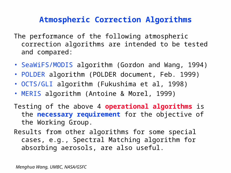
The performance of the following atmospheric correction algorithms are intended to be tested and compared:

• SeaWiFS/MODIS algorithm (Gordon and Wang, 1994)

• POLDER algorithm (POLDER document, Feb. 1999)

• OCTS/GLI algorithm (Fukushima et al, 1998)

• MERIS algorithm (Antoine & Morel, 1999)

Testing of the above 4 operational algorithms is the necessary requirement for the objective of the Working Group.

Results from other algorithms for some special cases, e.g., Spectral Matching algorithm for absorbing aerosols, are also useful.


Parameters

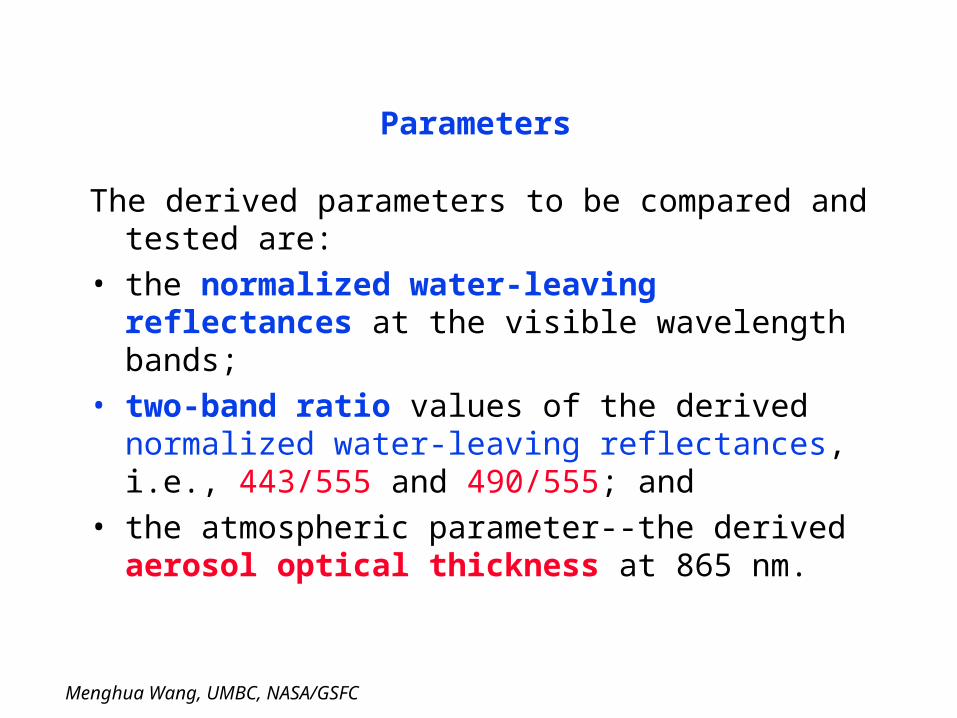
The derived parameters to be compared and tested are:

• the normalized water-leaving reflectances at the visible wavelength bands;

• two-band ratio values of the derived normalized water-leaving reflectances, i.e., 443/555 and 490/555; and

• the atmospheric parameter--the derived aerosol optical thickness at 865 nm.


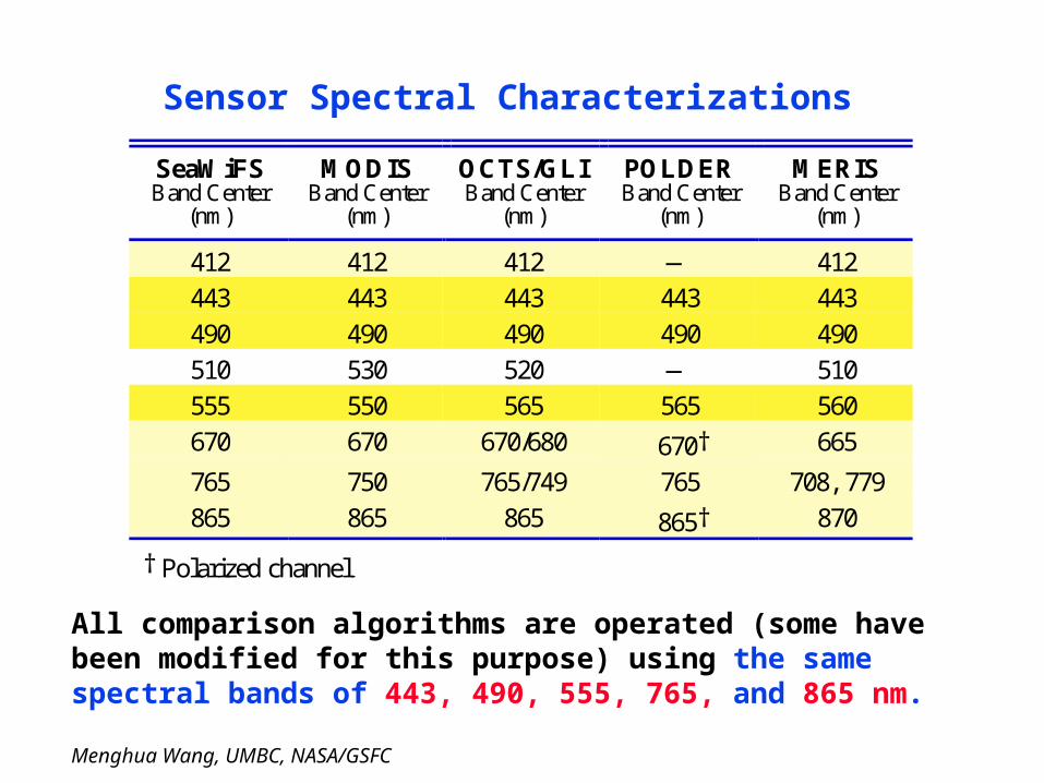
Sensor Spectral Characterizations

SeaWiFSBand Center

(nm)

MODISBand Center

(nm)

OCTS/GLIBand Center

(nm)

POLDERBand Center

(nm)

MERISBand Center

(nm)

412 412 412 — 412

443 443 443 443 443

490 490 490 490 490

510 530 520 — 510

555 550 565 565 560

670 670 670/680 670† 665

765 750 765/749 765 708, 779

865 865 865 865† 870

† Polarized channel.

All comparison algorithms are operated (some have been modified for this purpose) using the same spectral bands of 443, 490, 555, 765, and 865 nm.


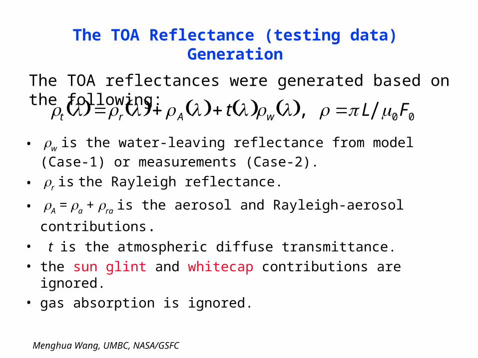
The TOA Reflectance (testing data) Generation

• w is the water-leaving reflectance from model (Case-1) or

measurements (Case-2).

• r is the Rayleigh reflectance.

• A = a + ra is the aerosol and Rayleigh-aerosol contributions.• t is the atmospheric diffuse transmittance.

• the sun glint and whitecap contributions are ignored.

• gas absorption is ignored.

The TOA reflectances were generated based on the following:

t r A t w , L 0 F0


Testing Data Sets

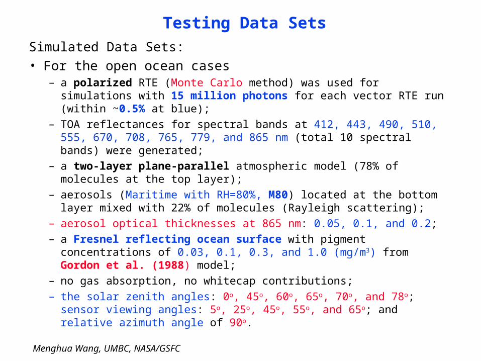
Simulated Data Sets:

• For the open ocean cases – a polarized RTE (Monte Carlo method) was used for simulations with

15 million photons for each vector RTE run (within ~0.5% at blue);

– TOA reflectances for spectral bands at 412, 443, 490, 510, 555, 670, 708, 765, 779, and 865 nm (total 10 spectral bands) were generated;

– a two-layer plane-parallel atmospheric model (78% of molecules at the top layer);

– aerosols (Maritime with RH=80%, M80) located at the bottom layer mixed with 22% of molecules (Rayleigh scattering);

– aerosol optical thicknesses at 865 nm: 0.05, 0.1, and 0.2;

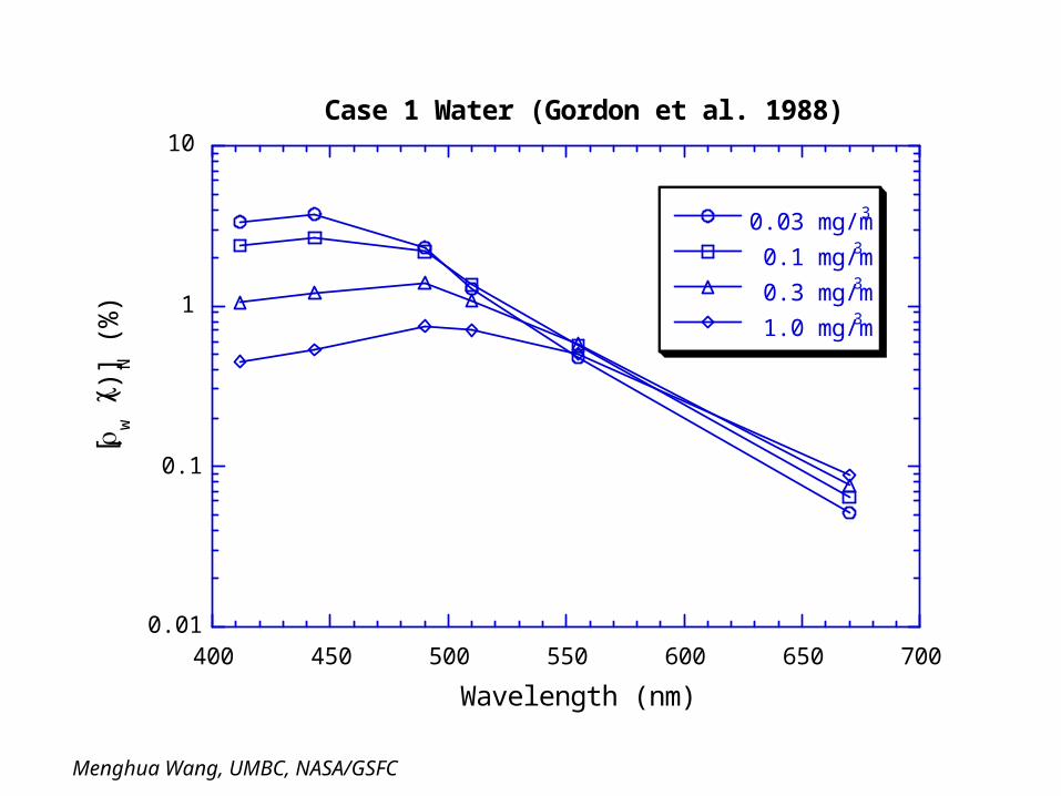
– a Fresnel reflecting ocean surface with pigment concentrations of 0.03, 0.1, 0.3, and 1.0 (mg/m3) from Gordon et al. (1988) model;

– no gas absorption, no whitecap contributions;

– the solar zenith angles: 0o, 45o, 60o, 65o, 70o, and 78o; sensor viewing angles: 5o, 25o, 45o, 55o, and 65o; and relative azimuth angle of 90o.


-0.2

-0.1

0

0.1

0.2

0 10 20 30 40 50 60 70

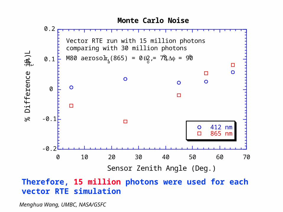
Monte Carlo Noise

412 nm865 nm

% D

iffe

ren

ce in

Lt(

)

Sensor Zenith Angle (Deg.)

M80 aerosol, a(865) = 0.2,

o = 78o, = 90o

Vector RTE run with 15 million photonscomparing with 30 million photons

Therefore, 15 million photons were used for each vector RTE simulation


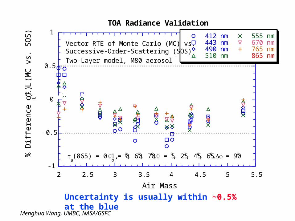
Uncertainty is usually within ~0.5% at the blue

-1

-0.5

0

0.5

1

2 2.5 3 3.5 4 4.5 5 5.5

TOA Radiance Validation

412 nm443 nm490 nm510 nm

555 nm670 nm765 nm865 nm

% D

iffe

ren

ce o

f L t(

) (M

C v

s. S

OS

)

Air Mass

Vector RTE of Monte Carlo (MC) vs. Successive-Order-Scattering (SOS)

Two-Layer model, M80 aerosol

a(865) = 0.1,

o = 0o, 60o, 70o, = 5o, 25o, 45o, 65o, = 90o


Testing Data Sets (cont.)

• Some cases for sensitivity studies (simulated data sets)– absorbing aerosols: Urban aerosols with two type vertical distributions,

i.e., two-layer and uniformly mixed one-layer cases;

– case 2 water—although algorithms are mostly intended for case 1 water, a quantitative estimation of atmospheric correction error over case 2 water is needed.

Data from SeaWiFS measurements (this is still open….):– open ocean cases (with various locations and seasons);

– coastal region ocean waters;

– some trouble cases, e.g., nLw<0, dust contamination, etc.

For testing and comparison, SeaWiFS data sets are usually co-located with in situ measurements. It was agreed that SeaDAS will be used.


Diffuse Transmittance Issue

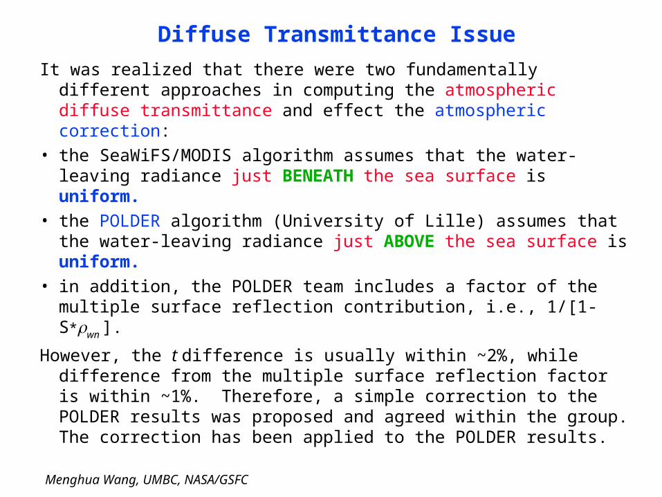
It was realized that there were two fundamentally different approaches in computing the atmospheric diffuse transmittance and effect the atmospheric correction:

• the SeaWiFS/MODIS algorithm assumes that the water-leaving radiance just BENEATH the sea surface is uniform.

• the POLDER algorithm (University of Lille) assumes that the water-leaving radiance just ABOVE the sea surface is uniform.

• in addition, the POLDER team includes a factor of the multiple surface reflection contribution, i.e., 1/[1-S*wn ].

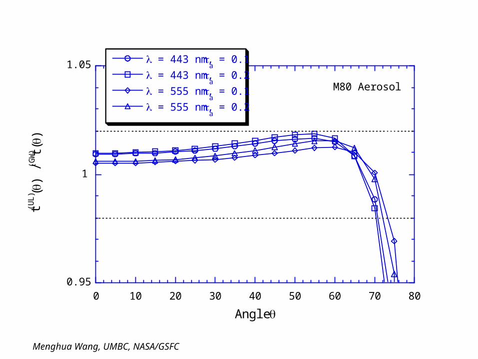
However, the t difference is usually within ~2%, while difference from the multiple surface reflection factor is within ~1%. Therefore, a simple correction to the POLDER results was proposed and agreed within the group. The correction has been applied to the POLDER results.


0.95

1

1.05

0 10 20 30 40 50 60 70 80

= 443 nm, a = 0.1

= 443 nm, a = 0.2

= 555 nm, a = 0.1

= 555 nm, a = 0.2

t(UL)

()

/ t(G

W) (

)

Angle

M80 Aerosol


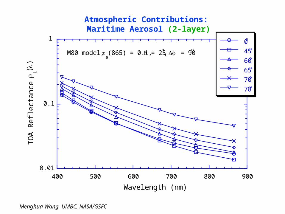
0.01

0.1

1

400 500 600 700 800 900

0o

45o

60o

65o

70o

78o

TO

A R

efl

ect

an

ce

t()

Wavelength (nm)

M80 model, a(865) = 0.1, = 25

o, = 90

o

Atmospheric Contributions: Maritime Aerosol (2-layer)


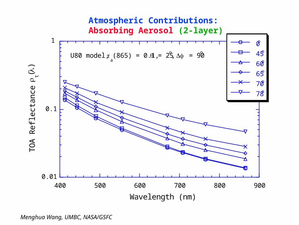
0.01

0.1

1

400 500 600 700 800 900

0o

45o

60o

65o

70o

78o

TO

A R

efl

ect

an

ce

t()

Wavelength (nm)

U80 model, a(865) = 0.1, = 25

o, = 90

o

Atmospheric Contributions: Absorbing Aerosol (2-layer)


0.01

0.1

1

10

400 450 500 550 600 650 700

Case 1 Water (Gordon et al. 1988)

0.03 mg/m3

0.1 mg/m3

0.3 mg/m3

1.0 mg/m3

[w ( )

] N (%

)

Wavelength (nm)


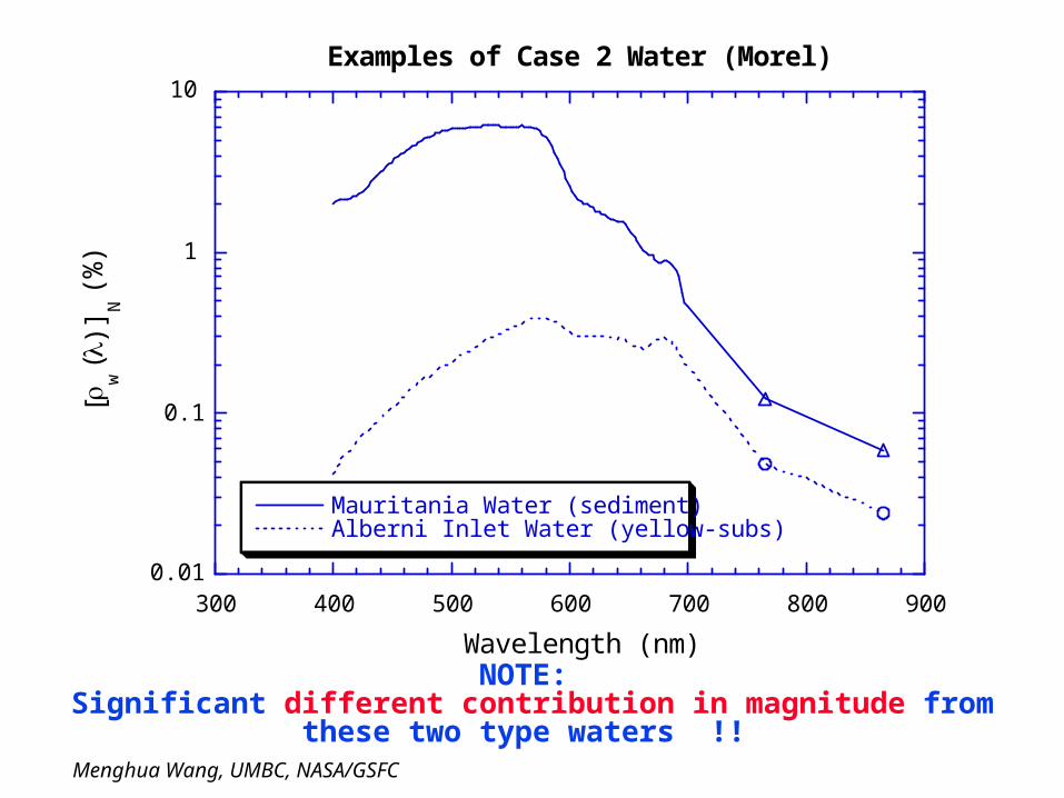
0.01

0.1

1

10

300 400 500 600 700 800 900

Examples of Case 2 Water (Morel)

Mauritania Water (sediment)Alberni Inlet Water (yellow-subs)

[w(

)] N

(%

)

Wavelength (nm)

NOTE: Significant different contribution in magnitude from these two type waters !!


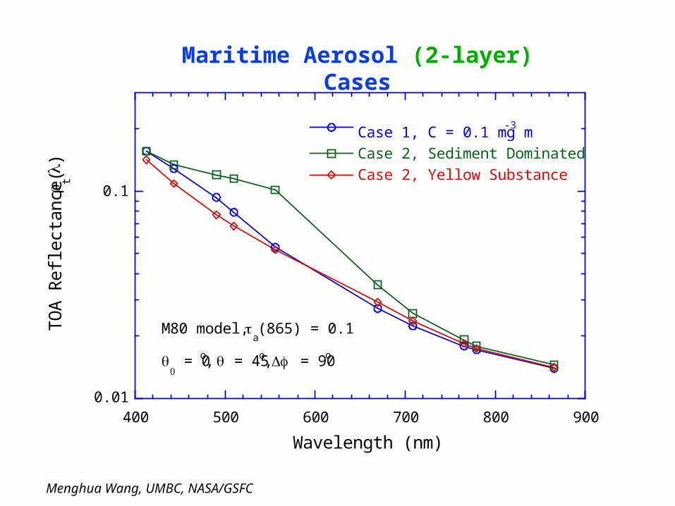
0.01

0.1

400 500 600 700 800 900

Case 1, C = 0.1 mg m-3

Case 2, Sediment Dominated

Case 2, Yellow Substance

TO

A R

efle

cta

nce

t(

)

Wavelength (nm)

M80 model, a(865) = 0.1

= 0o, = 45o, = 90o

Maritime Aerosol (2-layer) Cases


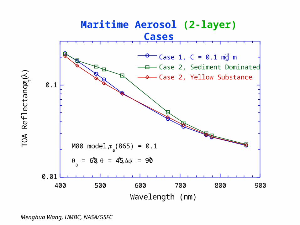
0.01

0.1

400 500 600 700 800 900

Case 1, C = 0.1 mg m-3



TO

A R

efle

cta

nce

t(

)

Wavelength (nm)

M80 model, a(865) = 0.1

= 60o, = 45o, = 90o

Maritime Aerosol (2-layer) Cases


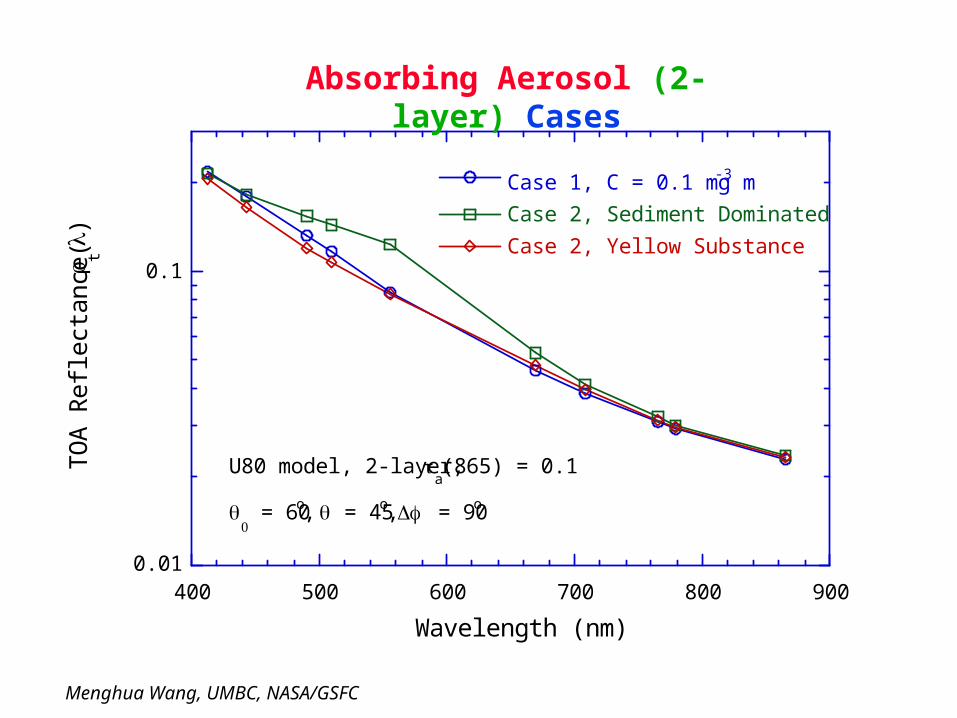
0.01

0.1

400 500 600 700 800 900

Case 1, C = 0.1 mg m-3



TO

A R

efle

cta

nce

t(

)

Wavelength (nm)

U80 model, 2-layer, a(865) = 0.1

= 60o, = 45o, = 90o

Absorbing Aerosol (2-layer) Cases


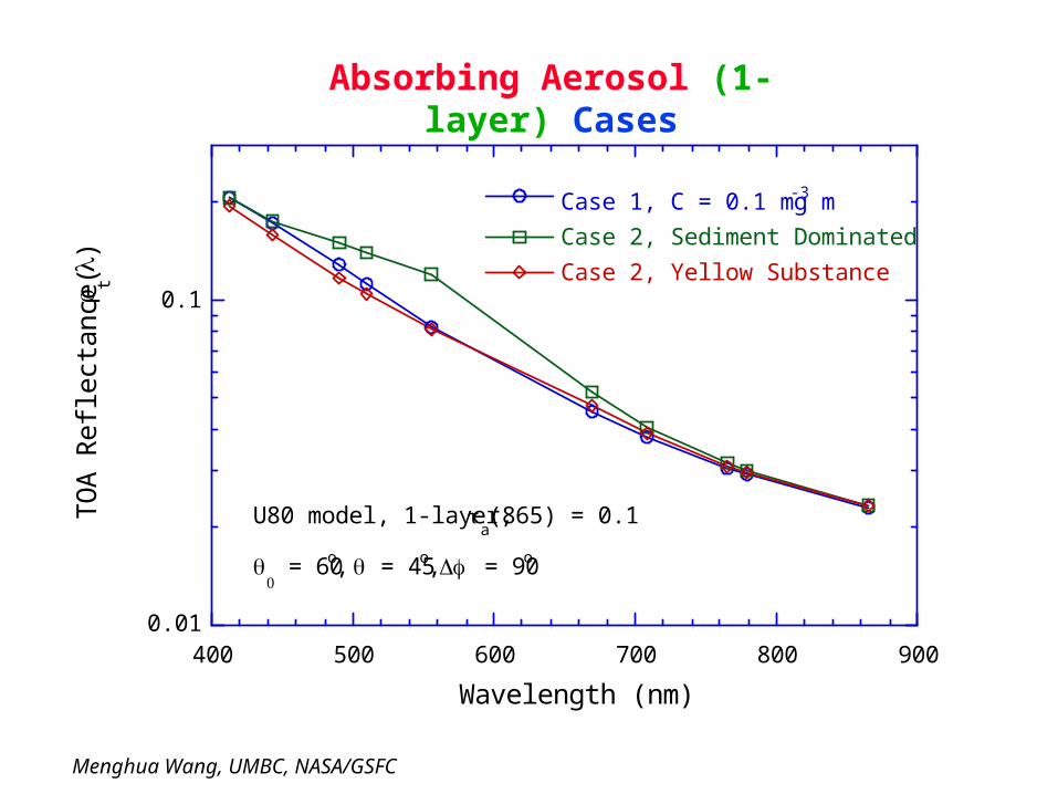
0.01

0.1

400 500 600 700 800 900

Case 1, C = 0.1 mg m-3



TO

A R

efle

cta

nce

t(

)

Wavelength (nm)

U80 model, 1-layer, a(865) = 0.1

= 60o, = 45o, = 90o

Absorbing Aerosol (1-layer) Cases


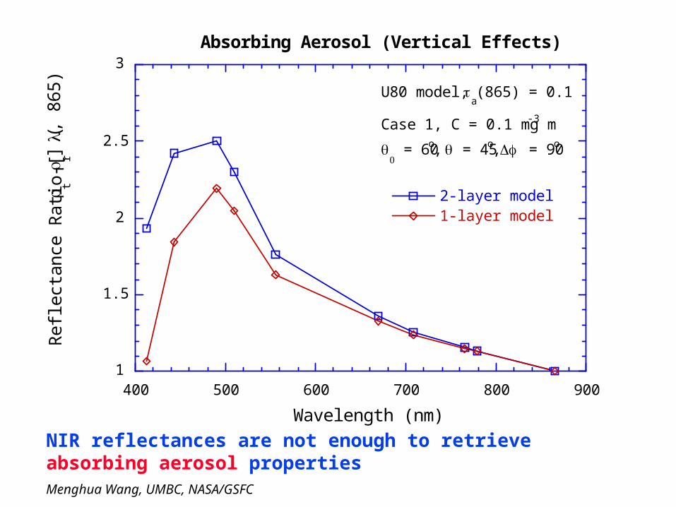
1

1.5

2

2.5

3

400 500 600 700 800 900

Absorbing Aerosol (Vertical Effects)

2-layer model1-layer model

Re

flect

an

ce R

atio

[t -

r]

(,

86

5)

Wavelength (nm)

U80 model, a(865) = 0.1

Case 1, C = 0.1 mg m-3

= 60o, = 45o, = 90o

NIR reflectances are not enough to retrieve absorbing aerosol properties


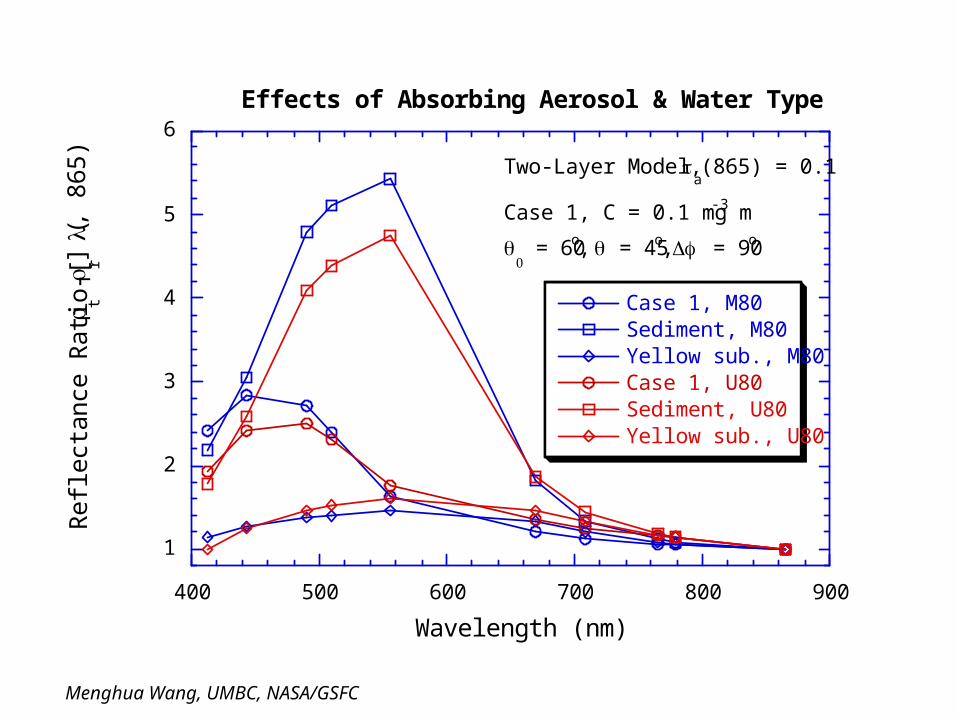
1

2

3

4

5

6

400 500 600 700 800 900

Effects of Absorbing Aerosol & Water Type

Case 1, M80Sediment, M80Yellow sub., M80Case 1, U80Sediment, U80Yellow sub., U80

Re

flect

an

ce R

atio

[t -

r]

(,

86

5)

Wavelength (nm)

Two-Layer Model, a(865) = 0.1

Case 1, C = 0.1 mg m-3

= 60o, = 45o, = 90o


ALL COMPARISON RESULTS ARE PRELIMINARY!


WORK IS IN PROGRESS …….


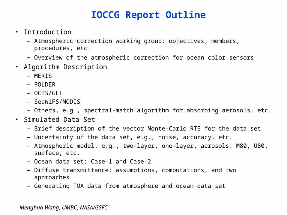
IOCCG Report Outline

• Introduction– Atmospheric correction working group: objectives, members, procedures, etc.

– Overview of the atmospheric correction for ocean color sensors

• Algorithm Description– MERIS

– POLDER

– OCTS/GLI

– SeaWiFS/MODIS

– Others, e.g., spectral-match algorithm for absorbing aerosols, etc.

• Simulated Data Set– Brief description of the vector Monte-Carlo RTE for the data set

– Uncertainty of the data set, e.g., noise, accuracy, etc.

– Atmospheric model, e.g., two-layer, one-layer, aerosols: M80, U80, surface, etc.

– Ocean data set: Case-1 and Case-2

– Diffuse transmittance: assumptions, computations, and two approaches

– Generating TOA data from atmosphere and ocean data set


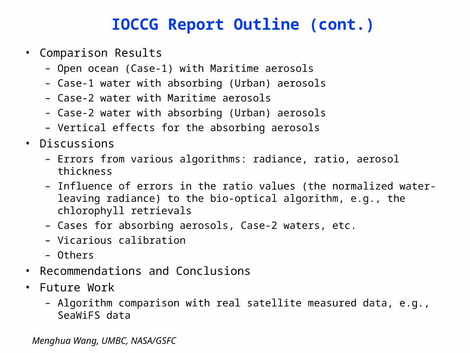
IOCCG Report Outline (cont.)

• Comparison Results– Open ocean (Case-1) with Maritime aerosols

– Case-1 water with absorbing (Urban) aerosols

– Case-2 water with Maritime aerosols

– Case-2 water with absorbing (Urban) aerosols

– Vertical effects for the absorbing aerosols

• Discussions– Errors from various algorithms: radiance, ratio, aerosol thickness

– Influence of errors in the ratio values (the normalized water-leaving radiance) to the bio-optical algorithm, e.g., the chlorophyll retrievals

– Cases for absorbing aerosols, Case-2 waters, etc.

– Vicarious calibration

– Others

• Recommendations and Conclusions

• Future Work– Algorithm comparison with real satellite measured data, e.g., SeaWiFS data


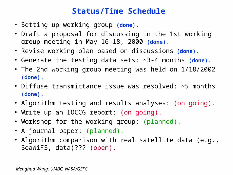
Status/Time Schedule

• Setting up working group (done).

• Draft a proposal for discussing in the 1st working group meeting in May 16-18, 2000 (done).

• Revise working plan based on discussions (done).

• Generate the testing data sets: ~3-4 months (done).

• The 2nd working group meeting was held on 1/18/2002 (done).

• Diffuse transmittance issue was resolved: ~5 months (done).

• Algorithm testing and results analyses: (on going).

• Write up an IOCCG report: (on going).

• Workshop for the working group: (planned).

• A journal paper: (planned).

• Algorithm comparison with real satellite data (e.g., SeaWiFS, data)??? (open).

Documents

Menghua Wang, UMBC, NASA/GSFC The IOCCG Atmospheric Correction Working Group Status Report The Eighth IOCCG Committee Meeting Department of Animal Biology