Meetings with Lambert W and Other Special

Functions in Optimization and Analysis

Jonathan M. BorweinCARMA

University of Newcastle

Scott B. LindstromCARMA

University of Newcastle

June 13, 2016

Abstract

We remedy the under-appreciated role of the Lambert W function inconvex analysis and optimization. We first discuss the role of little-knownspecial functions in optimization and then illustrate the relevance of Win a series problem posed by Donald Knuth. We then provide a basicoverview of the convex analysis of W and go on to explore its role induality theory where it appears quite naturally in the closed forms of theconvex conjugates for certain functions. We go on to discover a usefulclass of functions for which this is the case and investigate their use inoptimization, providing some code and examples.

1 Introduction

This paper and its accompanying lecture could be entitled “Meetings with Wand other too little known functions.” It is provided in somewhat of a tutorialform so as to allow us to meet a wider audience.

Throughout our discussion, we explain the role computer assistance played inour discoveries, with particular attention to our Maple package Symbolic ConvexAnalysis Tools and its numerical partner CCAT. We also note that, superficially,W provides an excellent counterexample to Stigler’s law of eponomy [25] whichstates that a scientific discovery is named after the last person to discover it.

For us, the Lambert W function is the real analytic inverse of x 7→ x exp(x).The real inverse is two-valued, as shown in Figure 1, while the complex inversehas countably many branches. We are interested in the principal branch. Thisis the analytic branch of W that has the following Taylor series

W(x) =

∞∑k=1

(−k)k−1

k!xk, (1)

with radius of convergence 1/e. This is the solution that reversion of the series(otherwise called the Lagrange inversion theorem) produces from x ·ex. Implicitdifferentiation leads to

W ′(x) =W (x)

x (1 +W (x)). (2)

1

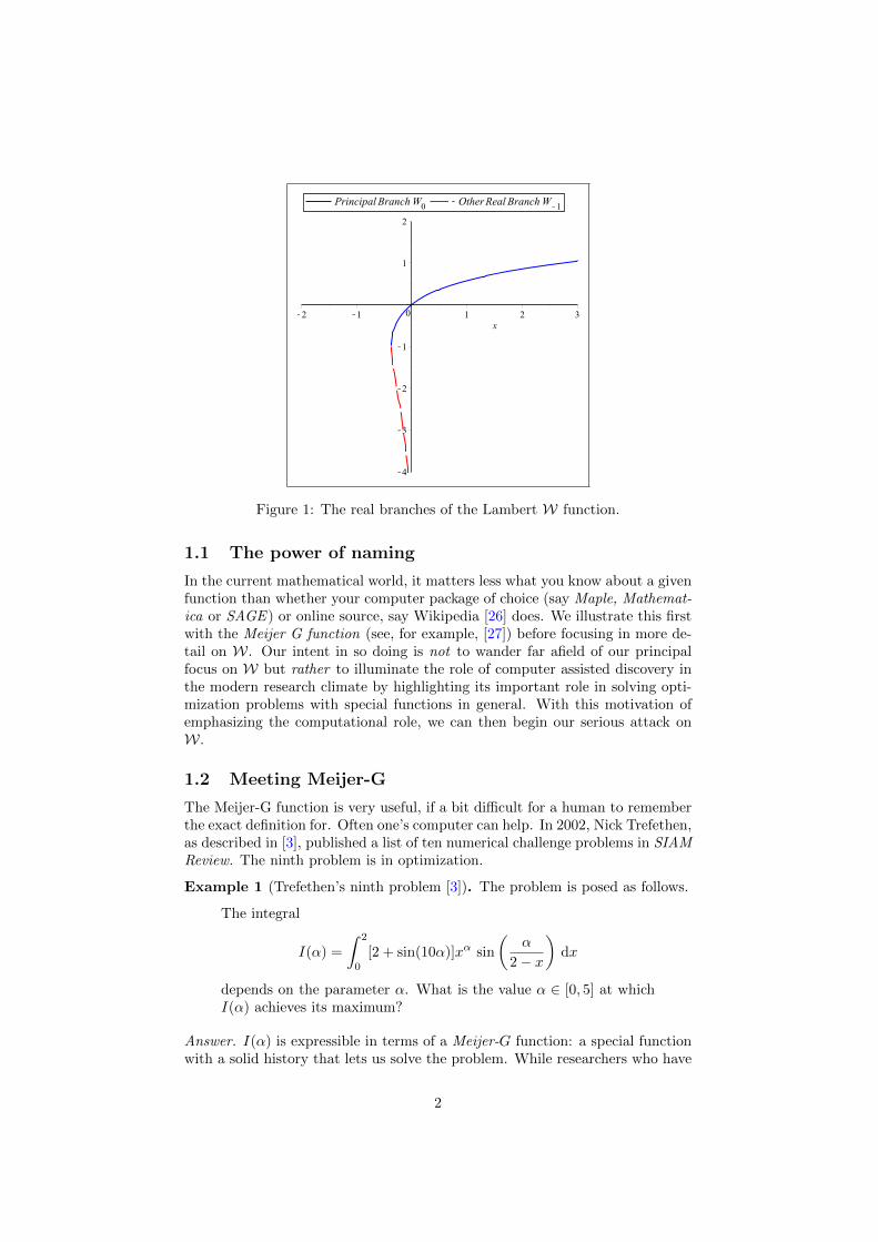
Figure 1: The real branches of the Lambert W function.

1.1 The power of naming

In the current mathematical world, it matters less what you know about a givenfunction than whether your computer package of choice (say Maple, Mathemat-ica or SAGE ) or online source, say Wikipedia [26] does. We illustrate this firstwith the Meijer G function (see, for example, [27]) before focusing in more de-tail on W. Our intent in so doing is not to wander far afield of our principalfocus on W but rather to illuminate the role of computer assisted discovery inthe modern research climate by highlighting its important role in solving opti-mization problems with special functions in general. With this motivation ofemphasizing the computational role, we can then begin our serious attack onW.

1.2 Meeting Meijer-G

The Meijer-G function is very useful, if a bit difficult for a human to rememberthe exact definition for. Often one’s computer can help. In 2002, Nick Trefethen,as described in [3], published a list of ten numerical challenge problems in SIAMReview. The ninth problem is in optimization.

Example 1 (Trefethen’s ninth problem [3]). The problem is posed as follows.

The integral

I(α) =

∫ 2

0

[2 + sin(10α)]xα sin

(α

2− x

)dx

depends on the parameter α. What is the value α ∈ [0, 5] at whichI(α) achieves its maximum?

Answer. I(α) is expressible in terms of a Meijer-G function: a special functionwith a solid history that lets us solve the problem. While researchers who have

2

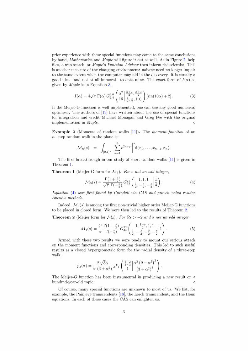
prior experience with these special functions may come to the same conclusionsby hand, Mathematica and Maple will figure it out as well. As in Figure 2, helpfiles, a web search, or Maple’s Function Advisor then inform the scientist. Thisis another measure of the changing environment: naivete need no longer impairto the same extent when the computer may aid in the discovery. It is usually agood idea—and not at all immoral—to data mine. The exact form of I(α) asgiven by Maple is in Equation 3.

I(α) = 4√π Γ(α)G3,0

2,4

(α2

16

∣∣∣∣ α+22 , α+3

212 ,

12 , 1, 0

)[sin(10α) + 2] . (3)

If the Meijer-G function is well implemented, one can use any good numericaloptimiser. The authors of [19] have written about the use of special functionsfor integration and credit Michael Monagan and Greg Fee with the originalimplementation in Maple. �

Example 2 (Moments of random walks [11]). The moment function of ann−step random walk in the plane is:

Mn(s) =

∫[0,1]n

∣∣∣∣ n∑k=1

e2πxki∣∣∣∣sd(x1, . . . , xn−1, xn).

The first breakthrough in our study of short random walks [11] is given inTheorem 1.

Theorem 1 (Meijer-G form for M3). For s not an odd integer,

M3(s) =Γ(1 + s

2 )√π Γ(− s2 )

G2133

(1, 1, 1

12 ,−

s2 ,−

s2

∣∣∣∣14). (4)

Equation (4) was first found by Crandall via CAS and proven using residuecalculus methods.

Indeed,M3(s) is among the first non-trivial higher order Meijer-G functionsto be placed in closed form. We were then led to the results of Theorem 2.

Theorem 2 (Meijer form for M4). For <s > −2 and s not an odd integer

M4(s) =2s

π

Γ(1 + s2 )

Γ(− s2 )G22

44

(1, 1−s2 , 1, 1

12 −

s2 ,−

s2 ,−

s2

∣∣∣∣1). (5)

Armed with these two results we were ready to mount our serious attackon the moment functions and corresponding densities. This led to such usefulresults as a closed hypergeometric form for the radial density of a three-stepwalk:

p3(α) =2√

3α

π (3 + α2)2F1

(13 ,

23

1

∣∣∣∣α2(9− α2

)2(3 + α2)

3

).

The Meijer-G function has been instrumental in producing a new result on ahundred-year-old topic. �

Of course, many special functions are unknown to most of us. We list, forexample, the Painleve transcendents [18], the Lerch transcendent, and the Heunequations. In each of these cases the CAS can enlighten us.

3

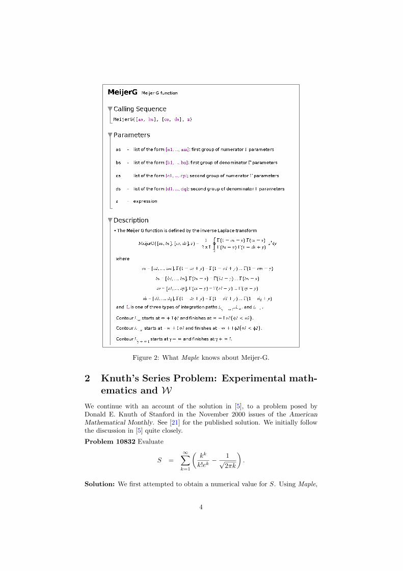
Figure 2: What Maple knows about Meijer-G.

2 Knuth’s Series Problem: Experimental math-ematics and W

We continue with an account of the solution in [5], to a problem posed byDonald E. Knuth of Stanford in the November 2000 issues of the AmericanMathematical Monthly. See [21] for the published solution. We initially followthe discussion in [5] quite closely.

Problem 10832 Evaluate

S =

∞∑k=1

(kk

k!ek− 1√

2πk

).

Solution: We first attempted to obtain a numerical value for S. Using Maple,

4

Figure 3: The complex moment functionM4 as drawn from (5) in the CalendarComplex Beauties 2016.

we produced the approximation

S ≈ −0.08406950872765599646.

Based on this numerical value, the Inverse Symbolic Calculator, available atthe URL http://isc.carma.newcastle.edu.au/, with the “Smart Lookup”feature, yielded the result

S ≈ −2

3− 1√

2πζ

(1

2

).

Calculations to even higher precision (50 decimal digits) confirmed this approx-imation. Thus within a few minutes we “knew” the answer.

Why should such an identity hold? One clue was provided by the surprisingspeed with which Maple was able to calculate a high-precision value of thisslowly convergent infinite sum. Evidently, the Maple software knew somethingthat we did not. Peering under the hood, we found that Maple was using theLambert W function, which, as we know, is the functional inverse of z → zez.

Another clue was the appearance of ζ(1/2) in the above experimental iden-tity, together with an obvious allusion to Stirling’s formula in the original prob-lem. This led us to conjecture the identity

∞∑k=1

(1√2πk

− (1/2)k−1

(k − 1)!√

2

)=

1√2πζ

(1

2

),

where (x)n denotes x(x+ 1) · · · (x+ n− 1), we say “x to the n rising,”[20] andwhere the binomial coefficients in the LHS of (6) are the same as those of the

5

function 1/√

2− 2x. Moreover, Maple successfully evaluated this summation,as shown on the RHS and as is further discussed in Remark 1. We now neededto establish that

∞∑k=1

(kk

k!ek− (1/2)k−1

(k − 1)!√

2

)= −2

3.

Guided by the presence of the Lambert W function, as in (1),

W(z) =

∞∑k=1

(−k)k−1zk

k!,

an appeal to Abel’s limit theorem suggested the conjectured identity

limz→1

(dW(−z/e)

dz+

1√2− 2z

)=

2

3. (6)

Here again, Maple was able to evaluate this limit and establish the identity (6)which relies on the following reversion [16]. Let p =

√2(1 + ez) with z =WeW ,

so that

p2

2− 1 =W exp(1 +W) = −1 +

∑k≥1

(1

k!− 1

(k − 1)!

)(1 +W)k

and revert to

1 +W = p− p2

3+

11

72p3 + . . .

for |p| <√

2. Now (2) lets us prove (6).As can be seen from this account, the above manipulation took considerable

human ingenuity, in addition to computer-based symbolic manipulation. Weinclude this example to highlight a challenge for the next generation of math-ematical computing software—these tools need to more completely automatethis class of operations, so that similar derivations can be accomplished by asignificantly broader segment of the mathematical community.

Remark 1 (ζ(s) for 0 < s < ∞, s 6= 1). More generally, for 0 < Re s < 1 inthe complex plane, we discovered empirically that

∞∑k=1

(1

ks− Γ (k − s)

Γ (k)

)= ζ (s) .

Now Maple’s summation tools can reduce this to

N∑k=1

1

ks− Γ (N + 1− s)

(1− s) Γ (N)→ ζ(s).

For any given rational s ∈ (0,∞) Maple will evaluate the limit by the Euler-Maclaurin method. Consulting the DLMF at http://dlmf.nist.gov/25.2#E8we discover

ζ(s) =

N∑k=1

1

ks+N1−s

s− 1− s

∫ ∞N

x− bxcxs+1

dx.

6

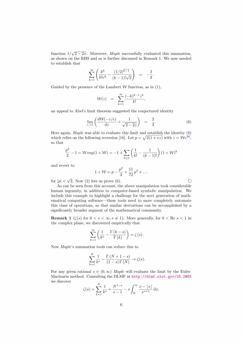
Figure 4: The function κ to the left and right of s = 1/2..

Since the integral tends to zero for s > 0 and

limN→∞

Γ (N + 1− s)(1− s) Γ (N)

− N1−s

1− s= 0,

we can also produce an explicit human proof. �We end this section with an open question:

Question 1. Can one find an extension of (6) for general s 6= 1/2 in (0, 1)?Based on (7) and the Stirling approximation for Γ(k + s) ≈

√2π e−kkk+s−1/2

we obtain∞∑k=1

(1√

2πks− kk+1/2−s

k! ek

)− ζ (s)√

2π= κ (s) .

We have that κ(1/2) = 2/3, but it remains to evaluate κ(s) ∈ R more generally,as drawn in Figure 4.

For s 6= 1/2 we have not found an analogue to (6), and there is no reason tobe sure such an analog exists. Numerically to 25 places we record:

κ(1/3) = 0.5051265122136281644488407

κ(2/3) = 1.044357456635617976159955

κ(1/4) = 0.4742404657846664773555294

κ(3/4) = 1.435469800298317747887340

κ(1/6) = 0.4899050094518209209997454

κ(5/6) = 2.226651254233652670106746.

Thus our question is closely allied to that of asking whether

W(x; s) =

∞∑k=1

kk+1/2−s

k!xk

for s 6= 1/2, can be analysed in terms of W.

7

3 The convex analysis of W (as a real function)

The Maple package Symbolic Convex Analysis Tools, or SCAT, which performsconvex analysis symbolically, and its partner CCAT (which performs convexanalysis numerically) are described in [7] and are available together at http://carma.newcastle.edu.au/ConvexFunctions/SCAT.ZIP. We refer to [8, 12, 14]for any background convex analysis not discussed herein.

3.1 Basic properties

1. W is concave on (−1/e,∞) and positive on (0,∞).

2. (log ◦W)(z) = log(z)−W(z) is concave, as W is log concave on (0,∞).

3. (exp ◦W)(z) = z/W(z) is concave.

In order to prove these, we will make use of the following lemma, which isquite convenient.

Lemma 3. An invertible real valued function f with domain X ⊂ R is concaveif its inverse function f−1 is convex and monotone increasing on its domainf−1(X).

Proof. Other variations of this result are readily available (see, for example,[24]), and it is often left as an exercise in texts (see, for example, [15, Exercise3.3]). Let x, y ∈ X. By the bijectivity of the function f , there exist u, v suchthat f−1(u) = x and f−1(v) = y. Thus we have that

f(λx+ (1− λ)y) = f(λf−1(u) + (1− λ)f−1(v)).

By the convexity of f−1, we have that

λf−1(u) + (1− λ)f−1(v) ≤ f−1(λu+ +(1− λ)v) (7)

Since f−1 is monotone increasing, f is monotone increasing. Using this facttogether with Equation 7 shows that

f(λf−1(u) + (1− λ)f−1(v)) ≤ f(f−1(λu+ +(1− λ)v)) = λu+ (1− λ)v. (8)

Finally, we haveλu+ (1− λ)v = λf(x) + (1− λ)f(y).

This result greatly simplifies the following propositions.

Corollary 4. An invertible real valued function f with domain X ⊂ R is con-cave if its inverse function f−1 is convex and monotone decreasing on its domainf−1(X).

Proof. The proof is the same as that of Lemma 3 with the exception that thedirection of the inequality is reversed in Equation (8) beause the inverse is nowdecreasing instead of increasing.

Proposition 5. W is concave on (−1/e,∞).

8

Proof. Notice that W−1(( 1e ,∞)) = (−1,∞). By Lemma 3, it suffices to show

that the inverse of W is convex and monotone increasing on (−1,∞). Sincethe inverse of W is xex, we differentiate; the convexity and monotonicity areclear from the fact that the first two derivatives are both positive on the entiredomain.

Definition 1. A function f is called logarithmically concave if it is strictlygreater than zero on its domain and log ◦f is concave. Similarly f is calledlogarithmically convex if it is strictly greater than zero on its domain and log ◦fis convex.[15]

Remark 2. The function (log ◦W)(z) = log(z) − W(z) is concave. This istrue since W is concave and its restriction to (0,∞) = dom(log ◦W) is strictlygreater than zero everywhere.

Proposition 6. The function given by (exp ◦W)(x) = x/W(x) is concave.

Proof. Consider the inverse of this function

log(x)elog(x) = x log(x).

Again, by Lemma 3, it suffices to show that this function is convex and monotoneincreasing on its domain ( 1

e ,∞). Differentiating, we again find that both thefirst and second derivatives are strictly greater than zero, showing the result.

Proposition 7. (exp ◦(−W))(x) =W(x)/x is convex.

Proof. By Corollary 4, it suffices to show that the inverse function

− log(x)e− log(x) = − log(x)/x

is convex and decreasing on its domain (0, e). Indeed, on this interval thefirst derivative is always negative and the second always positive, showing bothtraits.

3.2 The convex conjugate

The convex conjugate — or Fenchel–Moreau–Rockafellar conjugate or dual func-tion — plays much the role in convex analysis and optimization that the Fouriertransform plays in harmonic analysis. For a function f : X → [−∞,∞] we define

f∗ : X∗ → [−∞,∞] by (9)

f∗(y) = supx∈X{〈y, x〉 − f(x)}.

The function f∗ is always convex (if possibly always infinite), and if f is lowersemicontinuous, convex and proper then f∗∗ = f. In particular if we show afunction g = f∗ then g is necessarily convex.

Directly from (9) we have the Fenchel-Young inequality, for all y, x

f∗(y) + f(x) ≥ 〈y, x〉.

9

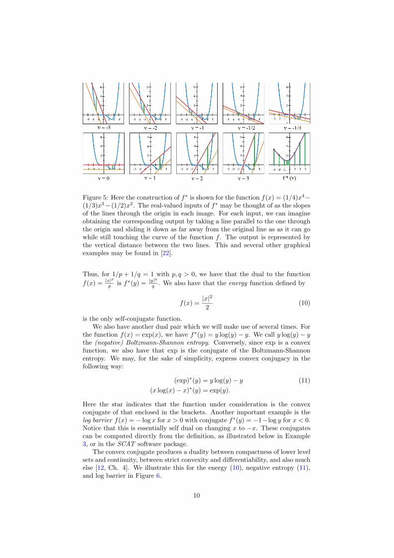
Figure 5: Here the construction of f∗ is shown for the function f(x) = (1/4)x4−(1/3)x3− (1/2)x2. The real-valued inputs of f∗ may be thought of as the slopesof the lines through the origin in each image. For each input, we can imagineobtaining the corresponding output by taking a line parallel to the one throughthe origin and sliding it down as far away from the original line as as it can gowhile still touching the curve of the function f . The output is represented bythe vertical distance between the two lines. This and several other graphicalexamples may be found in [22].

Thus, for 1/p + 1/q = 1 with p, q > 0, we have that the dual to the function

f(x) = |x|pp is f∗(y) = |y|q

q . We also have that the energy function defined by

f(x) =|x|2

2(10)

is the only self-conjugate function.We also have another dual pair which we will make use of several times. For

the function f(x) = exp(x), we have f∗(y) = y log(y)− y. We call y log(y)− ythe (negative) Boltzmann-Shannon entropy. Conversely, since exp is a convexfunction, we also have that exp is the conjugate of the Boltzmann-Shannonentropy. We may, for the sake of simplicity, express convex conjugacy in thefollowing way:

(exp)∗(y) = y log(y)− y (11)

(x log(x)− x)∗(y) = exp(y).

Here the star indicates that the function under consideration is the convexconjugate of that enclosed in the brackets. Another important example is thelog barrier f(x) = − log x for x > 0 with conjugate f∗(y) = −1− log y for x < 0.Notice that this is essentially self dual on changing x to −x. These conjugatescan be computed directly from the definition, as illustrated below in Example3, or in the SCAT software package.

The convex conjugate produces a duality between compactness of lower levelsets and continuity, between strict convexity and differentiability, and also muchelse [12, Ch. 4]. We illustrate this for the energy (10), negative entropy (11),and log barrier in Figure 6.

10

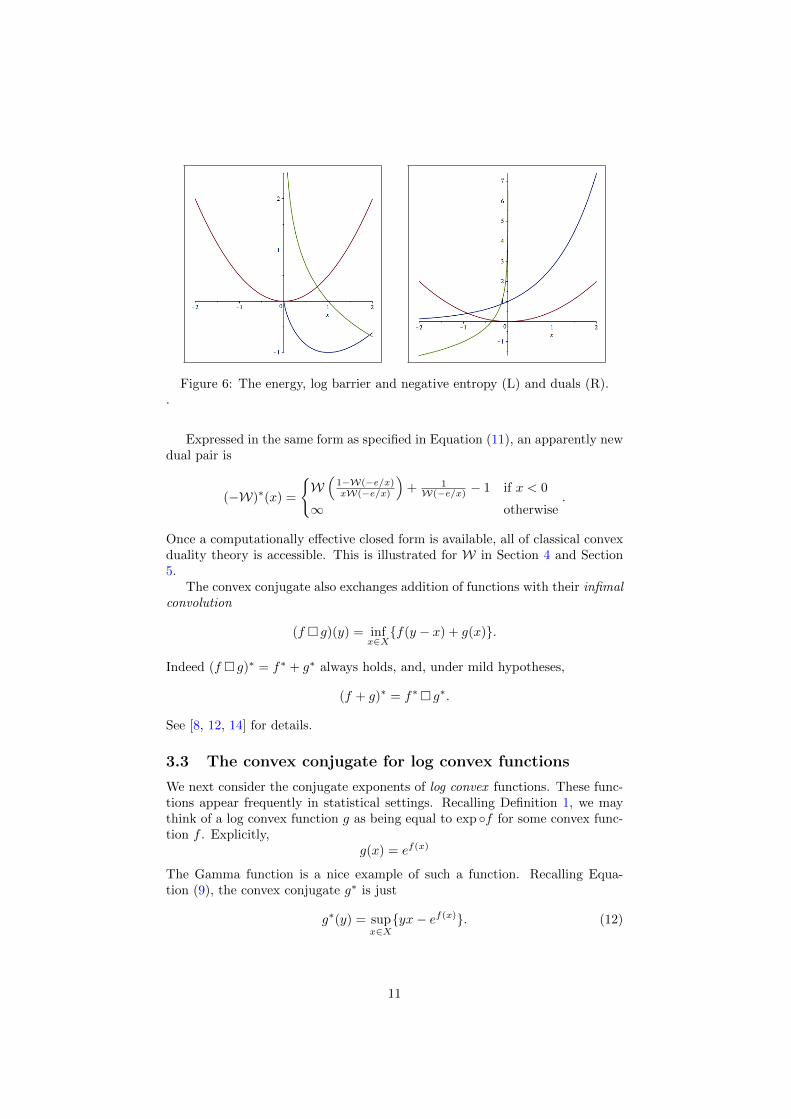
Figure 6: The energy, log barrier and negative entropy (L) and duals (R)..

Expressed in the same form as specified in Equation (11), an apparently newdual pair is

(−W)∗(x) =

{W(

1−W(−e/x)xW(−e/x)

)+ 1W(−e/x) − 1 if x < 0

∞ otherwise.

Once a computationally effective closed form is available, all of classical convexduality theory is accessible. This is illustrated for W in Section 4 and Section5.

The convex conjugate also exchanges addition of functions with their infimalconvolution

(f � g)(y) = infx∈X{f(y − x) + g(x)}.

Indeed (f � g)∗ = f∗ + g∗ always holds, and, under mild hypotheses,

(f + g)∗ = f∗� g∗.

See [8, 12, 14] for details.

3.3 The convex conjugate for log convex functions

We next consider the conjugate exponents of log convex functions. These func-tions appear frequently in statistical settings. Recalling Definition 1, we maythink of a log convex function g as being equal to exp ◦f for some convex func-tion f . Explicitly,

g(x) = ef(x)

The Gamma function is a nice example of such a function. Recalling Equa-tion (9), the convex conjugate g∗ is just

g∗(y) = supx∈X{yx− ef(x)}. (12)

11

By differentiating the inner term yx−ef(x) and setting equal to zero to find thepoint at which the function is maximized, we obtain

y = f ′(x)ef(x). (13)

If we can solve this equation for x = s(y), we will be able to write the conjugatefunction more clearly as

g∗(y) = y · s(y)− g(s(y))

How nice the answer is depends on how well this expression simplifies.

Example 3. A first and lovely example is:

(exp ◦ exp)∗

(y) =

y (log y −W(y)− 1/W(y)) y > 0

−1 y = 0

∞ y < 0

We will deduce this in the way described above. �

Starting from the definition,

g∗(y) = supx∈R{yx− ee

x

},

we take the derivative of the inner term on the right and set equal to zero toobtain

y = ex · eex

.

Notice that what we have here is just ex =W(y) and so we may actually solvefor x explicitly as follows:

x = (log ◦W)(y).

Thus we can substitute back into the original equation and have our closed formsolution

g∗(y) = y · (log ◦W)(y)− eW(y) = y(log(y)−W(y))− y/W (y). (14)

Example 4. A second example is related to the normal distribution. We take:

g(x) = ex2

2 for all x,

and we have that

g∗(y) = |y|

(√W(y2)− 1√

W(y2)

)for all y.

We derive this below. �

We can compute this result in the same way. Starting with the definition

g∗(y) = supx∈R{yx− e

(x2

2

)}. (15)

12

Differentiating and setting equal to zero, we obtain

y = x · e(x2

2

)(16)

Squaring both sides, we have y2 = x2 · ex2

. We can now see a way to use theLambert W function: x2 =W(y2). Thus we arrive at an expression for x:

x = sign(y) ·√W(y2).

This we can work with. If we instead asked Maple to solve Equation (16) for x,it gives us the solution

x = y · e− 12W (y2).

We can easily check to see this is an equivalent expression. Recall, as first notedin Proposition 6, that (exp ◦W)(x) = x/W(x). Thus we may write

e−12W (y2) =

(eW(y2)

)− 12

=

(y2

W(y2)

)− 12

=

√W(y2)

y2=

√W(y2)

|y|.

Thus we have that

y · e− 12W (y2) = y ·

√W(y2)

|y|= sign(y)

√W(y2).

Since we have an expression for x in terms of y, we can substitute back into theoriginal formulation from Equation (15) to obtain our closed-form expression

g∗(y) = |y|√W(y2)− exp

(|W (y2)|

2

). (17)

We can simplify this even further. W(y2) is always positive since y2 is alwayspositive, so we can lose the absolute value signs in the right most term andfurther simplify it as follows:

exp

(|W (y2)|

2

)=√eW(y2) =

√y2

W(y2)= |y| 1√

W(y2)

Thus Equation (17) simplifies to

g∗(y) = |y|

(√W(y2)− 1√

W(y2)

). (18)

We can check this answer using SCAT. We ask Maple to compute

n1:=convert(exp((x^2)/2),PWF);Conj(n1,y);

which yields the answer {|y|W (y2)− 1√

W (y2)all(y).

This matches our solution for g∗(y) from Equation (18).

13

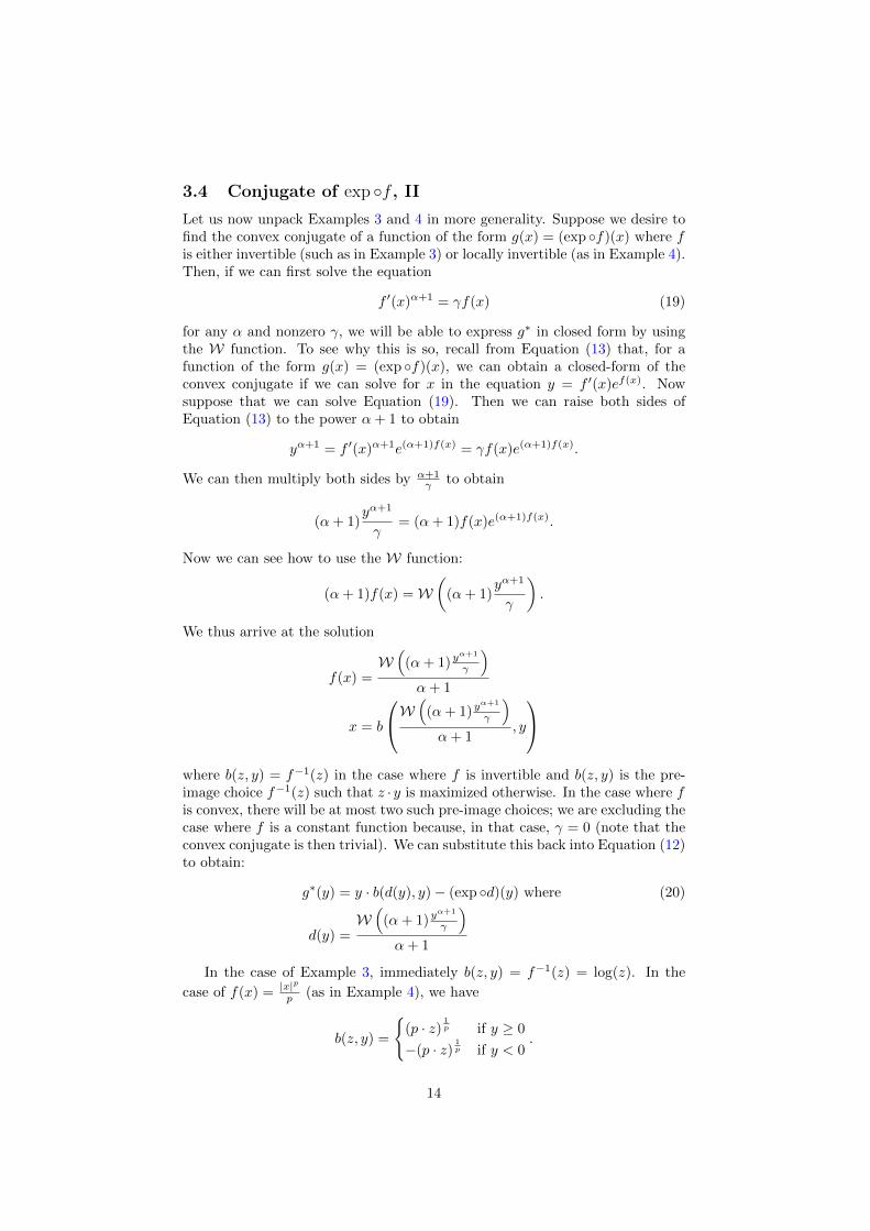
3.4 Conjugate of exp ◦f , II

Let us now unpack Examples 3 and 4 in more generality. Suppose we desire tofind the convex conjugate of a function of the form g(x) = (exp ◦f)(x) where fis either invertible (such as in Example 3) or locally invertible (as in Example 4).Then, if we can first solve the equation

f ′(x)α+1 = γf(x) (19)

for any α and nonzero γ, we will be able to express g∗ in closed form by usingthe W function. To see why this is so, recall from Equation (13) that, for afunction of the form g(x) = (exp ◦f)(x), we can obtain a closed-form of theconvex conjugate if we can solve for x in the equation y = f ′(x)ef(x). Nowsuppose that we can solve Equation (19). Then we can raise both sides ofEquation (13) to the power α+ 1 to obtain

yα+1 = f ′(x)α+1e(α+1)f(x) = γf(x)e(α+1)f(x).

We can then multiply both sides by α+1γ to obtain

(α+ 1)yα+1

γ= (α+ 1)f(x)e(α+1)f(x).

Now we can see how to use the W function:

(α+ 1)f(x) =W(

(α+ 1)yα+1

γ

).

We thus arrive at the solution

f(x) =W(

(α+ 1)yα+1

γ

)α+ 1

x = b

W(

(α+ 1)yα+1

γ

)α+ 1

, y

where b(z, y) = f−1(z) in the case where f is invertible and b(z, y) is the pre-image choice f−1(z) such that z ·y is maximized otherwise. In the case where fis convex, there will be at most two such pre-image choices; we are excluding thecase where f is a constant function because, in that case, γ = 0 (note that theconvex conjugate is then trivial). We can substitute this back into Equation (12)to obtain:

g∗(y) = y · b(d(y), y)− (exp ◦d)(y) where (20)

d(y) =W(

(α+ 1)yα+1

γ

)α+ 1

In the case of Example 3, immediately b(z, y) = f−1(z) = log(z). In the

case of f(x) = |x|pp (as in Example 4), we have

b(z, y) =

{(p · z)

1p if y ≥ 0

−(p · z)1p if y < 0

.

14

We can further simplify Equation (20) by again using the fact that (exp ◦W)(x) =x/W(x):

(exp ◦d)(y) = exp

(W(

(α+ 1)yα+1

γ

)) 1α+1

=

(α+ 1)yα+1

γ

W(

(α+ 1)yα+1

γ

) 1

α+1

.

Thus Equation (20) simplifies to

g∗(y) = y · b

W(

(α+ 1)yα+1

γ

)α+ 1

, y

− (α+ 1)y

α+1

γ

W(

(α+ 1)yα+1

γ

) 1

α+1

. (21)

Since this form is quite explicit, we may well ask for what kind of function f wecan solve Equation (19).

Here Maple is again useful, though a pencil-and-paper separation of variablescomputation will arrive at the same place. We use the built-in differentialequation solver dsolve, subject to appropriate conditions on the parametersf(0) = β,

dsolve({(diff(f(x), x))^(alpha+1) = gamma*f(x),f(0)=beta}, f(x))

and Maple provides the result

f (x) =

(1

α+ 1

(αxγ(α+1)−1

+ eα ln(β)α+1 α+ e

α ln(β)α+1

))α+1α

.

In the limit as α→ 0, Maple returns f(x) = β(exp(γx)) which we recognize asthe familiar form of Example 3. Also, if we let

α = 1, and γ = 2

and ask Maple for the limit as β approaches 0, we recover our familiar function

f(x) = x2

2 from Example 4. Thus, we have obtained a large class of closed forms

from which f(x) = β · exp(γx) (as in Example 3) and f(x) = |x|pp , (p > 1) (as in

Example 4) arise as special limiting cases. These are the two cases where thefinal closed forms of g∗ turn out to be particularly clean and pleasant.

We consider first the explicit closed form of the convex conjugates for func-tions of form β · exp(γx). Because g(γx) has convex conjugate g∗(xγ ) (see [8,

Table 3.2]), it suffices to simply show the form for the case γ = 1. In this case,α+ 1 = 1, so the form of the convex conjugate simplifies to

g∗(y) =

y(

log (y)−W (y)− 1W(y) − log(β)

)if y > 0

−1 if y = 0

∞ if y < 0

.

This can be easily compared to Equation (14) from Example 4 in which case wehad γ = 1. Indeed, the conjugate of βf(γx), β > 0 is always easily computedfrom that of f .

15

Turning our attention to functions of the general form f(x) = |x|pp , (p > 1),

we have that α+ 1 = pp−1 and γ = p, so Equation (21) becomes

g∗(y) = |y|

(

(p− 1)W

(|y|

pp−1

p− 1

)) 1p

−

1

(p− 1)W(|y|

pp−1

p−1

)

p−1p

. (22)

Compare this more general form of the convex conjugate to that for the specificcase p = 2 which we saw in Equation (18) from Example 4. We can also rewritethe convex conjugate using the conjugate exponent q. Where 1

q + 1p = 1, we

have q = pp−1 and p

q = p− 1, so Equation (22) becomes

g∗(y) = |y|

((p

qW(q

p|y|q)) 1

p

−(p

qW(q

p|y|q))− 1

q

). (23)

These simpler forms make the conjugates much easier to analyse and to compute.

Remark 3. Suppose f is variable separable. That is to say that

f(x1, x2, . . . , xn) =

n∑j=1

fj(xj)

where each fj is convex. Then f is convex and

f∗(y1, y2, . . . yn) =

n∑j=1

f∗j (yj).

From such building blocks and the Fenchel duality theorem [8, 12, 14] manyother convex conjugates engaging W are accessible.

The conjugate has many and diverse uses. For instance, one can establish theconvexity of a function through the smoothness of its conjugate. In Proposition 8we explore one such a situation which arises as a special case of [12, Cor 4.5.2].

Proposition 8. Suppose f : X → (−∞,+∞] is such that f∗∗ is proper. Supposef∗ is Frechet differentiable and f is lower semicontinuous. Then f is convex.

Example 5. We illustrate Proposition 8 for

f(x) = 2 |x| log (2 |x|)− 2 |x|+ 1

which has convex conjugate

f∗(y) =

{exp

(y2

)− 1 if y ≥ 0

exp(−y2)− 1 if y < 0

.

More simply, f∗(y) = exp(|y|/2) − 1. This is drawn in Figure 7. The functionf∗∗ is the convex hull of f . It is zero on the interval [−1/

√2, 1/√

2] and agreeswith f elsewhere. �

For more connections between the Boltzmann-Shannon entropy and theLambert W function, see [10, p. 180].

16

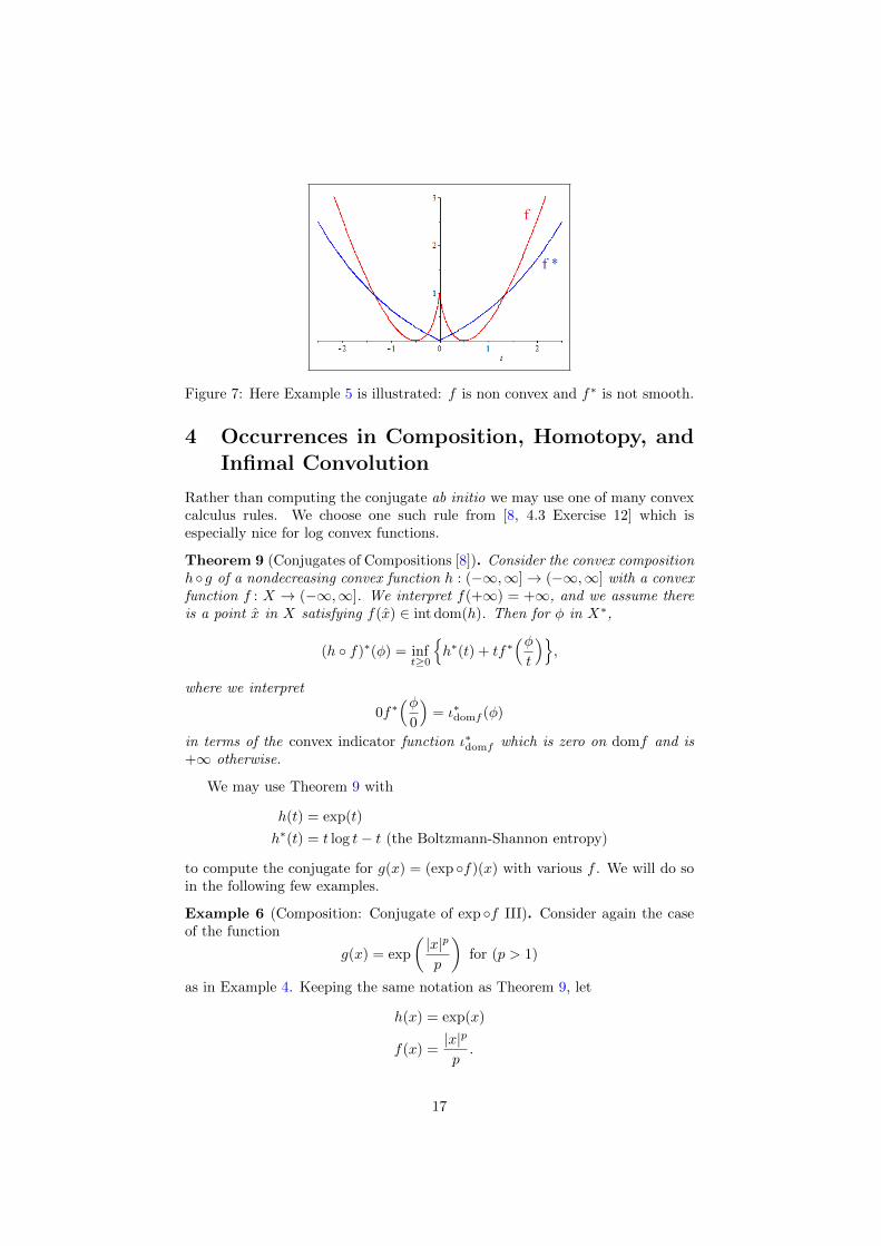
Figure 7: Here Example 5 is illustrated: f is non convex and f∗ is not smooth.

4 Occurrences in Composition, Homotopy, andInfimal Convolution

Rather than computing the conjugate ab initio we may use one of many convexcalculus rules. We choose one such rule from [8, 4.3 Exercise 12] which isespecially nice for log convex functions.

Theorem 9 (Conjugates of Compositions [8]). Consider the convex compositionh◦g of a nondecreasing convex function h : (−∞,∞]→ (−∞,∞] with a convexfunction f : X → (−∞,∞]. We interpret f(+∞) = +∞, and we assume thereis a point x in X satisfying f(x) ∈ int dom(h). Then for φ in X∗,

(h ◦ f)∗(φ) = inft≥0

{h∗(t) + tf∗

(φt

)},

where we interpret

0f∗(φ

0

)= ι∗domf (φ)

in terms of the convex indicator function ι∗domf which is zero on domf and is+∞ otherwise.

We may use Theorem 9 with

h(t) = exp(t)

h∗(t) = t log t− t (the Boltzmann-Shannon entropy)

to compute the conjugate for g(x) = (exp ◦f)(x) with various f . We will do soin the following few examples.

Example 6 (Composition: Conjugate of exp ◦f III). Consider again the caseof the function

g(x) = exp

(|x|p

p

)for (p > 1)

as in Example 4. Keeping the same notation as Theorem 9, let

h(x) = exp(x)

f(x) =|x|p

p.

17

Then we have that

h∗(x) = x log x− x (the Boltzmann-Shannon entropy)

f∗(x) =|x|q

qwhere

1

p+

1

q= 1.

Since g = h ◦ f , we may solve for g∗ by solving (h ◦ f)∗. From Theorem 9 wehave that, for φ 6= 0,

(h ◦ f)∗(φ) = inft≥0

{h∗(t) + tf∗

(φt

)}= inft≥0

{t log t− t+ t

(|φ|t

)q/q}.

Thus, if we can find a solution for t = s(p, φ) which minimizes

t log t− t+ t

(|φ|t

)q/q, (24)

we will be able to substitute s(p, y) for t and obtain a closed form for g∗, namely:

g∗(y) = s(p, y) ·(

log |s(p, y)| − 1 +1

q

(|φ|

s(p, y)

)q).

Differentiating Equation (24) with respect to t, setting the differentiated formequal to zero, and solving for t, we arrive at the optimal

t = s(p, y) = exp

(W ((q − 1)|y|q)

q

).

We may then substitute this value back into the objective function in Equa-tion (24) to obtain our closed form for g∗. The output from Maple appearsquite complicated, but this solution may be checked to be equivalent to thatexpressed in Equation (23). �

Any positively p-homogeneous convex function can be similarly treated.

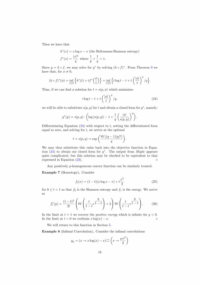
Example 7 (Homotopy). Consider

ft(x) = (1− t)(x log x− x) + tx2

2(25)

for 0 ≤ t < 1 so that f0 is the Shannon entropy and f1 is the energy. We arriveat

f∗t (y) =(1− t)2

2t

W t

1− te

y

1− t

+ 2

W t

1− te

y

1− t

. (26)

In the limit at t = 1 we recover the positive energy which is infinite for y < 0.In the limit at t = 0 we reobtain x log(x)− x. �

We will return to this function in Section 5.

Example 8 (Infimal Convolution). Consider the infimal convolutions

gµ = (x→ x log(x)− x)�

(x→ µx2

2

)

18

Figure 8: The convolution of entropy x log x − x and energy µx2/2 for µ =1/10, 10, and 100.

for µ > 0. This family is also called the Moreau envelope of x log(x)− x. Then,using the InfConv command in SCAT we arrive at

gµ(y) =µ

2y2 − 1

µW(µeµy)− 1

2µW(µeµy)2.

and gµ is fully explicit in terms of W. �

In Figure 8 we show how the infimal convolution produces a regularisationof everywhere finite approximations whose epigraphs converge back to that ofx log x−x as µ→ +∞. This is a special case of the Moreau-Yosida regularisationor resolvent [14].

Again each time W enters very naturally indeed.

5 Homotopy and entropy solution of inverse prob-lems

In [14, §4.7] we reprise the entropy solution of inverse problems. Consider the(negative) entropy functional1 defined as follows:

If : L1([0, 1], λ)→ R by

If (x) =

∫ 1

0

f(x(s)) ds

where λ is Lebesgue measure and f is a proper, closed convex function.

1We chose to solve convex minimization problems rather than maximizing the entropy.

19

Suppose we wish to minimize If subject to finitely many continuous linearconstraints of the form

〈ak, x〉 =

∫ 1

0

ak(s)x(s) ds = bk

for 1 ≤ k ≤ n. We may write this as

A : L1([0, 1])→ Rn by

Ax =

(∫ 1

0

a1(s)x(s) ds, . . . ,

∫ 1

0

an(s)x(s) ds

)= b.

Here necessarily ak ∈ L∞([0, 1], λ). When f∗ is smooth and everywhere finiteon the real line, our problem

infx∈L1

{If (x)|Ax = b} (27)

reduces to solving a finite nonlinear equation

∫ 1

0

(f∗)′

n∑j=1

λjaj(s)

ak(s) ds = bk (1 ≤ k ≤ n). (28)

The details of why all this is true are given in Section 7, and more informationcan be found in [9] including the matter of primal attainment and of constraintqualification.2 See also [13], [14, §4.7], [21], and [12, Theorem 6.3.4].

Let us consider a function ft of the form from Equation (25). If t = 1, thenf(x) = x2/2 and (f∗)′(x) = x and we are actually solving the classical Gramequations for a least square problem. If t = 0, then f is the Shannon Entropyand (f∗)′ = exp. Thus we restrict to considering cases where 0 < t < 1. Notethat Equation (28) relies only on (ft

∗)′. Most satisfactorily

(f∗t )′(y) =

(1− t)tW(

t

1− texp

(y

1− t

)). (29)

This is especially simple when t = 1/2 [8, p. 58]. As t tends to 0, we recover

limt→0

(f∗t )′(y) = exp(y)

as in the entropy case. Similarly, when t tends to 1, we obtain

limt→1

(f∗t )′(y) = max{y, 0}

which is the conjugate of the positive energy.

5.1 A general implementation

We illustrate by solving Equation (28) and Equation (29) for various values oft in the unit interval. We choose algebraic moments with ak(s) = sk−1 for

2When the moments are sufficiently analytic then feasibility assures the quasi-relative-interior CQ.

20

1 ≤ k ≤ 10 – though our methods work much more generally – and try toapproximate x(s) = 6

10 + sin(3πs2

)given the algebraic moments

bk =

∫ 1

0

x(s)a(s)ds =

∫ 1

0

(6

10+ sin

(3πs2

))· sk−1ds.

We do so by solving for λ ∈ Rn in the dual problem from Equation (28). Inother words, we wish to find the values λ1 . . . λ10 for which the subgradientvalues ∫ 1

0

(f∗t )′

n∑j=1

λjaj(s)

ak(s)ds− bk (30)

for k = 1..10 all evaluate to zero. By Equation (29), our subgradient (dualproblem) is represented more explicitly by the set of equations∫ 1

0

(1− t)tW

(t

1− texp

(∑nj=1 λjs

j−1

1− t

))sk−1ds− bk = 0. (31)

for k = 1 . . . 10. We can solve for λ using any standard numerical solver or, say,by a Newton-type method. We decide, largely for the sake of simplicity, to firstuse a classical Newton method. Indeed the Hessian computes nicely:

H(λ) = (hi,k)

hi,k =

∫ 1

0

(1− t)tW

(t

1− texp

(∑nj=1 λjaj(s)

1− t

))ak(s)ai(s)ds

=

∫ 1

0

(1− t)tW

(t

1− texp

(∑nj=1 λjs

j−1

1− t

))sk+i−2ds.

Our Hessian then turns out to be a Hankel matrix, greatly simplifying thecomputation. For each iteration, we need only to compute the 19 cases k + i =2 . . . 20 in order to fully populate our matrix. In fact, the gradient G(λ) may beobtained by taking the first row (or column) of the Hessian and subtracting bkfrom the kth entry. Thus, we need only to compute the Hessian and we obtainthe gradient for free. So in this case there is little extra work in using a secondorder method. In the case of trigonometric moments we similarly arrive at aToeplitz matrix.

5.2 Efficient computation of the dual

While there are reduced complexity methods for solving for λ as in Equation (30)with a Hankel matrix, they are less robust than more standard methods. In anyevent, it is advisable to solve Equation (30) without explicitly taking the inversebecause taking the inverse is significantly more computationally expensive forhigher order matrices.

The Newton direction is determined by solving

H(λn)(µ− λn) +G(λn) = 0 (32)

for µ and then setting λn+1 = λn + αn(µ − λn) for an appropriate step sizeαn > 0, which in the pure Newton method is αn = 1. See [1] and [2] for moregeneral options.

21

Since the actual computation of each of the 19 distinct Hessian terms requiresnumerical integration of the function

hi,k = h(i+k=α) =

∫ 1

0

(1− t)tW

(t

1− texp

(∑nj=1 λjs

j−1

1− t

))sαds,

where only the power α changes from one computation to the next, we canreduce the expense of computation quite easily.

Suppose we adopt a quadrature rule with weights {al}ml=1 and abcissas{xl}ml=1. Then, where

F (xl) =(1− t)tW

(t

1− texp

(∑nj=1 λjx

j−1l

1− t

)), (33)

for a single iteration of Newton’s method we need only use numerical integrationon the W function m times rather than order m · n times.

To see more clearly why this is the case, notice that we can reuse the valuesalF (xl), l = 1 . . .m as follows:

h1,1 =

m∑l=0

alF (xl)

h(i+k=α) =

m∑l=0

alF (xl)xα−2l .

Thus we need only compute each of them once for each iteration. We can alsostore each values xα−2l for l = 1 . . .m, α = 2 . . . 20 in a matrix at the beginning.

Our optimized process is then to take a fixed3 (Gaussian) quadrature ruleand to:

1. Precompute the weights {al}ml=1, and the abscissas raised to various powersxαl , l = 1 . . .m, α = 0 . . . 18, storing the weights in a vector and the powersof the abscissas in a matrix.

2. At each step compute the function values alF (xl), l = 1 . . .m, storingthem in a vector.

3. Compute the necessary 19 Hessian values∑ml=0 alF (xl)x

α−2l , α = 2 . . . 20.

If we properly create our matrix - of stored abscissa values raised to powers- we will be able to compute the Hessian values by simply multiplying ourvector from Step (2) by this matrix.

4. Use the resultant 19 values to build the Hessian and gradient and thensolve for the next iterate as in Equation (32).

The primal solution xt is then given in terms of the optimal multipliers in (31):

xt(s) =(1− t)tW

(t

1− texp

(∑nj=1 λjs

j−1

1− t

)). (34)

Note that this provides a functional form for the solution at all s in [0, 1], notonly for the quadrature points.

3We do not wish to allow automated decisions for adaptive methods without our control.

22

5.3 Some computed examples

The Maple code we used for computing the following examples is given in Ap-pendix 8. For the sake of consistency, all examples in this subsection werecomputed with 24 digits of precision, 20 abscissas, and a Newton step size of1/2. This reduced step dramatically improved convergence for t near 1. Whilethis precision is higher than would be used in production code, it allows us tosee the optimal performance of the algorithm.

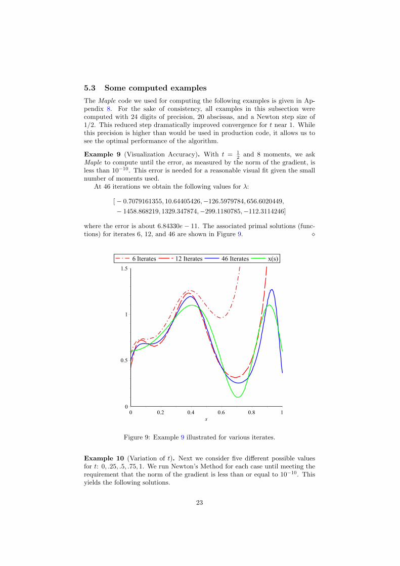
Example 9 (Visualization Accuracy). With t = 12 and 8 moments, we ask

Maple to compute until the error, as measured by the norm of the gradient, isless than 10−10. This error is needed for a reasonable visual fit given the smallnumber of moments used.

At 46 iterations we obtain the following values for λ:

[− 0.7079161355, 10.64405426,−126.5979784, 656.6020449,

− 1458.868219, 1329.347874,−299.1180785,−112.3114246]

where the error is about 6.84330e− 11. The associated primal solutions (func-tions) for iterates 6, 12, and 46 are shown in Figure 9. �

Figure 9: Example 9 illustrated for various iterates.

Example 10 (Variation of t). Next we consider five different possible valuesfor t: 0, .25, .5, .75, 1. We run Newton’s Method for each case until meeting therequirement that the norm of the gradient is less than or equal to 10−10. Thisyields the following solutions.

23

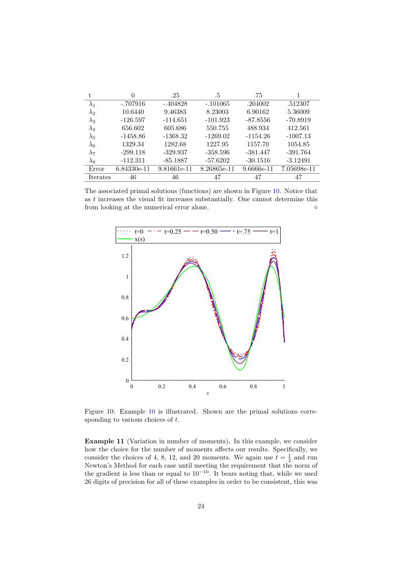
t 0 .25 .5 .75 1λ1 -.707916 -.404828 -.101065 .204002 .512307λ2 10.6440 9.46383 8.23003 6.90162 5.36009λ3 -126.597 -114.651 -101.923 -87.8556 -70.8919λ4 656.602 605.686 550.755 488.934 412.561λ5 -1458.86 -1368.32 -1269.02 -1154.26 -1007.13λ6 1329.34 1282.68 1227.95 1157.70 1054.85λ7 -299.118 -329.937 -358.596 -381.447 -391.764λ8 -112.311 -85.1887 -57.6202 -30.1516 -3.12491Error 6.84330e-11 9.81661e-11 8.26865e-11 9.6666e-11 7.05698e-11Iterates 46 46 47 47 47

The associated primal solutions (functions) are shown in Figure 10. Notice thatas t increases the visual fit increases substantially. One cannot determine thisfrom looking at the numerical error alone. �

Figure 10: Example 10 is illustrated. Shown are the primal solutions corre-sponding to various choices of t.

Example 11 (Variation in number of moments). In this example, we considerhow the choice for the number of moments affects our results. Specifically, weconsider the choices of 4, 8, 12, and 20 moments. We again use t = 1

2 and runNewton’s Method for each case until meeting the requirement that the norm ofthe gradient is less than or equal to 10−10. It bears noting that, while we used26 digits of precision for all of these examples in order to be consistent, this was

24

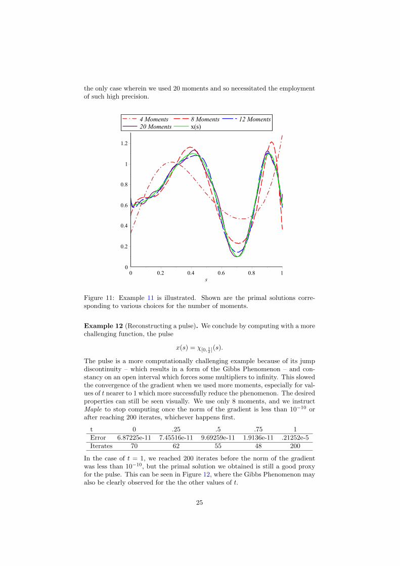
the only case wherein we used 20 moments and so necessitated the employmentof such high precision.

Figure 11: Example 11 is illustrated. Shown are the primal solutions corre-sponding to various choices for the number of moments.

Example 12 (Reconstructing a pulse). We conclude by computing with a morechallenging function, the pulse

x(s) = χ[0, 12 ](s).

The pulse is a more computationally challenging example because of its jumpdiscontinuity – which results in a form of the Gibbs Phenomenon – and con-stancy on an open interval which forces some multipliers to infinity. This slowedthe convergence of the gradient when we used more moments, especially for val-ues of t nearer to 1 which more successfully reduce the phenomenon. The desiredproperties can still be seen visually. We use only 8 moments, and we instructMaple to stop computing once the norm of the gradient is less than 10−10 orafter reaching 200 iterates, whichever happens first.

t 0 .25 .5 .75 1Error 6.87225e-11 7.45516e-11 9.69259e-11 1.9136e-11 .21252e-5Iterates 70 62 55 48 200

In the case of t = 1, we reached 200 iterates before the norm of the gradientwas less than 10−10, but the primal solution we obtained is still a good proxyfor the pulse. This can be seen in Figure 12, where the Gibbs Phenomenon mayalso be clearly observed for the the other values of t.

25

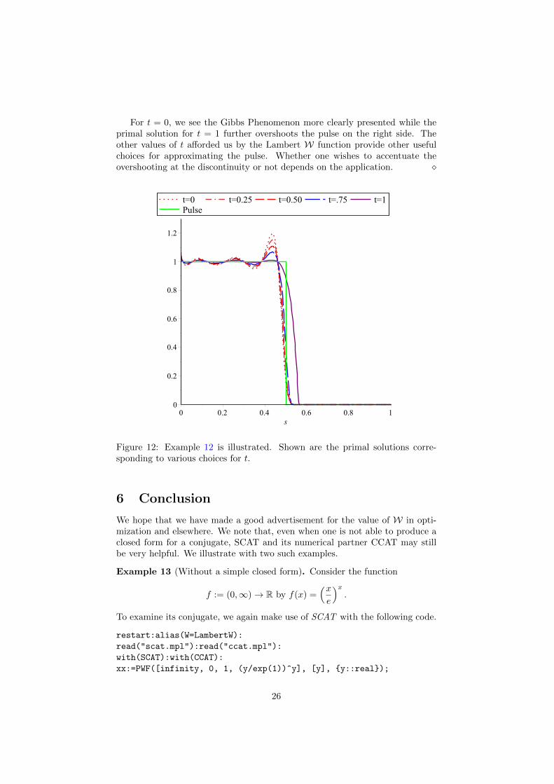
For t = 0, we see the Gibbs Phenomenon more clearly presented while theprimal solution for t = 1 further overshoots the pulse on the right side. Theother values of t afforded us by the Lambert W function provide other usefulchoices for approximating the pulse. Whether one wishes to accentuate theovershooting at the discontinuity or not depends on the application. �

Figure 12: Example 12 is illustrated. Shown are the primal solutions corre-sponding to various choices for t.

6 Conclusion

We hope that we have made a good advertisement for the value of W in opti-mization and elsewhere. We note that, even when one is not able to produce aclosed form for a conjugate, SCAT and its numerical partner CCAT may stillbe very helpful. We illustrate with two such examples.

Example 13 (Without a simple closed form). Consider the function

f := (0,∞)→ R by f(x) =(xe

)x.

To examine its conjugate, we again make use of SCAT with the following code.

restart:alias(W=LambertW):

read("scat.mpl"):read("ccat.mpl"):

with(SCAT):with(CCAT):

xx:=PWF([infinity, 0, 1, (y/exp(1))^y], [y], {y::real});

26

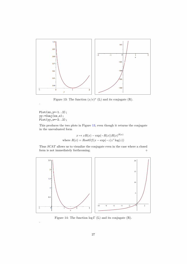
Figure 13: The function (x/e)x (L) and its conjugate (R)..

Plot(xx,y=-1..2);

yy:=Conj(xx,x);

Plot(yy,x=-2..2);

This produces the two plots in Figure 13, even though it returns the conjugatein the unevaluated form

x 7→ xR(x)− exp(−R(x))R(x)R(x)

where R(x) = RootOf(x− exp(−z)zz log(z))

Thus SCAT allows us to visualize the conjugate even in the case where a closedform is not immediately forthcoming. �

Figure 14: The function log Γ (L) and its conjugate (R)..

27

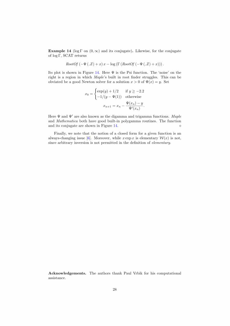
Example 14 (log Γ on (0,∞) and its conjugate). Likewise, for the conjugateof log Γ, SCAT returns

RootOf (−Ψ ( Z ) + x)x− log (Γ (RootOf (−Ψ ( Z ) + x))) .

Its plot is shown in Figure 14. Here Ψ is the Psi function. The ‘noise’ on theright is a region in which Maple’s built in root finder struggles. This can beobviated be a good Newton solver for a solution x > 0 of Ψ(x) = y. Set

x0 =

{exp(y) + 1/2 if y ≥ −2.2

−1/(y −Ψ(1)) otherwise

xn+1 = xn −Ψ(xn)− y

Ψ′(xn).

Here Ψ and Ψ′ are also known as the digamma and trigamma functions. Mapleand Mathematica both have good built-in polygamma routines. The functionand its conjugate are shown in Figure 14. �

Finally, we note that the notion of a closed form for a given function is analways-changing issue [6]. Moreover, while x expx is elementary W(x) is not,since arbitrary inversion is not permitted in the definition of elementary.

Acknowledgements. The authors thank Paul Vrbik for his computationalassistance.

28

References

[1] J. Barzilai and J.M. Borwein, “Two point step-size methods,” IMA Journalon Numerical Analysis, 8 (1988), 141–148.

[2] D. Bersetkas, “Projected newton methods for optimization problems withsimple constraints, ” SIAM. J. Control and Optimization 20(12) (1988),221–246.

[3] J.M. Borwein, “The SIAM 100 Digits Challenge,” Extended review for theMathematical Intelligencer, 27 (4) (2005), 40–48.

[4] J.M. Borwein and D.H. Bailey, Mathematics by Experiment: PlausibleReasoning in the 21st Century A.K. Peters Ltd, 2004. ISBN: 1-56881-136-5. Combined Interactive CD version 2006. Expanded Second Edition, 2008.

[5] J.M. Borwein, D.H. Bailey and R. Girgensohn, Experimentation in Math-ematics: Computational Paths to Discovery, A.K. Peters Ltd, 2004. ISBN:1-56881-211-6. Combined Interactive CD version 2006.

[6] J.M. Borwein and R.E. Crandall, “Closed forms: what they are and whywe care.” Notices Amer. Math. Soc. 60:1 (2013), 50–65.

[7] J.M. Borwein and C. Hamilton, “Symbolic convex analysis: algorithms andexamples,” Mathematical Programming, 116 (2009), 17–35.

[8] J.M. Borwein and A.S. Lewis, Convex Analysis and Nonlinear Optimiza-tion: Theory and Examples. Springer, (2000) (2nd Edition, 2006).

[9] J. M. Borwein and A. S. Lewis, “Duality relationships for entropy–likeminimization problems.” SIAM Control and Optim., 29 (1991), 325–338.

[10] J. M. Borwein, S. Reich, and S. Sabach, “A characterization of Bregmanfirmly nonexpansive operators using a new monotonicity concept,” Journalof Nonlinear and Convex Analysis. 12 (2011), 161–184.

[11] J. M. Borwein, A. Straub, J. Wan and W. Zudilin, with an Appendix byD. Zagier, “Densities of short uniform random walks.” Canadian. J. Math.64 (5), (2012), 961–990. Available at http://arxiv.org/abs/1103.2995.

[12] J.M. Borwein and J. D. Vanderwerff, Convex Functions : Constructions,Characterizations and Counterexamples. Cambridge University Press,(2010).

[13] J.M. Borwein and L. Yao, “Legendre-type integrands and convex integralfunctions,” Journal of Convex Analysis, 21 (2014), 264-288.

[14] J.M. Borwein and Q. Zhu, Techniques of Variational Analysis,CMS/Springer-Verlag, 2005. Paperback, 2010.

[15] S. Boyd and L. Vandenberghe, Convex Optimization, Cambridge UniversityPress. 2004.

[16] R.M. Corless, G.H. Gonnet, D.E.G. Hare, D.J. Jeffrey, and D.E. Knuth,“On the Lambert W function,” Advances in Computational Mathematics,5 (1996), 329-359.

29

[17] T.P. Dence, “A brief look into the Lambert W function,” Applied Mathe-matics, 4 (2013), 887-892.

[18] B. Fornberg and J.A.C. Weideman. “A numerical methodology for thePainleve equations.” Journal of Computational Physics, 230 (2011), 5957-5973.

[19] K.O. Geddes, M.L. Glasser, R.A. Moore, T.C. Scott. “Evaluation of classesof definite integrals involving elementary functions via differentiation ofspecial functions,” Applicable Algebra in Engineering, Communication andComputing, 1 (1990), 149-165.

[20] R.L. Graham, D.E. Knuth, O. Patashnik. Concrete Mathematics: A Foun-dation for Computer Science (2nd Edition). Addison-Wesley Professional.1994.

[21] D.E. Knuth, C.C. Rousseau, “A Stirling series: 10832,” American Math-ematical Monthly, 108 (2001), 877–878. http://dx.doi.org/10.2307/

2695574.

[22] S.B. Lindstrom Understanding the quasi relative interior. Project report onpermanent reserve at Portland State University Mathematics DepartmentLibary, (2015). http://docserver.carma.newcastle.edu.au/1682/.

[23] B.S. Mordukhovich and N.M. Nam, An Easy Path to Convex Analysis,Morgan & Claypool, 2014. ISBN: 9781627052375.

[24] M. Mrsevic. “Convexity of the inverse function,” The Teaching of Mathe-matics, XI (2008), 21-24.

[25] S.M. Stigler, “Stigler’s law of eponymy”. (F. Gieryn, ed.) ”Stigler’s law ofeponymy.” Transactions of the New York Academy of Sciences 39 (1980),147?58. doi:10.1111/j.2164-0947.1980.tb02775.x.

[26] Wikipedia contributors. “Lambert W function,” Wikipedia, The Free Ency-clopedia. https://en.wikipedia.org/w/index.php?title=Lambert_W_

function&oldid=716099641

[27] Wikipedia contributors. “Meijer G-function,” Wikipedia, The FreeEncyclopedia. https://en.wikipedia.org/w/index.php?title=Meijer_G-function&oldid=707287736

J.M. Borwein, CARMA, University of Newcastle, Callaghan, Australia, 2308E-mail address, J.M. Borwein: Jonathan.borwein@newcastle.edu.au

S.B. Lindstrom, CARMA, University of Newcastle, Callaghan, Australia, 2308E-mail address, S.B. Lindstrom: c3231022@uon.edu.au

30

7 Appendix on Conjugate duality

To see why solving Equation (27) reduces to solving Equation (28), we recallseveral results. We first recall from [14, Theorem 4.7.1] that:

Proposition 10. Suppose X is a Banach space, F : X → R ∪ {+∞} is alower semicontinuous convex function, A : X → Y is a linear operator, andb ∈ core(A domF ). Then

infx∈X{F (x)|Ax = b} = max

ϕ∈RN

{〈ϕ, b〉 − (F )∗(ATϕ)

}where AT denotes the adjoint map which satisfies

〈Au,ϕ〉Rn = 〈u,ATϕ〉L1 . (35)

This allows us to reformulate many primal problems as dual problems, mak-ing their solutions simpler to compute. In particular, the problem from Equa-tion (27) can be reformulated as

infx∈L1

{If (x)|Ax = b} = maxϕ∈RN

{〈ϕ, b〉 − (If )∗(ATϕ)

}. (36)

To the end of simplifying this further, we introduce another useful result. Werecall from [12, Theorem 6.3.4] that:

Proposition 11. If If is defined as above and f : R → (−∞,∞] is closed,proper, and convex, we have

(If )∗ = If∗ .

This allows us to express the dual problem more explicitly. In particular,since we have (If )∗ = If∗ , Equation (36) simplifies to

maxϕ∈RN

{〈ϕ, b〉 − If∗(ATϕ)

}= maxϕ∈RN

{〈ϕ, b〉 −

∫ 1

0

f∗(ATϕ)

}ds. (37)

Now in Equation (35), the inner product on the left is on Rn while the innerproduct on the right is the inner product on L1([0, 1]). Thus Equation (35)expands to

n∑k=1

(ϕk

∫ 1

0

ak(s)u(s) ds

)=

∫ 1

0

(ATϕ)u(s) ds.

This expansion should make it clear why we may simplify ATϕ further by writing

ATϕ =

n∑k=1

ϕkak(s).

Thus solving Equation (37) amounts to finding ϕ ∈ Rn which maximizes

n∑k=1

ϕkbk −∫ 1

0

f∗

(n∑k=1

ϕkak(s)

)ds. (38)

31

This is an equation which we can subdifferentiate. We maximize it by findingthe values of ϕk for which the subdifferential with respect to ϕ is zero. We firstrecall an equivalent characterisation for the convex subgradient. Recall thaty ∈ ∂F (x) if

〈y, z − x〉 ≤ F (z)− F (x) for all z ∈ X.For more preliminaries on subgradients, see, for Example, [23].

Lemma 12. For a convex function F , y is a subgradient of F at x if and onlyif

0 = F (x) + F ∗(y)− 〈y, x〉.

Proof. Taking the negative of both sides, we simply have

0 = −F (x) + 〈y, x〉 − supx∈X{〈y, x〉 − F (x)}.

Thus we have that

F (x)− 〈y, x〉 = − supx∈X{〈y, x〉 − F (x)} = inf

x∈X{F (x)− 〈y, x〉}

which is equivalent to

〈y, x− x〉 ≤ F (x)− F (x) for all x ∈ X.

This is the definition of the subgradient.

This makes it much easier for us to compute the subdifferential. In ourcontext, since (If )∗ = If∗ , we have from that Lemma 12 that y is a subgradientof If at x if and only if

0 = If (x) + If∗(y)− 〈y, x〉 =

∫f(x(s)) + f∗(y(s))− x(s)y(s) ds.

Now the integrand on the right is nonnegative by Fenchel-Young and so mustbe zero almost everywhere. However, Lemma 12 gives us that

f(x(s)) + f∗(y(s))− x(s)y(s) = 0 almost everywhere

if and only if y(s) is a subgradient of f at x(s) for almost all s. Thus we cansubdifferentiate with respect to each ϕk in Equation (38) and set equal to zero,obtaining n equations of the form

0 = bk −∫ 1

0

(f∗)′

n∑j=1

ϕjaj(s)

ak(s) ds.

Thus we have reduced the problem to that of solving Equation (28).

8 Appendix on Computation

8.1 Construction

We present the basic construction of the code in enough detail to reproduceExample 9 and using the corresponding Initialization values. It is straightfor-ward to adapt the basic code to reproduce the other examples. We elect, for

32

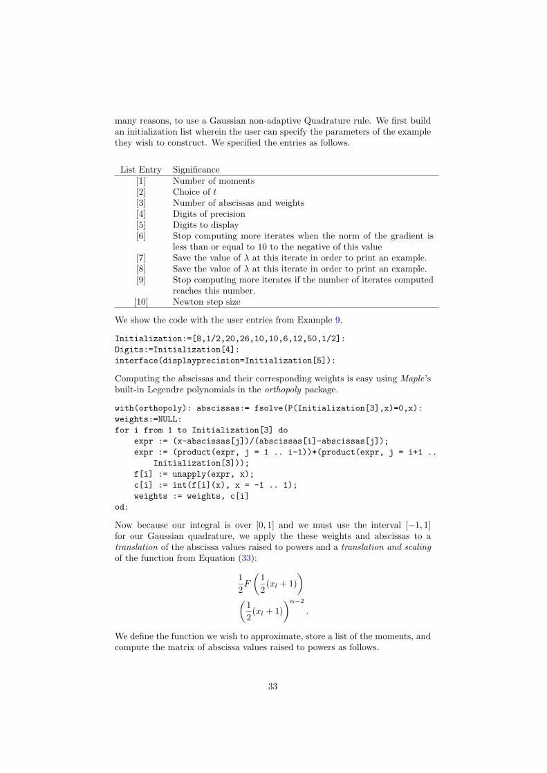
many reasons, to use a Gaussian non-adaptive Quadrature rule. We first buildan initialization list wherein the user can specify the parameters of the examplethey wish to construct. We specified the entries as follows.

List Entry Significance[1] Number of moments[2] Choice of t[3] Number of abscissas and weights[4] Digits of precision[5] Digits to display[6] Stop computing more iterates when the norm of the gradient is

less than or equal to 10 to the negative of this value[7] Save the value of λ at this iterate in order to print an example.[8] Save the value of λ at this iterate in order to print an example.[9] Stop computing more iterates if the number of iterates computed

reaches this number.[10] Newton step size

We show the code with the user entries from Example 9.

Initialization:=[8,1/2,20,26,10,10,6,12,50,1/2]:

Digits:=Initialization[4]:

interface(displayprecision=Initialization[5]):

Computing the abscissas and their corresponding weights is easy using Maple’sbuilt-in Legendre polynomials in the orthopoly package.

with(orthopoly): abscissas:= fsolve(P(Initialization[3],x)=0,x):

weights:=NULL:

for i from 1 to Initialization[3] do

expr := (x-abscissas[j])/(abscissas[i]-abscissas[j]);

expr := (product(expr, j = 1 .. i-1))*(product(expr, j = i+1 ..

Initialization[3]));

f[i] := unapply(expr, x);

c[i] := int(f[i](x), x = -1 .. 1);

weights := weights, c[i]

od:

Now because our integral is over [0, 1] and we must use the interval [−1, 1]for our Gaussian quadrature, we apply the these weights and abscissas to atranslation of the abscissa values raised to powers and a translation and scalingof the function from Equation (33):

1

2F

(1

2(xl + 1)

)(

1

2(xl + 1)

)α−2.

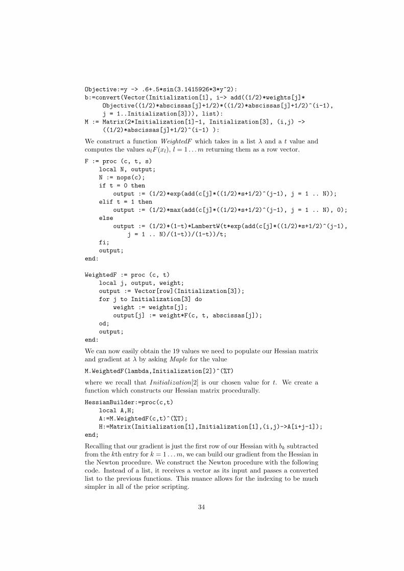
We define the function we wish to approximate, store a list of the moments, andcompute the matrix of abscissa values raised to powers as follows.

33

Objective:=y -> .6+.5*sin(3.1415926*3*y^2):

b:=convert(Vector(Initialization[1], i-> add((1/2)*weights[j]*

Objective((1/2)*abscissas[j]+1/2)*((1/2)*abscissas[j]+1/2)^(i-1),

j = 1..Initialization[3])), list):

M := Matrix(2*Initialization[1]-1, Initialization[3], (i,j) ->

((1/2)*abscissas[j]+1/2)^(i-1) ):

We construct a function WeightedF which takes in a list λ and a t value andcomputes the values alF (xl), l = 1 . . .m returning them as a row vector.

F := proc (c, t, s)

local N, output;

N := nops(c);

if t = 0 then

output := (1/2)*exp(add(c[j]*((1/2)*s+1/2)^(j-1), j = 1 .. N));

elif t = 1 then

output := (1/2)*max(add(c[j]*((1/2)*s+1/2)^(j-1), j = 1 .. N), 0);

else

output := (1/2)*(1-t)*LambertW(t*exp(add(c[j]*((1/2)*s+1/2)^(j-1),

j = 1 .. N)/(1-t))/(1-t))/t;

fi;

output;

end:

WeightedF := proc (c, t)

local j, output, weight;

output := Vector[row](Initialization[3]);

for j to Initialization[3] do

weight := weights[j];

output[j] := weight*F(c, t, abscissas[j]);

od;

output;

end:

We can now easily obtain the 19 values we need to populate our Hessian matrixand gradient at λ by asking Maple for the value

M.WeightedF(lambda,Initialization[2])^(%T)

where we recall that Initialization[2] is our chosen value for t. We create afunction which constructs our Hessian matrix procedurally.

HessianBuilder:=proc(c,t)

local A,H;

A:=M.WeightedF(c,t)^(%T);

H:=Matrix(Initialization[1],Initialization[1],(i,j)->A[i+j-1]);

end;

Recalling that our gradient is just the first row of our Hessian with bk subtractedfrom the kth entry for k = 1 . . .m, we can build our gradient from the Hessian inthe Newton procedure. We construct the Newton procedure with the followingcode. Instead of a list, it receives a vector as its input and passes a convertedlist to the previous functions. This nuance allows for the indexing to be muchsimpler in all of the prior scripting.

34

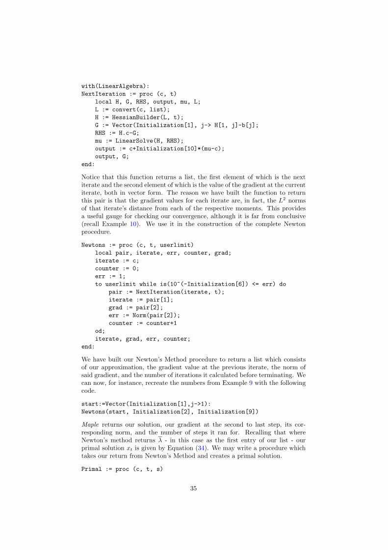
with(LinearAlgebra):

NextIteration := proc (c, t)

local H, G, RHS, output, mu, L;

L := convert(c, list);

H := HessianBuilder(L, t);

G := Vector(Initialization[1], j-> H[1, j]-b[j];

RHS := H.c-G;

mu := LinearSolve(H, RHS);

output := c+Initialization[10]*(mu-c);

output, G;

end:

Notice that this function returns a list, the first element of which is the nextiterate and the second element of which is the value of the gradient at the currentiterate, both in vector form. The reason we have built the function to returnthis pair is that the gradient values for each iterate are, in fact, the L2 normsof that iterate’s distance from each of the respective moments. This providesa useful gauge for checking our convergence, although it is far from conclusive(recall Example 10). We use it in the construction of the complete Newtonprocedure.

Newtons := proc (c, t, userlimit)

local pair, iterate, err, counter, grad;

iterate := c;

counter := 0;

err := 1;

to userlimit while is(10^(-Initialization[6]) <= err) do

pair := NextIteration(iterate, t);

iterate := pair[1];

grad := pair[2];

err := Norm(pair[2]);

counter := counter+1

od;

iterate, grad, err, counter;

end:

We have built our Newton’s Method procedure to return a list which consistsof our approximation, the gradient value at the previous iterate, the norm ofsaid gradient, and the number of iterations it calculated before terminating. Wecan now, for instance, recreate the numbers from Example 9 with the followingcode.

start:=Vector(Initialization[1],j->1):

Newtons(start, Initialization[2], Initialization[9])

Maple returns our solution, our gradient at the second to last step, its cor-responding norm, and the number of steps it ran for. Recalling that whereNewton’s method returns λ - in this case as the first entry of our list - ourprimal solution xt is given by Equation (34). We may write a procedure whichtakes our return from Newton’s Method and creates a primal solution.

Primal := proc (c, t, s)

35

local sumterm, L, output;

L := convert(c, list);

sumterm := add(L[j]*s^(j-1), j = 1 .. Initialization[1]);

if t = 0 then

output := exp(sumterm);

elif t = 1 then

output := max(sumterm, 0);

else

output := (1-t)*LambertW(t*exp(sumterm/(1-t))/(1-t))/t

fi;

output;

end:

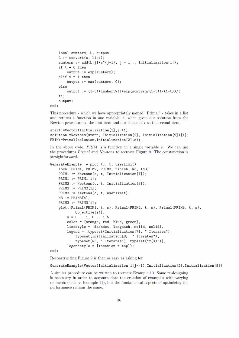
This procedure - which we have appropriately named ”Primal” - takes in a listand returns a function in one variable, s, when given our solution from theNewton procedure as the first item and our choice of t as the second item.

start:=Vector(Initialization[1],j->1):

solution:=Newtons(start, Initialization[2], Initialization[9])[1];

PRIM:=Primal(solution,Initialization[2],s);

In the above code, PRIM is a function in a single variable s. We can usethe procedures Primal and Newtons to recreate Figure 9. The construction isstraightforward.

GenerateExample := proc (c, t, userlimit)

local PRIM1, PRIM2, PRIM3, finish, N3, IMG;

PRIM1 := Newtons(c, t, Initialization[7]);

PRIM1 := PRIM1[1];

PRIM2 := Newtons(c, t, Initialization[8]);

PRIM2 := PRIM2[1];

PRIM3 := Newtons(c, t, userlimit);

N3 := PRIM3[4];

PRIM3 := PRIM3[1];

plot([Primal(PRIM1, t, s), Primal(PRIM2, t, s), Primal(PRIM3, t, s),

Objective(s)],

s = 0 .. 1, 0 .. 1.5,

color = [orange, red, blue, green],

linestyle = [dashdot, longdash, solid, solid],

legend = [typeset(Initialization[7], " Iterates"),

typeset(Initialization[8], " Iterates"),

typeset(N3, " Iterates"), typeset("x(s)")],

legendstyle = [location = top]);

end:

Reconstructing Figure 9 is then as easy as asking for

GenerateExample(Vector(Initialization[1]j->1),Initialization[2],Initialization[9])

A similar procedure can be written to recreate Example 10. Some re-designingis necessary in order to accommodate the creation of examples with varyingmoments (such as Example 11), but the fundamental aspects of optimizing theperformance remain the same.

36