Embed Size (px)
Citation preview
Medium-term morphodynamics of the Mittelplate area, German
North Sea coast
Dissertation zur Erlangung des Doktorgrades
der Mathematisch-Naturwissenschaftlichen Fakultät der Christian-Albrechts-Universität zu Kiel
vorgelegt von Thi Thuy Diem Nguyen
Kiel, 2015

Erste Gutacher: Prof. Dr. Roberto Mayerle
Zweite Gutachter: Prof. Dr. Athanasios Vafeidis
Tag der mündlichen Prüfung: 24.11.2015
Zum Druck genehmigt: 24.11.2015
gez. Prof. Dr. Wolfgang J. Duschl, Dekan
“Gedruckt mit Unterstützung des Deutschen Akademischen Austauschdienstes“


Acknowledgements
First of all, I would like to express my deepest gratitude to my supervisor, Prof. Dr. Roberto Mayerle, for his excellent guidance, support and encouragement. I sincerely thank him for his valuable comments and advice which kept me on the right track throughout my PhD study. I would also like to thank Prof. Dr. Athanasios Vafeidis for being the second referee of my thesis.
I would like to thank Dr. Karl-Heinz Runte for sharing his knowledge and providing constructive comments and suggestions for the improvement of my thesis. I also thank him for translating the thesis abstract to German.
I acknowledge the German Academic Exchange Service (Deutsche Akademische Austauschdienst - DAAD) for the financial support.
My gratitude is extended to Dr. Rangaswami Narayanan for helpful discussions and for editing my thesis at the early stage. Many thanks to Dr. Talal Etri for discussions on modelling issues. I would like to thank Dr. Peter Weppen for his kind help with administration tasks and encouragement during my study.
My thanks also go to the colleagues at the Coastal Research Laboratory for their friendship and a nice working atmosphere.
Lastly, I am grateful to my parents and my sister for continuous support and encouragement. Special thanks go to my husband, Dr. Quang Dung Lam, for being supportive and understanding. I am especially thankful to my daughter, Thu Ha, and my son, Quang Minh, for bringing so much joy into my life and inspiring me to finish this thesis.
Thi Thuy Diem Nguyen
i

ii
Abstract In view of climate change and sea level rise the prediction of the morphological evolution of coastal areas in medium-term and long-term has become a matter of increasing concern in the field of coastal management. Process-based modelling has recently emerged as an effective tool for studying coastal morphodynamics and for predictive estimation of the coastal development.
The main focus of the thesis is to study, analyse and assess the medium-term morphodynamics of a complex network of tidal channels, flats and shoals in the Mittelplate area, Dithmarschen Bight, German North Sea coast. In this framework numerical techniques for accelerating morphodynamic simulations are also critically evaluated.
Taking full advantage of recent available high-resolution bathymetric surveys over a period of six years, the natural morphodynamics was thoroughly investigated. Essential reasons for the morphological changes are provided on the base of a structural analysis. The medium-term morphological changes were studied by means of numerical modelling. Process-based models for simulating flow, waves and sediment transport were developed, calibrated and validated against collected field data. According to internationally accepted quality criteria the developed models proved to represent well the hydrodynamics and sediment dynamics in the area of concern. By means of coupling of the process models a morphodynamic model was set-up.
Benchmark simulation using the full time series of forcing of tide, wind and waves was conducted for a two-year period and the model proved good ability in reproducing the observed morphological changes. The single effects of the driving forces tide, wind and waves on the morphological development were analyzed and assessed. Main mechanisms driving the morphological evolution of the area were identified.
An input reduction method, the so-called "representative period method" applied to time series of wind in conjunction with "morphological factor approach", was used to analyse effectiveness of numerically accelerated simulations for the prediction of morphodynamics. The results show that the method was restrictively applicable for reproducing the medium-term morphodynamics because (i) it disregards associated classes of wind speed and wind direction in time series when shortening the long-term wind data to much shorter "representative period" data; (ii) the interaction of tide, wind and waves from long-term is changed or widely lost in the "representative period". Recommendations for the improvement of the applied input reduction method and the model performance are provided.
iii

iv
Zusammenfassung Im Angesicht von Klimawandel und Meeresspiegelanstieg ist die Vorhersage der mittel- und langfristigen morphologischen Entwicklung von Küstengebieten von steigendem Interesse im Küstenmanagement. Hier sind prozessbasierte numerische Modelle zu effizienten Werkzeugen für Studien zur Morphodynamik und für vorausblickende Abschätzungen der Küstenentwicklung geworden.
Hauptziel der Arbeit ist die Untersuchung, Analyse und Einschätzung der mittelfristigen Morphodynamik in einem komplexen System aus Gezeitenrinnen, Wattflächen und Wattrücken im Mittelplate-Gebiet der Dithmarscher Bucht, Deutsche Nordseeküste. Dabei werden auch numerische Techniken zur Beschleunigung morphodynamischer Simulationen kritisch beleuchtet.
Unter Verwendung vorliegender hochauflösender topografischer Vermessungen über einen Zeitraum von 6 Jahren wird zunächst die natürliche Morphodynamik betrachtet. Über Strukturanalysen werden wesentliche Gründe für morphologische Veränderungen offengelegt. Mit Hilfe numerischer Modellierungen werden dann die mittelfristigen morphologischen Veränderungen eingehender untersucht. Dazu wurden prozessbasierte Modelle zur Simulation von Strömung, Seegang und Sedimenttransport entwickelt, kalibriert und verifiziert. Gemäß internationalen Prüfverfahren sind die Modelle befähigt, Hydro- und Schwebstoffdynamik im Zielgebiet in guter Qualität zu reproduzieren. Durch Kopplung der prozessbasierten Modelle wurde ein Morphodynamikmodell aufgebaut.
Eine „Benchmark“-Simulation mit vollständiger Zeitreihe der Antriebsgrößen Tide, Wind und Seegang wurde für einen Zeitraum von 2 Jahren durchgeführt. Eine Gegenüberstellung mit Topografiedaten unterstrich die Fähigkeit dieses Modells, die beobachtete Morphologieentwicklung gut zu reproduzieren. Mit dem Modell wurden die Einzeleffekte der Antriebsgrößen auf die morphologische Entwicklung analysiert, bewertet und die Hauptantriebsmechanismen identifiziert.
Das Eingabereduktionsverfahren „Repräsentative Periode Methode“, wurde für Windzeitreihen angewandt und mit dem Ansatz „Morphologischer Faktor“ kombiniert, um die Effizienz numerisch beschleunigter Simulationen zur Vorhersage der Morphodynamik zu analysieren. Es wird gezeigt, dass diese Verfahren zur Reproduktion der mittelfristigen Morphodynamik eher eingeschränkt anzuwenden sind, weil a) sie eine Zusammengehörigkeit von Gruppen von Windgeschwindigkeit und Windrichtung bei der numerischen Zerschneidung der Langzeitreihen zu weit kürzeren „repräsentativen Perioden“ außer Acht lassen, und weil b) die Interaktion von Zeitreihengruppen aus Tide, Wind und Seegang durch Verkürzung zu „repräsentativen Perioden“ geändert werden oder verloren gehen. Es werden Empfehlungen zur Verbesserung der angewandten Reduktionstechnik und der Modellleistung gegeben
v

vi

List of Symbols
Symbol Units Meaning
a [m] reference height for suspended sediment concentration
C [m1/2/s] Chezy coefficient
c [kg/m3] mass sediment concentration
ca [kg/m3] mass sediment concentration at reference height a
d50 [µm] median grain diameter
fMOR [-] morphological scale factor
g [m/s2] gravity acceleration
Hs [m] significant wave height
M [kg m-2s-1] erosion parameter
uE [m/s] eastward current velocity
uN [m/s] northward current velocity
ws [mm/s] fall velocity
∆t [s] flow time step
η [m] water level above reference level
ρa [kg/m3] air density
ρs [kg/m3] sediment density
vii

List of Symbols
ρw [kg/m3] water density
ν [m2/s] horizontal viscosity
τcr,e [N/m2] critical shear stress for erosion
τcr,d [N/m2] critical shear stress for deposition
τcw [N/m2] maximum shear stress due to waves and current
viii
Contents
Acknowledgements .................................................................................................i
Abstract................................................................................................................. iii
Zusammenfassung .................................................................................................v
List of Symbols .................................................................................................... vii
Contents .................................................................................................................ix
List of Figures..................................................................................................... xiii
List of Tables .......................................................................................................xxi
Chapter 1 Introduction .......................................................................................1
1.1 General introduction ....................................................................................1
1.2 Aim and objectives ......................................................................................2
1.3 Outline of the thesis .....................................................................................4
Chapter 2 Literature review ................................................................................5
2.1 Introduction..................................................................................................5
2.2 Approaches to morphodynamic modelling..................................................7
2.2.1 Model reduction.......................................................................................7
2.2.2 Input reduction.........................................................................................9
2.3 Representative period method ...................................................................10
2.4 Process-based morphodynamic models .....................................................11
2.5 Delft3D model ...........................................................................................13
2.5.1 Hydrodynamic model ............................................................................13
ix
Contents
2.5.2 Wave model ...........................................................................................15
2.5.3 Sediment transport model ......................................................................16
2.5.4 Morphodynamic model..........................................................................18
2.6 Model nesting ............................................................................................20
2.7 Meteorological models ..............................................................................21
2.8 Statistical parameters for evaluation of model performance .....................21
2.8.1 Statistical parameters in hydrodynamic modelling................................21
2.8.2 Statistical parameters in sediment transport modelling .........................23
2.8.3 Statistical parameters in morphodynamic modelling.............................23
Chapter 3 Study area and available data ........................................................25
3.1 Introduction................................................................................................25
3.2 Hydrodynamic processes ...........................................................................26
3.2.1 Tidal conditions .....................................................................................26
3.2.2 Wave conditions ....................................................................................27
3.3 Meteorological conditions .........................................................................29
3.4 Storm surges ..............................................................................................32
3.5 Salinity and water temperature ..................................................................32
3.6 Geological feature and sediment characteristics........................................33
3.6.1 Geological feature..................................................................................33
3.6.2 Seabed surface sediments ......................................................................36
3.6.3 Suspended sediments .............................................................................36
3.7 Morphology and morphodynamics............................................................36
3.8 Coastal processes measurements ...............................................................37
3.8.1 Measuring of current velocity................................................................37
3.8.2 Measuring of suspended load ................................................................40
3.9 Data used in the study................................................................................42
3.9.1 Meteorological data ...............................................................................42
3.9.2 Hydrodynamic and sediment dynamic data...........................................42
3.9.3 Bathymetric data ....................................................................................43
x
Contents
Chapter 4 Medium-term morphodynamic evolution of the Mittelplate area - field measurements............................................................................................47
4.1 Introduction................................................................................................47
4.2 Methods .....................................................................................................47
4.3 Results........................................................................................................49
4.3.1 Changes of the selected morphological elements ..................................49
4.3.2 Changes of depth contour ......................................................................54
4.3.3 Changes of channel cross-sections ........................................................55
4.4 Discussion..................................................................................................62
Chapter 5 The Mittelplate models....................................................................65
5.1 Introduction................................................................................................65
5.1.1 Model domain ........................................................................................65
5.1.2 Model grids ............................................................................................66
5.1.3 Model bathymetry..................................................................................67
5.2 Flow model ................................................................................................68
5.2.1 Flow model setup...................................................................................69
5.2.2 Flow model sensitivity analysis and calibration ....................................70
5.2.3 Flow model validation ...........................................................................80
5.3 Wave model ...............................................................................................87
5.3.1 Wave model set up.................................................................................87
5.3.2 Wave model sensitivity analysis and calibration...................................87
5.3.3 Wave model validation ..........................................................................90
5.4 Sediment transport model ..........................................................................91
5.4.1 Sediment transport model set up............................................................91
5.4.2 Sediment transport model sensitivity and calibration............................92
5.4.3 Sediment transport model validation ...................................................100
5.5 Morphodynamic model............................................................................104
5.6 Discussion................................................................................................106
xi
Contents
Chapter 6 Medium-term morphodynamic evolution of the Mittelplate area - numerical modelling........................................................................................109
6.1 Introduction..............................................................................................109
6.2 Methods ...................................................................................................110
6.2.1 Benchmark simulations........................................................................111
6.2.2 Accelerated simulations.......................................................................112
6.2.3 Selection of representative periods ......................................................113
6.3 Environmental conditions ........................................................................114
6.3.1 Environmental condition during the two-year period 2006-2008 .......114
6.3.2 Environmental condition during the selected representative periods ..115
6.4 Results......................................................................................................119
6.4.1 Benchmark simulations........................................................................119
6.4.2 Effect of tide on the medium-term morphodynamics ..........................127
6.4.3 Effect of wind on the medium-term morphodynamics ........................129
6.4.4 Effect of waves on the medium-term morphodynamics ......................131
6.4.5 Input reduction method - tide only case...............................................132
6.4.6 Input reduction method - tide and wind forcing case ..........................138
6.4.7 Input reduction method - all forcing case ............................................145
6.5 Discussion................................................................................................152
6.5.1 Performance of the benchmark morphodynamic model......................152
6.5.2 Driving forces and mechanisms of channel migration ........................154
6.5.3 Performance of the accelerated morphodynamic models ....................155
Chapter 7 Conclusions and recommendations..............................................163
7.1 Conclusions..............................................................................................164
7.2 Recommendations....................................................................................167
References...........................................................................................................169
Erklärung ...........................................................................................................175
xii
List of Figures
Figure 1.1. Location of the study area in the Dithmarschen Bight, North Sea........3
Figure 2.1. Spatial and temporal scales (after Cowell and Thom, 1994) ................6
Figure 2.2. Flow diagram of online morphodynamic model setup (Roelvink, 2006) ................................................................................................................8
Figure 2.3. Staggered grid of Delft3D-FLOW (Deltares, 2008a)..........................14
Figure 2.4. Continental Shelf Model and German Bight Model ...........................20
Figure 3.1. Channel system of the Mittelplate area ...............................................26
Figure 3.2. Classification of tidal areas according to Hayes (1979) for mean tidal range and mean wave height. The western and eastern parts of the Dithmarschen Bight are indicated by the dark and light grey boxes, respectively (Wilkens, 2004) .........................................................................27
Figure 3.3. Location of wave measurements .........................................................28
Figure 3.4. Measured significant wave heights from 27 April to 19 August 2009 at two stations W1 and W2 ...................................................................28
Figure 3.5. Measured water levels and significant wave heights at station W1 ....29
Figure 3.6. Wind rose at the Dithmarschen Bight for the period 1989-2000 based on PRISMA data (Wilkens, 2004).......................................................30
Figure 3.7. Wind rose at the Dithmarschen Bight for the period 2000-2008 based on DWD data .......................................................................................30
Figure 3.8. Wind roses of 12 months at the Dithmarschen Bight in the period 2000-2008 based on DWD data.....................................................................31
xiii
List of Figures
Figure 3.9. Salinity and temperature patterns a long cross-section C4 on 06 October 2009..................................................................................................33
Figure 3.10. Thickness of the potentially mobile sediment layer in the Central Dithmarschen Bight (Asp, 2004) ......................................................34
Figure 3.11. Schematic representation of the Holocene sedimentary sequences (after Dittmer, 1938).....................................................................34
Figure 3.12. Sedimentary stratification from sediment cores around the oil platform in 2008.............................................................................................35
Figure 3.13. Measuring technique along a transect (after Poerbandono and Mayerle, 2005)...............................................................................................37
Figure 3.14. ADCP beam pattern (Simpson, 2001)...............................................38
Figure 3.15. Example of raw ADCP north (upper) and east (lower) velocities along a transect measured from a moving vessel ..........................................39
Figure 3.16. Example of raw north (left) and east (right) velocity profiles measured from a moving vessel.....................................................................39
Figure 3.17. Sampler mounted with CTD sensors and optical beam transmissometer .............................................................................................41
Figure 3.18. Example of a calibration curve. Optical transmission is related to sediment concentration ..............................................................................41
Figure 3.19. Measurement locations and transects for hydrodynamic and sediment dynamic data...................................................................................43
Figure 4.1. Location of the morphological elements Trischenflinge, TF, S1, S2, CN2, CN3 and of the cross-sections W, MP, E selected for the analysis of natural medium-term evolution of the Mittelplate area (measured bathymetry in 2008) .....................................................................48
Figure 4.2. Yearly measured bathymetries from 2006-2012 .................................51
Figure 4.3. Yearly measured bathymetry differences. Bathymetric contour in the former year...............................................................................................53
Figure 4.4. Changes of -2 mNN depth contour of the channel system..................54
Figure 4.5. Measured morphological changes at cross-section W ........................56
Figure 4.6. Migration rates of the two channel banks at -4 mNN depth contour at cross-section W.............................................................................56
xiv
List of Figures
Figure 4.7. Changes of the cross-sectional area below the -4 mNN depth contour at cross-section W.............................................................................57
Figure 4.8. Migration rates at the -4 mNN depth contour vs. cross-sectional area below the -4 mNN level at cross-section W...........................................57
Figure 4.9. Measured morphological changes at cross-section MP ......................58
Figure 4.10. Changes of the cross-sectional area below the -4 mNN depth contour at cross-section MP...........................................................................59
Figure 4.11. Measured morphological changes at cross-section E........................60
Figure 4.12. Migration rates of the two channel banks at the -4 mNN depth contour at cross-section E ..............................................................................60
Figure 4.13. Changes of the cross-sectional area below -4 mNN depth contour at the cross-section E ........................................................................61
Figure 4.14. Migration rates at the -4 mNN depth contour vs. cross-sectional area below the -4 mNN depth contour at cross-section E..............................61
Figure 5.1. Model domain of the Mittelplate area. Bathymetry is combined from measured data in the years 1999, 2002, 2005 and 2006 .......................66
Figure 5.2. Flow grid of the Mittelplate model......................................................67
Figure 5.3. Flow grid and bathymetry (in 2008) in the area of interest of the Mittelplate model...........................................................................................68
Figure 5.4. Nesting sequence for the generation of the open boundary conditions of the Mittelplate Model...............................................................69
Figure 5.5. Location of the monitoring point selected for the sensitivity analysis of the flow model .............................................................................70
Figure 5.6. Sensitivity of boundary conditions to computed water levels and current velocities............................................................................................71
Figure 5.7. Sensitivity of bottom roughness to computed water levels and current velocities............................................................................................72
Figure 5.8. Sensitivity of eddy viscosity to computed water levels and current velocities............................................................................................73
Figure 5.9. Comparisons of computed and measured water levels at gauge stations Büsum, Flackstrom and Mittelplate in the calibration period ..........75
xv
List of Figures
Figure 5.10. RMAE of the computed velocities with different bottom roughness parameters.....................................................................................76
Figure 5.11. Measured vs. computed variation of cross-sectional distribution of eastward uE and northward uN current velocities at cross-section C1 on 05 September 2007 ...................................................................................77
Figure 5.12. Comparison of measured and computed depth-averaged current velocity patterns at cross-section C2s on 20 February 2007 .........................78
Figure 5.13. Comparison of measured and computed cross-sectional eastward uE and northward uN current velocities at cross-section C2s on 20 February 2007 ...........................................................................................78
Figure 5.14. Comparison of measured and computed depth-averaged current velocity patterns at cross-section C3 on 01 July 2009...................................79
Figure 5.15. Comparison of measured and computed cross-sectional eastward uE and northward uN current velocities at cross-section C3 on 01 July 2009...................................................................................................79
Figure 5.16. Comparison of measured and computed cross-sectional eastward uE and northward uN current velocities at cross-section C4 on 28 April 2009 .................................................................................................80
Figure 5.17. Comparisons of water levels at gauge stations Büsum, Flackstrom and Mittelplate in the validation period......................................81
Figure 5.18. Comparison of measured and computed depth-averaged current velocity patterns at cross-section C1 on 23 November 2006.........................83
Figure 5.19. Comparison of measured and computed cross-sectional eastward (uE) and northward (uN) current velocities at cross-section C1 on 23 November 2006....................................................................................83
Figure 5.20. Comparison of measured and computed depth-averaged current velocity patterns at cross-section C2l on 23 November 2006 .......................84
Figure 5.21. Comparison of measured and computed cross-sectional eastward (uE) and northward (uN) current velocities at cross-section C2l on 23 November 2006....................................................................................84
Figure 5.22. Comparison of measured and computed depth-averaged current velocity patterns at cross-section C3 on 17 (left) and 18 (right) September 2009 .............................................................................................85
xvi
List of Figures
Figure 5.23. Comparison of measured and computed cross-sectional eastward (uE) and northward (uN) current velocities at cross-section C3 on 17 and 18 September 2009........................................................................85
Figure 5.24. Comparison of measured and computed depth-averaged current velocity patterns at cross-section C4 on 17 June 2009 ..................................86
Figure 5.25. Comparison of measured and computed cross-sectional eastward (uE) and northward (uN) current velocities at cross-section C4 on 17 June 2009 .............................................................................................86
Figure 5.26. Sensitivity of wave grid to significant wave heights.........................88
Figure 5.27. RMAE (upper) and r (lower) of computed significant wave heights with different coupling intervals between flow and wave modules..........................................................................................................89
Figure 5.28. Comparisons of modelled and measured significant wave heights at the stations W1 and W2 in the calibration period .........................90
Figure 5.29. Comparisons of modelled and measured significant wave heights at stations W1 and W2 in the validation period ................................91
Figure 5.30. Cross-sections and stations of measured sediment concentration.....93
Figure 5.31. Sensitivity of wave effect to sediment concentration........................96
Figure 5.32. Sensitivity of sediment grain size to sediment concentration ...........96
Figure 5.33. Sensitivity of critical shear stress for erosion to sediment concentration..................................................................................................97
Figure 5.34. Sensitivity of erosion parameter to sediment concentration .............97
Figure 5.35. Sensitivity of fall velocity to sediment concentration .......................98
Figure 5.36. RMAE of computed suspended sediment concentrations at four cross-sections in the calibration phase...........................................................98
Figure 5.37. Comparisons between the measured and computed suspended sediment concentrations at four cross-sections in the calibration phase .......99
Figure 5.38. Comparisons between the measured and computed suspended sediment concentrations at four cross-sections in the validation phase.......102
Figure 5.39. Comparisons between the measured and computed suspended sediment concentrations at four cross-sections in both calibration and validation phases..........................................................................................103
xvii
List of Figures
Figure 5.40. Flow diagram of morphodynamic model for the Mittelplate area ..105
Figure 6.1. Four cross-sections chosen for the assessment of the morphordynamic model (bathymetry in 2008)............................................111
Figure 6.2. Weighted curve of the cost function C3 for one-month representative periods ..................................................................................113
Figure 6.3. Wind rose for the two-year period 2006-2008 ..................................114
Figure 6.4. Time series of wind, waves and water levels during the two years 2006-2008 ....................................................................................................115
Figure 6.5. Monthly average values of wind, waves and water levels during the two years 2006-2008..............................................................................115
Figure 6.6. Wind roses for the selected representative periods based on long-term wind data .............................................................................................116
Figure 6.7. Time series of wind speed (red) and wind direction (green) during the selected representative periods ...................................................117
Figure 6.8. Time series of water levels (blue) and significant wave heights (red) during the selected representative periods ..........................................118
Figure 6.9. Changes of bathymetries after one year 2006-2007: initial 2006 (a), measured 2007 (b), benchmark computed BS1 2007 (c) ......................121
Figure 6.10. Changes of bathymetries after two years 2006-2008: initial 2006 (a), measured 2008 (b), benchmark computed BS1 2008 (c) ......................122
Figure 6.11. Patterns of sedimentation and erosion after one year 2006-2007: measured (a), computed BS1 (b); bathymetric contours 2006 ..........123
Figure 6.12. Patterns of sedimentation and erosion after two years 2006-2008: measured (a), computed BS1 (b); bathymetric contours 2006 ..........124
Figure 6.13. Comparisons of measured and computed BS1 cross-sections P1, P2, P3, and P4 in 2007.................................................................................126
Figure 6.14. Comparisons of measured and BS1computed cross-sections P1, P2, P3, and P4 in 2008.................................................................................127
Figure 6.15. Computed sedimentation and erosion patterns after two years 2006-2008 due to tide (bathymetric contours in 2006)................................128
Figure 6.16. Evolution of the Trischenflinge tidal channel at cross-sections P1, P2, P3, and P4 due to tide......................................................................129
xviii
List of Figures
Figure 6.17. Computed sedimentation and erosion patterns after two years 2006-2008 due to tide and wind (bathymetric contours in 2006)................130
Figure 6.18. Computed bathymetry difference in 2008 of the simulation BS2 and BS3 (bathymetric contours in 2006). Warm colour shows higher bed level from BS2 than BS3, cold colour shows lower bed level from BS2 than BS3...............................................................................................130
Figure 6.19. Evolution of the Trischenflinge tidal channel at cross-sections P1, P2, P3, and P4 due to tide and wind ......................................................131
Figure 6.20. Computed bathymetry differences in 2008 of the simulation BS1 and BS2 (bathymetric contours in 2006). Warm colour shows higher bed level from BS1 than BS2, cold colour shows lower bed level from BS1 than BS2 ......................................................................................132
Figure 6.21. Computed bathymetry in 2008 from benchmark simulation BS3 (a) and accelerated simulations AS21.RP01...AS30.RP10 (b-k).................134
Figure 6.22. Computed patterns of sedimentation and erosion after two years 2006-2008 from benchmark simulation BS3 (a) and accelerated simulations AS21.RP01...AS30.RP10 (b-k) (bathymetric contours in 2006) ............................................................................................................136
Figure 6.23. Comparison of computed cross-section P2 in 2008 between benchmark run BS3 (dashed-blue) and accelerated runs AS21.RP01...AS30.RP10 (solid-red); initial cross-section 2006 in solid-black.............................................................................................................137
Figure 6.24. BSS for four cross-sections of accelerated simulations AS21.RP01...AS30.RP10 against benchmark run BS3 ...............................138
Figure 6.25. Computed bathymetry in 2008 from benchmark simulation BS2 and accelerated simulations AS11.RP01...AS20.RP10 ...............................140
Figure 6.26. Computed patterns of sedimentation and erosion after two years 2006-2008 from benchmark simulation BS2 (a) and accelerated simulations AS11.RP01...AS20.RP10 (b-k); bathymetric contours in 2006 .............................................................................................................142
Figure 6.27. Comparison of computed cross-section P2 in 2008 between benchmark run BS2 (dashed-blue) and accelerated runs AS11.RP01...AS20.RP10 (solid-red); initial bed level in 2006 in solid-black.............................................................................................................144
xix
List of Figures
Figure 6.28. BSS for four cross-sections of accelerated simulations AS11.RP01...AS20.RP10 against benchmark run BS2 (tide and wind forcing).........................................................................................................145
Figure 6.29. Computed bathymetry in 2008 from benchmark simulation BS1 and accelerated simulations AS01.RP01...AS10.RP10 ...............................147
Figure 6.30. Computed patterns of sedimentation and erosion after two years 2006-2008 from benchmark simulation BS1 and accelerated simulations AS01.RP01...AS10.RP10 (bathymetric contours in 2006)..........................149
Figure 6.31. Comparison of computed cross-section P2 in 2008 between benchmark run BS1 (dashed-blue) and accelerated runs AS01.RP01...AS10.RP10 (solid-red); initial cross-section in 2006 in solid-black....................................................................................................151
Figure 6.32. BSS for four cross-sections of accelerated simulations AS01.RP01...AS10.RP10 against benchmark run BS1 ...............................152
Figure 6.33. Wind roses for selected representative periods based on two-year wind data..............................................................................................157
Figure 6.34. Surge during the period 2006-2008................................................159
Figure 6.35. Average surge during the period 2006-2008..................................159
Figure 6.36. Surge for selected representative periods.......................................160
Figure 6.37. Deviation of monthly averaged surge heights relative to two-year averaged surge height - mean value (upper), standard deviation (lower)..........................................................................................................161
xx
List of Tables
Table 2.1. Qualification of RMAE (Van Rijn et al., 2003) ...................................22
Table 2.2. Qualification of BSS (Van Rijn et al., 2003)........................................24
Table 3.1. Data used in the study...........................................................................45
Table 5.1. Boundary conditions of Mittelplate flow model...................................71
Table 5.2. Calibration data of the flow model .......................................................74
Table 5.3. Current velocities Model Error Statistic in the calibration phase.........76
Table 5.4. Validation data of the flow model ........................................................81
Table 5.5. Current velocities Model Error Statistic in the validation phase..........87
Table 5.6. Sensitivity/calibration runs of the wave model ....................................88
Table 5.7. Calibration data of sediment transport model.......................................93
Table 5.8. Sensitivity/calibration runs of sediment transport model .....................94
Table 5.9. Statistical parameters of computed suspended sediment concentrations at four cross-sections in the calibration phase.....................100
Table 5.10. Validation data of sediment transport model....................................100
Table 5.11. Statistical parameters of computed suspended sediment concentrations at four cross-sections in the validation phase ......................101
xxi

xxii
Chapter 1
Introduction
1.1 General introduction
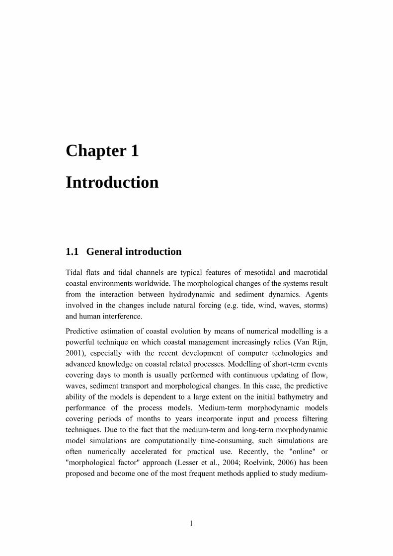
Tidal flats and tidal channels are typical features of mesotidal and macrotidal coastal environments worldwide. The morphological changes of the systems result from the interaction between hydrodynamic and sediment dynamics. Agents involved in the changes include natural forcing (e.g. tide, wind, waves, storms) and human interference.
Predictive estimation of coastal evolution by means of numerical modelling is a powerful technique on which coastal management increasingly relies (Van Rijn, 2001), especially with the recent development of computer technologies and advanced knowledge on coastal related processes. Modelling of short-term events covering days to month is usually performed with continuous updating of flow, waves, sediment transport and morphological changes. In this case, the predictive ability of the models is dependent to a large extent on the initial bathymetry and performance of the process models. Medium-term morphodynamic models covering periods of months to years incorporate input and process filtering techniques. Due to the fact that the medium-term and long-term morphodynamic model simulations are computationally time-consuming, such simulations are often numerically accelerated for practical use. Recently, the "online" or "morphological factor" approach (Lesser et al., 2004; Roelvink, 2006) has been proposed and become one of the most frequent methods applied to study medium-
1
Chapter 1. Introduction
and long-term morphological changes in nearshore environments (e.g. Dastgheib et al., 2008; Nguyen et al., 2010; Van der Wegen et al., 2010; Dissanayake et al., 2012; Tung et al., 2012). In this method, a ‘morphological factor’ (fMOR) is applied to increase the depth change rates by a constant factor at each computational time step. The predictive ability of the accelerated models, thus, depends to a large extent on the proper selection of the representative conditions and periods for the site under investigation.
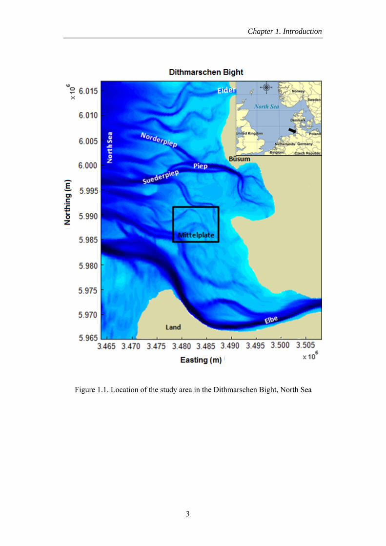
In this study, the medium-term morphodynamics of the tidal channel-flat system in the area of Mittelplate located in the Dithmarschen Bight, the German North Sea coast (Figure 1.1) is studied on the basis of field measurements and numerical modelling. The influence of an input reduction technique on simulated morphological evolution in the area on the medium-term time scale is also investigated.
1.2 Aim and objectives
The central aim of this thesis is to study the medium-term morphological evolution of the study area, which is characterized by a complex system of channels, flats and shoals. To achieve this aim, main research objectives are formulated as follows:
• Understanding the hydrodynamics and sediment dynamics of the investigated system;
• Improved understanding of the morphological evolution in medium-term in the study area;
• Identification of the roles of physical processes on the morphological development and
• Analysis of the influences of an input reduction technique and its applicability on simulating medium-term morphological evolution.
2
Chapter 1. Introduction
Figure 1.1. Location of the study area in the Dithmarschen Bight, North Sea
3
Chapter 1. Introduction
1.3 Outline of the thesis
The thesis consists of seven chapters; the descriptions of each chapter are briefly presented as follows:
Chapter 1 introduces the general topic and the objectives of this study.
Chapter 2 presents a literature review on morphodynamic processes and the main methods to study the morphological evolution of the coastal and estuary systems with emphasis to process-based morphodynamic modelling. In addition, an introduction to existing morphodynamic models and tools for assessing the model performance are also included.
In Chapter 3 the study area is described. The main characteristics of the hydrodynamics, sediment dynamics, sedimentology, and morphology are discussed. Data employed in the investigation are presented.
Chapter 4 focuses on investigating medium-term morphological evolution of the area based on field observations.
Chapter 5 presents the set-up, calibration, and validation of individual process models for simulation of flow, waves, and sediment transport of the Mittelplate area using Delft3D package. The Mittelplate morphodynamic model is then constructed on the basis of these process models.
Chapter 6 is devoted to study the medium-term morphodynamic evolution of the Mittelplate area based on the developed morphodynamic model. The effects of different forcing on the development of the area are illustrated.
Finally, main conclusions of the thesis and recommendations for further research are presented in Chapter 7.
4
Chapter 2
Literature review
2.1 Introduction
Wright and Thom (1977) defined coastal morphodynamics as mutual interactions and changes between morphology and hydrodynamic processes involving sediment transport. These hydrodynamic processes (tide- and wind-induced waves and tide-, wind- and wave-induced currents) cause sedimentation in some places and erosion in other elsewhere. The altered morphology, in turn, has effect on the driving forces themselves.
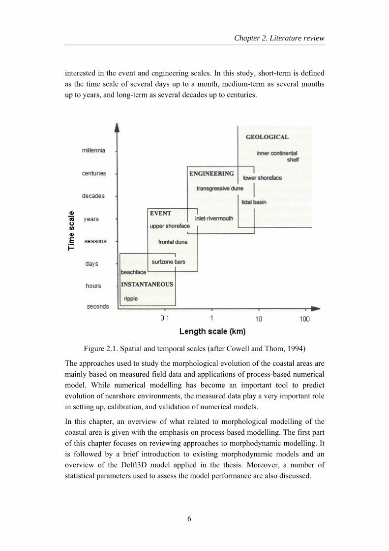
Morphodynamic processes are characterized by different spatial and temporal scales as shown in Figure 2.1. They are instantaneous, event, engineering, and geological scales with the time scales ranging from seconds to millennia. The different scales are not completely distinct, but overlap with each other. The smallest scale is instantaneous scale involving the time scale within which individual waves occur. This is the time frame for those processes like ripples formation. In the event scale, perturbations occur because of change in the parameters of the system and the system responds to those perturbations. For example, when a storm event having impact on morphological changes, the system can be recovered during the next storm event. The next level is the engineering scale, which is of interest in engineering projects. It concerns the coastal evolution in time frame of designed lifetime for coastal structures constructed in the area. The geological scale is the largest one, which concerns the coastal evolution spanning millennia. Coastal engineers and planners are usually
5
Chapter 2. Literature review
interested in the event and engineering scales. In this study, short-term is defined as the time scale of several days up to a month, medium-term as several months up to years, and long-term as several decades up to centuries.
Figure 2.1. Spatial and temporal scales (after Cowell and Thom, 1994)
The approaches used to study the morphological evolution of the coastal areas are mainly based on measured field data and applications of process-based numerical model. While numerical modelling has become an important tool to predict evolution of nearshore environments, the measured data play a very important role in setting up, calibration, and validation of numerical models.
In this chapter, an overview of what related to morphological modelling of the coastal area is given with the emphasis on process-based modelling. The first part of this chapter focuses on reviewing approaches to morphodynamic modelling. It is followed by a brief introduction to existing morphodynamic models and an overview of the Delft3D model applied in the thesis. Moreover, a number of statistical parameters used to assess the model performance are also discussed.
6
Chapter 2. Literature review
2.2 Approaches to morphodynamic modelling
De Vriend et al. (1993) categorized two approaches to morphological modelling of the coastal zone: ‘behaviour-oriented modelling’ and ‘process-based modelling’:
- Behavior oriented modelling: the idea is to map the behaviour of a coastal system on to a simple mathematical model which exhibits the same behaviour without describing the underlying physical processes.
- Process-based modelling: tides, waves, currents, sediment transport, and bed level changes are described through a set of mathematical equations. Since this study deals with the process-based modelling, emphasis will be on this approach.
Process-based model is the most widely used tool to simulate the coastal morphodynamics. Hydrodynamic models have reached a high degree of predictability due to the processes being fairly well understood. However, the sediment transport and morphodynamic models are considered to be in the process of development. The sand transport module generally is a critical key element and still requires a substantial input of information from empirical data sets; these data sets usually do not cover the total range of conditions and processes (Van Rijn et al., 2003).
When dealing with morphological issues of the coastal zone by application of process-based model, a fundamental problem is that the time scale of morphological evolution is much larger than that of the hydrodynamic processes. Reduction of information is therefore essential in medium-term and long-term modelling to make the computation within a feasible simulation time. A number of techniques with regards to this issue have been found in the literature. These include model reduction and input reduction which are described hereafter.
2.2.1 Model reduction
Model reduction, as introduced by De Vriend et al. (1993), is based on the idea that the model can be reformulated at the scale of interest without describing the details of the smaller-scale effects. Roelvink (2006) discussed several approaches of this type including tide-averaging approach in combination with the continuity correction, the Rapid Assessment of Morphology (RAM), and the online or morphological factor approach.
The tide-averaging approach considers the bottom fixed during the computation of hydrodynamics and sediment transport over a tidal cycle. The rate of change in
7
Chapter 2. Literature review
the bed level is computed from the gradients in the tidally averaged transport. The updated bathymetry is looped back to the transport model through the continuity correction or to the full hydrodynamics module. Within the continuity correction, the sediment transport field is adapted by adjusting the velocity and orbital velocity and recomputing the sediment transport which is a function of the velocity and the orbital velocity.
The RAM approach is an extension of the continuity correction method. The simplification is made by assuming that the transport field is dependent of only water depth.
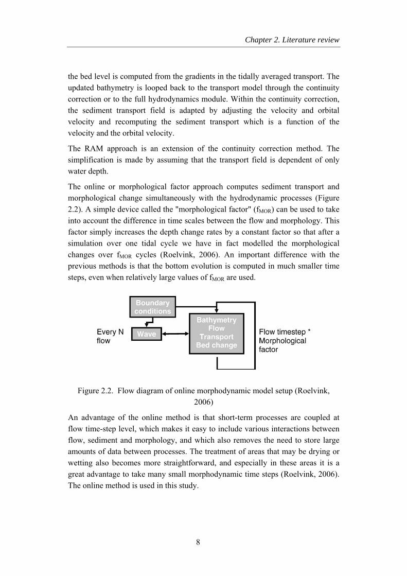
The online or morphological factor approach computes sediment transport and morphological change simultaneously with the hydrodynamic processes (Figure 2.2). A simple device called the "morphological factor" (fMOR) can be used to take into account the difference in time scales between the flow and morphology. This factor simply increases the depth change rates by a constant factor so that after a simulation over one tidal cycle we have in fact modelled the morphological changes over fMOR cycles (Roelvink, 2006). An important difference with the previous methods is that the bottom evolution is computed in much smaller time steps, even when relatively large values of fMOR are used.
Figure 2.2. Flow diagram of online morphodynamic model setup (Roelvink, 2006)
An advantage of the online method is that short-term processes are coupled at flow time-step level, which makes it easy to include various interactions between flow, sediment and morphology, and which also removes the need to store large amounts of data between processes. The treatment of areas that may be drying or wetting also becomes more straightforward, and especially in these areas it is a great advantage to take many small morphodynamic time steps (Roelvink, 2006). The online method is used in this study.
8
Chapter 2. Literature review
2.2.2 Input reduction
When applying any model reduction, input reduction is also needed in which the long-term residual sediment transport (or morphological change) patterns are obtained by applying models of smaller-scale processes driven by representative inputs. Input reduction is applied to tides, wind, and waves which is presented hereafter.
Latteux (1995) performed an investigation on the so-called "representative tide" using a 2D process-based model. One tide is selected to be representative for the bed evolution of a neap-spring tidal cycle or even a longer (19 years) cycle. He found that the best single tide was between mean and spring tide, leading to peak velocities about 12% larger than currents induced by mean tide. This tide raises an error on the bed evolution of about 6%. Within his study, he also investigated another way of simulating the yearly tidal cycle with a single tide. The result of this tide is multiplied by a factor chosen in such a way that the yearly evolution, averaged over the domain, is reproduced properly.
Bernades et al. (2006) proposed the so-called "ensemble technique" in which all tides in full tidal record are classified into classes according to their tidal range. Tides within each class are averaged. Different average tides are then linked in an ascending order as a continuous record. This record is then used as a boundary condition of the model in which sediment transport and bed level change are updated during the simulation. A scaling factor to the sediment transport is applied to each average tide depending on the frequency of occurrence of each average tide. The method was applied to simulate six-month morphological changes of Teign estuary, the United Kingdom and good results were reported.
The objective of wave input filtering is to represent the wave climate by a small number of representative conditions with which we can derive the wave model in our deterministic model system in order to estimate medium-term mean transports and bed evolutions (De Vriend et al., 1993). The authors reported two approaches, namely multiple and single representative wave approaches (MRW and SRW).
The multiple representative wave approach (MRW) was described by Steijn (1989, 1992). The wave (or wind field) data are reduced to a limited number of combinations of wave heights and directions. Those inputs are prescribed at the model boundary and the weight factor applied to the results of each of them in the calculation of medium-term mean transports and bed evolution. The criteria applied to determine these representative conditions and the corresponding weight factors refer to the two most prominent effects of waves on the transport: the bulk
9
Chapter 2. Literature review
longshore drift and the stirring of sediment. This approach works reasonable well in rather simple situations with not too wide a variety of transport mechanisms (De Vriend et al., 1993).
In the single representative wave approach (SRW), the results of wave computations for a number of sectors to yield a single set of representative wave parameters which is put into the flow and sediment transport models (Chesher and Miles, 1992). This would lead to a considerable saving in time and computational expense, since the flow and sand transport models would need to be run once only (De Vriend et al., 1993).
Comparing the two methods De Vriend et al. (1993) stated that they have their own limitation. The SRW approach rests exclusively upon the stirring effects of the waves so its applicability to situations with strong wave driven currents is not obvious. The MRW approach involves the risk of overlooking transports which occur under extreme condition as shown in Steijn (1992). The authors then recommended to use more wave height classes or separate schematizations for mean conditions and extreme events.
In addition, another method of input reduction based on the wind data was proposed by Boon et al. (2002). This is an approach of the current study and is presented separately in the following section.
2.3 Representative period method
The method "Representative Period” was proposed by Boon et al. (2002). The algorithm involved is used to select the time period (representative period) which the boundary conditions of the model are prescribed. The representative period (RP) is established on the basis of long-term records of wind data related to the area of concern. Three “Cost Functions” are constructed:
C1 = (Wn - Wn_lt)2 + (We - We_lt)2 (2.1)
C2 = (σWn - σWn_lt)2 + (σWe - σWe_lt)2 (2.2)
C3 = C1/σC1 + C2/σC2 (2.3)
where: Wn, We RP averaged north and east wind components Wn_lt , We_lt long-term averaged north and east wind components σ standard deviation
10
Chapter 2. Literature review
According to Boon et al. (2002) the representative period of the investigated time series is the period pertaining to the lowest value of the cost function C3.
Applying the method, Boon et al. (2002) performed six dumping scenario simulations using Delft3D model for the Ems-Dollard estuary, southern North Sea coast over a period of two months. They concluded that the model is capable to simulate the sediment dynamic behaviour and the impact of the alternative dumping locations adequately.
Nguyen et al. (2010) applied the method to reduce the input data to study migration of a channel on the German North Sea coast with the help of Delft3D model. Morphodynamic simulations were carried out for the periods of two and four years, and good results were reported.
Jimenez (2011) carried out a method to investigate morphological changes in the Luebeck Bay, German Baltic Sea over a period of one year, separating the storm and calm periods. With the application of MIKE 21 modelling system, the storm period is initially simulated assuming the conditions of one storm as representative. Subsequently, the morphological simulations for a period of calm conditions were carried applying the morphological factor technique and representative period method. Although the morphological model has not been calibrated and validated, the author concluded that the results are consistent with the expected changes during the transformation of the coastal zones.
2.4 Process-based morphodynamic models
The continuous interaction between a number of constituent processes waves, currents, and sediment transport results in coastal morphology and multidimensional coastal evolution models usually start from a number of more or less standard models of those processes. The "state of art” on the present knowledge of morphodynamic processes is reflected by the current generation of mathematical, process-based models (Van Rijn et al., 2003). Over the last decades, efforts have been made in developing morphodynamic models to predict the sediment transport rates and resulting bed evolution of complex coastal and estuarine environments. The process-based morphodynamic models usually consist of modules: hydrodynamic, sediment transport and bottom updating modules. They are implemented in a loop so that feedbacks are made among the elements of the morphodynamic system.
11
Chapter 2. Literature review
Most existing morphodynamic models are based on finite difference methods (e.g. Delft3D, XBeach, ROMS), finite element methods (e.g TELEMAC, TIMOR), or finite volume methods (e.g. MIKE21). In finite difference methods, the structured grids (rectangular or curvilinear) are used, while unstructured grids (triangles or a combination of triangles and quadrilaterals) are used in finite element methods and finite volume methods. The followings will present brief review of several well-known morphodynamic process-based models which are applied to the coastal environment.
• Delft3D (Lesser et al., 2004) is a 2D/3D integrated modelling system developed by Deltares (formerly known as WL|Delft Hydraulics). It consists of several modules for the physical processes: waves, currents, sediment transport, bottom changes, and water quality. The Delft3D model will be used in this study. More detailed description will be given in next section.
• MIKE 21 (Warren and Bach, 1992), which has been developed by DHI (Danish Hydraulic Institute) Denmark, is a 2D comprehensive modelling system for the simulation of flows, waves, sediment transport in estuaries, coastal areas, and seas.
• ROMS (Warner et al., 2008) is a three-dimensional numerical model, which implements algorithms for sediment transport and evolution of bottom morphology in the coastal-circulation model Regional Ocean Modeling System. The coupled model between ROMS and wave model Simulating Waves in the Nearshore (SWAN) is applicable for fluvial, estuarine, shelf, and nearshore environments.
• TELEMAC (Villaret et al., 2011), which was developed by the National Hydraulics and Environment Laboratory of the Research and Development Directorate of the French Electricity Board, is a 2D/3D modelling system for free surface waters. The sediment transport module of the modelling system SISYPHE can be tightly coupled with hydrodynamic model TELEMAC-2D and TELEMAC-3D while including inputs from the wave model TOMAWAC to enable morphodynamic modelling.
• TIMOR package (Zanke and Mewis, 2002) has been developed at the Institute of Hydraulics and Water Resources at the Technical University of Darmstadt. It is a 3D dynamic modelling system that simulates the flow and sediment transport in lakes, estuaries, harbours, and coastal waters under the forcing of wind, tides, freshwater inflows, and density gradients with the influence of the Coriolis acceleration, complex bathymetry and shoreline geometry.
12
Chapter 2. Literature review
• XBeach (Roelvink et al., 2009) is a 2D morphological model, which has been developed by a consortium of UNESCO-IHE, Deltares, Delft University of Technology, and the University of Miami with funding and support by the US Army Corps of Engineers. It is used to assess the natural coastal response to time varying storm and hurricane conditions, including dune erosion, overwash, and breaching.
2.5 Delft3D model
The study applies Delft3D modelling system, which has been developed by Deltares. It consists of several modules for the physical processes: waves, currents, sediment transport, bottom changes, and water quality. Since the current research focuses on a depth-averaged case, the following sections will present the main model characteristics applied in 2D depth-averaged mode. More information can be found in Lesser et al. (2004) and Deltares (2008a, b).
2.5.1 Hydrodynamic model
Hydrodynamic equations
The hydrodynamic model solves the Navier-Stokes equations for an incompressible fluid under the shallow water and the Boussinesq assumption.
The depth-averaged continuity equation is given by:
( ) ( ) 0d u d vt x yη η η∂ ∂ + ∂ +
+ +∂ ∂ ∂
= (2.4)
Conservation of momentum in x and y directions (depth and density averaged):
2 2
2 2
U0
C ( ) ( )x
w
gu Fu u u uu g fv vt x x d d x
vy
uy
ηη ρ η
∂ ⎛ ⎞∂ ∂ ∂ ∂ ∂+ + − + − − + =⎜∂ ∂ ∂ + + ∂ ∂⎝ ⎠
+∂ 2 ⎟ (2.5)
2 2
2 2
U0
C ( ) ( )y
w
Fgvv v v vu g fu vt x y d d
vy yv
xη
η ρ η∂ ⎛ ⎞∂ ∂ ∂ ∂ ∂
+ + − + − − + =⎜∂ ∂ ∂ + + ∂ ∂⎝ ⎠+
∂ 2 ⎟ (2.6)
where:
C Chézy coefficient
d bottom depth
13
Chapter 2. Literature review
f Coriolis parameter
Fx, Fy x- and y-component of external forces
u, v depth averaged velocity in x- and y-direction
U = 2 2u v+
ρw mass density of water
ν horizontal viscosity
η water level above reference level
g gravity of acceleration
Grid structure
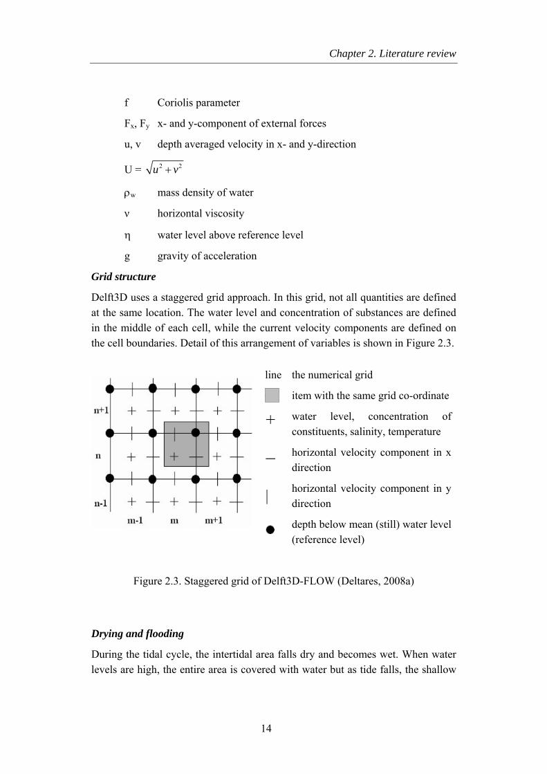
Delft3D uses a staggered grid approach. In this grid, not all quantities are defined at the same location. The water level and concentration of substances are defined in the middle of each cell, while the current velocity components are defined on the cell boundaries. Detail of this arrangement of variables is shown in Figure 2.3.
line
+
_
⏐
the numerical grid
item with the same grid co-ordinate
water level, concentration of constituents, salinity, temperature
horizontal velocity component in x direction
horizontal velocity component in y direction
depth below mean (still) water level (reference level)
Figure 2.3. Staggered grid of Delft3D-FLOW (Deltares, 2008a)
Drying and flooding
During the tidal cycle, the intertidal area falls dry and becomes wet. When water levels are high, the entire area is covered with water but as tide falls, the shallow
14
Chapter 2. Literature review
areas are exposed, and ultimately the flow is confined only to the deeper channels. The dry tidal flats may occupy a substantial fraction of the total surface area. The accurate reproduction of covering or uncovering of the tidal flats is an important feature of numerical flow models based on the shallow water equations.
In a numerical model, the process of drying and flooding is represented by removing grid points from the flow domain that become "dry" when the tide falls and by adding grid points that become "wet" when the tide rises. Drying and flooding is constrained to follow the sides of grid cells.
2.5.2 Wave model
Two wave models are available in Delft3D: HISWA (HIndcast of Shallow-water Waves) wave model (Holthuijsen et al., 1989) and SWAN (Simulating WAves Nearshore) wave model (Booij et al., 1999; Ris et al., 1999). The third-generation SWAN model is the successor of the stationary second-generation HISWA model.
This study makes use of the SWAN wave model because SWAN model has some more advantages compared to HISWA as follows:
• SWAN can perform computations on a curvilinear grid, which results in better coupling with the FLOW module of Delft3D, whereas HISWA is limited to rectilinear grids.
• The computational grid in SWAN has not to be oriented in the mean wave direction as in the HISWA model.
• The wave forces can be computed on the gradient of the radiation stress tensor rather than on the dissipation rate as in the HISWA model.
• The physics in SWAN are explicitly represented with state-of-art formulations, while HISWA uses highly parameterised formulations.
• The SWAN model is fully spectral in frequencies and directions, whereas the HISWA model is parameterised in frequency, which does not allow for the simulation of multi-modal wave fields.
In SWAN the waves are described with the two-dimensional wave action density spectrum. Since in the presence of currents, action density conserved, whereas energy density is not, the spectrum considered in SWAN is the action density spectrum N (σ,θ) rather than the energy density spectrum E (σ,θ), which:
σθσ
θσ),(),( EN =
(2.7)
15
Chapter 2. Literature review
The evolution of wave spectrum for Cartesian coordinate is:
σθσθσ
θθσ
σθσθσθσ θσ
),(),(),(),(),(),( SNcNcNcy
Ncx
Nt yx =
∂∂
+∂∂
+∂∂
+∂∂
+∂∂
(2.8)
in which:
σ, θ the relative frequency and direction
cx, cy the energy transport velocity in the geographical space (x,y)
cσ, cθ the energy transport velocity in the spectral space (σ,θ)
S (σ,θ) the source term in terms of energy density representing the effects of generation, dissipation, and non-linear wave-wave interactions
2.5.3 Sediment transport model
The sediment transport and morphology module supports both bed-load and suspended load transport of non-cohesive sediments and suspended load of cohesive sediments.
Suspended sediment
Suspended sediment is calculated by solving the advection-diffusion (mass-balance) equation for the suspended sediment:
hSycD
yxcD
xhhvc
yhuc
xhc
t+⎥
⎦
⎤⎢⎣
⎡⎟⎟⎠
⎞⎜⎜⎝
⎛∂∂
∂∂
+⎟⎠⎞
⎜⎝⎛
∂∂
∂∂
=∂∂
+∂∂
+∂∂
(2.9)
where:
c depth-averaged sediment concentration
S sediment source term
D horizontal diffusion coefficient
For cohesive sediment fractions, the fluxes between the water phase and the bed are calculated with the well-known Partheniades-Krone formulations (Partheniades, 1965):
( )ecrcweMSE ,,ττ= (2.10)
( )dcrcwdbs ScwD ,,ττ= (2.11)
where:
16
Chapter 2. Literature review
E erosion flux [kg m-2s-1]
M erosion parameter [kg m-2s-1]
( )ecrcweS ,,ττ erosion step function:
( )⎪⎪⎩
⎪⎪⎨
⎧
≤
>⎟⎟⎠
⎞⎜⎜⎝
⎛−
=
ecrcw
ecrcwecr
cw
ecrcwe
when
whenS
,
,,
,
0
1,
ττ
ττττ
ττ (2.12)
D deposition flux [kg m-2s-1]
ws sediment fall velocity [m/s]
cb average sediment concentration in the near bottom computational layer [kg/m3]
( )dcrcwdS ,,ττ deposition step function:
( )⎪⎪⎩
⎪⎪⎨
⎧
≥
<⎟⎟⎠
⎞⎜⎜⎝
⎛−
=
dcrcw
dcrcwdcr
cw
dcrcwd
when
whenS
,
,,
,
0
1,
ττ
ττττ
ττ (2.13)
τcw maximum shear stress due to waves and current [N/m2]
τcr,e critical shear stress for erosion [N/m2]
τcr,d critical shear stress for deposition [N/m2]
Bed load transport
Within this study, bed load transport is computed for sand sediment fraction following the method of Van Rijn (1993), which includes the effect of waves. This accounts for the near-bed sediment transport occurring below the reference height.
The magnitude of bed-load transport is computed as:
(2.14) 7.05.050006.0 essb MMdwS ρ=
where:
Sb bed load transport [kg/m/s]
M sediment mobility number due to waves and currents [-]
17

Chapter 2. Literature review
Me excess sediment mobility number [-]
50
2
)1( gdsv
M eff
−= (2.15)
( )
50
2
)1( gdsvv
M creffe −
−= (2.16)
22onReff Uvv += (2.17)
in which:
vcr critical depth averaged velocity for initiation of motion (based on a parameterisation of the Shields curve) [m/s]
vR magnitude of an equivalent depth-averaged velocity computed from the velocity in the bottom computational layer, assuming a logarithmic velocity profile [m/s]
Uon near-bed peak orbital velocity [m/s] in onshore direction (in the direction on wave propagation) based on the significant wave height
Suspended sediment correction vector
The transport of suspended sediment is computed over the entire water column. However, for "sand" sediment fractions, Van Rijn (1993) regards sediment transported below the reference height ‘a’ as belonging to "bed-load sediment transport" which is computed separately as it responds almost instantaneously to changing flow conditions and feels the effects of bed slopes. In order to prevent double counting, the suspended sediment fluxes below the reference height a are derived by means of numerical integration from the suspended transport rates. The opposite of these fluxes are scaled with the upwind sediment availability and subsequently imposed as corrective transport.
2.5.4 Morphodynamic model
The elevation of the bed is dynamically updated at each computational time-step. It means that the hydrodynamic flow calculations are always carried out using the correct bathymetry. At each time-step, the change in the mass of bed material that has occurred as a result of the sediment sink and source terms and transport gradients is calculated. This change in mass is then translated into a bed level change based on the dry bed densities of the various sediment fractions. Both the bed levels at the cell centres and cell interfaces are updated.
18
Chapter 2. Literature review
Total change in bed
The total change in sediment is the sum of change due to suspended load, suspended load correction vector and bed load.
Suspended sediment transport
The net sediment change due to suspended sediment transport is determined as:
(2.18) tSourceSinkfs MORnm
sus ∆−=∆ )(,
where:
fMOR morphological acceleration factor
∆t computational time step [s]
The correction of suspended sediment transport below the reference height is calculated as:
),(),(,
,)1,(1,
,
),(,,
),1(,1,),(
nmnmnmvvcor
nmnmvvcor
nmnmuucor
nmnmuucor
MORnm
cor At
xSxSySyS
fs ∆⎟⎟⎠
⎞⎜⎜⎝
⎛
∆−∆+∆−∆
=∆ −−
−−
(2.19)
A(m,n) area of computational cell at location (m, n) [m2].
, suspended sediment correction vector components in u, v directions [kg/(m s)]
nmuucorS ,
,nmvvcorS ,
,
, cell width in the x and y directions [m] ),( nmx∆ ),( nmy∆
Bed-load sediment transport
The change in quantity of bottom sediments caused by bed-load transport is calculated as:
),(),(,
,)1,(1,
,
),(,,
),1(,1,),(
nmnmnmvvb
nmnmvvb
nmnmuub
nmnmuub
MORnm
bed At
xSxSySyS
fs ∆⎟⎟⎠
⎞⎜⎜⎝
⎛
∆−∆+∆−∆
=∆ −−
−−
(2.20)
where:
and bed load sediment transport vector components at the u and v velocity points [kg/(m s)]
19
Chapter 2. Literature review
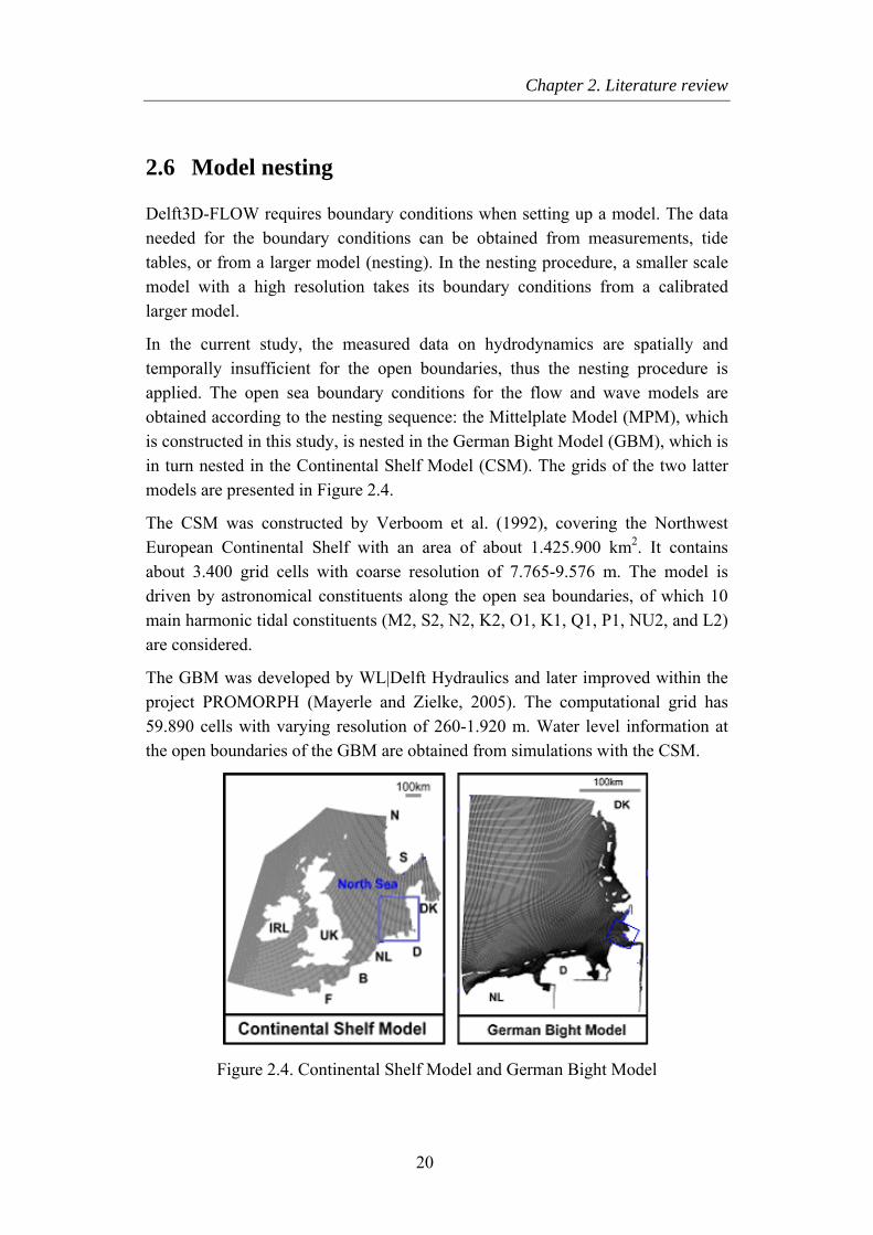
2.6 Model nesting
Delft3D-FLOW requires boundary conditions when setting up a model. The data needed for the boundary conditions can be obtained from measurements, tide tables, or from a larger model (nesting). In the nesting procedure, a smaller scale model with a high resolution takes its boundary conditions from a calibrated larger model.
In the current study, the measured data on hydrodynamics are spatially and temporally insufficient for the open boundaries, thus the nesting procedure is applied. The open sea boundary conditions for the flow and wave models are obtained according to the nesting sequence: the Mittelplate Model (MPM), which is constructed in this study, is nested in the German Bight Model (GBM), which is in turn nested in the Continental Shelf Model (CSM). The grids of the two latter models are presented in Figure 2.4.
The CSM was constructed by Verboom et al. (1992), covering the Northwest European Continental Shelf with an area of about 1.425.900 km2. It contains about 3.400 grid cells with coarse resolution of 7.765-9.576 m. The model is driven by astronomical constituents along the open sea boundaries, of which 10 main harmonic tidal constituents (M2, S2, N2, K2, O1, K1, Q1, P1, NU2, and L2) are considered.
The GBM was developed by WL|Delft Hydraulics and later improved within the project PROMORPH (Mayerle and Zielke, 2005). The computational grid has 59.890 cells with varying resolution of 260-1.920 m. Water level information at the open boundaries of the GBM are obtained from simulations with the CSM.
Figure 2.4. Continental Shelf Model and German Bight Model
20
Chapter 2. Literature review
2.7 Meteorological models
In this study, the metrological data including wind and atmospheric pressure are obtained from the synoptic PRISMA model (Luthardt, 1987) for the period of 1996-2000 and from COSMO-Model (Schättler et al., 2009) for the period 2000-2009.
PRISMA has been developed at the Max Planck Institute of Meteorology of the University of Hamburg to generate wind and pressure fields covering the entire North Sea. The PRISMA data consist of wind speeds and pressures at three-hour intervals on a regular mesh spacing of 42 km.
COSMO-Model (formerly known as Lokal Modell - LM) has been developed at the German Weather Service (DWD). It is a nonhydrostatic limited-area atmospheric prediction model with different grid resolutions. In this study, output data of wind forcing and atmospheric pressure from the COSMO model with the temporal resolution of one hour and spatial resolution of 7 km have been used.
2.8 Statistical parameters for evaluation of model performance
Evaluating the performance of numerical models of coastal morphology against observations is an essential part of establishing their credibility (Sutherland et al., 2004). In this study, the performance of the models is evaluated through qualitative and quantitative manners, involving both graphical comparisons and statistical tests. This section presents a number of statistical parameters used to assess the model performance.
2.8.1 Statistical parameters in hydrodynamic modelling
Let xm be a set of n measured values and xc be a set of n calculated values, <> indicates the time average procedure. The mean Absolute Error (MAE), the Mean Square Error (MSE), and Relative Mean Absolute Error (RMAE) are defined as:
mc xxMAE −= (2.21)
( )2mc xxMSE −= (2.22)
21
Chapter 2. Literature review
( )2mc xxRMSE −= (2.23)
mmc xxxRMAE /−= (2.24)
RMSE is often preferred to MSE as it has the same units as the measured variable. The use of the modulus makes MAE nonanalytic and thus more difficult to manipulate mathematically than MSE or RMSE (Sutherland et al., 2004). However, the MAE is equally applicable to vectors and scalars, and so is particularly useful for validating and evaluating hydrodynamic modeling (Sutherland et al., 2004). The authors also pointed out that RMSE is greater than or equal to the MAE so RMSE is a more conservative error predictor. The Relative Mean Absolute Error is preferred above the Relative Mean Square Error, because the presence of a few outliers will have a greater influence on RMSE than on RMAE as RMSE squares the differences. The RMAE is therefore less susceptible to the presence of outliers (Van Rijn et al., 2003).
Van Rijn et al. (2003) proposed to evaluate the performance of the hydrodynamic models on the basis of the RMAE that considers the error of measured parameter. The author also proposed the qualitative ranking based on the value ranges of RMAE as shown in the Table 2.1.
mmmc xxxxRMAE /∆−−= (2.25)
where:
∆xm error of measured parameter
RMAE of wave height, current velocity are corrected for the measurement errors, being ∆xm = 0.1 m for wave height, ∆xm = 0.05 m/s for current velocity.
Table 2.1. Qualification of RMAE (Van Rijn et al., 2003)
Qualification Wave height RMAE Velocity RMAE
Excellent < 0.05 < 0.1
Good 0.05 – 0.1 0.1 – 0.3
Reasonable/fair 0.1 – 0.2 0.3 – 0.5
Poor 0.2 – 0.3 0.5 – 0.7
Bad > 0.3 > 0.7
22
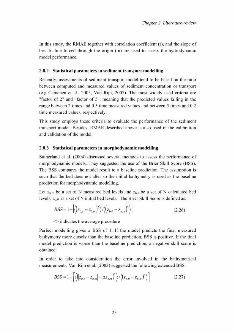
Chapter 2. Literature review
In this study, the RMAE together with correlation coefficient (r), and the slope of best-fit line forced through the origin (m) are used to assess the hydrodynamic model performance.
2.8.2 Statistical parameters in sediment transport modelling
Recently, assessments of sediment transport model tend to be based on the ratio between computed and measured values of sediment concentration or transport (e.g Camenen et al., 2005, Van Rijn, 2007). The most widely used criteria are "factor of 2" and "factor of 5", meaning that the predicted values falling in the range between 2 times and 0.5 time measured values and between 5 times and 0.2 time measured values, respectively.
This study employs those criteria to evaluate the performance of the sediment transport model. Besides, RMAE described above is also used in the calibration and validation of the model.
2.8.3 Statistical parameters in morphodynamic modelling
Sutherland et al. (2004) discussed several methods to assess the performance of morphodynamic models. They suggested the use of the Brier Skill Score (BSS). The BSS compares the model result to a baseline prediction. The assumption is such that the bed does not alter so the initial bathymetry is used as the baseline prediction for morphodynamic modelling.
Let zb,m be a set of N measured bed levels and zb,c be a set of N calculated bed levels, zb,0 is a set of N initial bed levels. The Brier Skill Score is defined as:
( ) ( )[ ]2,0,
2,, /1 mbbmbcb zzzzBSS −−−= (2.26)
<> indicates the average procedure
Perfect modelling gives a BSS of 1. If the model predicts the final measured bathymetry more closely than the baseline prediction, BSS is positive. If the final model prediction is worse than the baseline prediction, a negative skill score is obtained.
In order to take into consideration the error involved in the bathymetrical measurements, Van Rijn et al. (2003) suggested the following extended BSS:
( ) ( ) ⎥⎦⎤
⎢⎣⎡ −∆−−−= 2
,0,2
,,, /1 mbbmbmbcb zzzzzBSS (2.27)
23
Chapter 2. Literature review
where:
∆zb,m measurement error of bed level. ∆zb,m = 0.1 m for bed level in field conditions and 0.02 m for laboratory conditions.
In this study, for the purpose of quantifying the accelerated simulations using representative periods in comparison with the benchmark simulations (Chapter 6), the BSS is adjusted as follows:
( ) ( ) ⎥⎦⎤
⎢⎣⎡ −−−= 2
,0,2
,, /1 BSbbBSbASb zzzzBSS (2.28)
where:
zb,AS computed bed level from accelerated simulation
zb,BS computed bed level from benchmark simulation
zb,0 initial bed level
A BSS value of 1 indicates a perfect match between the predicted bed levels of benchmark run and accelerated run. BSS values lower than 1 implies a difference between bed levels predicted by the two runs. The BSS can be smaller than 0 when the model result is less accurate than the baseline run. The qualification of the model based on BSS is presented in Table 2.2.
Table 2.2. Qualification of BSS (Van Rijn et al., 2003)
Qualification BSS
Excellent 1.0 – 0.8
Good 0.8 – 0.6
Reasonable/fair 0.6 – 0.3
Poor 0.3 – 0
Bad < 0
24
Chapter 3
Study area and available data
3.1 Introduction
The study concerns the Mittelplate area on the Dithmarschen Bight, the German North Sea coast (Figure 1.1). The Dithmarschen Bight comprises the tidal flats, tidal channels, and sand banks between Eider and Elbe rivers. The tidal flats and sandbanks are exposed at low water which approximately 50% of the area falls dry at low tide (Mayerle and Zielke, 2005).
Focus of the thesis will be on the tidal flat-tidal channel system in the Mittelplate area, which is about 12 km south of Piep channel system (Figure 3.1). The Trischenflinge channel is about 7 km long, connecting the Neufahrwasser channel located to the north at its southeastern end. The tidal flat is located between the two channels where an oil platform is present. The width of the Trischenflinge channel varies spatially and temporally from about 100 m to 400 m related to the 4 m depth contour. The maximum depth of the channel was measured to about 12 m in the year 2008.
25
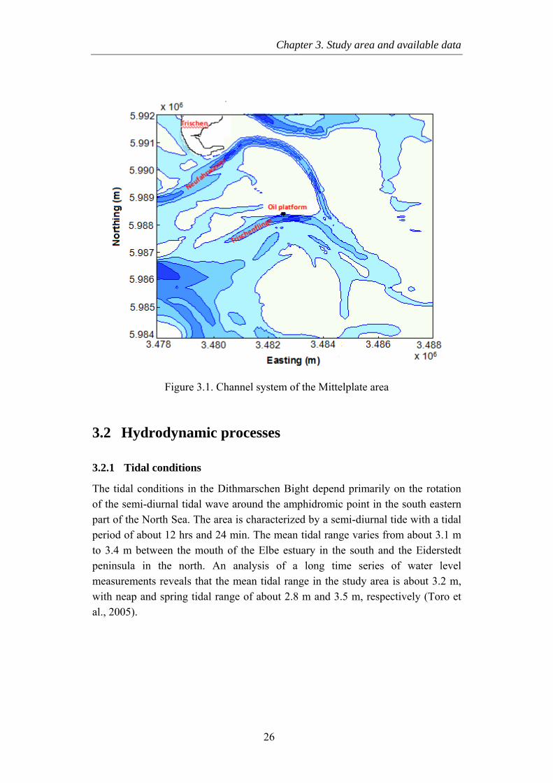
Chapter 3. Study area and available data
Figure 3.1. Channel system of the Mittelplate area
3.2 Hydrodynamic processes
3.2.1 Tidal conditions
The tidal conditions in the Dithmarschen Bight depend primarily on the rotation of the semi-diurnal tidal wave around the amphidromic point in the south eastern part of the North Sea. The area is characterized by a semi-diurnal tide with a tidal period of about 12 hrs and 24 min. The mean tidal range varies from about 3.1 m to 3.4 m between the mouth of the Elbe estuary in the south and the Eiderstedt peninsula in the north. An analysis of a long time series of water level measurements reveals that the mean tidal range in the study area is about 3.2 m, with neap and spring tidal range of about 2.8 m and 3.5 m, respectively (Toro et al., 2005).
26
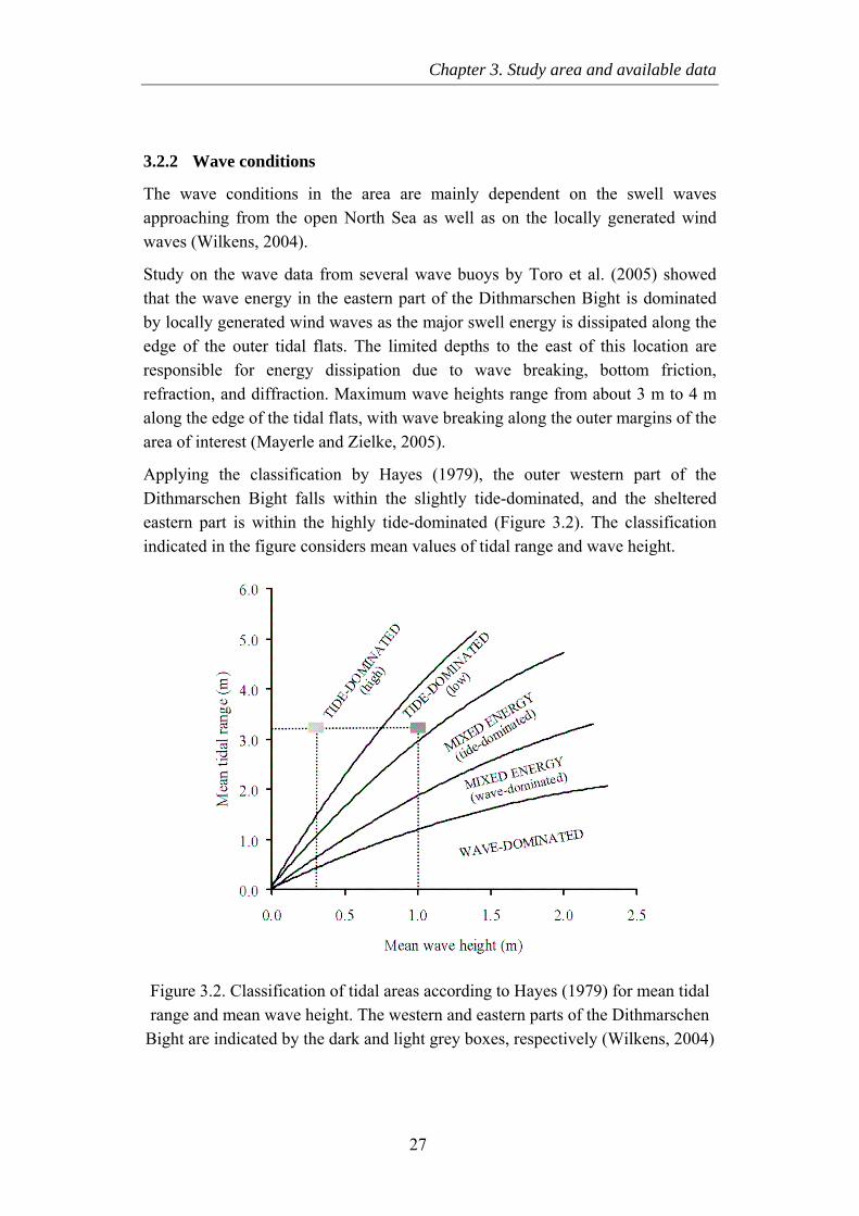
Chapter 3. Study area and available data
3.2.2 Wave conditions
The wave conditions in the area are mainly dependent on the swell waves approaching from the open North Sea as well as on the locally generated wind waves (Wilkens, 2004).
Study on the wave data from several wave buoys by Toro et al. (2005) showed that the wave energy in the eastern part of the Dithmarschen Bight is dominated by locally generated wind waves as the major swell energy is dissipated along the edge of the outer tidal flats. The limited depths to the east of this location are responsible for energy dissipation due to wave breaking, bottom friction, refraction, and diffraction. Maximum wave heights range from about 3 m to 4 m along the edge of the tidal flats, with wave breaking along the outer margins of the area of interest (Mayerle and Zielke, 2005).
Applying the classification by Hayes (1979), the outer western part of the Dithmarschen Bight falls within the slightly tide-dominated, and the sheltered eastern part is within the highly tide-dominated (Figure 3.2). The classification indicated in the figure considers mean values of tidal range and wave height.
Figure 3.2. Classification of tidal areas according to Hayes (1979) for mean tidal range and mean wave height. The western and eastern parts of the Dithmarschen
Bight are indicated by the dark and light grey boxes, respectively (Wilkens, 2004)
27
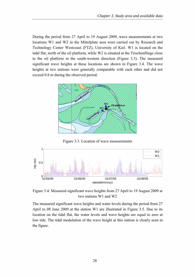
Chapter 3. Study area and available data
During the period from 27 April to 19 August 2009, wave measurements at two locations W1 and W2 in the Mittelplate area were carried out by Research and Technology Center Westcoast (FTZ), University of Kiel. W1 is located on the tidal flat, north of the oil platform, while W2 is situated at the Trischenflinge close to the oil platform in the south-western direction (Figure 3.3). The measured significant wave heights at these locations are shown in Figure 3.4. The wave heights at two stations were generally comparable with each other and did not exceed 0.8 m during the observed period.
Figure 3.3. Location of wave measurements
01/05/09 01/06/09 01/07/09 01/08/090
0.5
1
date(dd/mm/yy)
H
W2W1
s(m)
Hs
(m)
Figure 3.4. Measured significant wave heights from 27 April to 19 August 2009 at two stations W1 and W2
The measured significant wave heights and water levels during the period from 27 April to 08 June 2009 at the station W1 are illustrated in Figure 3.5. Due to its location on the tidal flat, the water levels and wave heights are equal to zero at low tide. The tidal modulation of the wave height at this station is clearly seen in the figure.
28
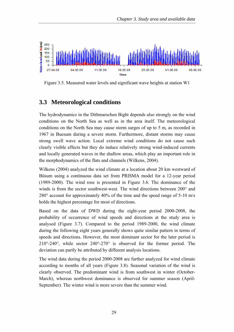
Chapter 3. Study area and available data
Figure 3.5. Measured water levels and significant wave heights at station W1
3.3 Meteorological conditions
The hydrodynamics in the Dithmarschen Bight depends also strongly on the wind conditions on the North Sea as well as in the area itself. The meteorological conditions on the North Sea may cause storm surges of up to 5 m, as recorded in 1967 in Buesum during a severe storm. Furthermore, distant storms may cause strong swell wave action. Local extreme wind conditions do not cause such clearly visible effects but they do induce relatively strong wind-induced currents and locally generated waves in the shallow areas, which play an important role in the morphodynamics of the flats and channels (Wilkens, 2004).
Wilkens (2004) analyzed the wind climate at a location about 20 km westward of Büsum using a continuous data set from PRISMA model for a 12-year period (1989-2000). The wind rose is presented in Figure 3.6. The dominance of the winds is from the sector southwest-west. The wind directions between 200° and 280° account for approximately 40% of the time and the speed range of 5-10 m/s holds the highest percentage for most of directions.
Based on the data of DWD during the eight-year period 2000-2008, the probability of occurrence of wind speeds and directions at the study area is analysed (Figure 3.7). Compared to the period 1989-2000, the wind climate during the following eight years generally shows quite similar pattern in terms of speeds and directions. However, the most dominant sector for the later period is 210°-240°, while sector 240°-270° is observed for the former period. The deviation can partly be attributed by different analysis locations.
The wind data during the period 2000-2008 are further analyzed for wind climate according to months of all years (Figure 3.8). Seasonal variation of the wind is clearly observed. The predominant wind is from southwest in winter (October-March), whereas northwest dominance is observed for summer season (April-September). The winter wind is more severe than the summer wind.
29
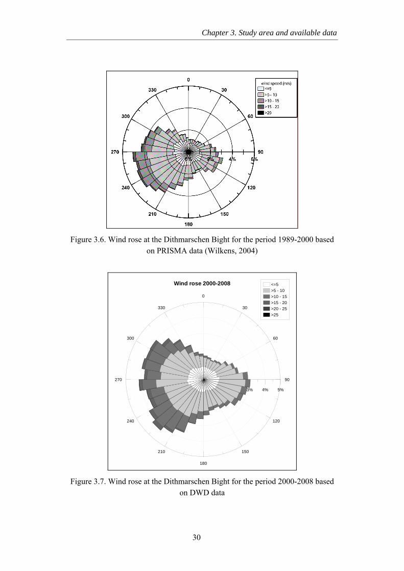
Chapter 3. Study area and available data
Figure 3.6. Wind rose at the Dithmarschen Bight for the period 1989-2000 based on PRISMA data (Wilkens, 2004)
0
30
60
90
120
150
180
210
240
270
300
330
0% 1% 2% 3% 4% 5%
<=5>5 - 10>10 - 15>15 - 20>20 - 25>25
Wind rose 2000-2008
Figure 3.7. Wind rose at the Dithmarschen Bight for the period 2000-2008 based on DWD data
30
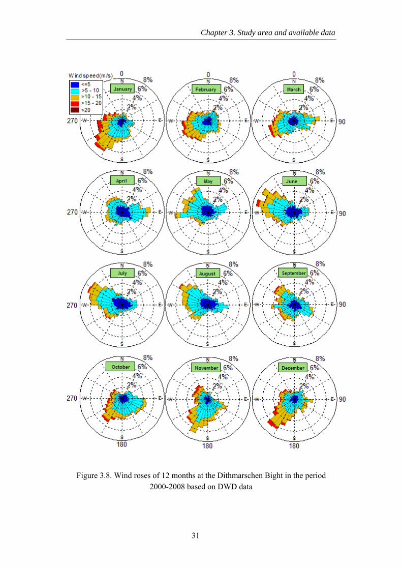
Chapter 3. Study area and available data
Figure 3.8. Wind roses of 12 months at the Dithmarschen Bight in the period 2000-2008 based on DWD data
31
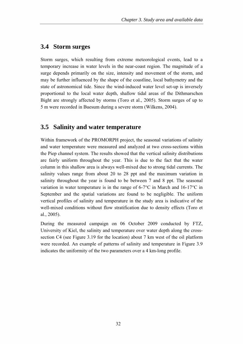
Chapter 3. Study area and available data
3.4 Storm surges
Storm surges, which resulting from extreme meteorological events, lead to a temporary increase in water levels in the near-coast region. The magnitude of a surge depends primarily on the size, intensity and movement of the storm, and may be further influenced by the shape of the coastline, local bathymetry and the state of astronomical tide. Since the wind-induced water level set-up is inversely proportional to the local water depth, shallow tidal areas of the Dithmarschen Bight are strongly affected by storms (Toro et al., 2005). Storm surges of up to 5 m were recorded in Buesum during a severe storm (Wilkens, 2004).
3.5 Salinity and water temperature
Within framework of the PROMORPH project, the seasonal variations of salinity and water temperature were measured and analyzed at two cross-sections within the Piep channel system. The results showed that the vertical salinity distributions are fairly uniform throughout the year. This is due to the fact that the water column in this shallow area is always well-mixed due to strong tidal currents. The salinity values range from about 20 to 28 ppt and the maximum variation in salinity throughout the year is found to be between 7 and 8 ppt. The seasonal variation in water temperature is in the range of 6-7°C in March and 16-17°C in September and the spatial variations are found to be negligible. The uniform vertical profiles of salinity and temperature in the study area is indicative of the well-mixed conditions without flow stratification due to density effects (Toro et al., 2005).
During the measured campaign on 06 October 2009 conducted by FTZ, University of Kiel, the salinity and temperature over water depth along the cross-section C4 (see Figure 3.19 for the location) about 7 km west of the oil platform were recorded. An example of patterns of salinity and temperature in Figure 3.9 indicates the uniformity of the two parameters over a 4 km-long profile.
32
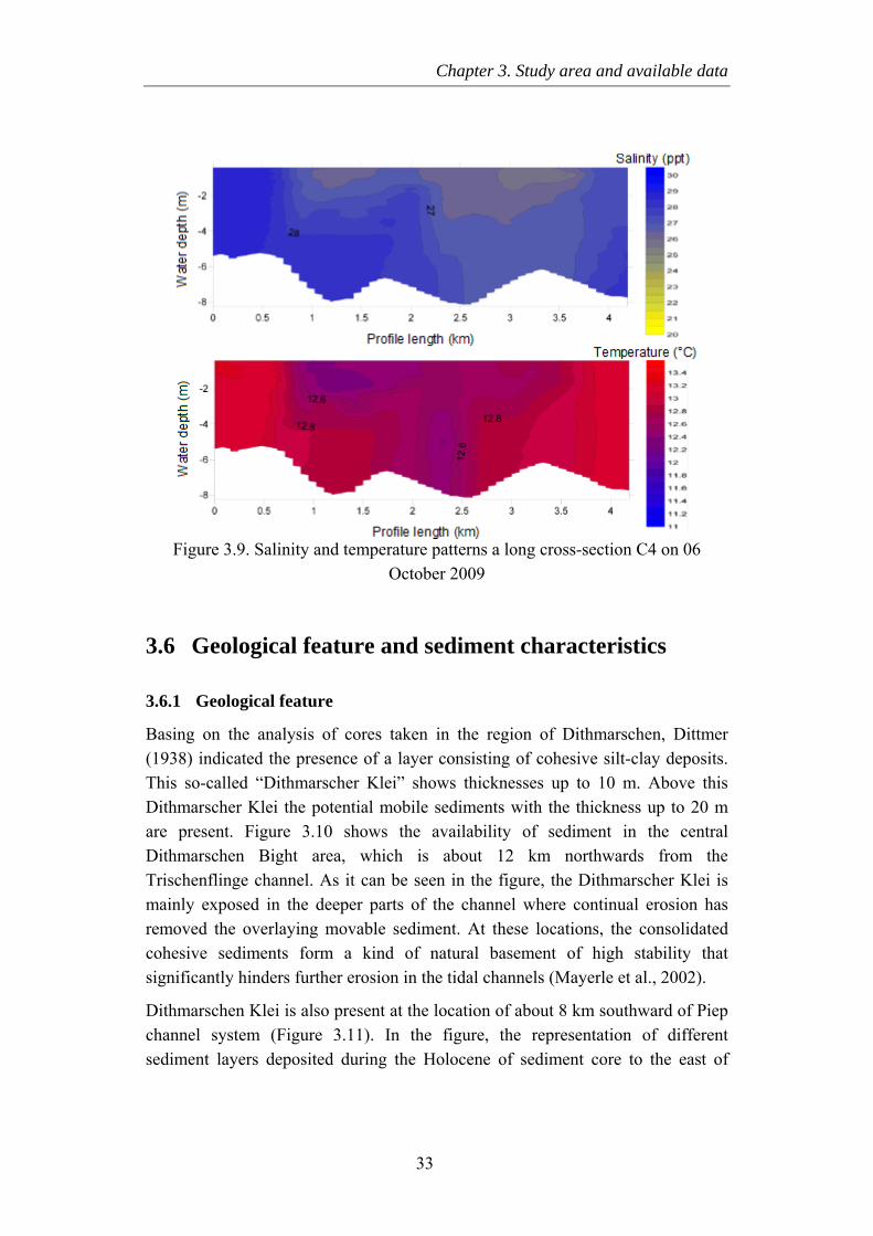
Chapter 3. Study area and available data
Figure 3.9. Salinity and temperature patterns a long cross-section C4 on 06
October 2009
3.6 Geological feature and sediment characteristics
3.6.1 Geological feature
Basing on the analysis of cores taken in the region of Dithmarschen, Dittmer (1938) indicated the presence of a layer consisting of cohesive silt-clay deposits. This so-called “Dithmarscher Klei” shows thicknesses up to 10 m. Above this Dithmarscher Klei the potential mobile sediments with the thickness up to 20 m are present. Figure 3.10 shows the availability of sediment in the central Dithmarschen Bight area, which is about 12 km northwards from the Trischenflinge channel. As it can be seen in the figure, the Dithmarscher Klei is mainly exposed in the deeper parts of the channel where continual erosion has removed the overlaying movable sediment. At these locations, the consolidated cohesive sediments form a kind of natural basement of high stability that significantly hinders further erosion in the tidal channels (Mayerle et al., 2002).
Dithmarschen Klei is also present at the location of about 8 km southward of Piep channel system (Figure 3.11). In the figure, the representation of different sediment layers deposited during the Holocene of sediment core to the east of
33
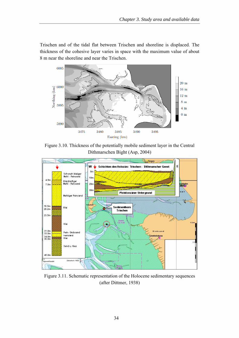
Chapter 3. Study area and available data
Trischen and of the tidal flat between Trischen and shoreline is displaced. The thickness of the cohesive layer varies in space with the maximum value of about 8 m near the shoreline and near the Trischen.
Figure 3.10. Thickness of the potentially mobile sediment layer in the Central Dithmarschen Bight (Asp, 2004)
Figure 3.11. Schematic representation of the Holocene sedimentary sequences (after Dittmer, 1938)
34
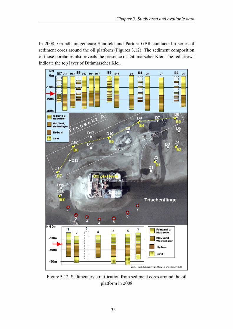
Chapter 3. Study area and available data
In 2008, Grundbauingenieure Steinfeld und Partner GBR conducted a series of sediment cores around the oil platform (Figures 3.12). The sediment composition of those boreholes also reveals the presence of Dithmarscher Klei. The red arrows indicate the top layer of Dithmarscher Klei.
m
Figure 3.12. Sedimentary stratification from sedimplatform in 2008
35
Trischenflinge
Oil platfor
ent cores around the oil
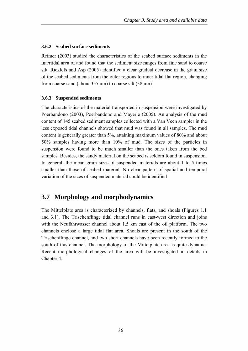
Chapter 3. Study area and available data
3.6.2 Seabed surface sediments
Reimer (2003) studied the characteristics of the seabed surface sediments in the intertidal area of and found that the sediment size ranges from fine sand to coarse silt. Ricklefs and Asp (2005) identified a clear gradual decrease in the grain size of the seabed sediments from the outer regions to inner tidal flat region, changing from coarse sand (about 355 µm) to coarse silt (38 µm).
3.6.3 Suspended sediments
The characteristics of the material transported in suspension were investigated by Poerbandono (2003), Poerbandono and Mayerle (2005). An analysis of the mud content of 145 seabed sediment samples collected with a Van Veen sampler in the less exposed tidal channels showed that mud was found in all samples. The mud content is generally greater than 5%, attaining maximum values of 80% and about 50% samples having more than 10% of mud. The sizes of the particles in suspension were found to be much smaller than the ones taken from the bed samples. Besides, the sandy material on the seabed is seldom found in suspension. In general, the mean grain sizes of suspended materials are about 1 to 5 times smaller than those of seabed material. No clear pattern of spatial and temporal variation of the sizes of suspended material could be identified
3.7 Morphology and morphodynamics
The Mittelplate area is characterized by channels, flats, and shoals (Figures 1.1 and 3.1). The Trischenflinge tidal channel runs in east-west direction and joins with the Neufahrwasser channel about 1.5 km east of the oil platform. The two channels enclose a large tidal flat area. Shoals are present in the south of the Trischenflinge channel, and two short channels have been recently formed to the south of this channel. The morphology of the Mittelplate area is quite dynamic. Recent morphological changes of the area will be investigated in details in Chapter 4.
36
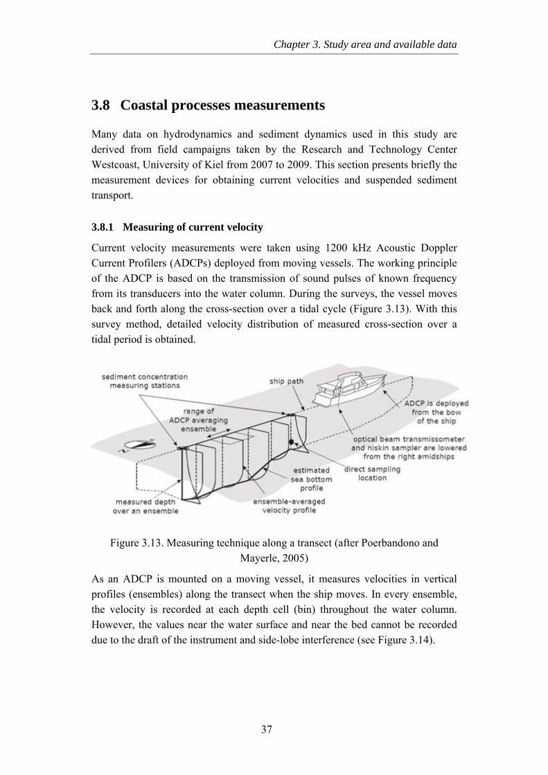
Chapter 3. Study area and available data
3.8 Coastal processes measurements
Many data on hydrodynamics and sediment dynamics used in this study are derived from field campaigns taken by the Research and Technology Center Westcoast, University of Kiel from 2007 to 2009. This section presents briefly the measurement devices for obtaining current velocities and suspended sediment transport.
3.8.1 Measuring of current velocity
Current velocity measurements were taken using 1200 kHz Acoustic Doppler Current Profilers (ADCPs) deployed from moving vessels. The working principle of the ADCP is based on the transmission of sound pulses of known frequency from its transducers into the water column. During the surveys, the vessel moves back and forth along the cross-section over a tidal cycle (Figure 3.13). With this survey method, detailed velocity distribution of measured cross-section over a tidal period is obtained.
Figure 3.13. Measuring technique along a transect (after Poerbandono and Mayerle, 2005)
As an ADCP is mounted on a moving vessel, it measures velocities in vertical profiles (ensembles) along the transect when the ship moves. In every ensemble, the velocity is recorded at each depth cell (bin) throughout the water column. However, the values near the water surface and near the bed cannot be recorded due to the draft of the instrument and side-lobe interference (see Figure 3.14).
37
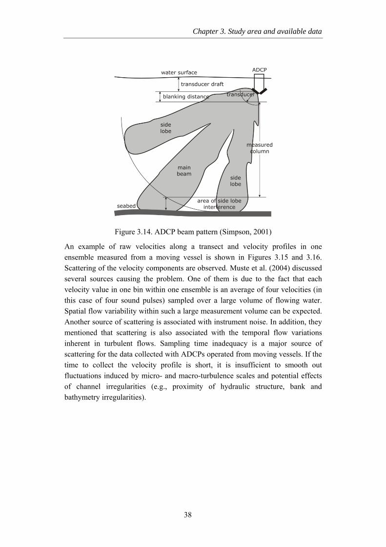
Chapter 3. Study area and available data
Figure 3.14. ADCP beam pattern (Simpson, 2001)
An example of raw velocities along a transect and velocity profiles in one ensemble measured from a moving vessel is shown in Figures 3.15 and 3.16. Scattering of the velocity components are observed. Muste et al. (2004) discussed several sources causing the problem. One of them is due to the fact that each velocity value in one bin within one ensemble is an average of four velocities (in this case of four sound pulses) sampled over a large volume of flowing water. Spatial flow variability within such a large measurement volume can be expected. Another source of scattering is associated with instrument noise. In addition, they mentioned that scattering is also associated with the temporal flow variations inherent in turbulent flows. Sampling time inadequacy is a major source of scattering for the data collected with ADCPs operated from moving vessels. If the time to collect the velocity profile is short, it is insufficient to smooth out fluctuations induced by micro- and macro-turbulence scales and potential effects of channel irregularities (e.g., proximity of hydraulic structure, bank and bathymetry irregularities).
38
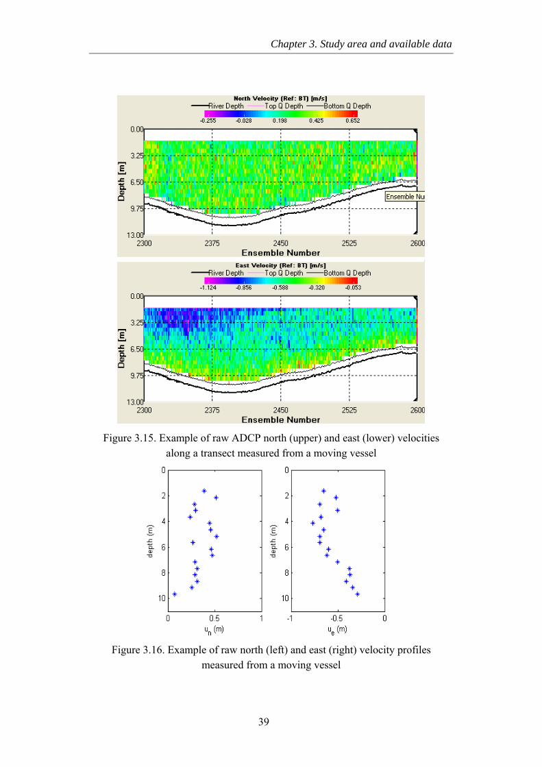
Chapter 3. Study area and available data
Figure 3.15. Example of raw ADCP north (upper) and east (lower) velocities along a transect measured from a moving vessel
Figure 3.16. Example of raw north (left) and east (right) velocity profiles measured from a moving vessel
39

Chapter 3. Study area and available data
3.8.2 Measuring of suspended load
Several techniques have been used to measure suspended sediment basing on mechanical, optical, or acoustical principles. Devices for measuring suspended sediment concentration used in this study base on the first two methods. A measuring system, consisting of an optical beam transmissometer, Conductivity-Temperature-Depth (CTD) sensors, and a trap sampler, is used to provide simultaneous measurement of optical transmission, depth, water properties, and directly sampled sediment concentration. They are all mounted on a frame as shown in Figure 3.17. In each cruise, the frame is lowered at designed vertical stations along measured cross-sections (Figure 3.13).
An optical beam transmissometer consists of a transmitter (light source) and receiver (light detector), separated by a path length L (see Figure 3.17). The transmitter emits a red light beam with 660±12 nm wavelength and the receiver detects how much of that beam is scattered back. The high amount of light lost is associated with large suspended concentrations and vice versa.
Trap sampler is a mechanical device. It has cylinder shape and can collect about 2 litre water samples, which are then filtered for the sediment content.
Optical sampling is indirect technique, which does not provide directly measurement of suspended sediment concentration but percentage of optical transmission. A simultaneous data measured with the trap sampler is used for converting optical transmission measurement to suspended sediment concentration by developing a calibration curve.
An example of a calibration curve is shown in Figure 3.18. The curve is presented in exponent form with the correlation coefficient with the measured data of 0.9.
40
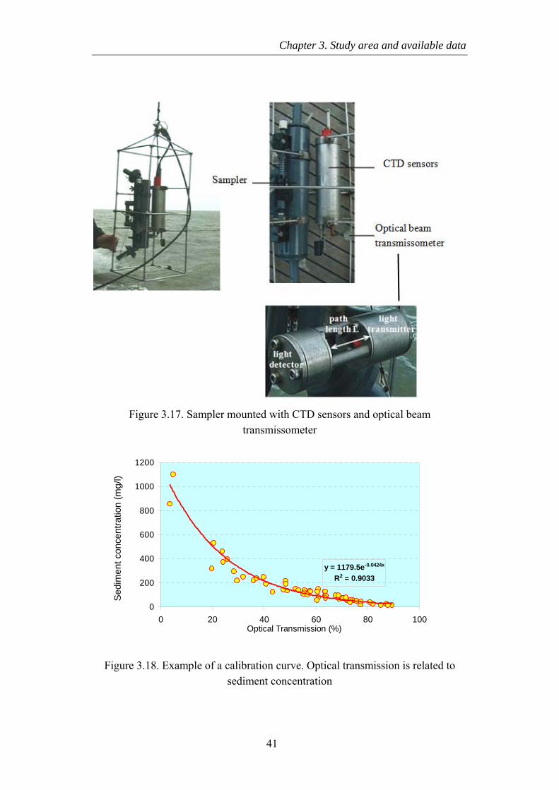
Chapter 3. Study area and available data
Figure 3.17. Sampler mounted with CTD sensors and optical beam transmissometer
y = 1179.5e-0.0424x
R2 = 0.9033
0
200
400
600
800
1000
1200
0 20 40 60 80 100Optical Transmission (%)
Sed
imen
t con
cent
ratio
n (m
g/l))
S
edim
ent c
once
ntra
tion
(mg/
l)
Figure 3.18. Example of a calibration curve. Optical transmission is related to sediment concentration
41
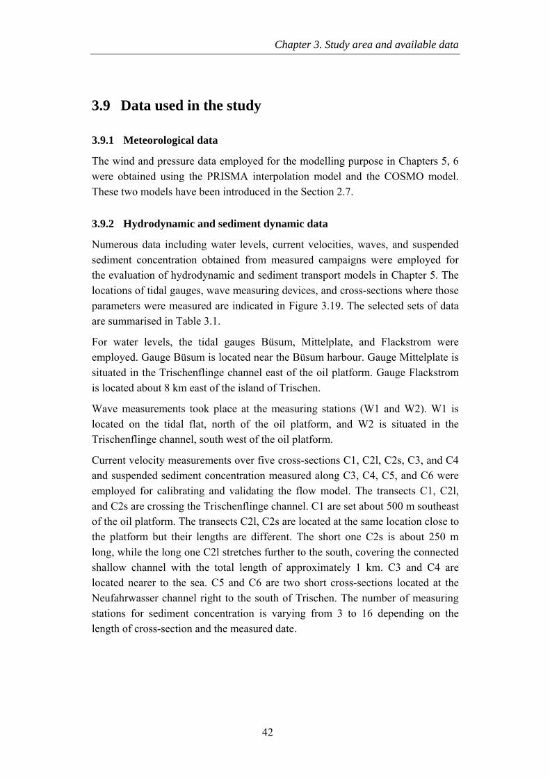
Chapter 3. Study area and available data
3.9 Data used in the study
3.9.1 Meteorological data
The wind and pressure data employed for the modelling purpose in Chapters 5, 6 were obtained using the PRISMA interpolation model and the COSMO model. These two models have been introduced in the Section 2.7.
3.9.2 Hydrodynamic and sediment dynamic data
Numerous data including water levels, current velocities, waves, and suspended sediment concentration obtained from measured campaigns were employed for the evaluation of hydrodynamic and sediment transport models in Chapter 5. The locations of tidal gauges, wave measuring devices, and cross-sections where those parameters were measured are indicated in Figure 3.19. The selected sets of data are summarised in Table 3.1.
For water levels, the tidal gauges Büsum, Mittelplate, and Flackstrom were employed. Gauge Büsum is located near the Büsum harbour. Gauge Mittelplate is situated in the Trischenflinge channel east of the oil platform. Gauge Flackstrom is located about 8 km east of the island of Trischen.
Wave measurements took place at the measuring stations (W1 and W2). W1 is located on the tidal flat, north of the oil platform, and W2 is situated in the Trischenflinge channel, south west of the oil platform.
Current velocity measurements over five cross-sections C1, C2l, C2s, C3, and C4 and suspended sediment concentration measured along C3, C4, C5, and C6 were employed for calibrating and validating the flow model. The transects C1, C2l, and C2s are crossing the Trischenflinge channel. C1 are set about 500 m southeast of the oil platform. The transects C2l, C2s are located at the same location close to the platform but their lengths are different. The short one C2s is about 250 m long, while the long one C2l stretches further to the south, covering the connected shallow channel with the total length of approximately 1 km. C3 and C4 are located nearer to the sea. C5 and C6 are two short cross-sections located at the Neufahrwasser channel right to the south of Trischen. The number of measuring stations for sediment concentration is varying from 3 to 16 depending on the length of cross-section and the measured date.
42
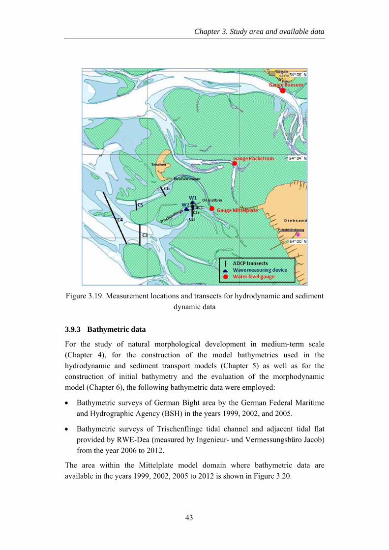
Chapter 3. Study area and available data
Figure 3.19. Measurement locations and transects for hydrodynamic and sediment dynamic data
3.9.3 Bathymetric data
For the study of natural morphological development in medium-term scale (Chapter 4), for the construction of the model bathymetries used in the hydrodynamic and sediment transport models (Chapter 5) as well as for the construction of initial bathymetry and the evaluation of the morphodynamic model (Chapter 6), the following bathymetric data were employed:
• Bathymetric surveys of German Bight area by the German Federal Maritime and Hydrographic Agency (BSH) in the years 1999, 2002, and 2005.
• Bathymetric surveys of Trischenflinge tidal channel and adjacent tidal flat provided by RWE-Dea (measured by Ingenieur- und Vermessungsbüro Jacob) from the year 2006 to 2012.
The area within the Mittelplate model domain where bathymetric data are available in the years 1999, 2002, 2005 to 2012 is shown in Figure 3.20.
43
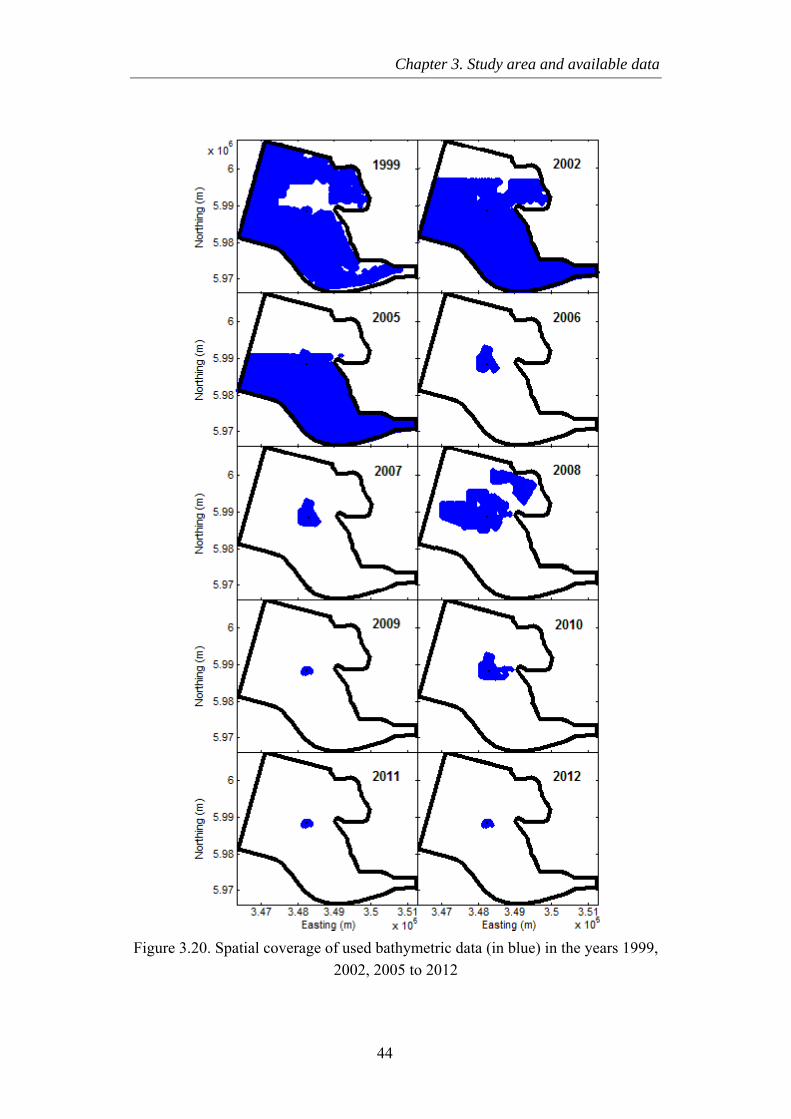
Chapter 3. Study area and available data
Figure 3.20. Spatial coverage of used bathymetric data (in blue) in the years 1999,
2002, 2005 to 2012
44
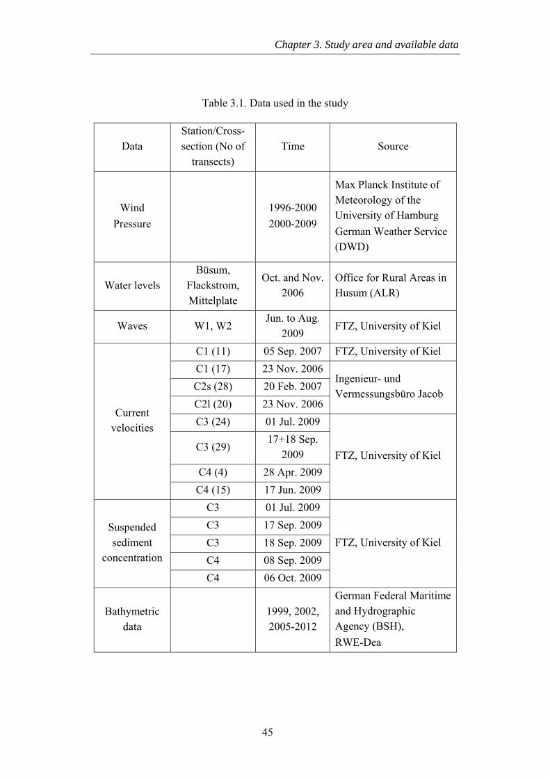
Chapter 3. Study area and available data
Table 3.1. Data used in the study
Data Station/Cross-section (No of
transects) Time Source
Wind Pressure
1996-2000 2000-2009
Max Planck Institute of Meteorology of the University of Hamburg German Weather Service (DWD)
Water levels Büsum,
Flackstrom, Mittelplate
Oct. and Nov. 2006
Office for Rural Areas in Husum (ALR)
Waves W1, W2 Jun. to Aug.
2009 FTZ, University of Kiel
C1 (11) 05 Sep. 2007 FTZ, University of Kiel C1 (17) 23 Nov. 2006 C2s (28) 20 Feb. 2007 C2l (20) 23 Nov. 2006
Ingenieur- und Vermessungsbüro Jacob
C3 (24) 01 Jul. 2009
C3 (29) 17+18 Sep.
2009 C4 (4) 28 Apr. 2009
Current velocities
C4 (15) 17 Jun. 2009
FTZ, University of Kiel
C3 01 Jul. 2009 C3 17 Sep. 2009 C3 18 Sep. 2009 C4 08 Sep. 2009
Suspended sediment
concentration
C4 06 Oct. 2009
FTZ, University of Kiel
Bathymetric data
1999, 2002, 2005-2012
German Federal Maritime and Hydrographic Agency (BSH), RWE-Dea
45

46
Chapter 4
Medium-term morphodynamic evolution of the Mittelplate area - field measurements
4.1 Introduction
Field data of morphological changes in medium- and long-term time scale in the coastal environments including tidal flat areas are generally limited due the difficulty and expense of conducting bathymetric surveys in nearshore zones. To reach the aims of the projects, extensive measurements on hydrodynamics, sediment dynamics, and morphodynamics have been carried out in the study area.
This chapter presents a study of medium-term morphodynamics of the Mittelplate area on the basis of the bathymetric measurements. Morphological changes in the area over six-year period 2006-2012 and possible causes are investigated in details.
4.2 Methods
In order to study the natural development in morphology of the study area, the measured bathymetric data from 2006-2012 provided by the company RWE-Dea were analyzed. Most of the surveyed data (intervals of month to year) covered the
47
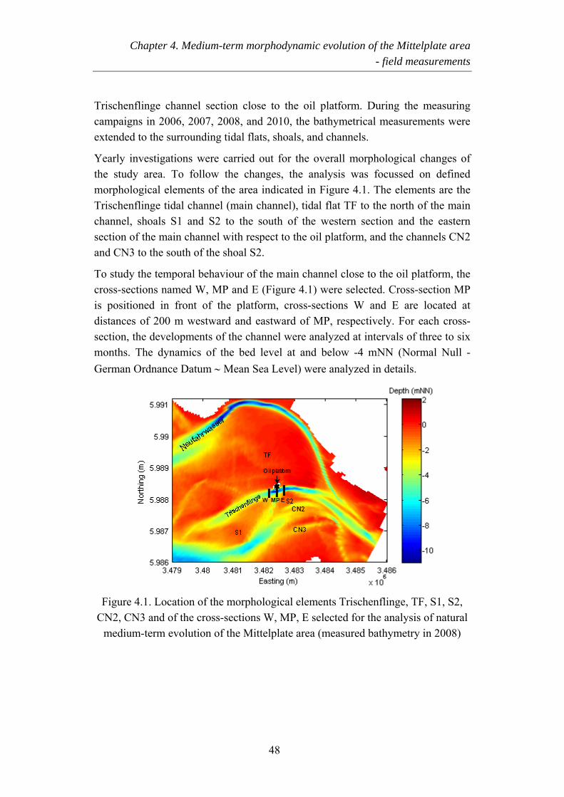
Chapter 4. Medium-term morphodynamic evolution of the Mittelplate area - field measurements
Trischenflinge channel section close to the oil platform. During the measuring campaigns in 2006, 2007, 2008, and 2010, the bathymetrical measurements were extended to the surrounding tidal flats, shoals, and channels.
Yearly investigations were carried out for the overall morphological changes of the study area. To follow the changes, the analysis was focussed on defined morphological elements of the area indicated in Figure 4.1. The elements are the Trischenflinge tidal channel (main channel), tidal flat TF to the north of the main channel, shoals S1 and S2 to the south of the western section and the eastern section of the main channel with respect to the oil platform, and the channels CN2 and CN3 to the south of the shoal S2.
To study the temporal behaviour of the main channel close to the oil platform, the cross-sections named W, MP and E (Figure 4.1) were selected. Cross-section MP is positioned in front of the platform, cross-sections W and E are located at distances of 200 m westward and eastward of MP, respectively. For each cross-section, the developments of the channel were analyzed at intervals of three to six months. The dynamics of the bed level at and below -4 mNN (Normal Null - German Ordnance Datum ∼ Mean Sea Level) were analyzed in details.
Figure 4.1. Location of the morphological elements Trischenflinge, TF, S1, S2, CN2, CN3 and of the cross-sections W, MP, E selected for the analysis of natural
medium-term evolution of the Mittelplate area (measured bathymetry in 2008)
48
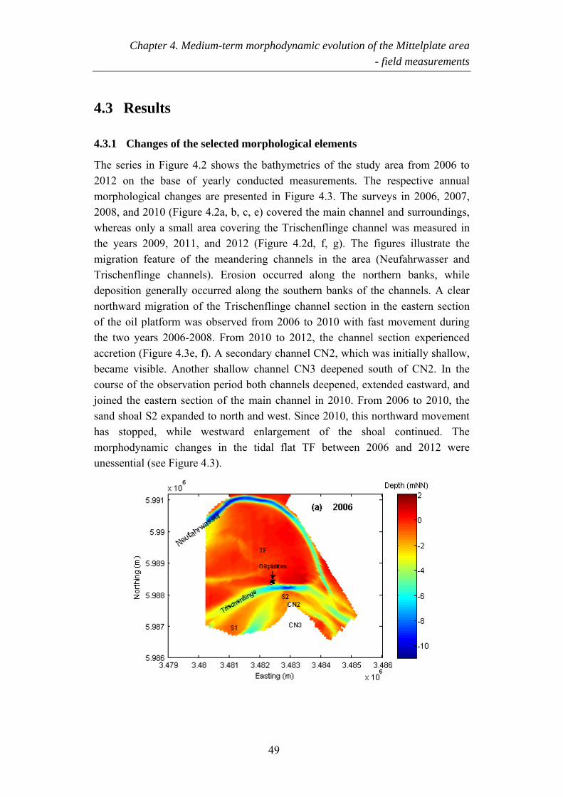
Chapter 4. Medium-term morphodynamic evolution of the Mittelplate area - field measurements
4.3 Results
4.3.1 Changes of the selected morphological elements
The series in Figure 4.2 shows the bathymetries of the study area from 2006 to 2012 on the base of yearly conducted measurements. The respective annual morphological changes are presented in Figure 4.3. The surveys in 2006, 2007, 2008, and 2010 (Figure 4.2a, b, c, e) covered the main channel and surroundings, whereas only a small area covering the Trischenflinge channel was measured in the years 2009, 2011, and 2012 (Figure 4.2d, f, g). The figures illustrate the migration feature of the meandering channels in the area (Neufahrwasser and Trischenflinge channels). Erosion occurred along the northern banks, while deposition generally occurred along the southern banks of the channels. A clear northward migration of the Trischenflinge channel section in the eastern section of the oil platform was observed from 2006 to 2010 with fast movement during the two years 2006-2008. From 2010 to 2012, the channel section experienced accretion (Figure 4.3e, f). A secondary channel CN2, which was initially shallow, became visible. Another shallow channel CN3 deepened south of CN2. In the course of the observation period both channels deepened, extended eastward, and joined the eastern section of the main channel in 2010. From 2006 to 2010, the sand shoal S2 expanded to north and west. Since 2010, this northward movement has stopped, while westward enlargement of the shoal continued. The morphodynamic changes in the tidal flat TF between 2006 and 2012 were unessential (see Figure 4.3).
49
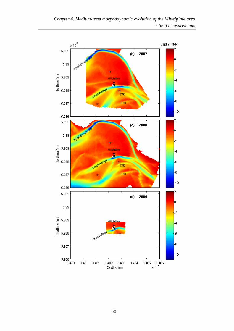
Chapter 4. Medium-term morphodynamic evolution of the Mittelplate area - field measurements
50
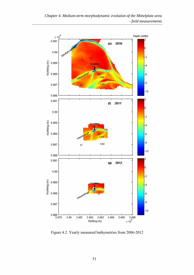
Chapter 4. Medium-term morphodynamic evolution of the Mittelplate area - field measurements
Figure 4.2. Yearly measured bathymetries from 2006-2012
51
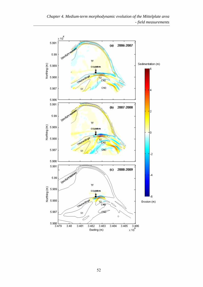
Chapter 4. Medium-term morphodynamic evolution of the Mittelplate area - field measurements
52
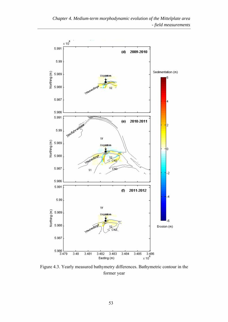
Chapter 4. Medium-term morphodynamic evolution of the Mittelplate area - field measurements
Figure 4.3. Yearly measured bathymetry differences. Bathymetric contour in the former year
53
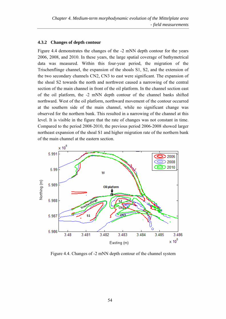
Chapter 4. Medium-term morphodynamic evolution of the Mittelplate area - field measurements
4.3.2 Changes of depth contour
Figure 4.4 demonstrates the changes of the -2 mNN depth contour for the years 2006, 2008, and 2010. In these years, the large spatial coverage of bathymetrical data was measured. Within this four-year period, the migration of the Trischenflinge channel, the expansion of the shoals S1, S2, and the extension of the two secondary channels CN2, CN3 to east were significant. The expansion of the shoal S2 towards the north and northwest caused a narrowing of the central section of the main channel in front of the oil platform. In the channel section east of the oil platform, the -2 mNN depth contour of the channel banks shifted northward. West of the oil platform, northward movement of the contour occurred at the southern side of the main channel, while no significant change was observed for the northern bank. This resulted in a narrowing of the channel at this level. It is visible in the figure that the rate of changes was not constant in time. Compared to the period 2008-2010, the previous period 2006-2008 showed larger northeast expansion of the shoal S1 and higher migration rate of the northern bank of the main channel at the eastern section.
Figure 4.4. Changes of -2 mNN depth contour of the channel system
54
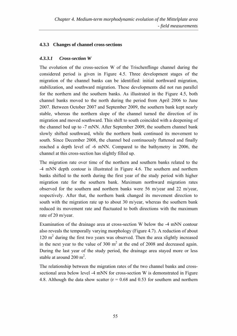
Chapter 4. Medium-term morphodynamic evolution of the Mittelplate area - field measurements
4.3.3 Changes of channel cross-sections
4.3.3.1 Cross-section W
The evolution of the cross-section W of the Trischenflinge channel during the considered period is given in Figure 4.5. Three development stages of the migration of the channel banks can be identified: initial northward migration, stabilization, and southward migration. These developments did not run parallel for the northern and the southern banks. As illustrated in the Figure 4.5, both channel banks moved to the north during the period from April 2006 to June 2007. Between October 2007 and September 2009, the southern bank kept nearly stable, whereas the northern slope of the channel turned the direction of its migration and moved southward. This shift to south coincided with a deepening of the channel bed up to -7 mNN. After September 2009, the southern channel bank slowly shifted southward, while the northern bank continued its movement to south. Since December 2008, the channel bed continuously flattened and finally reached a depth level of -6 mNN. Compared to the bathymetry in 2006, the channel at this cross-section has slightly filled up.
The migration rate over time of the northern and southern banks related to the -4 mNN depth contour is illustrated in Figure 4.6. The southern and northern banks shifted to the north during the first year of the study period with higher migration rate for the southern bank. Maximum northward migration rates observed for the southern and northern banks were 56 m/year and 22 m/year, respectively. After that, the northern bank changed its movement direction to south with the migration rate up to about 30 m/year, whereas the southern bank reduced its movement rate and fluctuated to both directions with the maximum rate of 20 m/year.
Examination of the drainage area at cross-section W below the -4 mNN contour also reveals the temporally varying morphology (Figure 4.7). A reduction of about 120 m2 during the first two years was observed. Then the area slightly increased in the next year to the value of 300 m2 at the end of 2008 and decreased again. During the last year of the study period, the drainage area stayed more or less stable at around 200 m2.
The relationship between the migration rates of the two channel banks and cross-sectional area below level -4 mNN for cross-section W is demonstrated in Figure 4.8. Although the data show scatter (r = 0.68 and 0.53 for southern and northern
55
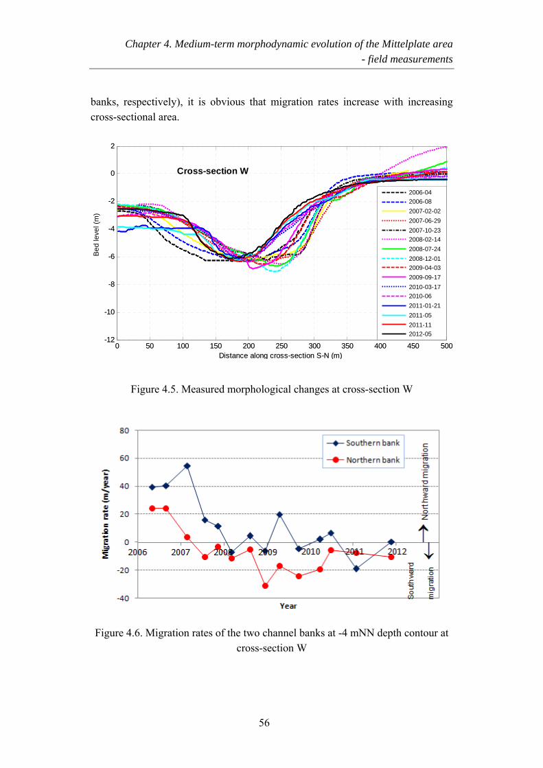
Chapter 4. Medium-term morphodynamic evolution of the Mittelplate area - field measurements
banks, respectively), it is obvious that migration rates increase with increasing cross-sectional area.
0 50 100 150 200 250 300 350 400 450 500-12
-10
-8
-6
-4
-2
0
2
Distance along cross-section S-N (m)
Bedlevel(m)
Cross-section W
0 50 100 150 200 250 300 350 400 450 500-12
-10
-8
-6
-4
-2
0
2
Distance along cross-section S-N (m)
Bedlevel(m)
Bed
leve
l (m
)
2006-042006-082007-02-022007-06-292007-10-232008-02-142008-07-242008-12-012009-04-032009-09-172010-03-172010-062011-01-212011-052011-112012-05
Figure 4.5. Measured morphological changes at cross-section W
Figure 4.6. Migration rates of the two channel banks at -4 mNN depth contour at cross-section W
56
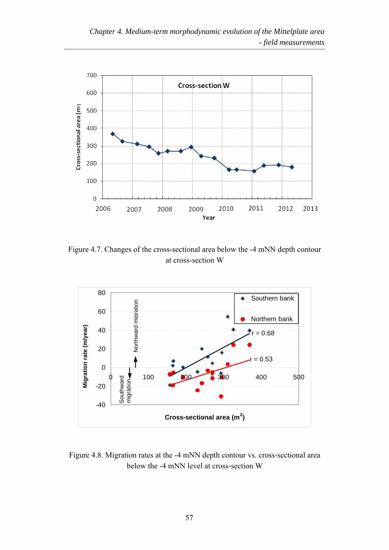
Chapter 4. Medium-term morphodynamic evolution of the Mittelplate area - field measurements
Figure 4.7. Changes of the cross-sectional area below the -4 mNN depth contour at cross-section W
r = 0.68
r = 0.53
-40
-20
0
20
40
60
80
0 100 200 300 400 500
Cross-sectional area (m2)
Southern bank
Northern bank
Nor
thw
ard
mig
ratio
n
Mig
ratio
n ra
te (m
/yea
r)
Sou
thw
ard
mig
ratio
n
Figure 4.8. Migration rates at the -4 mNN depth contour vs. cross-sectional area below the -4 mNN level at cross-section W
57
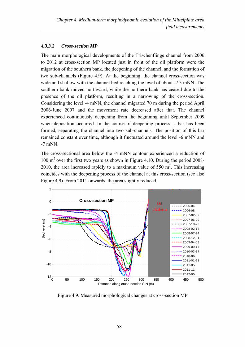
Chapter 4. Medium-term morphodynamic evolution of the Mittelplate area - field measurements
4.3.3.2 Cross-section MP
The main morphological developments of the Trischenflinge channel from 2006 to 2012 at cross-section MP located just in front of the oil platform were the migration of the southern bank, the deepening of the channel, and the formation of two sub-channels (Figure 4.9). At the beginning, the channel cross-section was wide and shallow with the channel bed reaching the level of about -7.3 mNN. The southern bank moved northward, while the northern bank has ceased due to the presence of the oil platform, resulting in a narrowing of the cross-section. Considering the level -4 mNN, the channel migrated 70 m during the period April 2006-June 2007 and the movement rate decreased after that. The channel experienced continuously deepening from the beginning until September 2009 when deposition occurred. In the course of deepening process, a bar has been formed, separating the channel into two sub-channels. The position of this bar remained constant over time, although it fluctuated around the level -6 mNN and -7 mNN.
The cross-sectional area below the -4 mNN contour experienced a reduction of 100 m2 over the first two years as shown in Figure 4.10. During the period 2008-2010, the area increased rapidly to a maximum value of 550 m2. This increasing coincides with the deepening process of the channel at this cross-section (see also Figure 4.9). From 2011 onwards, the area slightly reduced.
0 50 100 150 200 250 300 350 400 450 500-12
-10
-8
-6
-4
-2
0
2
Distance along cross-section S-N (m)
Beevem
Cross-section MP
0 50 100 150 200 250 300 350 400 450 500-12
-10
-8
-6
-4
-2
0
2
Distance along cross-section S-N (m)
Beevem
2006-042006-082007-02-022007-06-292007-10-232008-02-142008-07-242008-12-012009-04-032009-09-172010-03-172010-062011-01-212011-052011-112012-05
Oil platform
Bed
el
(m)
lev
Figure 4.9. Measured morphological changes at cross-section MP
58
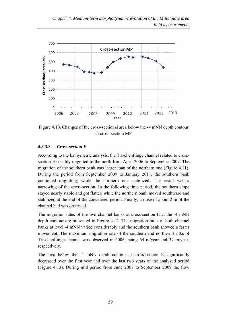
Chapter 4. Medium-term morphodynamic evolution of the Mittelplate area - field measurements
Figure 4.10. Changes of the cross-sectional area below the -4 mNN depth contour at cross-section MP
4.3.3.3 Cross-section E
According to the bathymetric analysis, the Trischenflinge channel related to cross-section E steadily migrated to the north from April 2006 to September 2009. The migration of the southern bank was larger than of the northern one (Figure 4.11). During the period from September 2009 to January 2011, the southern bank continued migrating, while the northern one stabilized. The result was a narrowing of the cross-section. In the following time period, the southern slope stayed nearly stable and got flatter, while the northern bank moved southward and stabilized at the end of the considered period. Finally, a raise of about 2 m of the channel bed was observed.
The migration rates of the two channel banks at cross-section E at the -4 mNN depth contour are presented in Figure 4.12. The migration rates of both channel banks at level -4 mNN varied considerably and the southern bank showed a faster movement. The maximum migration rate of the southern and northern banks of Trischenflinge channel was observed in 2006, being 64 m/year and 37 m/year, respectively.
The area below the -4 mNN depth contour at cross-section E significantly decreased over the first year and over the last two years of the analyzed period (Figure 4.13). During mid period from June 2007 to September 2009 the flow
59
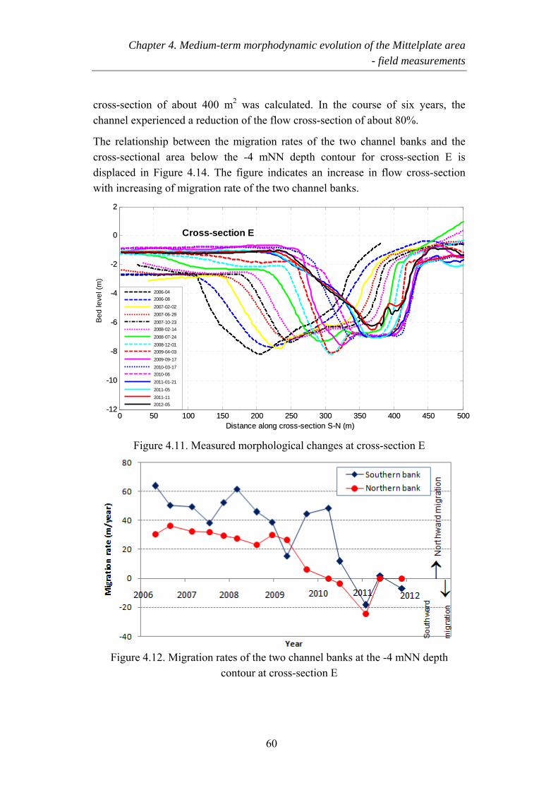
Chapter 4. Medium-term morphodynamic evolution of the Mittelplate area - field measurements
cross-section of about 400 m2 was calculated. In the course of six years, the channel experienced a reduction of the flow cross-section of about 80%.
The relationship between the migration rates of the two channel banks and the cross-sectional area below the -4 mNN depth contour for cross-section E is displaced in Figure 4.14. The figure indicates an increase in flow cross-section with increasing of migration rate of the two channel banks.
0 50 100 150 200 250 300 350 400 450 500-12
-10
-8
-6
-4
-2
0
2
Distance along cross-section S-N (m)
Bedlevel(m)
Cross-section E
0 50 100 150 200 250 300 350 400 450 500
-12
-10
-8
-6
-4
-2
0
2
Distance along cross-section S-N (m)
Bedlevel(m) 2006-04
2006-082007-02-022007-06-292007-10-232008-02-142008-07-242008-12-012009-04-032009-09-172010-03-172010-062011-01-212011-052011-112012-05
Bed
leve
l (m
)
Figure 4.11. Measured morphological changes at cross-section E
Figure 4.12. Migration rates of the two channel banks at the -4 mNN depth
contour at cross-section E
60
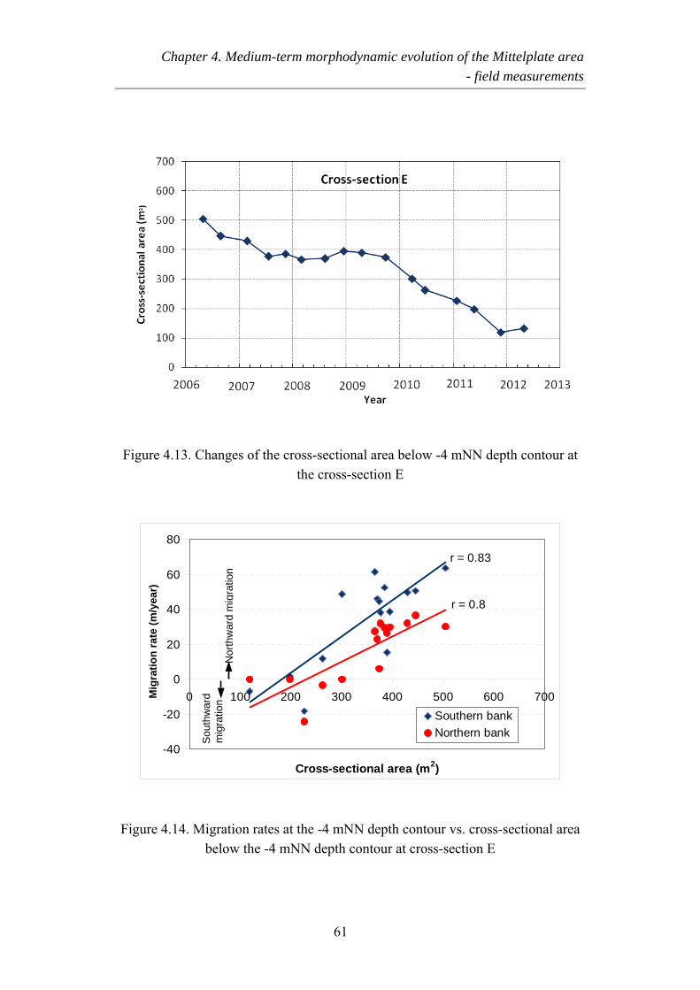
Chapter 4. Medium-term morphodynamic evolution of the Mittelplate area - field measurements
Figure 4.13. Changes of the cross-sectional area below -4 mNN depth contour at the cross-section E
r = 0.83
r = 0.8
-40
-20
0
20
40
60
80
0 100 200 300 400 500 600 700
Cross-sectional area (m2)
Southern bankNorthern bank
Nor
thw
ard
mig
ratio
n
Sou
thw
ard
mig
ratio
n Mig
ratio
n ra
te (m
/yea
r)
Figure 4.14. Migration rates at the -4 mNN depth contour vs. cross-sectional area below the -4 mNN depth contour at cross-section E
61
Chapter 4. Medium-term morphodynamic evolution of the Mittelplate area - field measurements
4.4 Discussion
On the basis of high-resolution bathymetric measurements, the morphological developments of the Trischenflinge tidal channel and adjacent coastal area were investigated. The analysis of the data over the period of six years from April 2006 till May 2012 revealed the strong dynamics of the system. The most obvious changes were the migration of the Trischenflinge tidal channel, the deepening of the channel section in front of the oil platform, the expansion and the migration of the shoals, the formation, the deepening and the breaking through of the channels CN2, CN3. Within the considered period, the first two years 2006-2008 showed the most morphological changes with rapid migration of the eastern section of the main channel, large expansion the shoal S1 to the northeast direction.
Analysis of the three individual cross-sections within the Trischenflinge channel located 200 m apart over the six-year period revealed considerable spatial and temporal variability in the morphodynamic response of the channel. The cross-section E showed strongest northward movement with the maximum rate at the beginning of the period of 64 m/year and 37 m/year for the southern and northern banks, respectively. At cross-section MP, the northern bank of the channel has ceased due to the presence of a scour protection in front of the oil platform, while the southern bank moved northward, causing the channel deepening up to about 5 m during the considered period. For cross-sections W and E with the two channel banks experiencing migration, the migration rates of the both banks were found to increase with increasing of the cross-sectional area below the level -4 mNN.
Overall, the cross-sectional area below the -4 mNN depth contour at cross-sections W and E decreased over the six-year period with the largest reduction of about 80% for the cross-section E. This indicates that the role of the Trischenflinge as a main drainage channel was decreasing in the course of time.
There was a fluctuation of the channel bed between the level -6 mNN and -8 mNN at the two cross-sections W and E during the six years. In addition, the bar formed in the middle of the channel at cross-section MP fluctuated around the level of -6 mNN to -7 mNN. The cease of the deepening of the channel is a sign for the presence of a consolidated cohesive layer, which is hard to erode as discussed in Chapter 3. The hindrance of channel deepening due to this layer together with the northward migration and expansion of the shoals at the southern channel bank may lead to erosion of the northern bank to maintain the flow cross-section. These processes result in the lateral migration of the main channel.
62
Chapter 4. Medium-term morphodynamic evolution of the Mittelplate area - field measurements
Simultaneous changes were observed at the three examined cross-sections after September 2009. The southward movement of the northern bank of cross-section W was slower. Cross-section MP stopped deepening and got shallower. For the cross-section E, the northern bank did not move to north any more, but became stable or moved southward. In addition, the last two years of the study period showed sedimentation feature of the eastern section of the main channel. These may be a consequence of the complete formation of channel network including CN2, CN3 south of the main channel as shown in the measured bathymetry for the year 2010 (Figure 4.2e). These two channels shared the role with the main channel in transporting water from the tidal eastern drainage area to the open North Sea. Moreover, they prevented the material supply from the south to the shoal S2, causing the reduction in pressure on the southern side of the main channel.
63

Chapter 4. Medium-term morphodynamic evolution of the Mittelplate area - field measurements
64
Chapter 5
The Mittelplate models
5.1 Introduction
In this chapter, the development, calibration and validation of the numerical models for simulating flow, waves and sediment transport of the Mittelplate area are presented. The set-up of morphodynamic model, which will be used to study the medium-term morphodynamics of the study area in Chapter 6, is then included. The models have been set-up with the depth-averaged version of Delft3D modelling system. Description of the Delft3D model can be found in Lesser et al. (2004) or Deltares (2008a, b) and is briefly introduced in Section 2.5.
5.1.1 Model domain
The study concerns Mittelplate area, characterised by meandering tidal channels and adjacent tidal flats with the central focus on the Trischenflinge channel and surroundings. An oil platform is present on a tidal flat right to the most northern extension of the Trischenflinge channel. The model domain includes those elements and is extended in all directions in order to ensure a proper representation of the hydrodynamics and morphodynamics in this area (Figure 5.1). The whole domain covers an area of about 940 km2. The eastern side is the coastline and is therefore a closed boundary. The western side forms the link between the model domain and the open North Sea. To the north, the domain covers the Piep channel system. Part of the Elbe river in the southeast is also included.
65
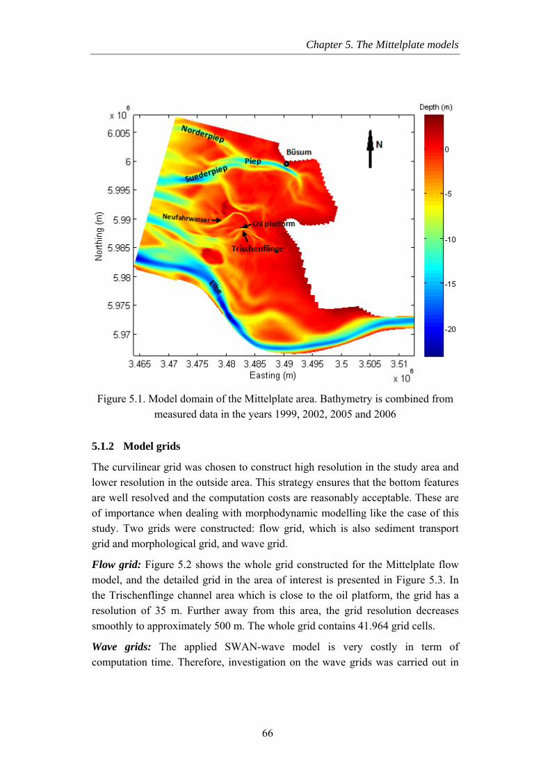
Chapter 5. The Mittelplate models
Figure 5.1. Model domain of the Mittelplate area. Bathymetry is combined from measured data in the years 1999, 2002, 2005 and 2006
5.1.2 Model grids
The curvilinear grid was chosen to construct high resolution in the study area and lower resolution in the outside area. This strategy ensures that the bottom features are well resolved and the computation costs are reasonably acceptable. These are of importance when dealing with morphodynamic modelling like the case of this study. Two grids were constructed: flow grid, which is also sediment transport grid and morphological grid, and wave grid.
Flow grid: Figure 5.2 shows the whole grid constructed for the Mittelplate flow model, and the detailed grid in the area of interest is presented in Figure 5.3. In the Trischenflinge channel area which is close to the oil platform, the grid has a resolution of 35 m. Further away from this area, the grid resolution decreases smoothly to approximately 500 m. The whole grid contains 41.964 grid cells.
Wave grids: The applied SWAN-wave model is very costly in term of computation time. Therefore, investigation on the wave grids was carried out in
66
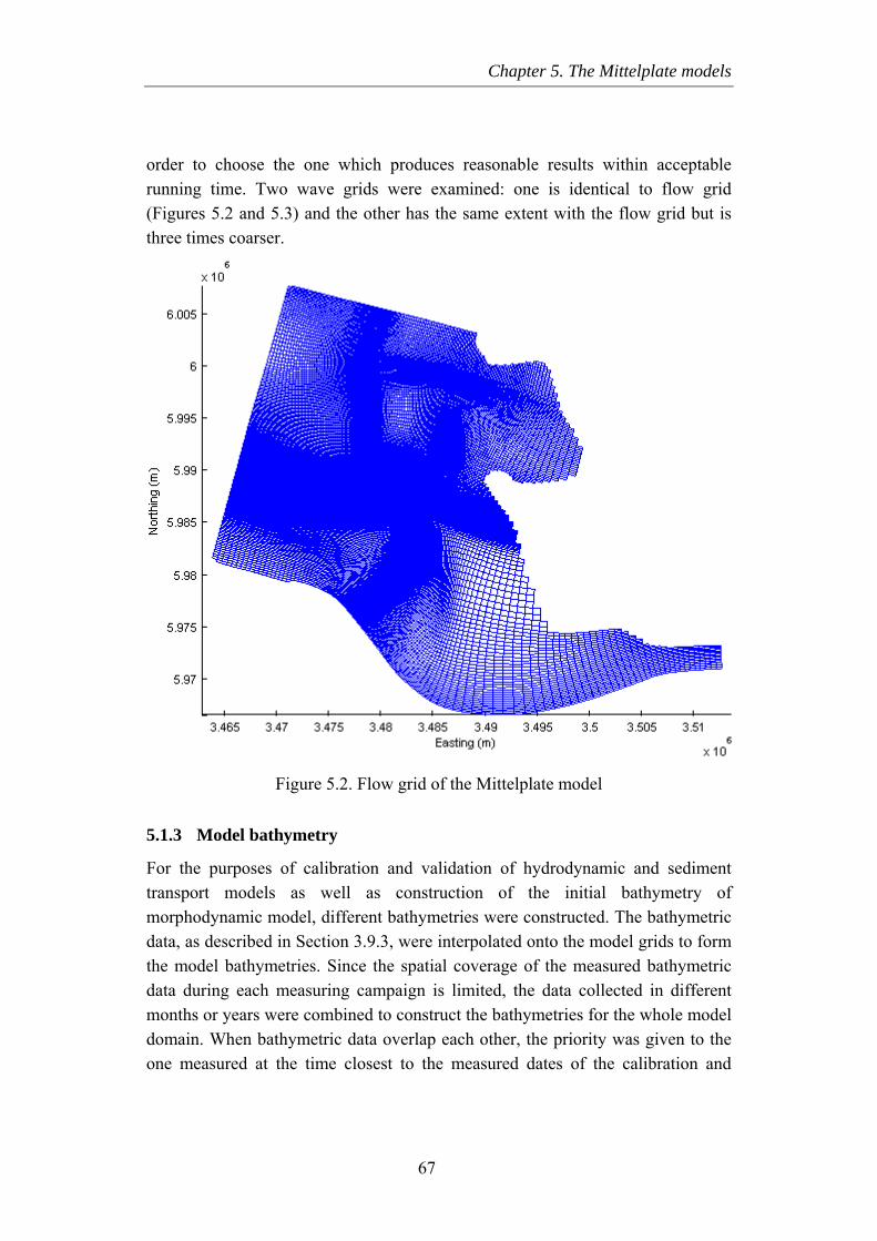
Chapter 5. The Mittelplate models
order to choose the one which produces reasonable results within acceptable running time. Two wave grids were examined: one is identical to flow grid (Figures 5.2 and 5.3) and the other has the same extent with the flow grid but is three times coarser.
Figure 5.2. Flow grid of the Mittelplate model
5.1.3 Model bathymetry
For the purposes of calibration and validation of hydrodynamic and sediment transport models as well as construction of the initial bathymetry of morphodynamic model, different bathymetries were constructed. The bathymetric data, as described in Section 3.9.3, were interpolated onto the model grids to form the model bathymetries. Since the spatial coverage of the measured bathymetric data during each measuring campaign is limited, the data collected in different months or years were combined to construct the bathymetries for the whole model domain. When bathymetric data overlap each other, the priority was given to the one measured at the time closest to the measured dates of the calibration and
67
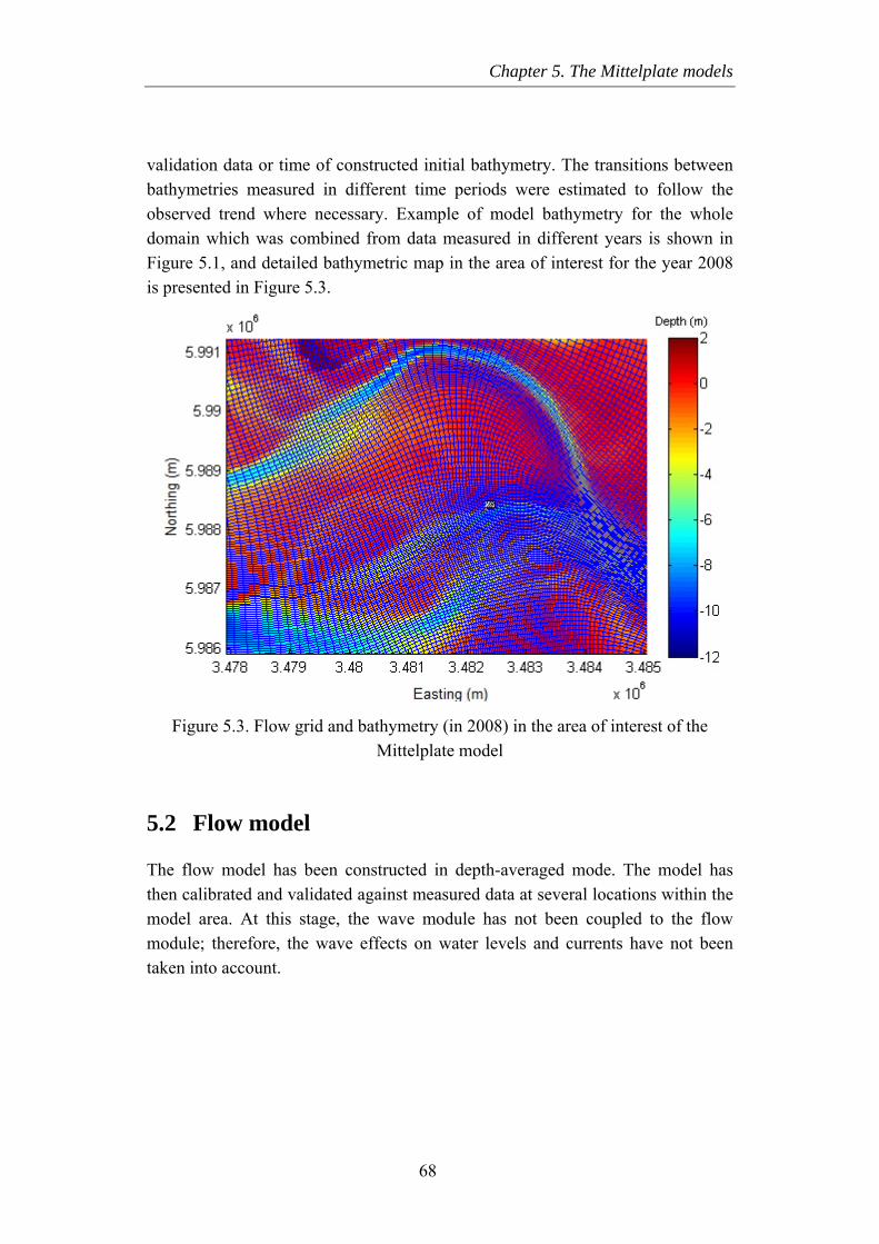
Chapter 5. The Mittelplate models
validation data or time of constructed initial bathymetry. The transitions between bathymetries measured in different time periods were estimated to follow the observed trend where necessary. Example of model bathymetry for the whole domain which was combined from data measured in different years is shown in Figure 5.1, and detailed bathymetric map in the area of interest for the year 2008 is presented in Figure 5.3.
Figure 5.3. Flow grid and bathymetry (in 2008) in the area of interest of the Mittelplate model
5.2 Flow model
The flow model has been constructed in depth-averaged mode. The model has then calibrated and validated against measured data at several locations within the model area. At this stage, the wave module has not been coupled to the flow module; therefore, the wave effects on water levels and currents have not been taken into account.
68
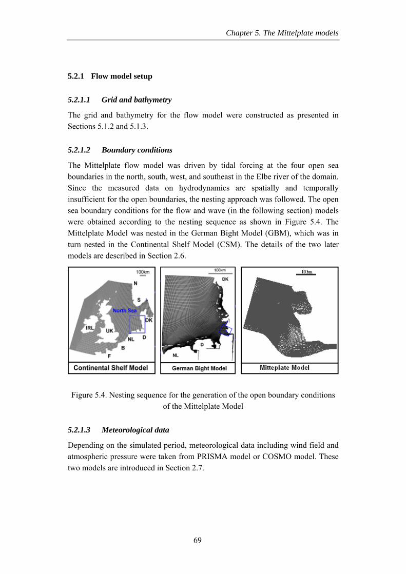
Chapter 5. The Mittelplate models
5.2.1 Flow model setup
5.2.1.1 Grid and bathymetry
The grid and bathymetry for the flow model were constructed as presented in Sections 5.1.2 and 5.1.3.
5.2.1.2 Boundary conditions
The Mittelplate flow model was driven by tidal forcing at the four open sea boundaries in the north, south, west, and southeast in the Elbe river of the domain. Since the measured data on hydrodynamics are spatially and temporally insufficient for the open boundaries, the nesting approach was followed. The open sea boundary conditions for the flow and wave (in the following section) models were obtained according to the nesting sequence as shown in Figure 5.4. The Mittelplate Model was nested in the German Bight Model (GBM), which was in turn nested in the Continental Shelf Model (CSM). The details of the two later models are described in Section 2.6.
Figure 5.4. Nesting sequence for the generation of the open boundary conditions of the Mittelplate Model
5.2.1.3 Meteorological data
Depending on the simulated period, meteorological data including wind field and atmospheric pressure were taken from PRISMA model or COSMO model. These two models are introduced in Section 2.7.
69
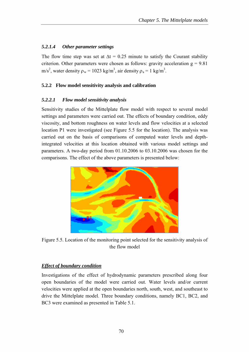
Chapter 5. The Mittelplate models
5.2.1.4 Other parameter settings
The flow time step was set at ∆t = 0.25 minute to satisfy the Courant stability criterion. Other parameters were chosen as follows: gravity acceleration g = 9.81 m/s2, water density ρw = 1023 kg/m3, air density ρa = 1 kg/m3.
5.2.2 Flow model sensitivity analysis and calibration
5.2.2.1 Flow model sensitivity analysis
Sensitivity studies of the Mittelplate flow model with respect to several model settings and parameters were carried out. The effects of boundary condition, eddy viscosity, and bottom roughness on water levels and flow velocities at a selected location P1 were investigated (see Figure 5.5 for the location). The analysis was carried out on the basis of comparisons of computed water levels and depth-integrated velocities at this location obtained with various model settings and parameters. A two-day period from 01.10.2006 to 03.10.2006 was chosen for the comparisons. The effect of the above parameters is presented below:
P1
Figure 5.5. Location of the monitoring point selected for the sensitivity analysis of the flow model
Effect of boundary condition
Investigations of the effect of hydrodynamic parameters prescribed along four open boundaries of the model were carried out. Water levels and/or current velocities were applied at the open boundaries north, south, west, and southeast to drive the Mittelplate model. Three boundary conditions, namely BC1, BC2, and BC3 were examined as presented in Table 5.1.
70
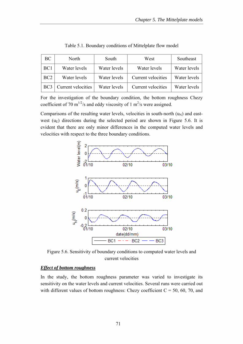
Chapter 5. The Mittelplate models
Table 5.1. Boundary conditions of Mittelplate flow model
BC North South West Southeast
BC1 Water levels Water levels Water levels Water levels
BC2 Water levels Water levels Current velocities Water levels
BC3 Current velocities Water levels Current velocities Water levels
For the investigation of the boundary condition, the bottom roughness Chezy coefficient of 70 m1/2/s and eddy viscosity of 1 m2/s were assigned.
Comparisons of the resulting water levels, velocities in south-north (uN) and east-west (uE) directions during the selected period are shown in Figure 5.6. It is evident that there are only minor differences in the computed water levels and velocities with respect to the three boundary conditions.
Figure 5.6. Sensitivity of boundary conditions to computed water levels and current velocities
Effect of bottom roughness
In the study, the bottom roughness parameter was varied to investigate its sensitivity on the water levels and current velocities. Several runs were carried out with different values of bottom roughness: Chezy coefficient C = 50, 60, 70, and
71
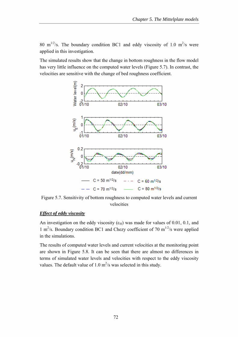
Chapter 5. The Mittelplate models
80 m1/2/s. The boundary condition BC1 and eddy viscosity of 1.0 m2/s were applied in this investigation.
The simulated results show that the change in bottom roughness in the flow model has very little influence on the computed water levels (Figure 5.7). In contrast, the velocities are sensitive with the change of bed roughness coefficient.
Figure 5.7. Sensitivity of bottom roughness to computed water levels and current velocities
Effect of eddy viscosity
An investigation on the eddy viscosity (εH) was made for values of 0.01, 0.1, and 1 m2/s. Boundary condition BC1 and Chezy coefficient of 70 m1/2/s were applied in the simulations.
The results of computed water levels and current velocities at the monitoring point are shown in Figure 5.8. It can be seen that there are almost no differences in terms of simulated water levels and velocities with respect to the eddy viscosity values. The default value of 1.0 m2/s was selected in this study.
72
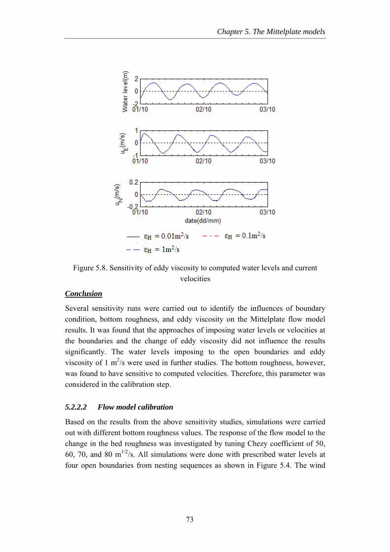
Chapter 5. The Mittelplate models
Figure 5.8. Sensitivity of eddy viscosity to computed water levels and current velocities
Conclusion
Several sensitivity runs were carried out to identify the influences of boundary condition, bottom roughness, and eddy viscosity on the Mittelplate flow model results. It was found that the approaches of imposing water levels or velocities at the boundaries and the change of eddy viscosity did not influence the results significantly. The water levels imposing to the open boundaries and eddy viscosity of 1 m2/s were used in further studies. The bottom roughness, however, was found to have sensitive to computed velocities. Therefore, this parameter was considered in the calibration step.
5.2.2.2 Flow model calibration
Based on the results from the above sensitivity studies, simulations were carried out with different bottom roughness values. The response of the flow model to the change in the bed roughness was investigated by tuning Chezy coefficient of 50, 60, 70, and 80 m1/2/s. All simulations were done with prescribed water levels at four open boundaries from nesting sequences as shown in Figure 5.4. The wind
73
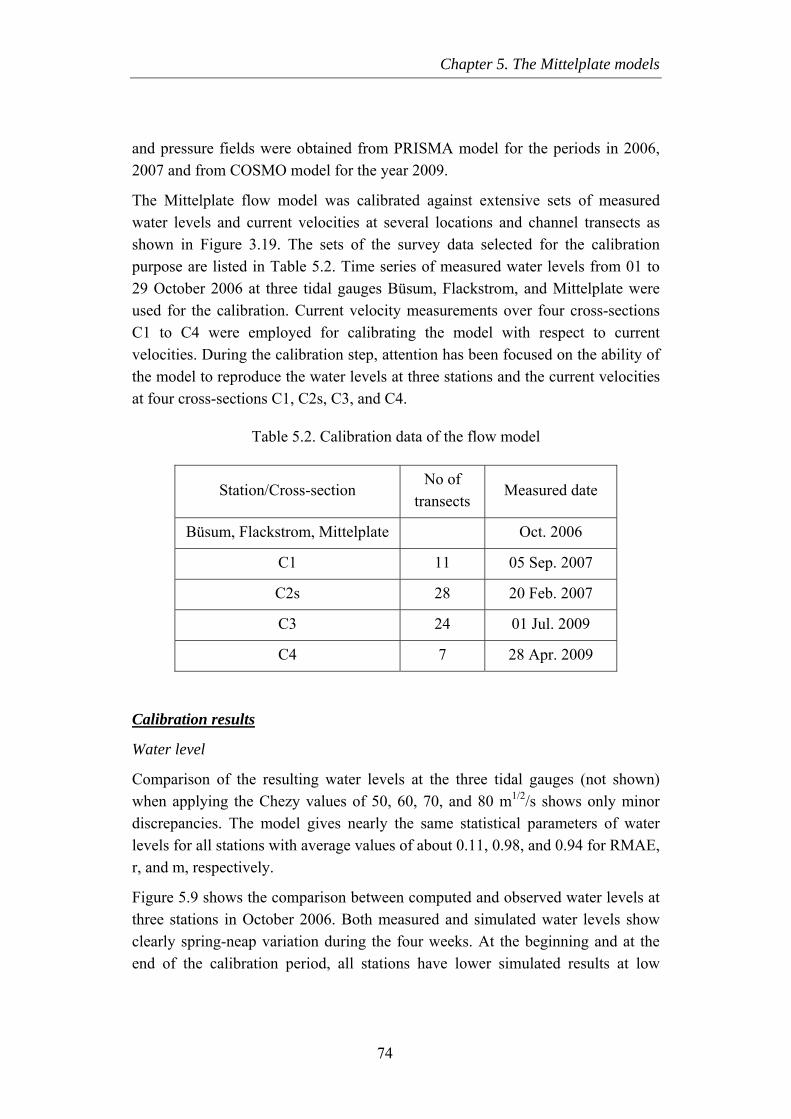
Chapter 5. The Mittelplate models
and pressure fields were obtained from PRISMA model for the periods in 2006, 2007 and from COSMO model for the year 2009.
The Mittelplate flow model was calibrated against extensive sets of measured water levels and current velocities at several locations and channel transects as shown in Figure 3.19. The sets of the survey data selected for the calibration purpose are listed in Table 5.2. Time series of measured water levels from 01 to 29 October 2006 at three tidal gauges Büsum, Flackstrom, and Mittelplate were used for the calibration. Current velocity measurements over four cross-sections C1 to C4 were employed for calibrating the model with respect to current velocities. During the calibration step, attention has been focused on the ability of the model to reproduce the water levels at three stations and the current velocities at four cross-sections C1, C2s, C3, and C4.
Table 5.2. Calibration data of the flow model
Station/Cross-section No of
transects Measured date
Büsum, Flackstrom, Mittelplate Oct. 2006
C1 11 05 Sep. 2007
C2s 28 20 Feb. 2007
C3 24 01 Jul. 2009
C4 7 28 Apr. 2009
Calibration results
Water level
Comparison of the resulting water levels at the three tidal gauges (not shown) when applying the Chezy values of 50, 60, 70, and 80 m1/2/s shows only minor discrepancies. The model gives nearly the same statistical parameters of water levels for all stations with average values of about 0.11, 0.98, and 0.94 for RMAE, r, and m, respectively.
Figure 5.9 shows the comparison between computed and observed water levels at three stations in October 2006. Both measured and simulated water levels show clearly spring-neap variation during the four weeks. At the beginning and at the end of the calibration period, all stations have lower simulated results at low
74
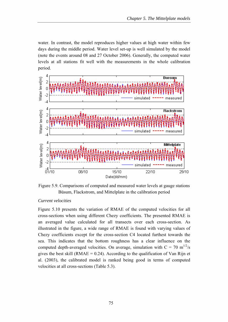
Chapter 5. The Mittelplate models
water. In contrast, the model reproduces higher values at high water within few days during the middle period. Water level set-up is well simulated by the model (note the events around 08 and 27 October 2006). Generally, the computed water levels at all stations fit well with the measurements in the whole calibration period.
Figure 5.9. Comparisons of computed and measured water levels at gauge stations Büsum, Flackstrom, and Mittelplate in the calibration period
Current velocities
Figure 5.10 presents the variation of RMAE of the computed velocities for all cross-sections when using different Chezy coefficients. The presented RMAE is an averaged value calculated for all transects over each cross-section. As illustrated in the figure, a wide range of RMAE is found with varying values of Chezy coefficients except for the cross-section C4 located furthest towards the sea. This indicates that the bottom roughness has a clear influence on the computed depth-averaged velocities. On average, simulation with C = 70 m1/2/s gives the best skill (RMAE = 0.24). According to the qualification of Van Rijn et al. (2003), the calibrated model is ranked being good in terms of computed velocities at all cross-sections (Table 5.3).
75
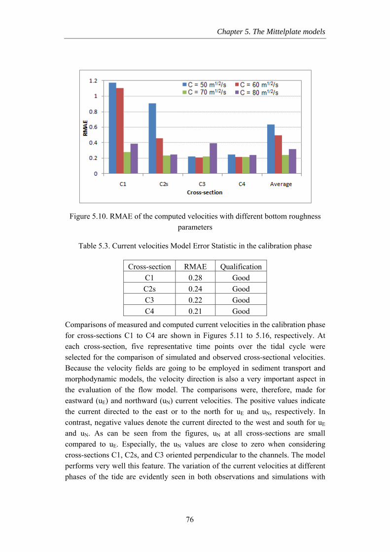
Chapter 5. The Mittelplate models
Figure 5.10. RMAE of the co
Table 5.3. Current velociti
Cross-sectiC1 C2s C3 C4
Comparisons of measured and for cross-sections C1 to C4 aeach cross-section, five represelected for the comparison ofBecause the velocity fields armorphodynamic models, the vthe evaluation of the flow meastward (uE) and northward (the current directed to the eacontrast, negative values denoand uN. As can be seen fromcompared to uE. Especially, tcross-sections C1, C2s, and C3performs very well this featurephases of the tide are evident
s
mputed velocities with different bottom roughness parameters
es Model Error Statistic in the calibration phase
on RMAE Qualification 0.28 Good 0.24 Good 0.22 Good 0.21 Good
computed current velocities in the calibration phase re shown in Figures 5.11 to 5.16, respectively. At sentative time points over the tidal cycle were simulated and observed cross-sectional velocities. e going to be employed in sediment transport and elocity direction is also a very important aspect in odel. The comparisons were, therefore, made for uN) current velocities. The positive values indicate st or to the north for uE and uN, respectively. In te the current directed to the west and south for uE
the figures, uN at all cross-sections are small he uN values are close to zero when considering oriented perpendicular to the channels. The model . The variation of the current velocities at different ly seen in both observations and simulations with
76
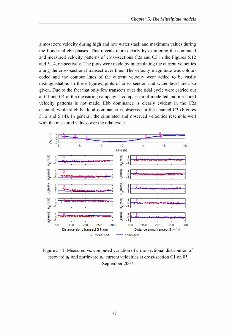
Chapter 5. The Mittelplate models
almost zero velocity during high and low water slack and maximum values during the flood and ebb phases. This reveals more clearly by examining the computed and measured velocity patterns of cross-sections C2s and C3 in the Figures 5.12 and 5.14, respectively. The plots were made by interpolating the current velocities along the cross-sectional transect over time. The velocity magnitude was colour-coded and the contour lines of the current velocity were added to be easily distinguishable. In these figures, plots of cross-section and water level are also given. Due to the fact that only few transects over the tidal cycle were carried out at C1 and C4 in the measuring campaigns, comparison of modelled and measured velocity patterns is not made. Ebb dominance is clearly evident in the C2s channel, while slightly flood dominance is observed in the channel C3 (Figures 5.12 and 5.14). In general, the simulated and observed velocities resemble well with the measured values over the tidal cycle.
Figure 5.11. Measured vs. computed variation of cross-sectional distribution of eastward uE and northward uN current velocities at cross-section C1 on 05
September 2007
77
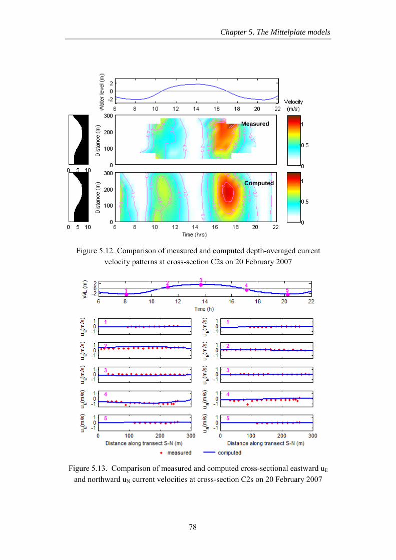
Chapter 5. The Mittelplate models
Figure 5.12. Comparison of measured and comvelocity patterns at cross-section C2s o
Figure 5.13. Comparison of measured and compuand northward uN current velocities at cross-sec
78
Measured
pun
tetio
Computed
ted depth-averaged current 20 February 2007
d cross-sectional eastward uE n C2s on 20 February 2007
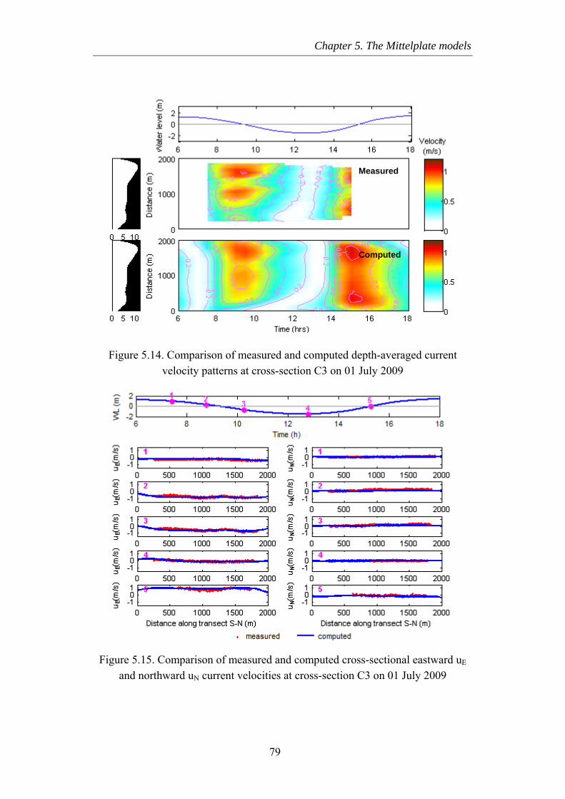
Chapter 5. The Mittelplate models
Measured
Computed
Figure 5.14. Comparison of measured and computed depth-averaged current velocity patterns at cross-section C3 on 01 July 2009
Figure 5.15. Comparison of measured and computed cross-sectional eastward uE and northward uN current velocities at cross-section C3 on 01 July 2009
79
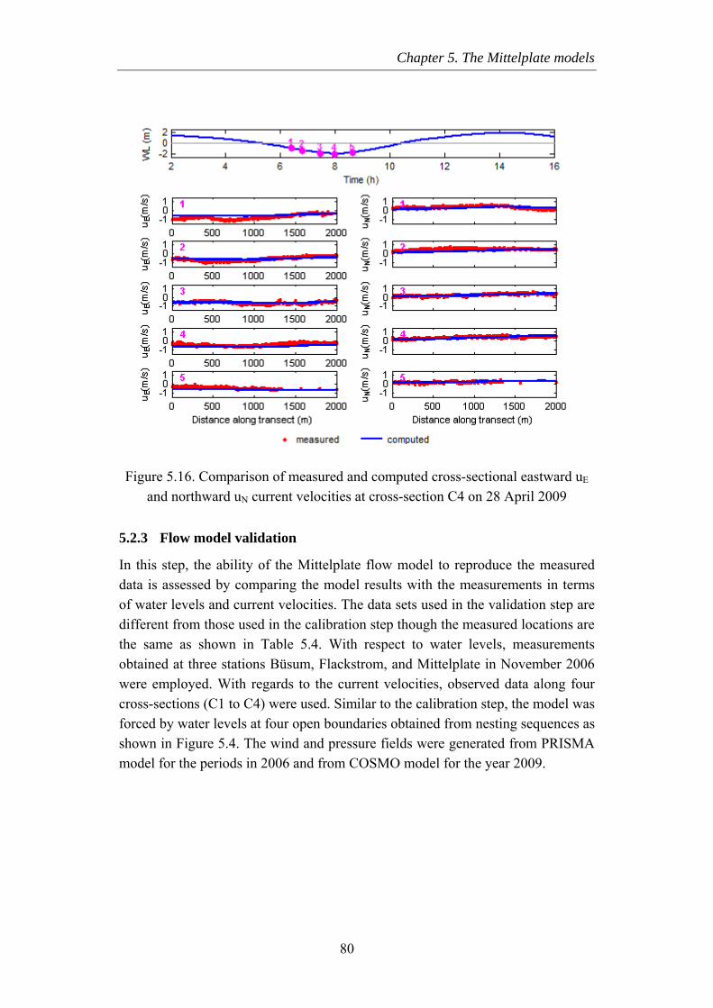
Chapter 5. The Mittelplate models
Figure 5.16. Comparison of measured and computed cross-sectional eastward uE and northward uN current velocities at cross-section C4 on 28 April 2009
5.2.3 Flow model validation
In this step, the ability of the Mittelplate flow model to reproduce the measured data is assessed by comparing the model results with the measurements in terms of water levels and current velocities. The data sets used in the validation step are different from those used in the calibration step though the measured locations are the same as shown in Table 5.4. With respect to water levels, measurements obtained at three stations Büsum, Flackstrom, and Mittelplate in November 2006 were employed. With regards to the current velocities, observed data along four cross-sections (C1 to C4) were used. Similar to the calibration step, the model was forced by water levels at four open boundaries obtained from nesting sequences as shown in Figure 5.4. The wind and pressure fields were generated from PRISMA model for the periods in 2006 and from COSMO model for the year 2009.
80
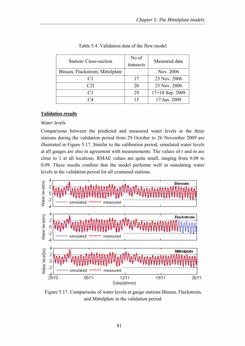
Chapter 5. The Mittelplate models
Table 5.4. Validation data of the flow model
Station/ Cross-section No of
transects Measured date
Büsum, Flackstrom, Mittelplate Nov. 2006 C1 17 23 Nov. 2006 C2l 20 23 Nov. 2006 C3 29 17+18 Sep. 2009 C4 15 17 Jun. 2009
Validation results
Water levels
Comparisons between the predicted and measured water levels at the three stations during the validation period from 29 October to 26 November 2009 are illustrated in Figure 5.17. Similar to the calibration period, simulated water levels at all gauges are also in agreement with measurements. The values of r and m are close to 1 at all locations. RMAE values are quite small, ranging from 0.08 to 0.09. These results confirm that the model performs well in simulating water levels in the validation period for all examined stations.
Figure 5.17. Comparisons of water levels at gauge stations Büsum, Flackstrom, and Mittelplate in the validation period
81
Chapter 5. The Mittelplate models
Current velocities
Comparisons of measured and computed current velocities in the validation phase for cross-sections C1 to C4 are shown in Figures 5.18 to 5.25. In the Figures 5.18, 5.20, 5.22, and 5.24 the measured and computed variation of current velocities along cross-section over time is presented. The model slightly overestimates the depth-averaged current velocities at cross-sections C1, C2l, and C3. Generally, both measurements and model results at all cross-sections show the variation of current velocities during different phases of the tidal cycle well. Close examination the Figure 5.20 for cross-section C2l, it shows that the flow is stronger in the connected channel than in the Trischenflinge channel during flood phase, while opposite trend is found in the ebb phase. Considering the Trischenflinge tidal channel at the cross-sections C1 and C2l, the flow is more predominant during ebb phase than flood phase with the measured peak ebb value of about 1 m/s (Figures 5.18 and 5.20). In contrast, the current velocities at cross-section C3 and at the connected channel south of Trischenflinge (C2l) are slightly stronger during flood than ebb phase (Figures 5.20 and 5.22). These show up both in the measurements and model results for cross-sections C2l and C3. Although no measured data are available during the ebb phase at C1 for the assessment, the model reveals this trend. Current flowing through cross-section C3 is found to be stronger than C4 (Figures 5.22 and 5.24).
Comparisons of the observed and simulated northward and eastward current velocities at five selected time points in the tidal cycle are presented as shown in the Figures 5.19, 5.21, 5.23, and 5.25 for cross-sections C1 to C4, respectively. The computed current velocities fit very well with the measurements. The northward current velocity is quite small in comparison with the eastward velocity, which was also observed in the calibration period.
Table 5.5 lists the statistical parameter RMAE obtained from comparisons of measured and computed current velocities at four cross-sections during validation period. The resulting RMAE values show better agreement at cross-section C3 and C4 located further to the sea than at cross-sections C1 and C2l, which is also found in the calibration step. The RMAE varies between 0.19 and 0.4, showing good to fair model performance, according to the qualification given in Table 2.1.
82
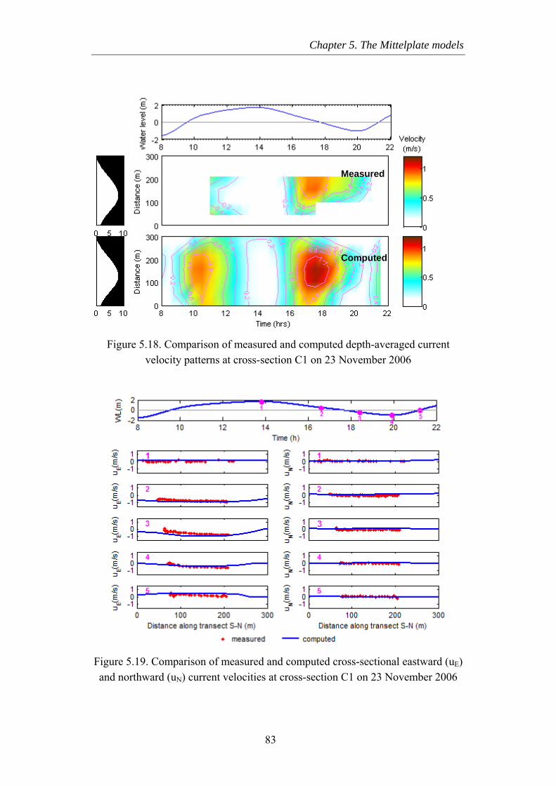
Chapter 5. The Mittelplate models
Figure 5.18. Comparison of measured and compuvelocity patterns at cross-section C1 on
Figure 5.19. Comparison of measured and computeand northward (uN) current velocities at cross-secti
83
Measured
Computedted depth-averaged current 23 November 2006
d cross-sectional eastward (uE) on C1 on 23 November 2006
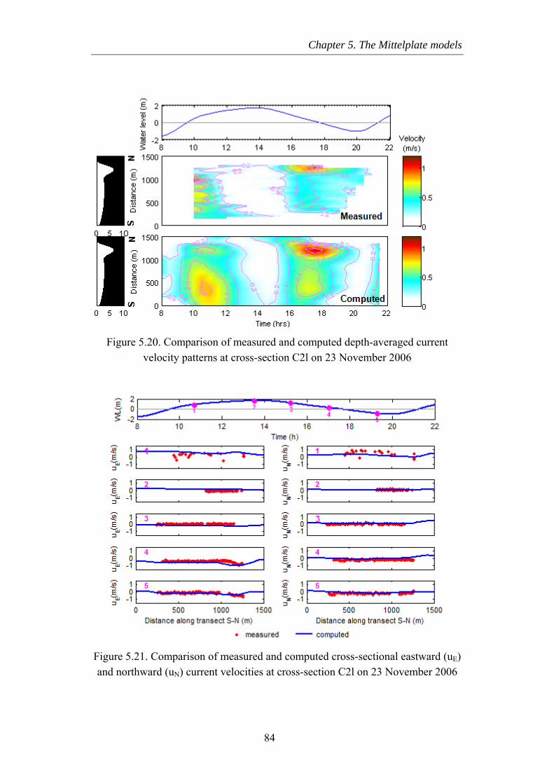
Chapter 5. The Mittelplate models
Figure 5.20. Comparison of measured and computed depth-averaged current velocity patterns at cross-section C2l on 23 November 2006
Figure 5.21. Comparison of measured and computed cross-sectional eastward (uE) and northward (uN) current velocities at cross-section C2l on 23 November 2006
84
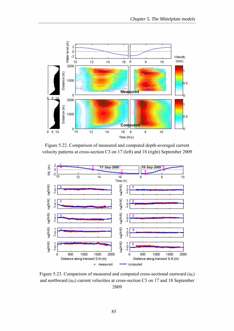
Chapter 5. The Mittelplate models
d
Figure 5.22. Comparison of measurevelocity patterns at cross-section C3 o
Figure 5.23. Comparison of measured aand northward (uN) current velocities at
2
8
Measure
Computedd and computed depth-averaged current n 17 (left) and 18 (right) September 2009
nd computed cross-sectional eastward (uE) cross-section C3 on 17 and 18 September 009
5
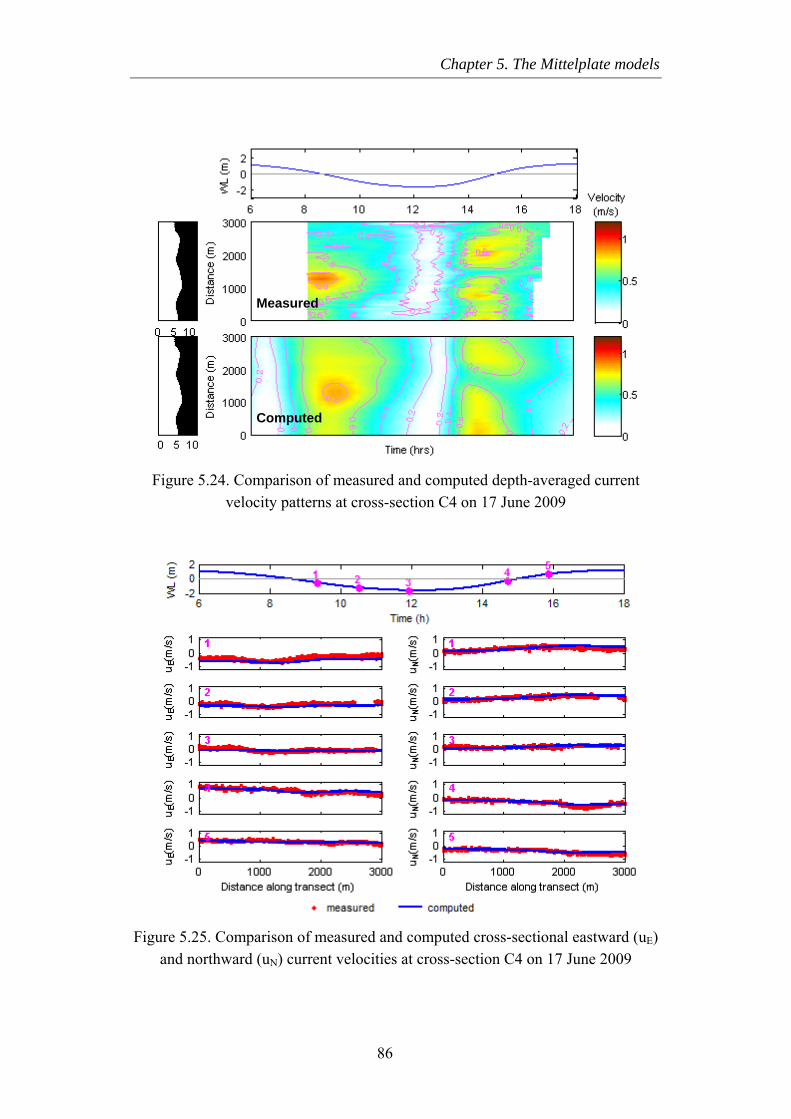
Chapter 5. The Mittelplate models
d
Figure 5.24.v
Figure 5.25. Coand northw
Measure
ComputedComparison of measured and computed depth-averaged current elocity patterns at cross-section C4 on 17 June 2009
mparison of measured and computed cross-sectional eastward (uE) ard (uN) current velocities at cross-section C4 on 17 June 2009
86
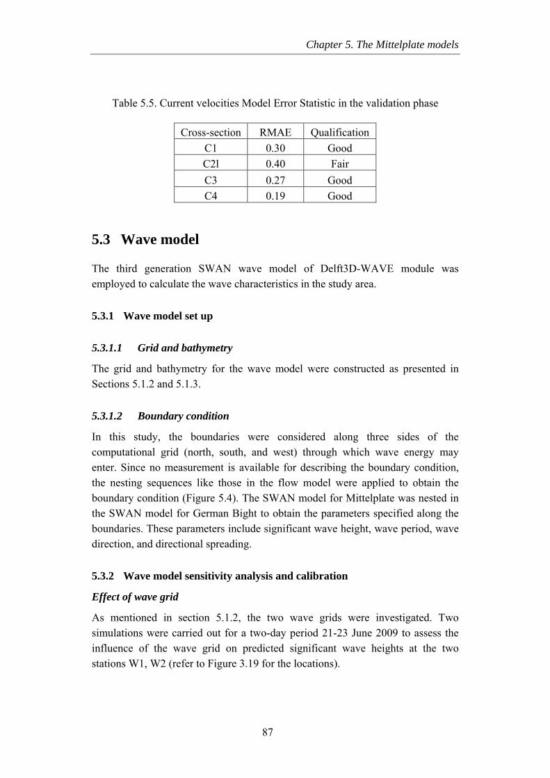
Chapter 5. The Mittelplate models
Table 5.5. Current velocities Model Error Statistic in the validation phase
Cross-section RMAE Qualification C1 0.30 Good C2l 0.40 Fair C3 0.27 Good C4 0.19 Good
5.3 Wave model
The third generation SWAN wave model of Delft3D-WAVE module was employed to calculate the wave characteristics in the study area.
5.3.1 Wave model set up
5.3.1.1 Grid and bathymetry
The grid and bathymetry for the wave model were constructed as presented in Sections 5.1.2 and 5.1.3.
5.3.1.2 Boundary condition
In this study, the boundaries were considered along three sides of the computational grid (north, south, and west) through which wave energy may enter. Since no measurement is available for describing the boundary condition, the nesting sequences like those in the flow model were applied to obtain the boundary condition (Figure 5.4). The SWAN model for Mittelplate was nested in the SWAN model for German Bight to obtain the parameters specified along the boundaries. These parameters include significant wave height, wave period, wave direction, and directional spreading.
5.3.2 Wave model sensitivity analysis and calibration
Effect of wave grid
As mentioned in section 5.1.2, the two wave grids were investigated. Two simulations were carried out for a two-day period 21-23 June 2009 to assess the influence of the wave grid on predicted significant wave heights at the two stations W1, W2 (refer to Figure 3.19 for the locations).
87
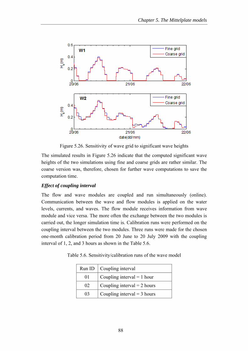
Chapter 5. The Mittelplate models
Figure 5.26. Sensitivity of wave grid to significant wave heights
The simulated results in Figure 5.26 indicate that the computed significant wave heights of the two simulations using fine and coarse grids are rather similar. The coarse version was, therefore, chosen for further wave computations to save the computation time.
Effect of coupling interval
The flow and wave modules are coupled and run simultaneously (online). Communication between the wave and flow modules is applied on the water levels, currents, and waves. The flow module receives information from wave module and vice versa. The more often the exchange between the two modules is carried out, the longer simulation time is. Calibration runs were performed on the coupling interval between the two modules. Three runs were made for the chosen one-month calibration period from 20 June to 20 July 2009 with the coupling interval of 1, 2, and 3 hours as shown in the Table 5.6.
Table 5.6. Sensitivity/calibration runs of the wave model
Run ID Coupling interval
01 Coupling interval = 1 hour
02 Coupling interval = 2 hours
03 Coupling interval = 3 hours
88
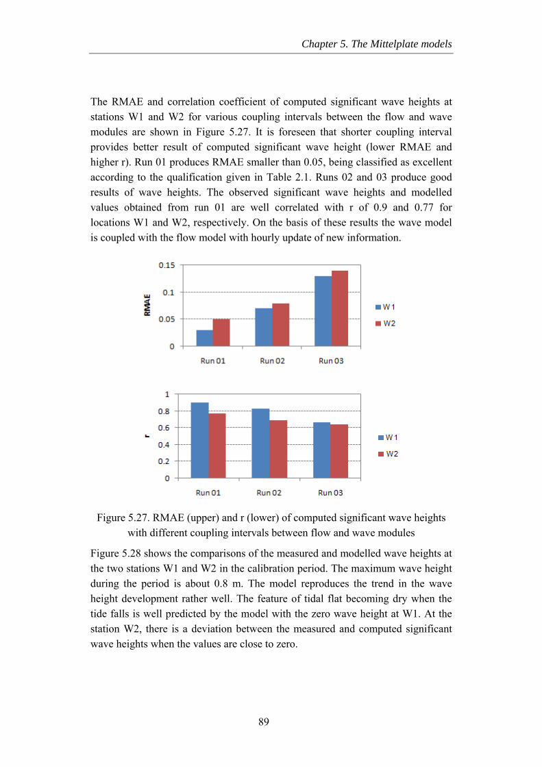
Chapter 5. The Mittelplate models
The RMAE and correlation coefficient of computed significant wave heights at stations W1 and W2 for various coupling intervals between the flow and wave modules are shown in Figure 5.27. It is foreseen that shorter coupling interval provides better result of computed significant wave height (lower RMAE and higher r). Run 01 produces RMAE smaller than 0.05, being classified as excellent according to the qualification given in Table 2.1. Runs 02 and 03 produce good results of wave heights. The observed significant wave heights and modelled values obtained from run 01 are well correlated with r of 0.9 and 0.77 for locations W1 and W2, respectively. On the basis of these results the wave model is coupled with the flow model with hourly update of new information.
Figure 5.27. RMAE (upper) and r (lower) of computed significant wave heights with different coupling intervals between flow and wave modules
Figure 5.28 shows the comparisons of the measured and modelled wave heights at the two stations W1 and W2 in the calibration period. The maximum wave height during the period is about 0.8 m. The model reproduces the trend in the wave height development rather well. The feature of tidal flat becoming dry when the tide falls is well predicted by the model with the zero wave height at W1. At the station W2, there is a deviation between the measured and computed significant wave heights when the values are close to zero.
89
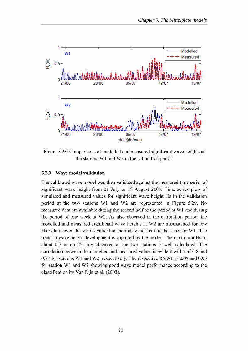
Chapter 5. The Mittelplate models
Figure 5.28. Comparisons of modelled and measured significant wave heights at the stations W1 and W2 in the calibration period
5.3.3 Wave model validation
The calibrated wave model was then validated against the measured time series of significant wave height from 21 July to 19 August 2009. Time series plots of simulated and measured values for significant wave height Hs in the validation period at the two stations W1 and W2 are represented in Figure 5.29. No measured data are available during the second half of the period at W1 and during the period of one week at W2. As also observed in the calibration period, the modelled and measured significant wave heights at W2 are mismatched for low Hs values over the whole validation period, which is not the case for W1. The trend in wave height development is captured by the model. The maximum Hs of about 0.7 m on 25 July observed at the two stations is well calculated. The correlation between the modelled and measured values is evident with r of 0.8 and 0.77 for stations W1 and W2, respectively. The respective RMAE is 0.09 and 0.05 for station W1 and W2 showing good wave model performance according to the classification by Van Rijn et al. (2003).
90
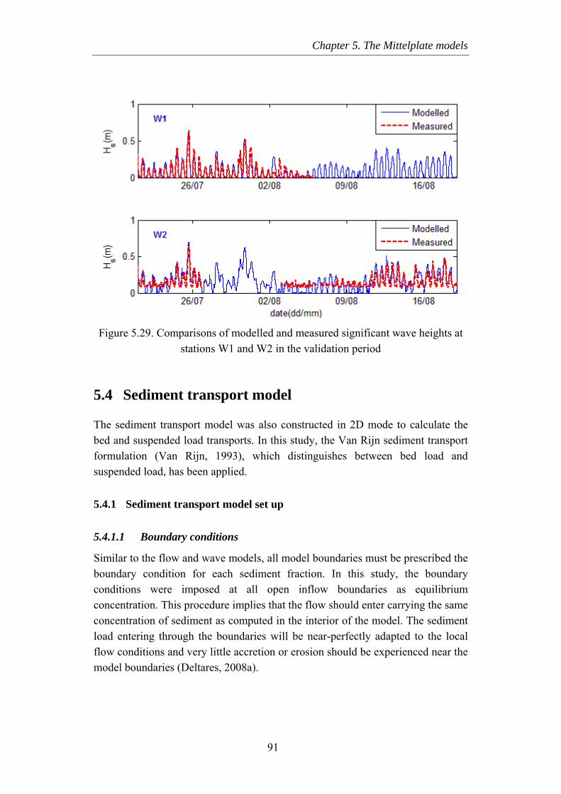
Chapter 5. The Mittelplate models
Figure 5.29. Comparisons of modelled and measured significant wave heights at stations W1 and W2 in the validation period
5.4 Sediment transport model
The sediment transport model was also constructed in 2D mode to calculate the bed and suspended load transports. In this study, the Van Rijn sediment transport formulation (Van Rijn, 1993), which distinguishes between bed load and suspended load, has been applied.
5.4.1 Sediment transport model set up
5.4.1.1 Boundary conditions
Similar to the flow and wave models, all model boundaries must be prescribed the boundary condition for each sediment fraction. In this study, the boundary conditions were imposed at all open inflow boundaries as equilibrium concentration. This procedure implies that the flow should enter carrying the same concentration of sediment as computed in the interior of the model. The sediment load entering through the boundaries will be near-perfectly adapted to the local flow conditions and very little accretion or erosion should be experienced near the model boundaries (Deltares, 2008a).
91
Chapter 5. The Mittelplate models
5.4.1.2 Non-erodible layer
As discussed in Section 3.6.1, the subsoil of the Dithmarchen Bight including Mittelplate area consists of alternating erodible layers and non-erodible layers of clay (Dithmarscher Klei). The deposit clay layer was also detected at the Trischenfinge channel as the results from the detailed analysis of the bathymetric measurement in Chapter 4. These hard layers were included in the model by adjusting sediment availability above them which is available for sediment transport.
5.4.1.3 Sediment composition
In this study, two sediment fractions were considered: cohesive and non-cohesive sediment. The non-cohesive sediment sizes were set to be uniform over the whole domain. Two grain sizes, d50 = 140 µm and 200 µm, were chosen as one of the calibration parameters in the following section. As described in Section 3.6.3, the mud content in the less exposed tidal channels is generally greater than 5%, attaining maximum values of 80% and about 50% samples having more than 10% of mud. In this study, the mud content of 20% was distributed in the channels.
5.4.2 Sediment transport model sensitivity and calibration
The sediment transport model was calibrated using the data obtained from three measured campaigns in the year 2009 along four cross-sections C3, C4, C5, and C6 as shown in Figure 5.30 and Table 5.7. On 01 July, concentration data at seven stations were recorded along cross-section C3. On 17 June, eight stations (red in Figure 5.30) along C4 were monitored, whereas three stations were available on 28 October at C5 and C6. All data sets contain suspended sediment concentration throughout a tidal cycle at stations along cross-sections.
92
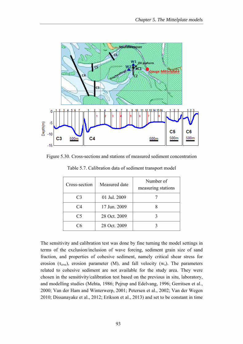
Chapter 5. The Mittelplate models
Figure 5.30. Cross-sections and stations of measured sediment concentration
Table 5.7. Calibration data of sediment transport model
Cross-section Measured date Number of
measuring stations
C3 01 Jul. 2009 7
C4 17 Jun. 2009 8
C5 28 Oct. 2009 3
C6 28 Oct. 2009 3
The sensitivity and calibration test was done by fine turning the model settings in terms of the exclusion/inclusion of wave forcing, sediment grain size of sand fraction, and properties of cohesive sediment, namely critical shear stress for erosion (τcr,e), erosion parameter (M), and fall velocity (ws). The parameters related to cohesive sediment are not available for the study area. They were chosen in the sensitivity/calibration test based on the previous in situ, laboratory, and modelling studies (Mehta, 1986; Pejrup and Edelvang, 1996; Gerritsen et al., 2000; Van der Ham and Winterwerp, 2001; Petersen et al., 2002; Van der Wegen 2010; Dissanayake et al., 2012; Erikson et al., 2013) and set to be constant in time
93
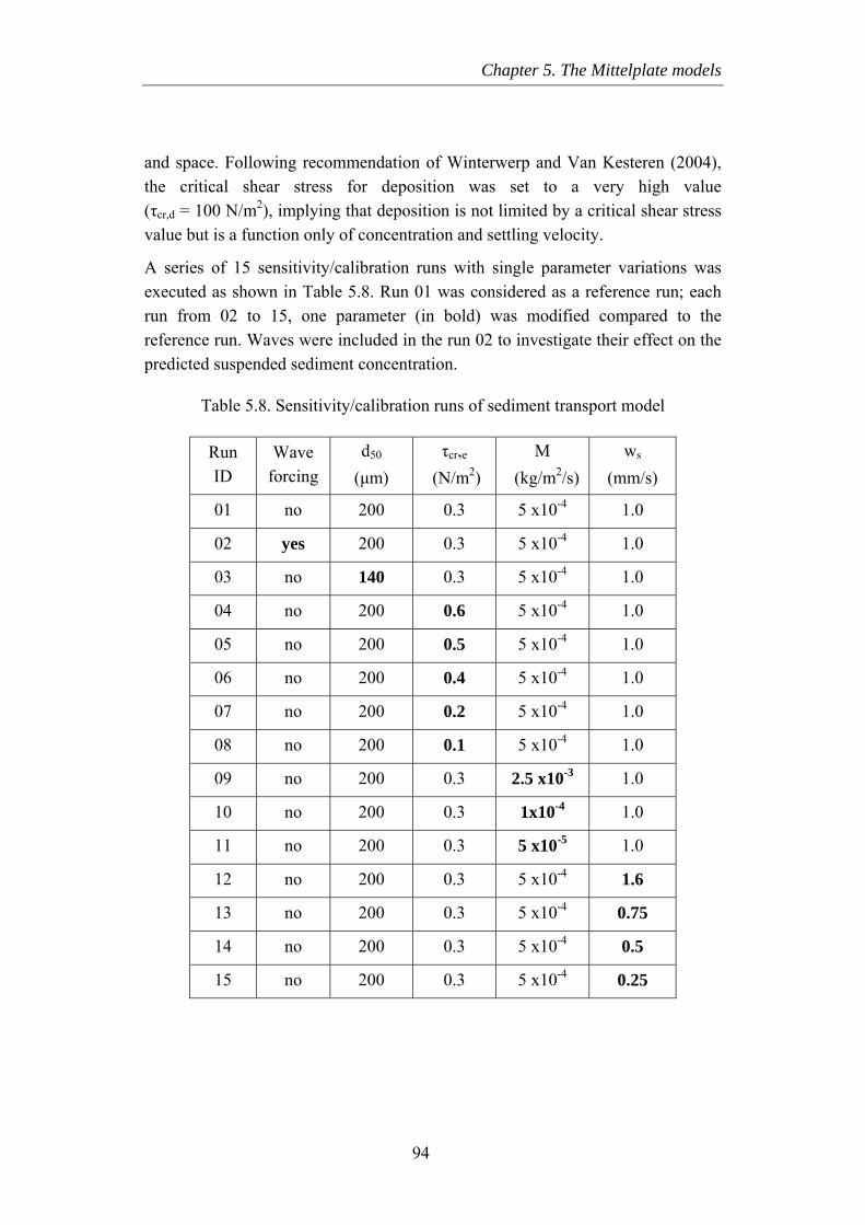
Chapter 5. The Mittelplate models
and space. Following recommendation of Winterwerp and Van Kesteren (2004), the critical shear stress for deposition was set to a very high value (τcr,d = 100 N/m2), implying that deposition is not limited by a critical shear stress value but is a function only of concentration and settling velocity.
A series of 15 sensitivity/calibration runs with single parameter variations was executed as shown in Table 5.8. Run 01 was considered as a reference run; each run from 02 to 15, one parameter (in bold) was modified compared to the reference run. Waves were included in the run 02 to investigate their effect on the predicted suspended sediment concentration.
Table 5.8. Sensitivity/calibration runs of sediment transport model
Run ID
Wave forcing
d50
(µm) τcr,e
(N/m2) M
(kg/m2/s) ws
(mm/s)
01 no 200 0.3 5 x10⁻⁴ 1.0
02 yes 200 0.3 5 x10⁻⁴ 1.0
03 no 140 0.3 5 x10⁻⁴ 1.0
04 no 200 0.6 5 x10⁻⁴ 1.0
05 no 200 0.5 5 x10⁻⁴ 1.0
06 no 200 0.4 5 x10⁻⁴ 1.0
07 no 200 0.2 5 x10⁻⁴ 1.0
08 no 200 0.1 5 x10⁻⁴ 1.0
09 no 200 0.3 2.5 x10⁻³ 1.0
10 no 200 0.3 1x10⁻⁴ 1.0
11 no 200 0.3 5 x10⁻⁵ 1.0
12 no 200 0.3 5 x10⁻⁴ 1.6
13 no 200 0.3 5 x10⁻⁴ 0.75
14 no 200 0.3 5 x10⁻⁴ 0.5
15 no 200 0.3 5 x10⁻⁴ 0.25
94
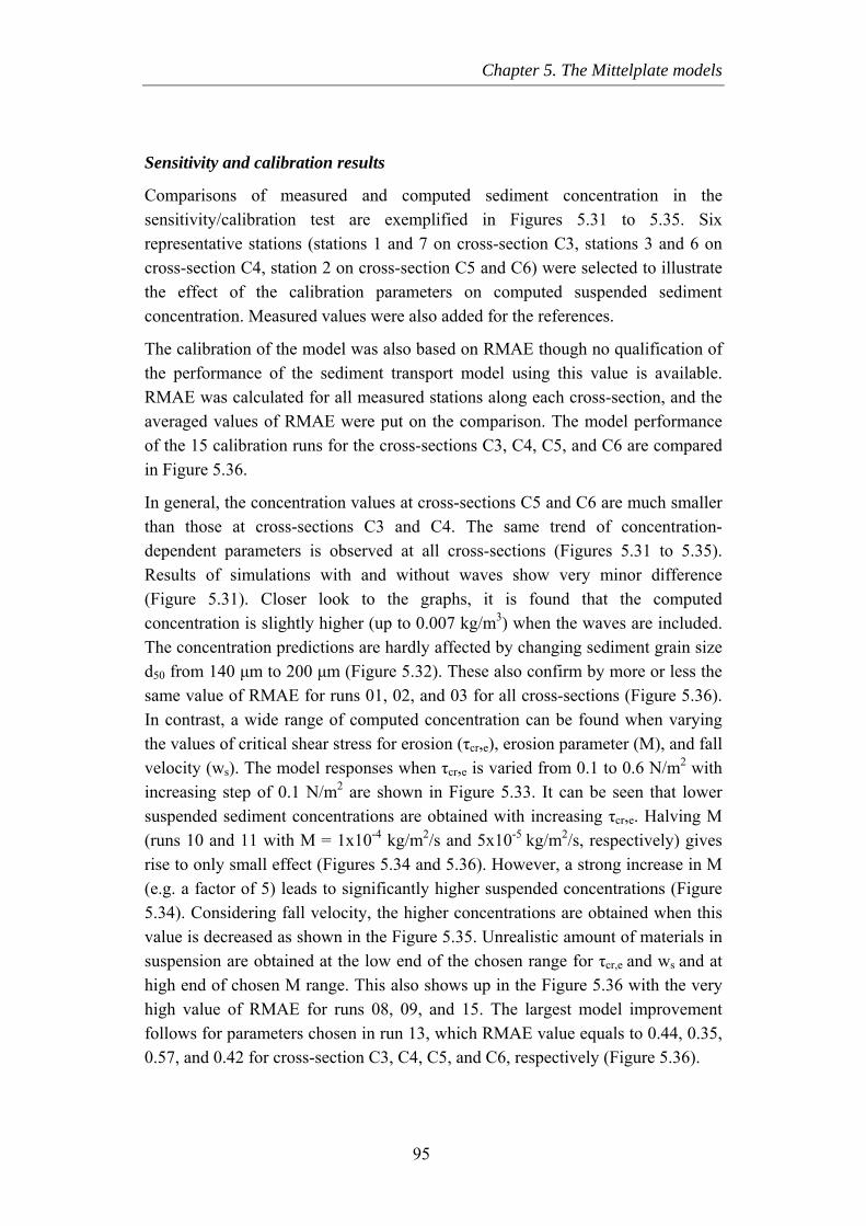
Chapter 5. The Mittelplate models
Sensitivity and calibration results
Comparisons of measured and computed sediment concentration in the sensitivity/calibration test are exemplified in Figures 5.31 to 5.35. Six representative stations (stations 1 and 7 on cross-section C3, stations 3 and 6 on cross-section C4, station 2 on cross-section C5 and C6) were selected to illustrate the effect of the calibration parameters on computed suspended sediment concentration. Measured values were also added for the references.
The calibration of the model was also based on RMAE though no qualification of the performance of the sediment transport model using this value is available. RMAE was calculated for all measured stations along each cross-section, and the averaged values of RMAE were put on the comparison. The model performance of the 15 calibration runs for the cross-sections C3, C4, C5, and C6 are compared in Figure 5.36.
In general, the concentration values at cross-sections C5 and C6 are much smaller than those at cross-sections C3 and C4. The same trend of concentration-dependent parameters is observed at all cross-sections (Figures 5.31 to 5.35). Results of simulations with and without waves show very minor difference (Figure 5.31). Closer look to the graphs, it is found that the computed concentration is slightly higher (up to 0.007 kg/m3) when the waves are included. The concentration predictions are hardly affected by changing sediment grain size d50 from 140 µm to 200 µm (Figure 5.32). These also confirm by more or less the same value of RMAE for runs 01, 02, and 03 for all cross-sections (Figure 5.36). In contrast, a wide range of computed concentration can be found when varying the values of critical shear stress for erosion (τcr,e), erosion parameter (M), and fall velocity (ws). The model responses when τcr,e is varied from 0.1 to 0.6 N/m2 with increasing step of 0.1 N/m2 are shown in Figure 5.33. It can be seen that lower suspended sediment concentrations are obtained with increasing τcr,e. Halving M (runs 10 and 11 with M = 1x10⁻⁴ kg/m2/s and 5x10⁻⁵ kg/m2/s, respectively) gives rise to only small effect (Figures 5.34 and 5.36). However, a strong increase in M (e.g. a factor of 5) leads to significantly higher suspended concentrations (Figure 5.34). Considering fall velocity, the higher concentrations are obtained when this value is decreased as shown in the Figure 5.35. Unrealistic amount of materials in suspension are obtained at the low end of the chosen range for τcr,e and ws and at high end of chosen M range. This also shows up in the Figure 5.36 with the very high value of RMAE for runs 08, 09, and 15. The largest model improvement follows for parameters chosen in run 13, which RMAE value equals to 0.44, 0.35, 0.57, and 0.42 for cross-section C3, C4, C5, and C6, respectively (Figure 5.36).
95
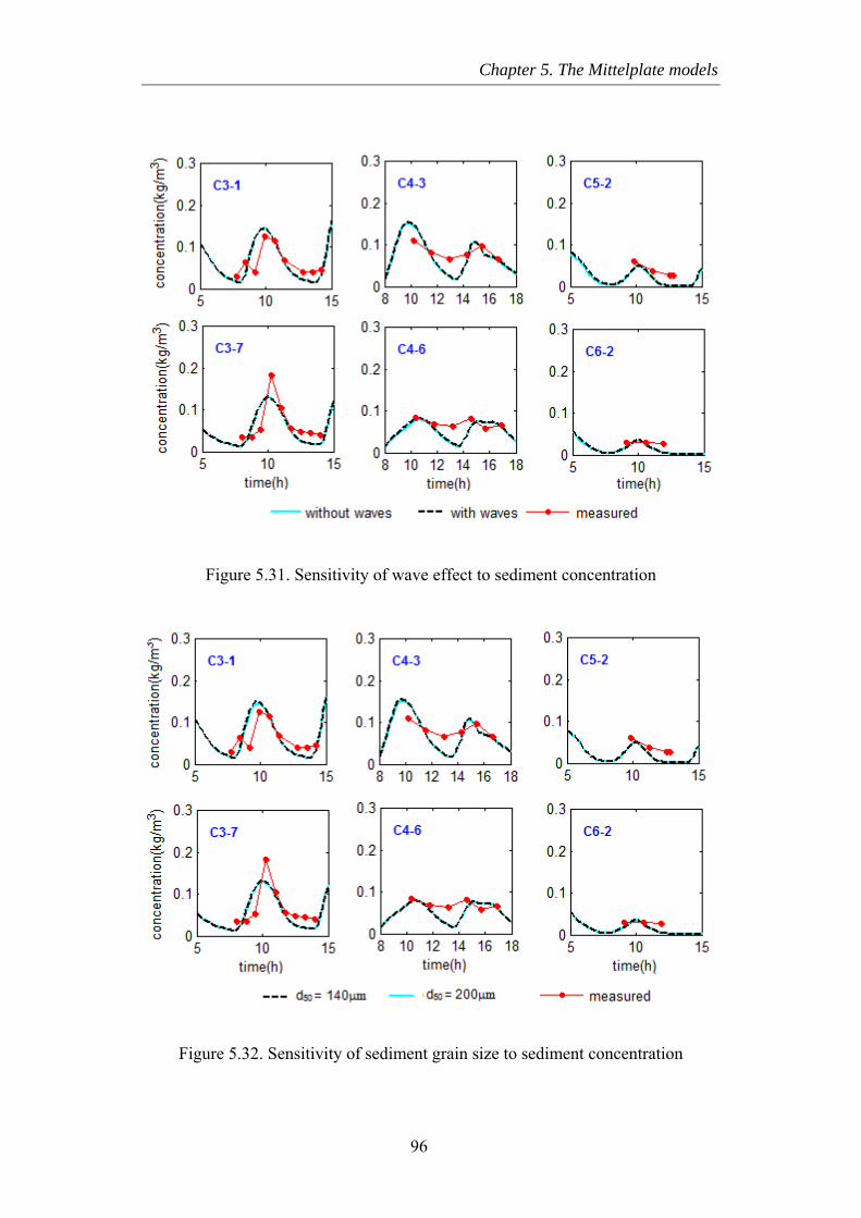
Chapter 5. The Mittelplate models
Figure 5.31. Sensitivity of wave effect to sediment concentration
Figure 5.32. Sensitivity of sediment grain size to sediment concentration
96
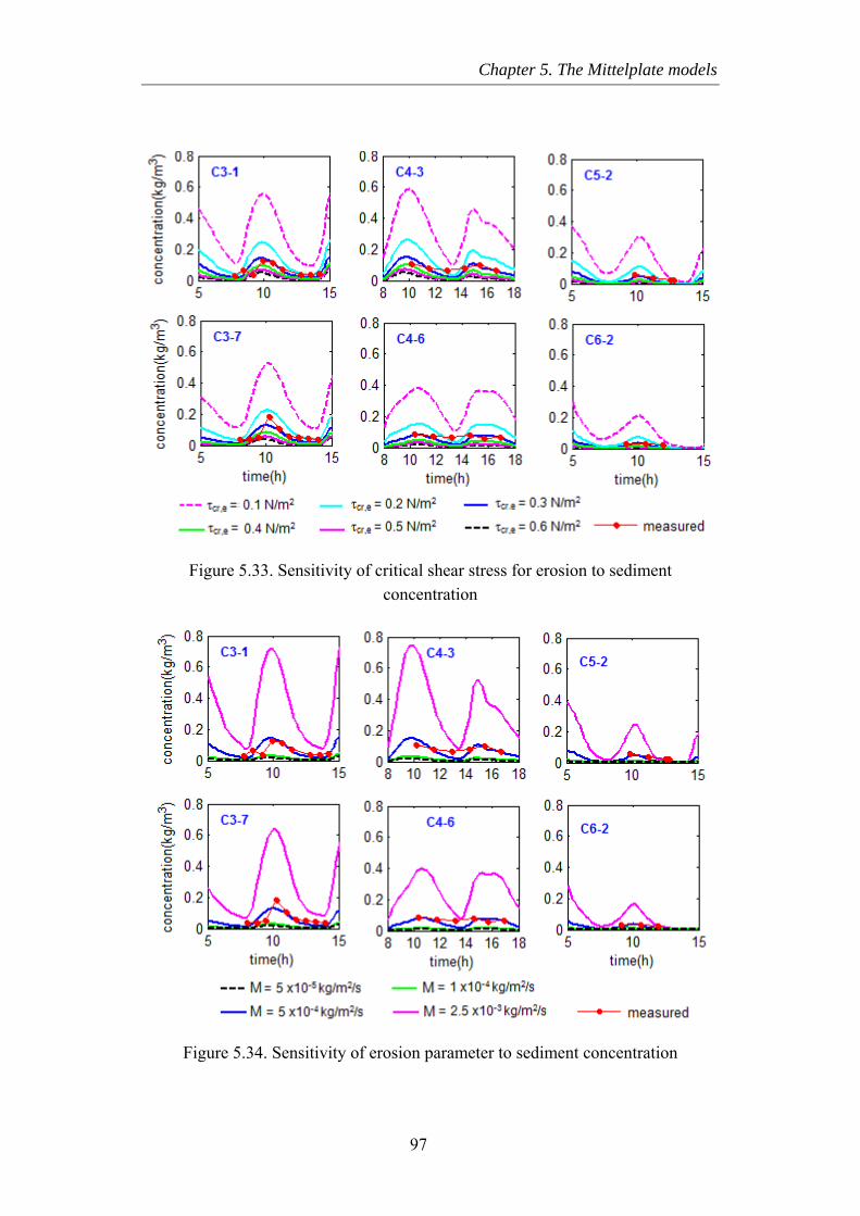
Chapter 5. The Mittelplate models
Figure 5.33. Sensitivity of critical shear stress for erosion to sediment concentration
Figure 5.34. Sensitivity of erosion parameter to sediment concentration
97
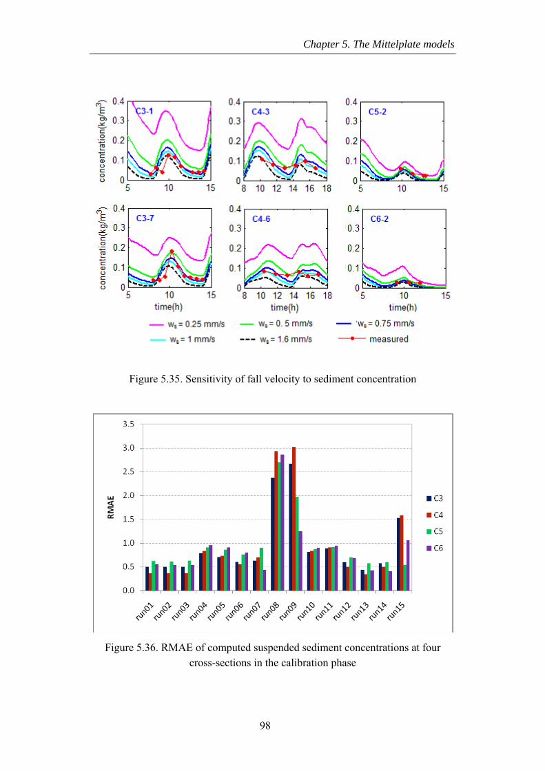
Chapter 5. The Mittelplate models
Figure 5.35. Sensitivity of fall velocity to sediment concentration
Figure 5.36. RMAE of computed suspended sediment concentrations at four cross-sections in the calibration phase
98
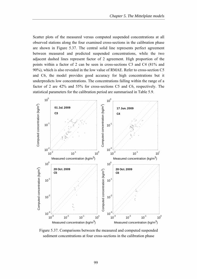
Chapter 5. The Mittelplate models
Scatter plots of the measured versus computed suspended concentrations at all observed stations along the four examined cross-sections in the calibration phase are shown in Figure 5.37. The central solid line represents perfect agreement between measured and predicted suspended concentrations, while the two adjacent dashed lines represent factor of 2 agreement. High proportion of the points within a factor of 2 can be seen in cross-sections C3 and C4 (81% and 90%), which is also revealed in the low value of RMAE. Refer to cross-section C5 and C6, the model provides good accuracy for high concentrations but it underpredicts low concentrations. The concentrations falling within the range of a factor of 2 are 42% and 55% for cross-sections C5 and C6, respectively. The statistical parameters for the calibration period are summarised in Table 5.9.
10-2 10-1 10010-2
10-1
100
Measured concentration (kg/m3)
C10-2 10-1 100
10-2
10-1
100
Measured concentration (kg/m3)
Computed concentration (kg/m
3)
Com
pute
d co
ncen
tratio
n (k
g/m
3 )
omputed concentration (kg/m
3)C
ompu
ted
conc
entra
tion
(kg/
m3 )
01 Jul. 2009
C317 Jun. 2009
C4
10-3 10-2 10-1 10010-3
10-2
10-1
100
Measured concentration (kg/m3)
C10-3 10-2 10-1 100
10-3
10-2
10-1
100
Measured concentration (kg/m3)
Computed concentration (kg/m
3)
Com
pute
d co
ncen
tratio
n (k
g/m
3 )
omputed concentration (kg/m)28 Oct. 2009
C5 3 28 Oct. 2009C6
Com
pute
d co
ncen
tratio
n (k
g/m
3 )
Figure 5.37. Comparisons between the measured and computed suspended sediment concentrations at four cross-sections in the calibration phase
99
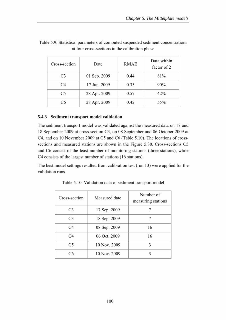
Chapter 5. The Mittelplate models
Table 5.9. Statistical parameters of computed suspended sediment concentrations at four cross-sections in the calibration phase
Cross-section Date RMAE Data within factor of 2
C3 01 Sep. 2009 0.44 81%
C4 17 Jun. 2009 0.35 90%
C5 28 Apr. 2009 0.57 42%
C6 28 Apr. 2009 0.42 55%
5.4.3 Sediment transport model validation
The sediment transport model was validated against the measured data on 17 and 18 September 2009 at cross-section C3, on 08 September and 06 October 2009 at C4, and on 10 November 2009 at C5 and C6 (Table 5.10). The locations of cross-sections and measured stations are shown in the Figure 5.30. Cross-sections C5 and C6 consist of the least number of monitoring stations (three stations), while C4 consists of the largest number of stations (16 stations).
The best model settings resulted from calibration test (run 13) were applied for the validation runs.
Table 5.10. Validation data of sediment transport model
Cross-section Measured date Number of
measuring stations
C3 17 Sep. 2009 7
C3 18 Sep. 2009 7
C4 08 Sep. 2009 16
C4 06 Oct. 2009 16
C5 10 Nov. 2009 3
C6 10 Nov. 2009 3
100
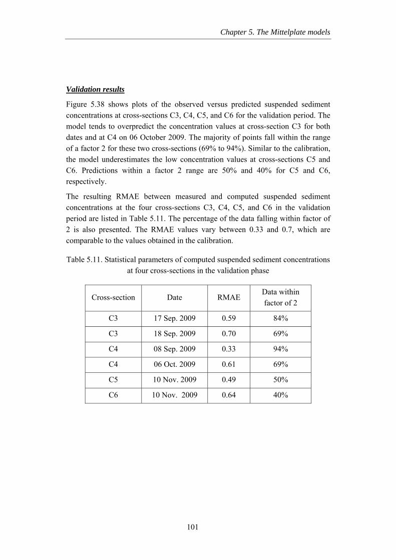
Chapter 5. The Mittelplate models
Validation results
Figure 5.38 shows plots of the observed versus predicted suspended sediment concentrations at cross-sections C3, C4, C5, and C6 for the validation period. The model tends to overpredict the concentration values at cross-section C3 for both dates and at C4 on 06 October 2009. The majority of points fall within the range of a factor 2 for these two cross-sections (69% to 94%). Similar to the calibration, the model underestimates the low concentration values at cross-sections C5 and C6. Predictions within a factor 2 range are 50% and 40% for C5 and C6, respectively.
The resulting RMAE between measured and computed suspended sediment concentrations at the four cross-sections C3, C4, C5, and C6 in the validation period are listed in Table 5.11. The percentage of the data falling within factor of 2 is also presented. The RMAE values vary between 0.33 and 0.7, which are comparable to the values obtained in the calibration.
Table 5.11. Statistical parameters of computed suspended sediment concentrations at four cross-sections in the validation phase
Cross-section Date RMAE Data within factor of 2
C3 17 Sep. 2009 0.59 84%
C3 18 Sep. 2009 0.70 69%
C4 08 Sep. 2009 0.33 94%
C4 06 Oct. 2009 0.61 69%
C5 10 Nov. 2009 0.49 50%
C6 10 Nov. 2009 0.64 40%
101
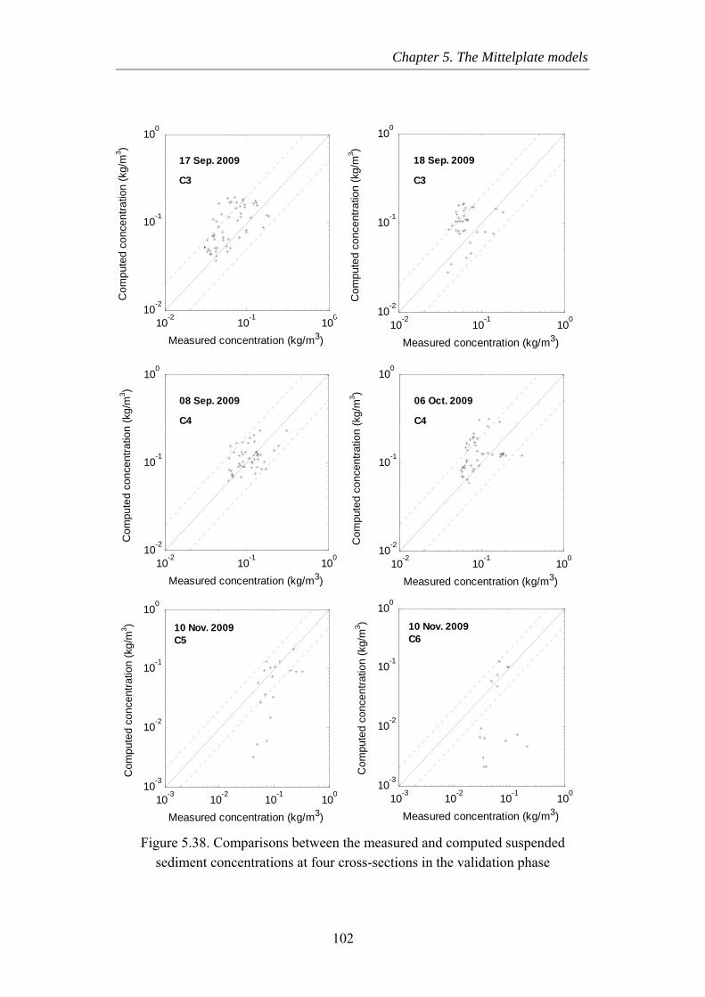
Chapter 5. The Mittelplate models
10-2 10-1 10010-2
10-1
100
Measured concentration (kg/m3)
Co
10-2 10-1 10010-2
10-1
100
Measured concentration (kg/m3)
Compuedconcenaonkm3)
t
trti (g/
17 Sep. 2009
C3
Com
pute
d co
ncen
tratio
n (k
g/m
3 )
mpuedconcenaonkm3
t
trti (g/
)18 Sep. 2009
C3
Com
pute
d co
ncen
tratio
n (k
g/m
3 )
10-2 10-1 10010-2
10-1
100
Measured concentration (kg/m3)
10-2 10-1 10010-2
10-1
100
Measured concentration (kg/m3)
Compuedconcenaonkm
t
trti (g/
3) 08 Sep. 2009
C4
Com
pute
d co
ncen
tratio
n (k
g/m
3 )
Cmpuedonenaon(m3
o
t cctrti kg/
)06 Oct. 2009
C4
Com
pute
d co
ncen
tratio
n (k
g/m
3 )
10-3 10-2 10-1 10010-3
10-2
10-1
100
Measured concentration (kg/m3)
Computed concentration (kg/m
3) 10 Nov. 2009C5
10-3 10-2 10-1 10010-3
10-2
10-1
100
Measured concentration (kg/m3)
Computed concentration (kg/m
3) 10 Nov. 2009C6
Com
pute
d co
ncen
tratio
n (k
g/m
3 )
Com
pute
d co
ncen
tratio
n (k
g/m
3 )
Figure 5.38. Comparisons between the measured and computed suspended sediment concentrations at four cross-sections in the validation phase
102
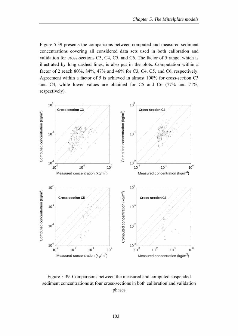
Chapter 5. The Mittelplate models
Figure 5.39 presents the comparisons between computed and measured sediment concentrations covering all considered data sets used in both calibration and validation for cross-sections C3, C4, C5, and C6. The factor of 5 range, which is illustrated by long dashed lines, is also put in the plots. Computation within a factor of 2 reach 80%, 84%, 47% and 46% for C3, C4, C5, and C6, respectively. Agreement within a factor of 5 is achieved in almost 100% for cross-section C3 and C4, while lower values are obtained for C5 and C6 (77% and 71%, respectively).
10-2 10-1 10010-2
10-1
100
Measured concentration (kg/m3)10-2 10-1 100
10-2
10-1
100
Measured concentration (kg/m3)
Computed concentration (kg/m
3)
Com
pute
d co
ncen
tratio
n (k
g/m
3 ) Cross section C3
Computed concentration (kg/m
3)
Com
pute
d co
ncen
tratio
n (k
g/m
3 ) Cross section C4
10-3 10-2 10-1 10010-3
10-2
10-1
100
Measured concentration (kg/m3)
C10-3 10-2 10-1 100
10-3
10-2
10-1
100
Measured concentration (kg/m3)
Computed concentration (kg/m
3)
Com
pute
d co
ncen
tratio
n (k
g/m
3 )
omputed concentration (kg/m
3)
Com
pute
d co
ncen
tratio
n (k
g/m
3 )
Cross section C5 Cross section C6
Figure 5.39. Comparisons between the measured and computed suspended sediment concentrations at four cross-sections in both calibration and validation
phases
103
Chapter 5. The Mittelplate models
5.5 Morphodynamic model
In the previous sections, the process models for simulating flow, wave, and sediment transport for the Mittelplate area have been set-up, calibrated, and validated. The calibration and the validation of those models showed their capability of reproducing the physical processes in the area. In this section, the morphodynamic model for the study area is developed in a medium-term scale based on the flow, wave, and sediment transport models described above.
As described in Chapter 2, the "morphological factor approach" in conjunction with the “representative period method” (Boon et al., 2002) was implemented in the medium-term morphodynamic model for the Mittelplate area. Applying the method proposed by Boon et al. (2002), one-month representative period covering two full spring-neap cycles was chosen for the determination of the boundary conditions for the individual process models. Benchmark simulations using the full time series of forcing were also implemented.
Figure 5.40 illustrates the flow chart of medium-term morphological modelling for the Mittelplate model. The boundary conditions (BC) for the flow and wave models are taken from nesting sequences as shown in the Figures 5.4 and 5.40. Wind, pressure and computed boundary conditions are then prescribed to the Mittelplate flow and wave models. The flow uses the updated wave field every one hour to calculate simultaneously the flow field, sediment transport and bed level change. The next wave computation uses the new flow field and morphology. The bathymetry is updated at each computational time step by multiplying erosion and deposition fluxes by a constant morphological scale factor (fMOR). The details of morphodynamic simulations and value of fMOR will be discussed in Chapter 6.
104
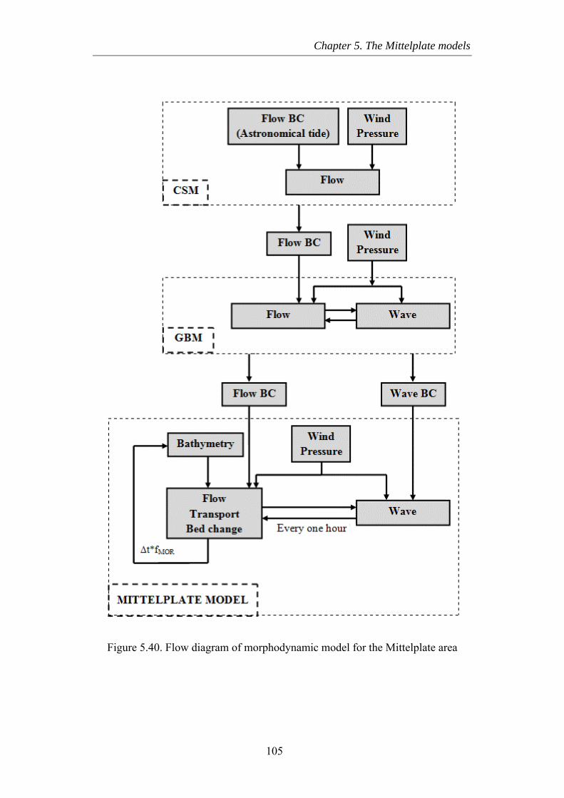
Chapter 5. The Mittelplate models
Figure 5.40. Flow diagram of morphodynamic model for the Mittelplate area
105
Chapter 5. The Mittelplate models
5.6 Discussion
In this chapter, the set-up, calibration, and validation of the Mittelplate Delft3D model for simulation of flow, wave, and sediment transport were presented. The resulting calibrated and validated models were adopted to set up the morphodynamic model in medium-term scale.
Various data sets were employed to evaluate the flow, wave, and sediment transport models. Model calibration and validation have been done qualitatively and quantitatively, involving both graphical analyses and statistics tests. A number of statistical parameters were used to assess the model performance. For the hydrodynamic results, the Relative Mean Absolute Error (RMAE), linear correlation coefficient (r), and the slope of best-fit line forced through the origin (m) were used. For the evaluation of sediment transport model, RMAE, factor of 2, and factor of 5 criteria were applied.
The results of computed water levels and current velocities showed that the model is capable of reproducing the hydrodynamics in the complex area. Although some deviation was observed at high and low water in some days during the calibration and validation periods, the calculated water levels were considered being well agreement with the measurements. The resulting RMAE was quite small, being around 0.1, and the r and m values are almost 1. The deviation can be introduced by the application of nesting procedure for the boundary condition of the model and the exclusion of waves in the flow simulations. The exclusion of wave effects, however, seems to be acceptable when considering the current velocities. This is due to the fact that the measured campaigns for the currents could only be done during calm weather conditions because of technical reasons such as requirements for the measuring devices and vessels. The resulting RMAE values of computed current velocity at four cross-sections varied from 0.19 to 0.4, being rated good and fair according to Van Rijn et al. (2003). Better model performance was obtained at cross-sections C3 and C4 located further to the sea than at C1 and C2. It is partly contributed by the location and shape of those considered channels. Cross-sections C3 and C4 are longer and deeper than the two others, making the velocity measurements by a moving vessel easier and more correct.
Current velocities along the five examined cross-sections showed the flood-ebb asymmetry. For the cross-sections C1, C2s, and C2l located at the Trischenflinge channel, ebb dominance of current velocity is obvious. In contrast, the current velocities at cross-section C3 and at the connected channel between shoals S1 and
106
Chapter 5. The Mittelplate models
S2 are flood dominated. The model represented the observed pattern quite well although deviations in the magnitude were found.
The achieved agreement between simulations and observations of current velocities is remarkable, considering the several factors. First, the application of depth-averaged model and nesting procedure contribute to the discrepancies between the model results and the nature. Other sources of errors are due to the fact that the measurements of current velocities were carried out from moving vessels, and the extrapolation procedure was applied to describe the velocity profiles over the entire water depth.
Regarding to the wave model, the model reproduced significant wave heights very well. The quantitative qualification based on the RMAE value revealed a very good agreement between the model results and observations. The measurements and computations showed small wave heights during the measuring campaigns. The reason is that the waves have broken along the outer margins of the area of interest. The discrepancies between the model and nature were found at station W2 when the waves being close to zero. Inspection of the wave measurements at this location, it was found that the measured wave heights reach the smallest values of about 0.1 m systematically. This deviation can be explained by the limitation of the used ADCP instrument in measuring low waves.
The sediment transport model was calibrated with the aim of obtaining appropriate parameter settings in terms of grain size of non-cohesive sediment and properties of cohesive sediment. The effect of waves on predicted suspended concentrations was also examined by coupling wave and flow models. It was found that the effect of waves on the sediment dynamics is negligible in the measuring campaigns which were carried out during the calm periods. Changing grain size between 140 µm and 200 µm did not have clear effect on the suspended concentration. In contrast, the model was very sensitive to the change of properties of mud fraction. Higher suspended sediment concentrations were induced with decreasing critical shear stress for erosion, decreasing fall velocity, and increasing erosion parameter. These are explained by the fact that when decreasing critical shear stress for erosion below which no erosion occurs, more sediments from the bed are eroded. A decrease in fall velocity means that settling is reduced and suspended concentrations are therefore higher. In contrast, an increase in erosion parameter enhances erosion, leading to more materials in suspension.
107
Chapter 5. The Mittelplate models
Although no qualification of RMAE value for the sediment transport has been published, it was used as a tool for the comparisons of the model performance when applying different model settings and for the comparisons of the model performance at different locations. The resulting RMAE values in the validation were in the range of 0.33 to 0.7, which are comparable with those obtained in calibration test. The percentage of the data within a factor of 2 deviation was generally high for cross-sections C3 and C4 in calibration and validation periods, accounting for 69% to 94% of the points. At cross-sections C5 and C6, the model underestimated the low concentration values and the data falling within a factor of 2 range reduced to a range of 40% - 55%. Considering all data sets at each cross-section, concentrations within a factor of 2 reached 80% and 84% for C3 and C4, respectively, whereas 47% and 46% were observed for C5 and C6. The percentage of data within a factor of 5 was almost 100% for cross-section C3 and C4, while 77% and 71% were obtained for C5 and C6.
The fact that suspended sediment concentration is subject to many changeable parameters related to cohesive sediment properties and that different combinations of those parameters can produce the same computed concentration range. For example, the same order of magnitude of modelled concentration can be obtained by decreasing the fall velocity and decreasing the erosion parameter (and/or increasing the critical shear stress for erosion) or by increasing the fall velocity and increasing the erosion parameter (and/or decreasing the critical shear stress for erosion). A wide range of those parameters can be found in the literature. The needs are therefore to get as much as possible the measurements of the parameters to reduce the modelling efforts as well as the uncertainty in sediment transport prediction in the area.
108
Chapter 6
Medium-term morphodynamic evolution of the Mittelplate area - numerical modelling
6.1 Introduction
In Chapter 4, the morphological changes of the Mittelplate area have been investigated for the period of six years 2006-2012 based on available data and field observations. The analysis revealed the significant morphodynamic changes of the system, especially during the first two years of the period.
In this chapter the morphological development of the Mittelplate area over the two years 2006-2008 is studied with the help of numerical modelling, the Delft3D model. The capability of the Mittelplate morphodynamic model developed in Chapter 5 in reproducing the observed morphological evolution of the area is examined. Furthermore, physical processes responsible for the morphological changes are identified. In addition, the applied ability of the combined methods of input reduction based on wind and morphological acceleration in the medium-term morphodynamic modelling is investigated.
109
Chapter 6. Medium-term morphodynamic evolution of the Mittelplate area - numerical modelling
6.2 Methods
The performance of the developed morphodynamic model in reproducing observed morphological changes was examined by simulating the morphological evolution over the two-year period 2006-2008. In order to simulate morphological changes over several years or longer within realistic time frame, acceleration techniques to speed up the simulations are generally used. In this study, the concept "representative period" proposed by Boon et al. (2002) in conjunction with "morphological factor approach", which has been introduced in Chapter 2, was applied. The Delft3D morphodynamic model for the Mittelplate area developed in Chapter 5 was employed in the investigation.
To investigate:
(a) the ability of the model in reproducing the natural morphological changes;
(b) the role of different forcing on the medium-term development and
(c) the errors introduced into the morphological simulation in the two-year period by the application of the two methods,
a series of simulations were conducted: benchmark simulations which used full time series of forcing (fMOR = 1) from 2006 to 2008 and accelerated simulations with reduced inputs (fMOR > 1). The description of these simulations is illustrated in the subsequent sections. Results of morphological development over the two years obtained from benchmark and accelerated runs were analyzed. The analyses focused mainly on the development of morphological elements defined in the Figure 4.1 and changes of four selected cross-sections Pl, P2, P3, and P4 positioned in the most dynamic part (Figure 6.1). The Brier Skill Score (BSS) values of benchmark run against measurement and of accelerated simulations against corresponding benchmark run were calculated for these cross-sections to evaluate the model performance and to test the applied methods quantitatively.
110
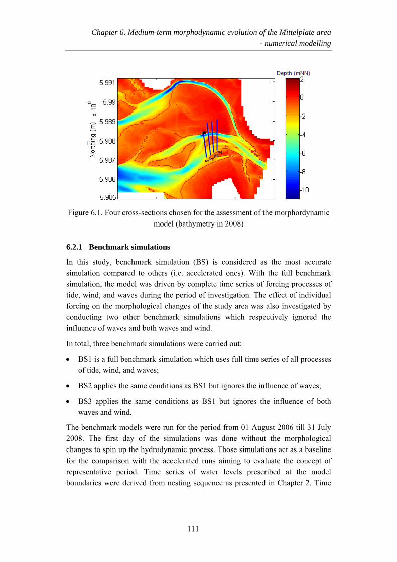
Chapter 6. Medium-term morphodynamic evolution of the Mittelplate area - numerical modelling
4
Figure 6.1. Four cross-sections chosen fmodel (bathy
6.2.1 Benchmark simulations
In this study, benchmark simulation (simulation compared to others (i.e. accsimulation, the model was driven by cotide, wind, and waves during the periodforcing on the morphological changes oconducting two other benchmark siminfluence of waves and both waves and w
In total, three benchmark simulations we
• BS1 is a full benchmark simulation wof tide, wind, and waves;
• BS2 applies the same conditions as B
• BS3 applies the same conditions awaves and wind.
The benchmark models were run for the2008. The first day of the simulationchanges to spin up the hydrodynamic prfor the comparison with the acceleraterepresentative period. Time series ofboundaries were derived from nesting s
11
P1
P
or themetry
BS) elera
mple of inf theulatio
ind.
re ca
hich
S1 b
s BS
peris waocessd run wateque
1
P P2
3
assessment of the morphordynamic in 2008)
is considered as the most accurate ted ones). With the full benchmark te time series of forcing processes of vestigation. The effect of individual study area was also investigated by ns which respectively ignored the
rried out:
uses full time series of all processes
ut ignores the influence of waves;
1 but ignores the influence of both
od from 01 August 2006 till 31 July s done without the morphological . Those simulations act as a baseline s aiming to evaluate the concept of er levels prescribed at the model nce as presented in Chapter 2. Time
Chapter 6. Medium-term morphodynamic evolution of the Mittelplate area - numerical modelling
series of spatial varying wind forcing and pressure were taken from meteorological time series provided by DWD. Swell waves arrived to the model area were obtained by nesting the Mittelplate Model to German Bight Model, which were assigned constantly along the boundaries of the wave model.
6.2.2 Accelerated simulations
Accelerated Simulations (AS) made use of the same process models of hydrodynamic, wave, and sediment transport as used for the benchmark runs. It was decided to select 10 one-month representative periods to perform the simulations for testing the methods. The selection of these representative periods is presented in subsequent section. As the result, fMOR of 24 was applied to cover the two-year simulation period. It means that the modelled bed level change at each hydrodynamic time step is multiplied by the factor 24. Wind and pressure fields within the respective representative period were obtained from PRISMA or COSMO model. Water levels and swell waves prescribed along the boundaries of the flow and wave models resulted from nesting procedure.
Similar to the case of benchmark runs, accelerated simulations considering the effects of:
a) tide
b) tide and wind
c) tide, wind and waves
were performed with the same settings used in the benchmark runs. In total, a series of 30 accelerated model runs were carried out and were coded as:
• AS01.RP01, AS02.RP02, …AS10.RP10 (case c);
• AS11.RP01, AS12.RP02, …AS20.RP10 (case b) and
• AS21.RP01, AS22.RP02, …AS30.RP10 (case a).
Of which RP01…RP10 stand for Representative Periods 01...10; AS01…AS30 stand for Accelerated Simulations running over a duration of one-month RP which consider all forcing (AS01…AS10), tide and wind (AS11…AS20), and only tide (AS21…AS30). Extra one-day simulation was executed prior the one-month periods without the morphological changes in order to spin up the hydrodynamics.
112
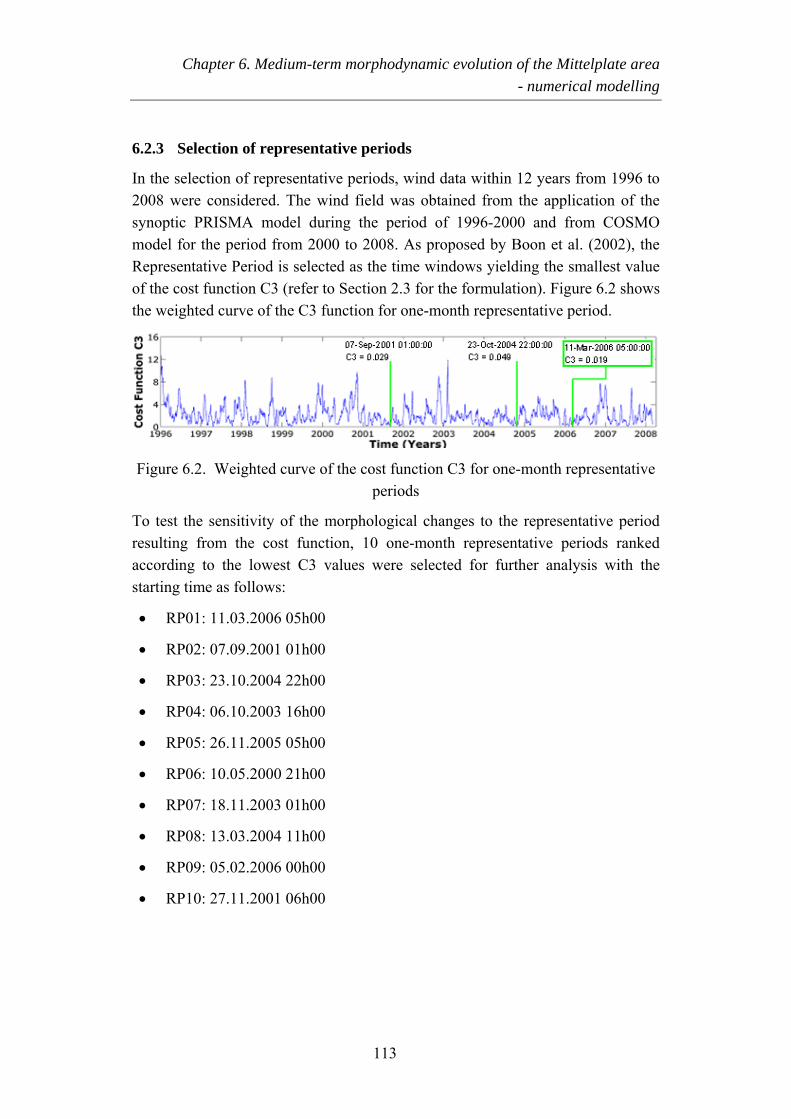
Chapter 6. Medium-term morphodynamic evolution of the Mittelplate area - numerical modelling
6.2.3 Selection of representative periods
In the selection of representative periods, wind data within 12 years from 1996 to 2008 were considered. The wind field was obtained from the application of the synoptic PRISMA model during the period of 1996-2000 and from COSMO model for the period from 2000 to 2008. As proposed by Boon et al. (2002), the Representative Period is selected as the time windows yielding the smallest value of the cost function C3 (refer to Section 2.3 for the formulation). Figure 6.2 shows the weighted curve of the C3 function for one-month representative period.
Figure 6.2. Weighted curve of the cost function C3 for one-month representative periods
To test the sensitivity of the morphological changes to the representative period resulting from the cost function, 10 one-month representative periods ranked according to the lowest C3 values were selected for further analysis with the starting time as follows:
• RP01: 11.03.2006 05h00
• RP02: 07.09.2001 01h00
• RP03: 23.10.2004 22h00
• RP04: 06.10.2003 16h00
• RP05: 26.11.2005 05h00
• RP06: 10.05.2000 21h00
• RP07: 18.11.2003 01h00
• RP08: 13.03.2004 11h00
• RP09: 05.02.2006 00h00
• RP10: 27.11.2001 06h00
113
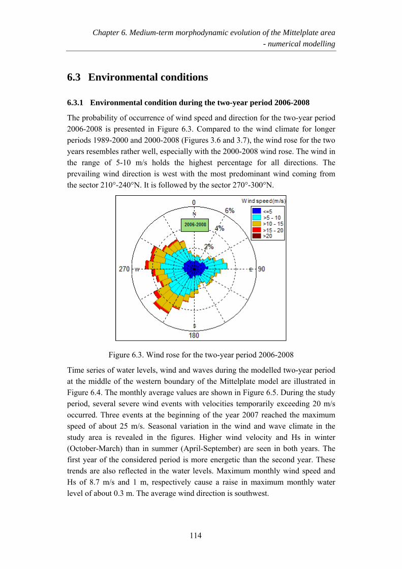
Chapter 6. Medium-term morphodynamic evolution of the Mittelplate area - numerical modelling
6.3 Environmental conditions
6.3.1 Environmental condition during the two-year period 2006-2008
The probability of occurrence of wind speed and direction for the two-year period 2006-2008 is presented in Figure 6.3. Compared to the wind climate for longer periods 1989-2000 and 2000-2008 (Figures 3.6 and 3.7), the wind rose for the two years resembles rather well, especially with the 2000-2008 wind rose. The wind in the range of 5-10 m/s holds the highest percentage for all directions. The prevailing wind direction is west with the most predominant wind coming from the sector 210°-240°N. It is followed by the sector 270°-300°N.
Figure 6.3. Wind rose for the two-year period 2006-2008
Time series of water levels, wind and waves during the modelled two-year period at the middle of the western boundary of the Mittelplate model are illustrated in Figure 6.4. The monthly average values are shown in Figure 6.5. During the study period, several severe wind events with velocities temporarily exceeding 20 m/s occurred. Three events at the beginning of the year 2007 reached the maximum speed of about 25 m/s. Seasonal variation in the wind and wave climate in the study area is revealed in the figures. Higher wind velocity and Hs in winter (October-March) than in summer (April-September) are seen in both years. The first year of the considered period is more energetic than the second year. These trends are also reflected in the water levels. Maximum monthly wind speed and Hs of 8.7 m/s and 1 m, respectively cause a raise in maximum monthly water level of about 0.3 m. The average wind direction is southwest.
114
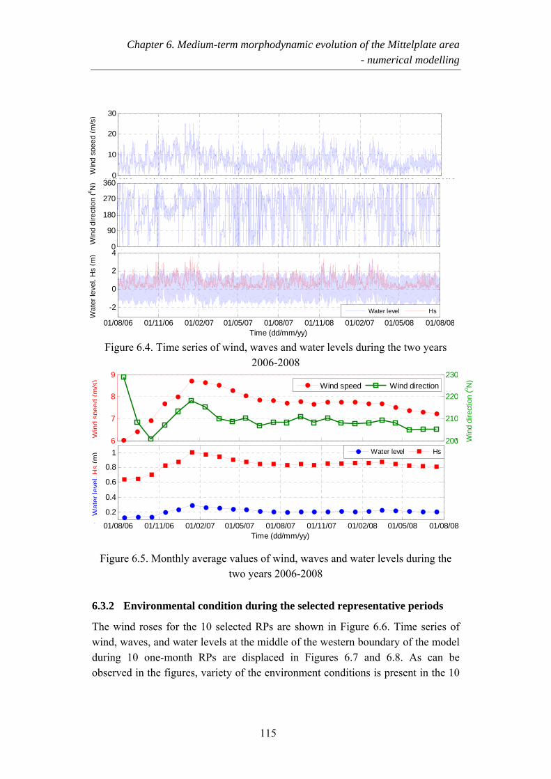
Chapter 6. Medium-term morphodynamic evolution of the Mittelplate area - numerical modelling
01/08/06 01/11/06 01/02/07 01/05/07 01/08/07 01/11/08 01/02/07 01/05/08 01/08/080
10
20
30
Wndspeed(m/s)
01/08/06 01/11/06 01/02/07 01/05/07 01/08/07 01/11/08 01/02/07 01/05/08 01/08/080
90
180
270
360
Wnddrecon
01/08/06 01/11/06 01/02/07 01/05/07 01/08/07 01/11/08 01/02/07 01/05/08 01/08/08
-2
0
2
4
Time (dd/mm/yy)Waterlevel,Hs(m)
Water level Hs
W
ater
leve
l, H
s (m
)
Win
d di
rect
ion
(0 N)
Win
d sp
eed
(m/s
)
Figure 6.4. Time series of wind, waves and water levels during the two years 2006-2008
6
7
8
9
Wind speed (m/s)
/ / / / / / / / / / / / / / / / / /200
210
220
230
W
Wind speed Wind direction
01/08/06 01/11/06 01/02/07 01/05/07 01/08/07 01/11/07 01/02/08 01/05/08 01/08/08
0.2
0.4
0.6
0.8
1
Time (dd/mm/yy)
Waterlevel,Hs(m)
Wat
erle
vel,
Hs
(m)
Win
dsp
eed
(m/s
)
W
ind
dire
ctio
n (0 N
)
Water level Hs
Figure 6.5. Monthly average values of wind, waves and water levels during the
two years 2006-2008
6.3.2 Environmental condition during the selected representative periods
The wind roses for the 10 selected RPs are shown in Figure 6.6. Time series of wind, waves, and water levels at the middle of the western boundary of the model during 10 one-month RPs are displaced in Figures 6.7 and 6.8. As can be observed in the figures, variety of the environment conditions is present in the 10
115
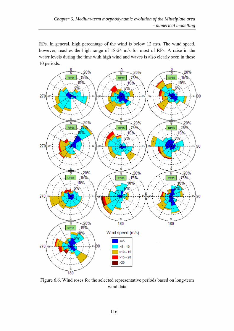
Chapter 6. Medium-term morphodynamic evolution of the Mittelplate area - numerical modelling
RPs. In general, high percentage of the wind is below 12 m/s. The wind speed, however, reaches the high range of 18-24 m/s for most of RPs. A raise in the water levels during the time with high wind and waves is also clearly seen in these 10 periods.
Figure 6.6. Wind roses for the selected representative periods based on long-term
wind data
116
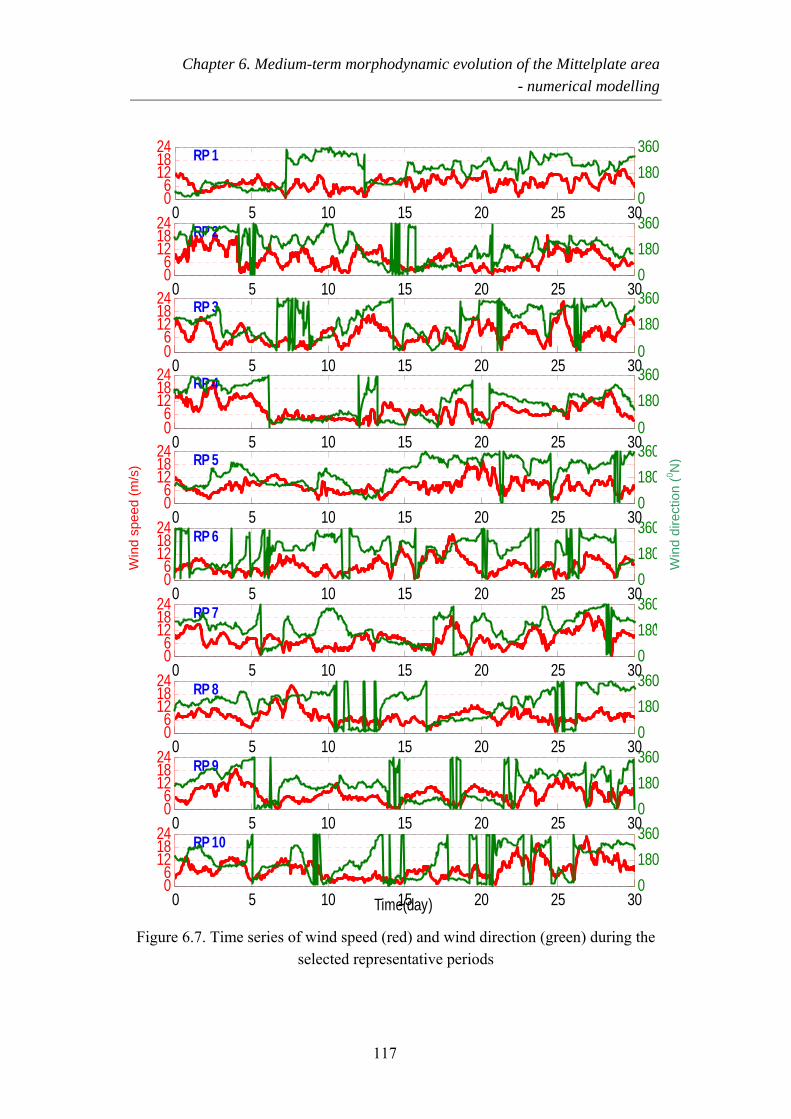
Chapter 6. Medium-term morphodynamic evolution of the Mittelplate area - numerical modelling
06
121824 RP 1
0 5 10 15 20 25 300180360
06
121824 RP 2
0 5 10 15 20 25 300180360
06
121824 RP 3
0 5 10 15 20 25 300180360
06
121824 RP 4
0 5 10 15 20 25 300180360
06
121824 RP 5
0 5 10 15 20 25 300180360
06
121824 RP 6
Windspeed(m/s)
Win
d sp
eed
(m/s
)
0 5 10 15 20 25 300180360
Wind direction (°)
06
121824 RP 7
0 5 10 15 20 25 300180360
Win
d di
rect
ion
(0 N)
06
121824 RP 8
0 5 10 15 20 25 300180360
06
121824 RP 9
0 5 10 15 20 25 300180360
06
121824 RP 10
Time(day)0 5 10 15 20 25 300180360
Figure 6.7. Time series of wind speed (red) and wind direction (green) during the
selected representative periods
117
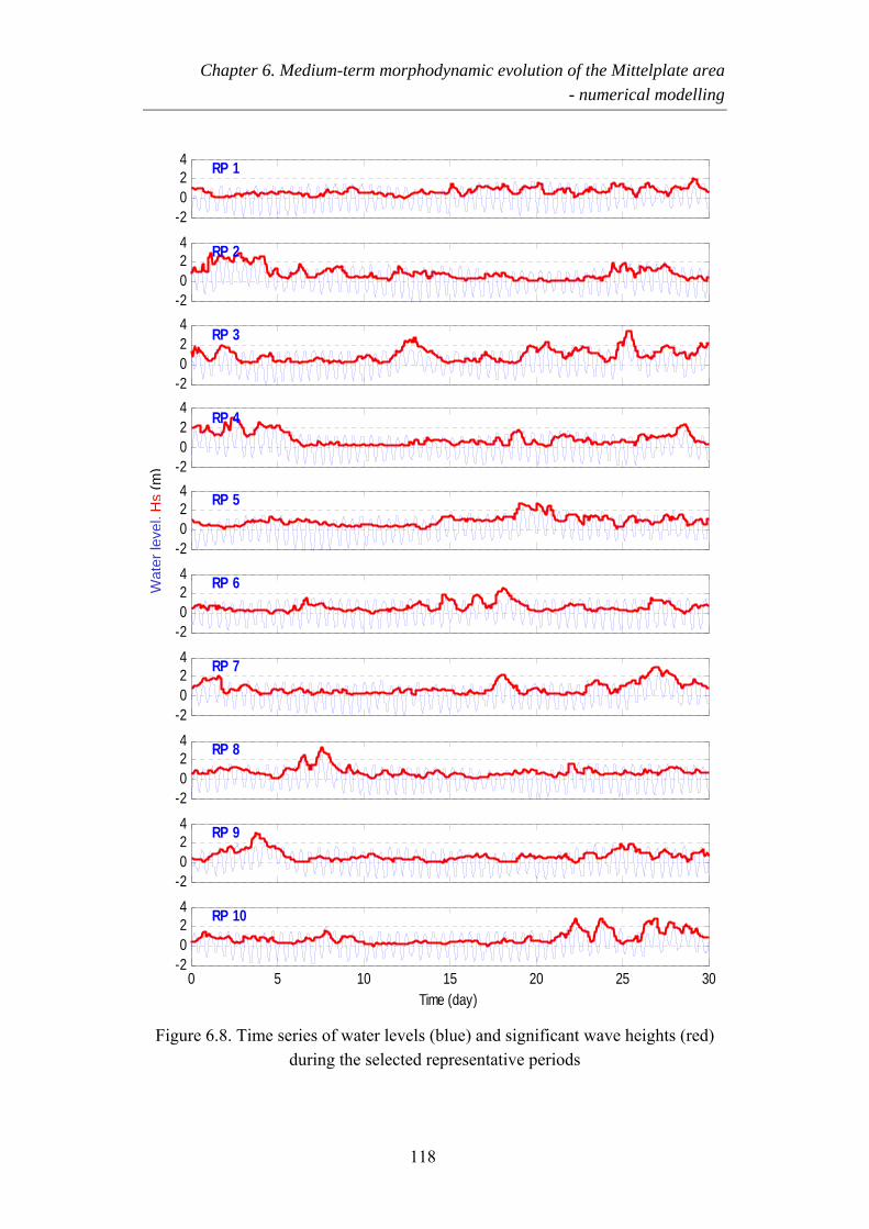
Chapter 6. Medium-term morphodynamic evolution of the Mittelplate area - numerical modelling
-2024 RP 1
-2024 RP 2
-2024 RP 3
-2024 RP 4
-2024 RP 5
Hs,Wtraelevel(
m)
W
ater
leve
l, H
s (m
)
-2024 RP 6
-2024 RP 7
-2024 RP 8
-2024 RP 9
0 5 10 15 20 25 30-2024 RP 10
Time (day) Figure 6.8. Time series of water levels (blue) and significant wave heights (red)
during the selected representative periods
118
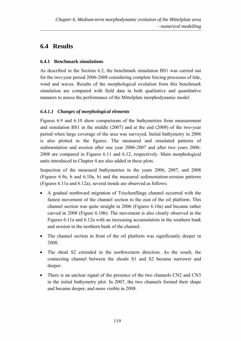
Chapter 6. Medium-term morphodynamic evolution of the Mittelplate area - numerical modelling
6.4 Results
6.4.1 Benchmark simulations
As described in the Section 6.2, the benchmark simulation BS1 was carried out for the two-year period 2006-2008 considering complete forcing processes of tide, wind and waves. Results of the morphological evolution from this benchmark simulation are compared with field data in both qualitative and quantitative manners to assess the performance of the Mittelplate morphodynamic model.
6.4.1.1 Changes of morphological elements
Figures 6.9 and 6.10 show comparisons of the bathymetries from measurement and simulation BS1 in the middle (2007) and at the end (2008) of the two-year period when large coverage of the area was surveyed. Initial bathymetry in 2006 is also plotted in the figures. The measured and simulated patterns of sedimentation and erosion after one year 2006-2007 and after two years 2006-2008 are compared in Figures 6.11 and 6.12, respectively. Main morphological units introduced in Chapter 4 are also added in these plots.
Inspection of the measured bathymetries in the years 2006, 2007, and 2008 (Figures 6.9a, b and 6.10a, b) and the measured sedimentation-erosion patterns (Figures 6.11a and 6.12a), several trends are observed as follows:
• A gradual northward migration of Trischenflinge channel occurred with the fastest movement of the channel section to the east of the oil platform. This channel section was quite straight in 2006 (Figures 6.10a) and became rather curved in 2008 (Figure 6.10b). The movement is also clearly observed in the Figures 6.11a and 6.12a with an increasing accumulation in the southern bank and erosion in the northern bank of the channel.
• The channel section in front of the oil platform was significantly deeper in 2008.
• The shoal S2 extended in the northwestern direction. As the result, the connecting channel between the shoals S1 and S2 became narrower and deeper.
• There is an unclear signal of the presence of the two channels CN2 and CN3 in the initial bathymetry plot. In 2007, the two channels formed their shape and became deeper, and more visible in 2008.
119
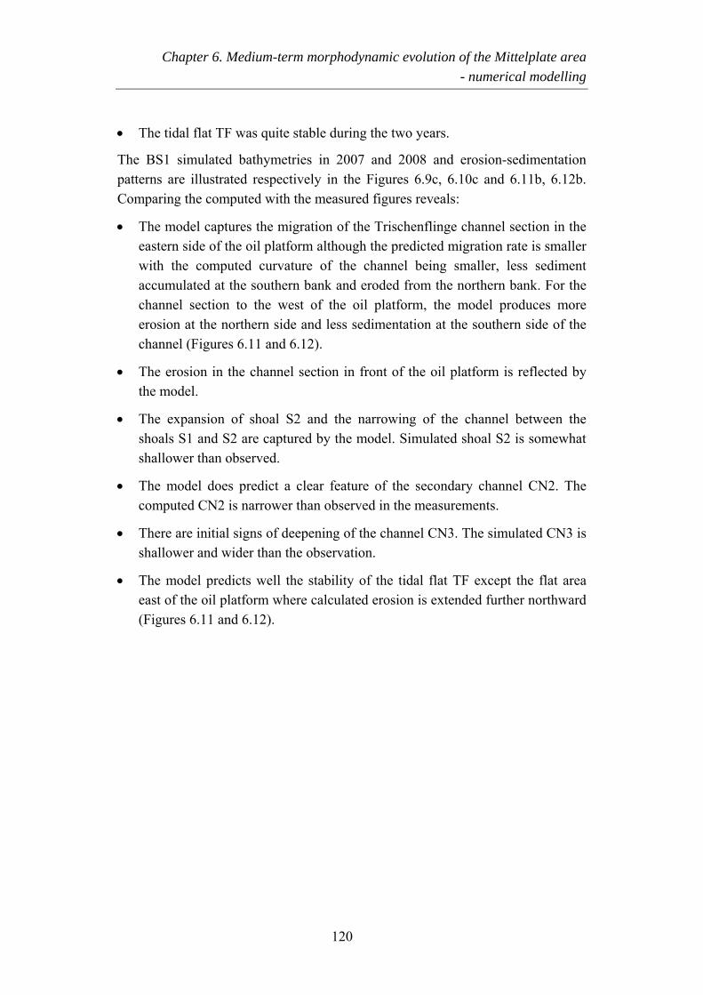
Chapter 6. Medium-term morphodynamic evolution of the Mittelplate area - numerical modelling
• The tidal flat TF was quite stable during the two years.
The BS1 simulated bathymetries in 2007 and 2008 and erosion-sedimentation patterns are illustrated respectively in the Figures 6.9c, 6.10c and 6.11b, 6.12b. Comparing the computed with the measured figures reveals:
• The model captures the migration of the Trischenflinge channel section in the eastern side of the oil platform although the predicted migration rate is smaller with the computed curvature of the channel being smaller, less sediment accumulated at the southern bank and eroded from the northern bank. For the channel section to the west of the oil platform, the model produces more erosion at the northern side and less sedimentation at the southern side of the channel (Figures 6.11 and 6.12).
• The erosion in the channel section in front of the oil platform is reflected by the model.
• The expansion of shoal S2 and the narrowing of the channel between the shoals S1 and S2 are captured by the model. Simulated shoal S2 is somewhat shallower than observed.
• The model does predict a clear feature of the secondary channel CN2. The computed CN2 is narrower than observed in the measurements.
• There are initial signs of deepening of the channel CN3. The simulated CN3 is shallower and wider than the observation.
• The model predicts well the stability of the tidal flat TF except the flat area east of the oil platform where calculated erosion is extended further northward (Figures 6.11 and 6.12).
120
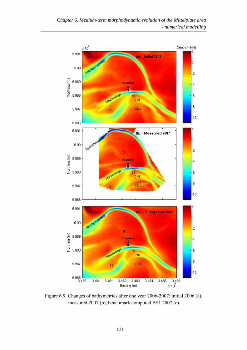
Chapter 6. Medium-term morphodynamic evolution of the Mittelplate area - numerical modelling
Figure 6.9. Changes of bathymetries after one year 2006-2007: initial 2006 (a), measured 2007 (b), benchmark computed BS1 2007 (c)
121
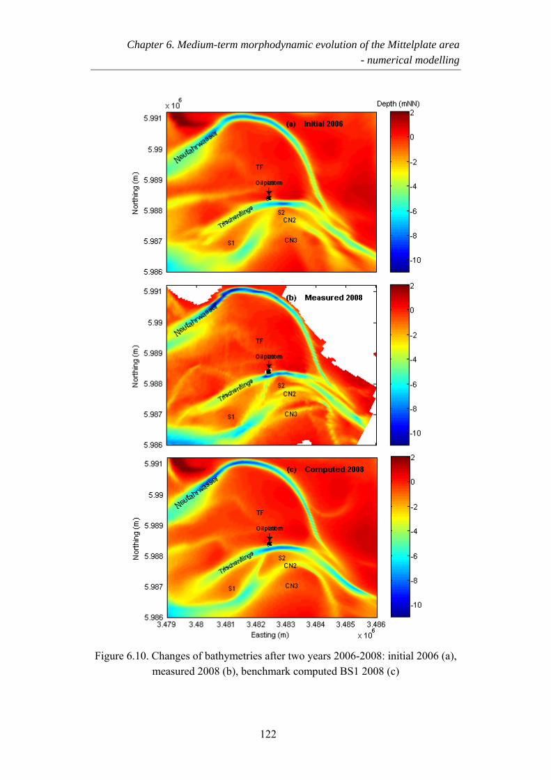
Chapter 6. Medium-term morphodynamic evolution of the Mittelplate area - numerical modelling
Figure 6.10. Changes of bathymetries after two years 2006-2008: initial 2006 (a), measured 2008 (b), benchmark computed BS1 2008 (c)
122
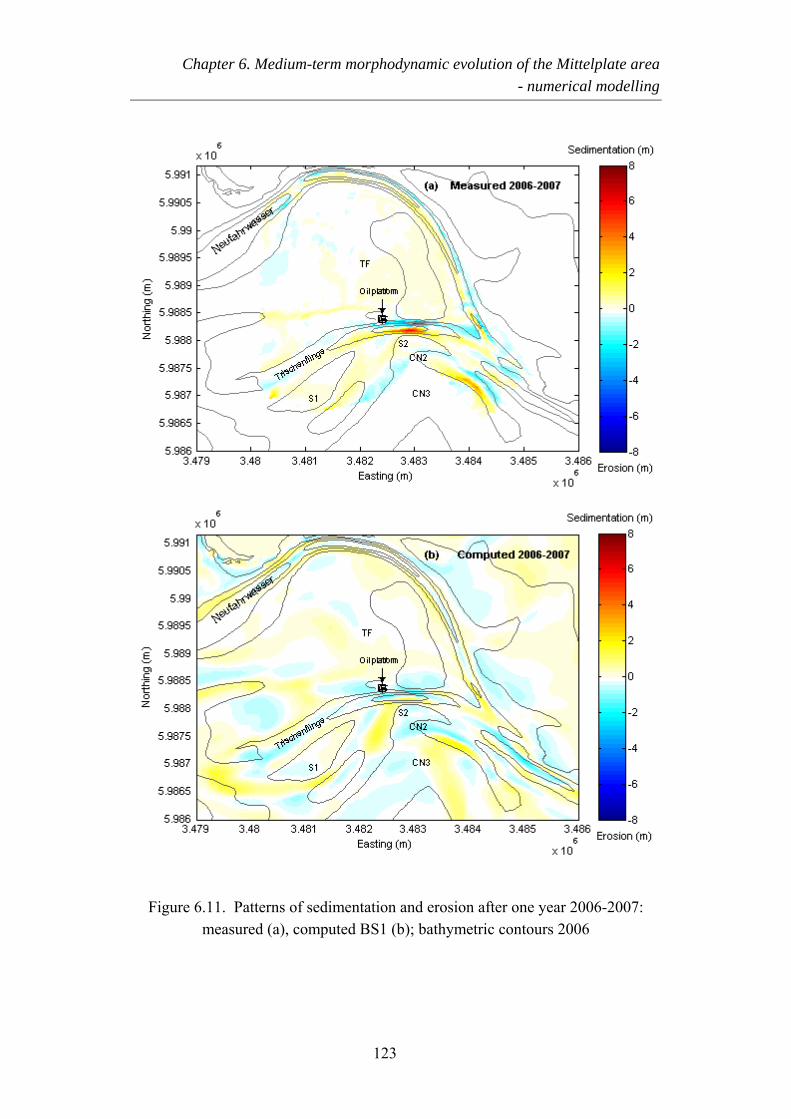
Chapter 6. Medium-term morphodynamic evolution of the Mittelplate area - numerical modelling
Figure 6.11. Patterns of sedimentation and erosion after one year 2006-2007:
measured (a), computed BS1 (b); bathymetric contours 2006
123
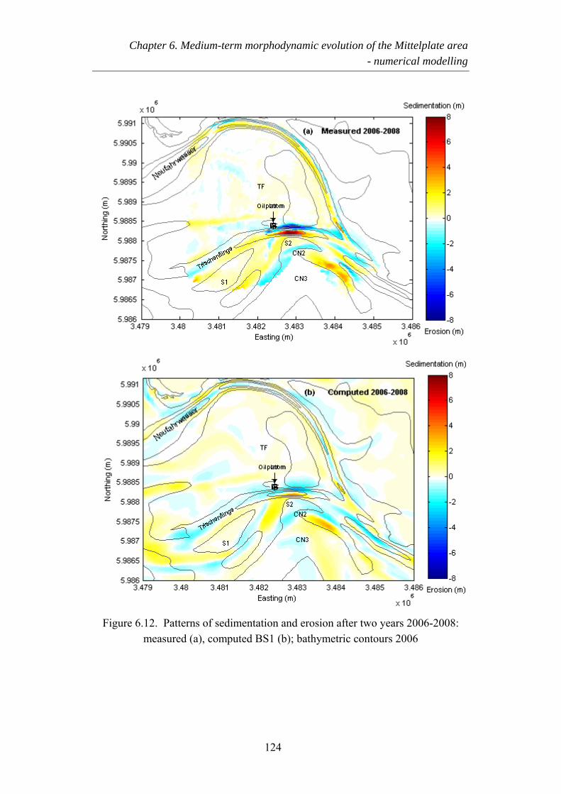
Chapter 6. Medium-term morphodynamic evolution of the Mittelplate area - numerical modelling
Figure 6.12. Patterns of sedimentation and erosion after two years 2006-2008: measured (a), computed BS1 (b); bathymetric contours 2006
124
Chapter 6. Medium-term morphodynamic evolution of the Mittelplate area - numerical modelling
6.4.1.2 Changes of channel cross-sections
The ability of the morphodynamic benchmark modelling in describing the morphological changes is also assessed on the base of four cross-sections Pl, P2, P3, and P4 as indicated in Figure 6.1. The evaluation is done for the two time points: in the middle and at the end of the study period in 06.2007 and 07.2008, respectively (Figures 6.13 and 6.14). Some of the local, small-scale features of the measured channel cross-sections are not visible because the model grid is too coarse to display the details. For example, the two sub-channels in front of the oil platform in 2008, which were discussed in Chapter 4, are not visible in the following plots. With regard to the result from simulation BS1, the gradual migration of the Trischenflinge is reflected in all selected cross-sections. However, the predicted migration rate is lower than the observation. The deepening of the tidal channel at cross-section P1 is reasonably well captured at the end of the simulation but is overestimated for the year 2007. The shallow secondary channel CN2 is clearly visible. It is deeper than observed for P3 and P4 in the year 2007. Quantitatively, the BSS value is slightly higher for the one-year period 2006-2007 than for the two years 2006-2008 for all cross-sections, except P1. Generally, the model is rated as good for almost the cases according to the classification of Van Rijn et al. (2003), except for cross-sections P1 and P3 in the year 2007, which are qualified as fair and excellent, respectively.
125
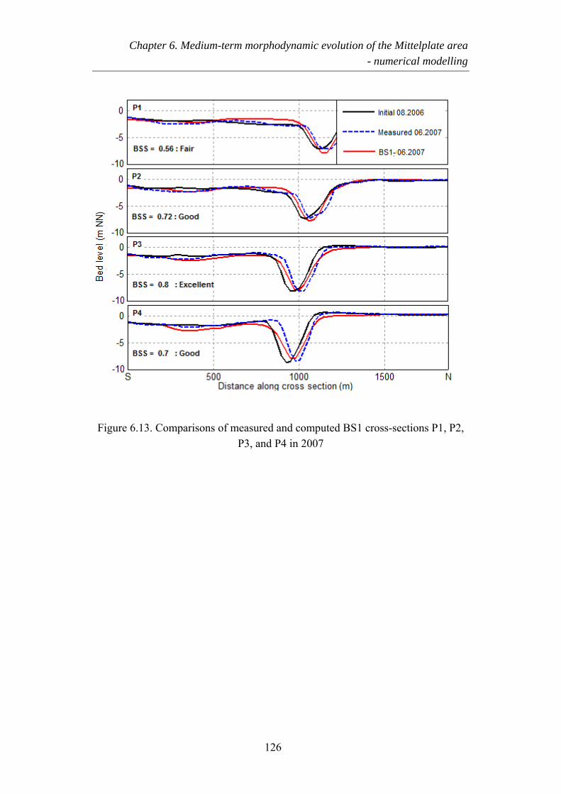
Chapter 6. Medium-term morphodynamic evolution of the Mittelplate area - numerical modelling
Figure 6.13. Comparisons of measured and computed BS1 cross-sections P1, P2, P3, and P4 in 2007
126
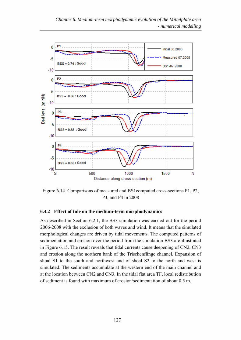
Chapter 6. Medium-term morphodynamic evolution of the Mittelplate area - numerical modelling
Figure 6.14. Comparisons of measured and BS1computed cross-sections P1, P2, P3, and P4 in 2008
6.4.2 Effect of tide on the medium-term morphodynamics
As described in Section 6.2.1, the BS3 simulation was carried out for the period 2006-2008 with the exclusion of both waves and wind. It means that the simulated morphological changes are driven by tidal movements. The computed patterns of sedimentation and erosion over the period from the simulation BS3 are illustrated in Figure 6.15. The result reveals that tidal currents cause deepening of CN2, CN3 and erosion along the northern bank of the Trischenflinge channel. Expansion of shoal S1 to the south and northwest and of shoal S2 to the north and west is simulated. The sediments accumulate at the western end of the main channel and at the location between CN2 and CN3. In the tidal flat area TF, local redistribution of sediment is found with maximum of erosion/sedimentation of about 0.5 m.
127
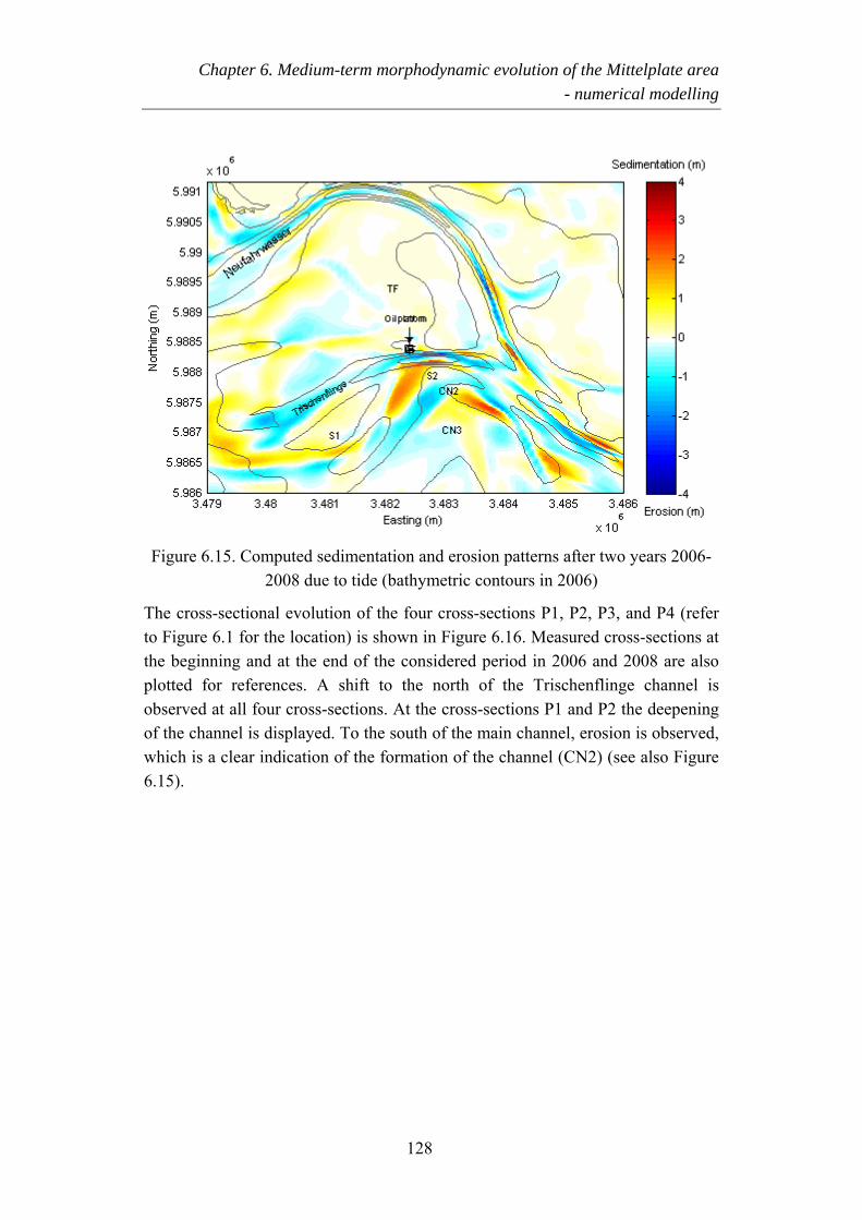
Chapter 6. Medium-term morphodynamic evolution of the Mittelplate area - numerical modelling
Figure 6.15. Computed sedimentation and erosion patterns after two years 2006-2008 due to tide (bathymetric contours in 2006)
The cross-sectional evolution of the four cross-sections P1, P2, P3, and P4 (refer to Figure 6.1 for the location) is shown in Figure 6.16. Measured cross-sections at the beginning and at the end of the considered period in 2006 and 2008 are also plotted for references. A shift to the north of the Trischenflinge channel is observed at all four cross-sections. At the cross-sections P1 and P2 the deepening of the channel is displayed. To the south of the main channel, erosion is observed, which is a clear indication of the formation of the channel (CN2) (see also Figure 6.15).
128
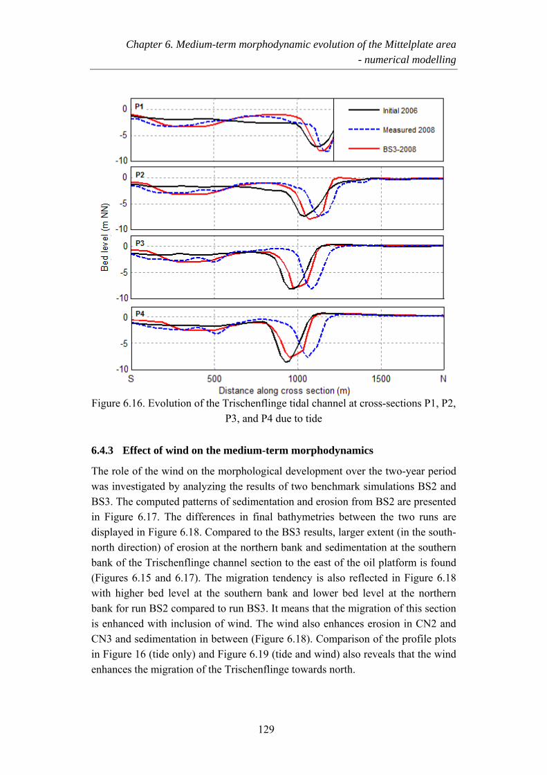
Chapter 6. Medium-term morphodynamic evolution of the Mittelplate area - numerical modelling
Figure 6.16. Evolution of the Trischenflinge tidal channel at cross-sections P1, P2,
P3, and P4 due to tide
6.4.3 Effect of wind on the medium-term morphodynamics
The role of the wind on the morphological development over the two-year period was investigated by analyzing the results of two benchmark simulations BS2 and BS3. The computed patterns of sedimentation and erosion from BS2 are presented in Figure 6.17. The differences in final bathymetries between the two runs are displayed in Figure 6.18. Compared to the BS3 results, larger extent (in the south-north direction) of erosion at the northern bank and sedimentation at the southern bank of the Trischenflinge channel section to the east of the oil platform is found (Figures 6.15 and 6.17). The migration tendency is also reflected in Figure 6.18 with higher bed level at the southern bank and lower bed level at the northern bank for run BS2 compared to run BS3. It means that the migration of this section is enhanced with inclusion of wind. The wind also enhances erosion in CN2 and CN3 and sedimentation in between (Figure 6.18). Comparison of the profile plots in Figure 16 (tide only) and Figure 6.19 (tide and wind) also reveals that the wind enhances the migration of the Trischenflinge towards north.
129
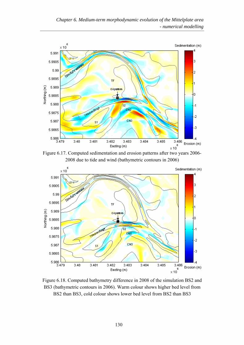
Chapter 6. Medium-term morphodynamic evolution of the Mittelplate area - numerical modelling
Figure 6.17. Computed sedimentation and erosion patterns after two years 2006-
2008 due to tide and wind (bathymetric contours in 2006)
Figure 6.18. Computed bathymetry difference in 2008 of the simulation BS2 and BS3 (bathymetric contours in 2006). Warm colour shows higher bed level from
BS2 than BS3, cold colour shows lower bed level from BS2 than BS3
130
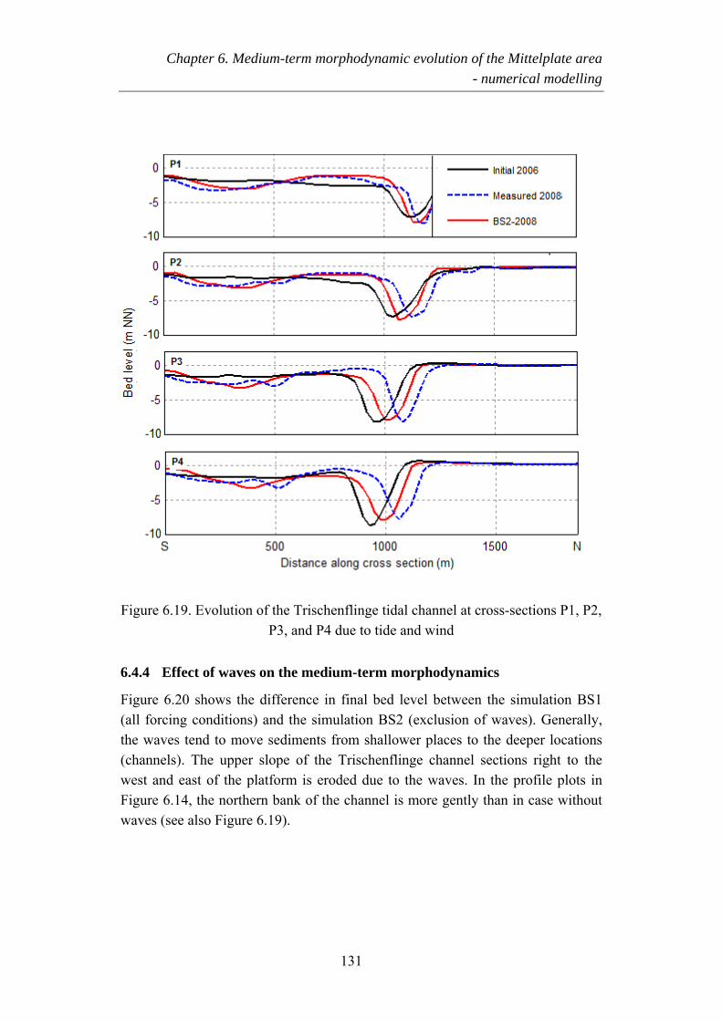
Chapter 6. Medium-term morphodynamic evolution of the Mittelplate area - numerical modelling
Figure 6.19. Evolution of the Trischenflinge tidal channel at cross-sections P1, P2,
P3, and P4 due to tide and wind
6.4.4 Effect of waves on the medium-term morphodynamics
Figure 6.20 shows the difference in final bed level between the simulation BS1 (all forcing conditions) and the simulation BS2 (exclusion of waves). Generally, the waves tend to move sediments from shallower places to the deeper locations (channels). The upper slope of the Trischenflinge channel sections right to the west and east of the platform is eroded due to the waves. In the profile plots in Figure 6.14, the northern bank of the channel is more gently than in case without waves (see also Figure 6.19).
131
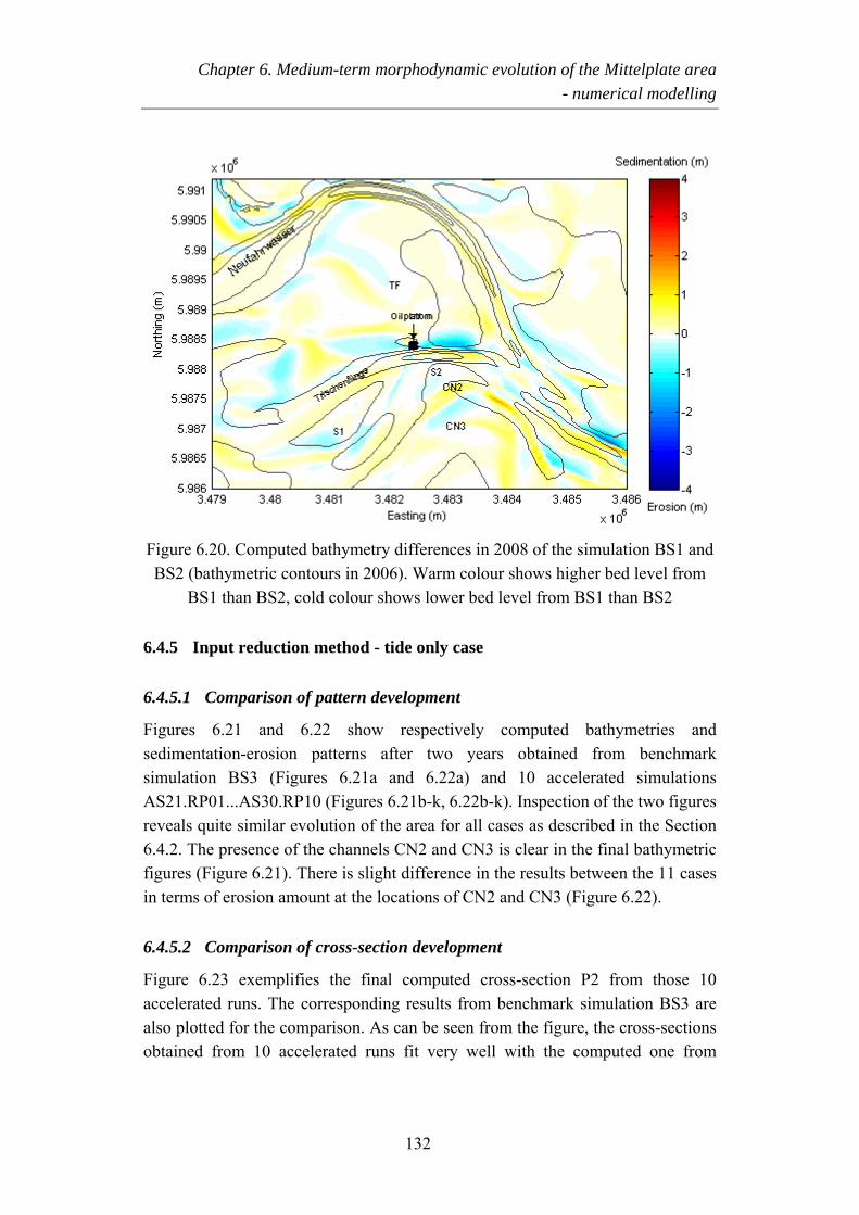
Chapter 6. Medium-term morphodynamic evolution of the Mittelplate area - numerical modelling
Figure 6.20. Computed bathymetry differences in 2008 of the simulation BS1 and BS2 (bathymetric contours in 2006). Warm colour shows higher bed level from
BS1 than BS2, cold colour shows lower bed level from BS1 than BS2
6.4.5 Input reduction method - tide only case
6.4.5.1 Comparison of pattern development
Figures 6.21 and 6.22 show respectively computed bathymetries and sedimentation-erosion patterns after two years obtained from benchmark simulation BS3 (Figures 6.21a and 6.22a) and 10 accelerated simulations AS21.RP01...AS30.RP10 (Figures 6.21b-k, 6.22b-k). Inspection of the two figures reveals quite similar evolution of the area for all cases as described in the Section 6.4.2. The presence of the channels CN2 and CN3 is clear in the final bathymetric figures (Figure 6.21). There is slight difference in the results between the 11 cases in terms of erosion amount at the locations of CN2 and CN3 (Figure 6.22).
6.4.5.2 Comparison of cross-section development
Figure 6.23 exemplifies the final computed cross-section P2 from those 10 accelerated runs. The corresponding results from benchmark simulation BS3 are also plotted for the comparison. As can be seen from the figure, the cross-sections obtained from 10 accelerated runs fit very well with the computed one from
132
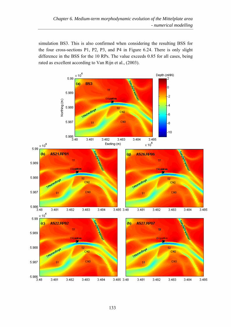
Chapter 6. Medium-term morphodynamic evolution of the Mittelplate area - numerical modelling
simulation BS3. This is also confirmed when considering the resulting BSS for the four cross-sections P1, P2, P3, and P4 in Figure 6.24. There is only slight difference in the BSS for the 10 RPs. The value exceeds 0.85 for all cases, being rated as excellent according to Van Rijn et al., (2003).
133
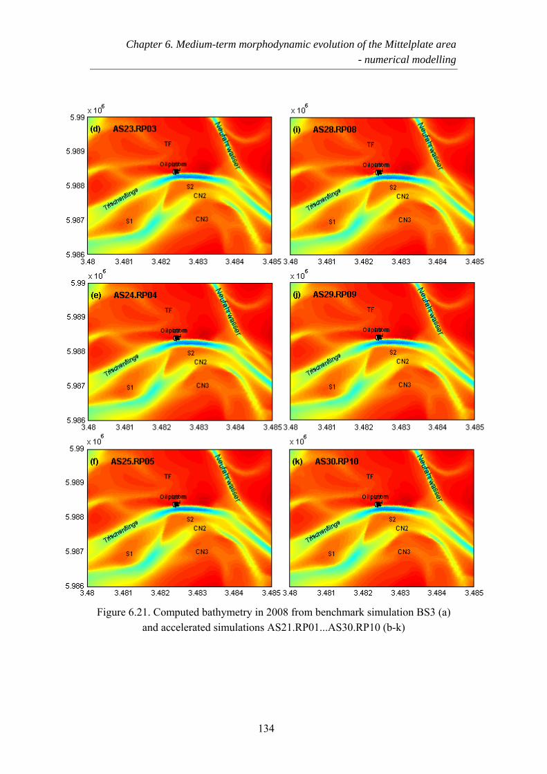
Chapter 6. Medium-term morphodynamic evolution of the Mittelplate area - numerical modelling
Figure 6.21. Computed bathymetry in 2008 from benchmark simulation BS3 (a) and accelerated simulations AS21.RP01...AS30.RP10 (b-k)
134
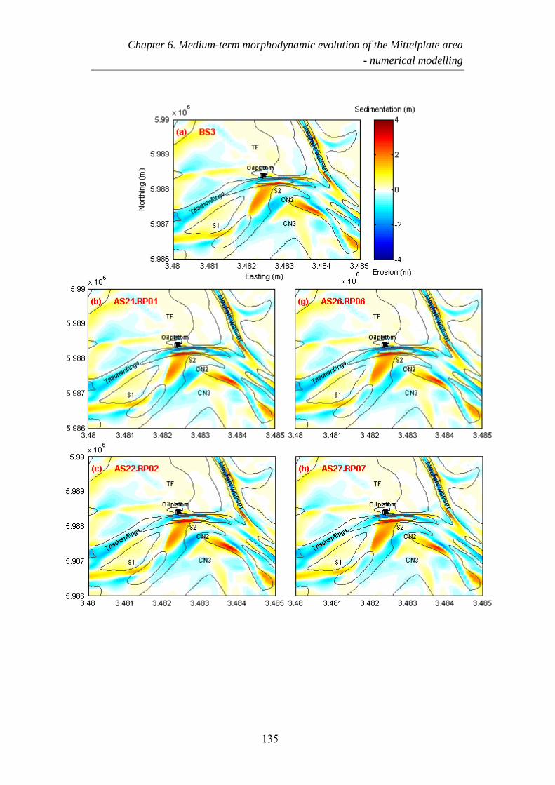
Chapter 6. Medium-term morphodynamic evolution of the Mittelplate area - numerical modelling
135
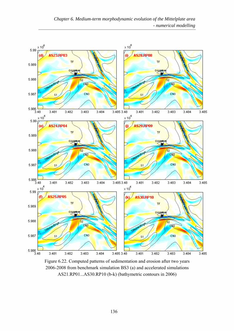
Chapter 6. Medium-term morphodynamic evolution of the Mittelplate area - numerical modelling
Figure 6.22. Computed patterns of sedimentation and erosion after two years 2006-2008 from benchmark simulation BS3 (a) and accelerated simulations
AS21.RP01...AS30.RP10 (b-k) (bathymetric contours in 2006)
136
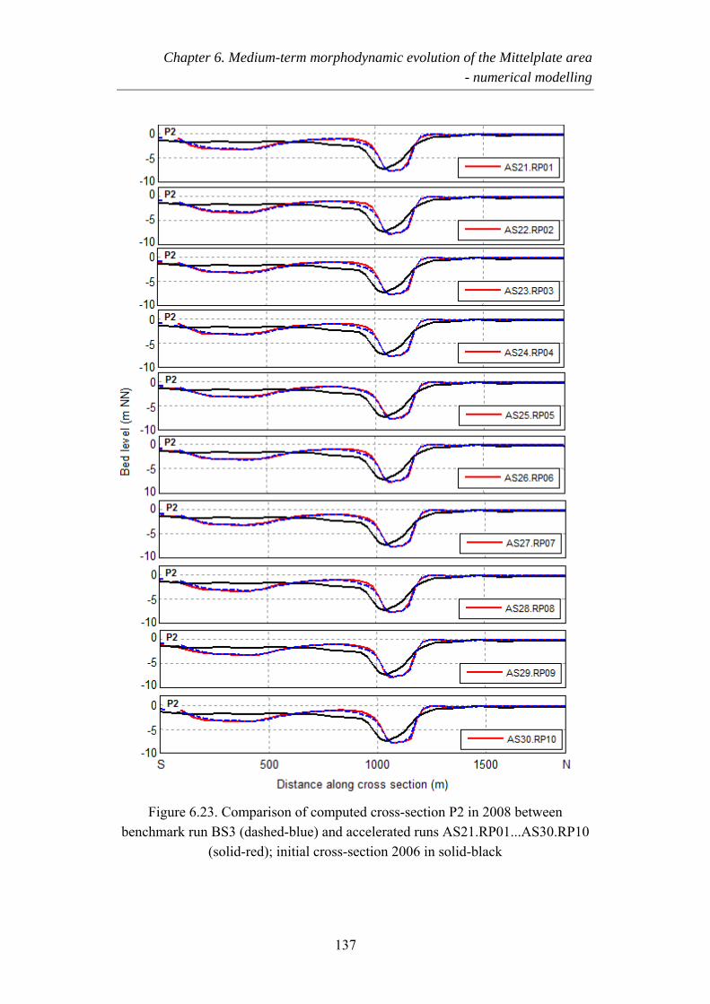
Chapter 6. Medium-term morphodynamic evolution of the Mittelplate area - numerical modelling
Figure 6.23. Comparison of computed cross-section P2 in 2008 between benchmark run BS3 (dashed-blue) and accelerated runs AS21.RP01...AS30.RP10
(solid-red); initial cross-section 2006 in solid-black
137
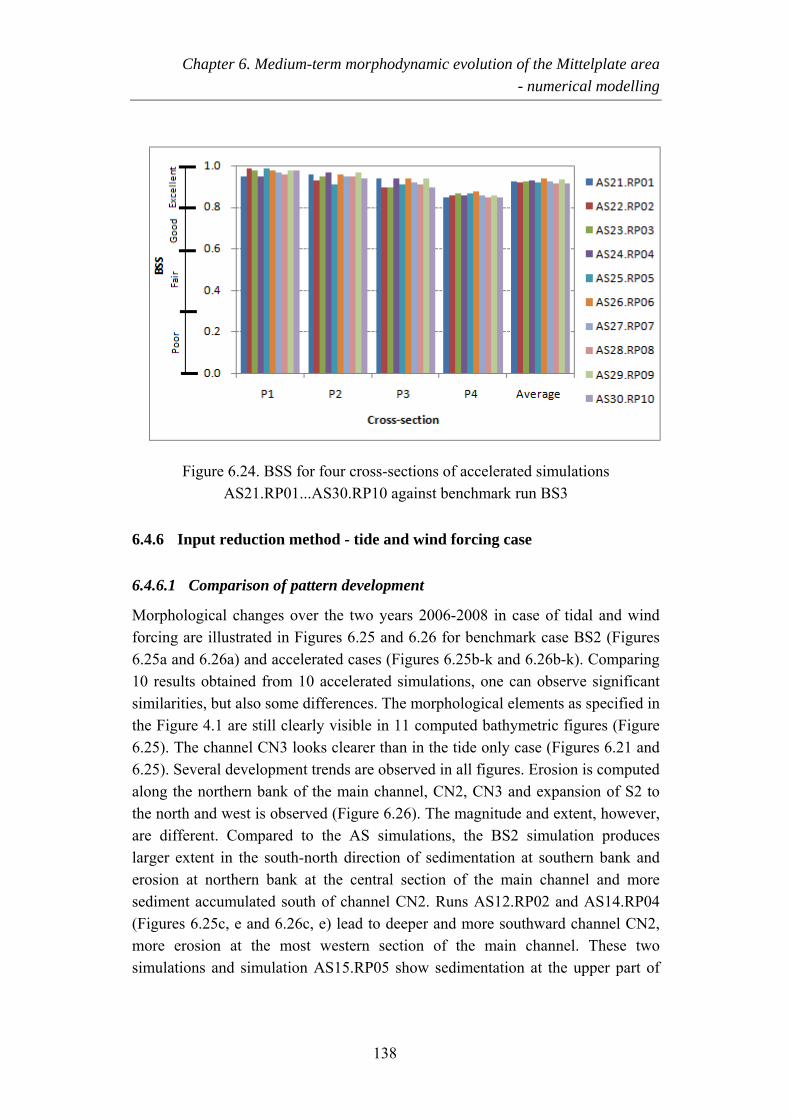
Chapter 6. Medium-term morphodynamic evolution of the Mittelplate area - numerical modelling
Figure 6.24. BSS for four cross-sections of accelerated simulations AS21.RP01...AS30.RP10 against benchmark run BS3
6.4.6 Input reduction method - tide and wind forcing case
6.4.6.1 Comparison of pattern development
Morphological changes over the two years 2006-2008 in case of tidal and wind forcing are illustrated in Figures 6.25 and 6.26 for benchmark case BS2 (Figures 6.25a and 6.26a) and accelerated cases (Figures 6.25b-k and 6.26b-k). Comparing 10 results obtained from 10 accelerated simulations, one can observe significant similarities, but also some differences. The morphological elements as specified in the Figure 4.1 are still clearly visible in 11 computed bathymetric figures (Figure 6.25). The channel CN3 looks clearer than in the tide only case (Figures 6.21 and 6.25). Several development trends are observed in all figures. Erosion is computed along the northern bank of the main channel, CN2, CN3 and expansion of S2 to the north and west is observed (Figure 6.26). The magnitude and extent, however, are different. Compared to the AS simulations, the BS2 simulation produces larger extent in the south-north direction of sedimentation at southern bank and erosion at northern bank at the central section of the main channel and more sediment accumulated south of channel CN2. Runs AS12.RP02 and AS14.RP04 (Figures 6.25c, e and 6.26c, e) lead to deeper and more southward channel CN2, more erosion at the most western section of the main channel. These two simulations and simulation AS15.RP05 show sedimentation at the upper part of
138
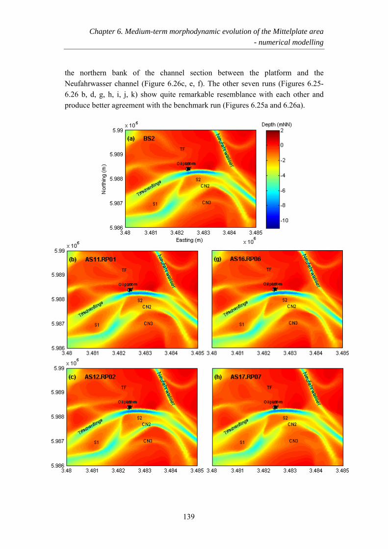
Chapter 6. Medium-term morphodynamic evolution of the Mittelplate area - numerical modelling
the northern bank of the channel section between the platform and the Neufahrwasser channel (Figure 6.26c, e, f). The other seven runs (Figures 6.25-6.26 b, d, g, h, i, j, k) show quite remarkable resemblance with each other and produce better agreement with the benchmark run (Figures 6.25a and 6.26a).
139
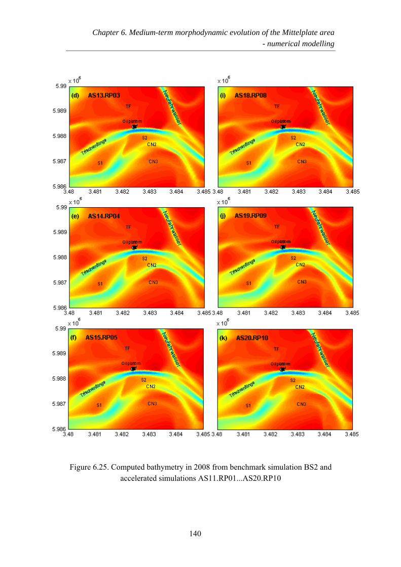
Chapter 6. Medium-term morphodynamic evolution of the Mittelplate area - numerical modelling
Figure 6.25. Computed bathymetry in 2008 from benchmark simulation BS2 and accelerated simulations AS11.RP01...AS20.RP10
140
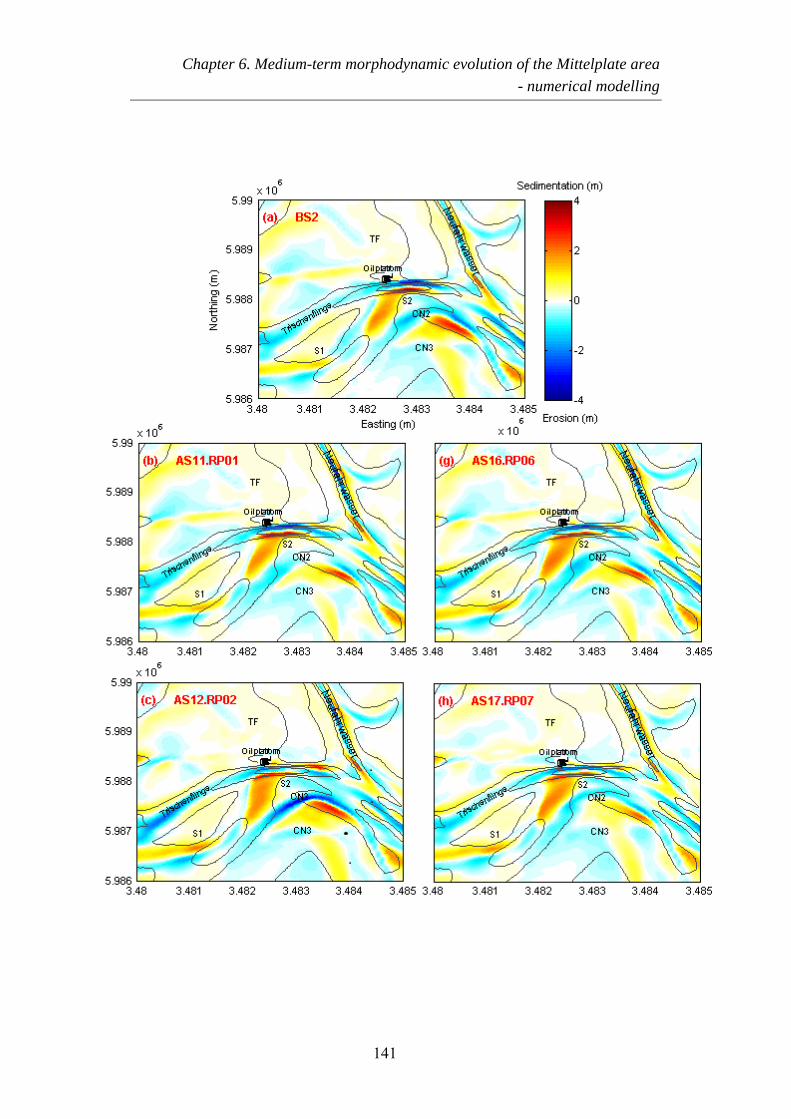
Chapter 6. Medium-term morphodynamic evolution of the Mittelplate area - numerical modelling
141
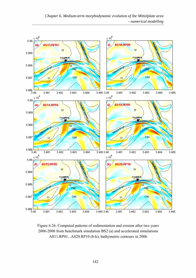
Chapter 6. Medium-term morphodynamic evolution of the Mittelplate area - numerical modelling
Figure 6.26. Computed patterns of sedimentation and erosion after two years 2006-2008 from benchmark simulation BS2 (a) and accelerated simulations
AS11.RP01...AS20.RP10 (b-k); bathymetric contours in 2006
142
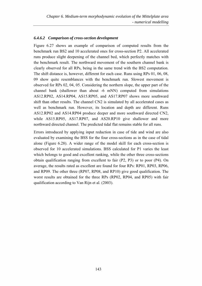
Chapter 6. Medium-term morphodynamic evolution of the Mittelplate area - numerical modelling
6.4.6.2 Comparison of cross-section development
Figure 6.27 shows an example of comparison of computed results from the benchmark run BS2 and 10 accelerated ones for cross-section P2. All accelerated runs produce slight deepening of the channel bed, which perfectly matches with the benchmark result. The northward movement of the southern channel bank is clearly observed for all RPs, being in the same trend with the BS2 computation. The shift distance is, however, different for each case. Runs using RPs 01, 06, 08, 09 show quite resemblances with the benchmark run. Slowest movement is observed for RPs 02, 04, 05. Considering the northern slope, the upper part of the channel bank (shallower than about -6 mNN) computed from simulations AS12.RP02, AS14.RP04, AS15.RP05, and AS17.RP07 shows more southward shift than other results. The channel CN2 is simulated by all accelerated cases as well as benchmark run. However, its location and depth are different. Runs AS12.RP02 and AS14.RP04 produce deeper and more southward directed CN2, while AS15.RP05, AS17.RP07, and AS20.RP10 give shallower and more northward directed channel. The predicted tidal flat remains stable for all runs.
Errors introduced by applying input reduction in case of tide and wind are also evaluated by examining the BSS for the four cross-sections as in the case of tidal alone (Figure 6.28). A wider range of the model skill for each cross-section is observed for 10 accelerated simulations. BSS calculated for P1 varies the least which belongs to good and excellent ranking, while the other three cross-sections obtain qualification ranging from excellent to fair (P2, P3) or to poor (P4). On average, the results rated as excellent are found for four RPs: RP01, RP03, RP06, and RP09. The other three (RP07, RP08, and RP10) give good qualification. The worst results are obtained for the three RPs (RP02, RP04, and RP05) with fair qualification according to Van Rijn et al. (2003).
143
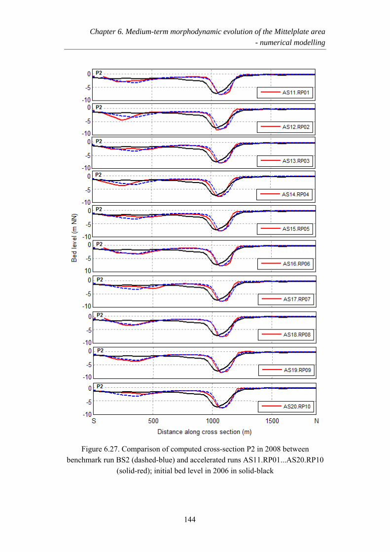
Chapter 6. Medium-term morphodynamic evolution of the Mittelplate area - numerical modelling
Figure 6.27. Comparison of computed cross-section P2 in 2008 between benchmark run BS2 (dashed-blue) and accelerated runs AS11.RP01...AS20.RP10
(solid-red); initial bed level in 2006 in solid-black
144
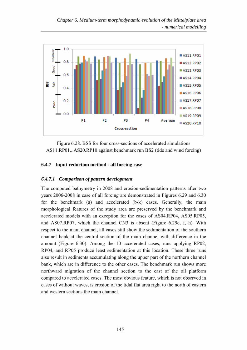
Chapter 6. Medium-term morphodynamic evolution of the Mittelplate area - numerical modelling
Figure 6.28. BSS for four cross-sections of accelerated simulations AS11.RP01...AS20.RP10 against benchmark run BS2 (tide and wind forcing)
6.4.7 Input reduction method - all forcing case
6.4.7.1 Comparison of pattern development
The computed bathymetry in 2008 and erosion-sedimentation patterns after two years 2006-2008 in case of all forcing are demonstrated in Figures 6.29 and 6.30 for the benchmark (a) and accelerated (b-k) cases. Generally, the main morphological features of the study area are preserved by the benchmark and accelerated models with an exception for the cases of AS04.RP04, AS05.RP05, and AS07.RP07, which the channel CN3 is absent (Figure 6.29e, f, h). With respect to the main channel, all cases still show the sedimentation of the southern channel bank at the central section of the main channel with difference in the amount (Figure 6.30). Among the 10 accelerated cases, runs applying RP02, RP04, and RP05 produce least sedimentation at this location. These three runs also result in sediments accumulating along the upper part of the northern channel bank, which are in difference to the other cases. The benchmark run shows more northward migration of the channel section to the east of the oil platform compared to accelerated cases. The most obvious feature, which is not observed in cases of without waves, is erosion of the tidal flat area right to the north of eastern and western sections the main channel.
145
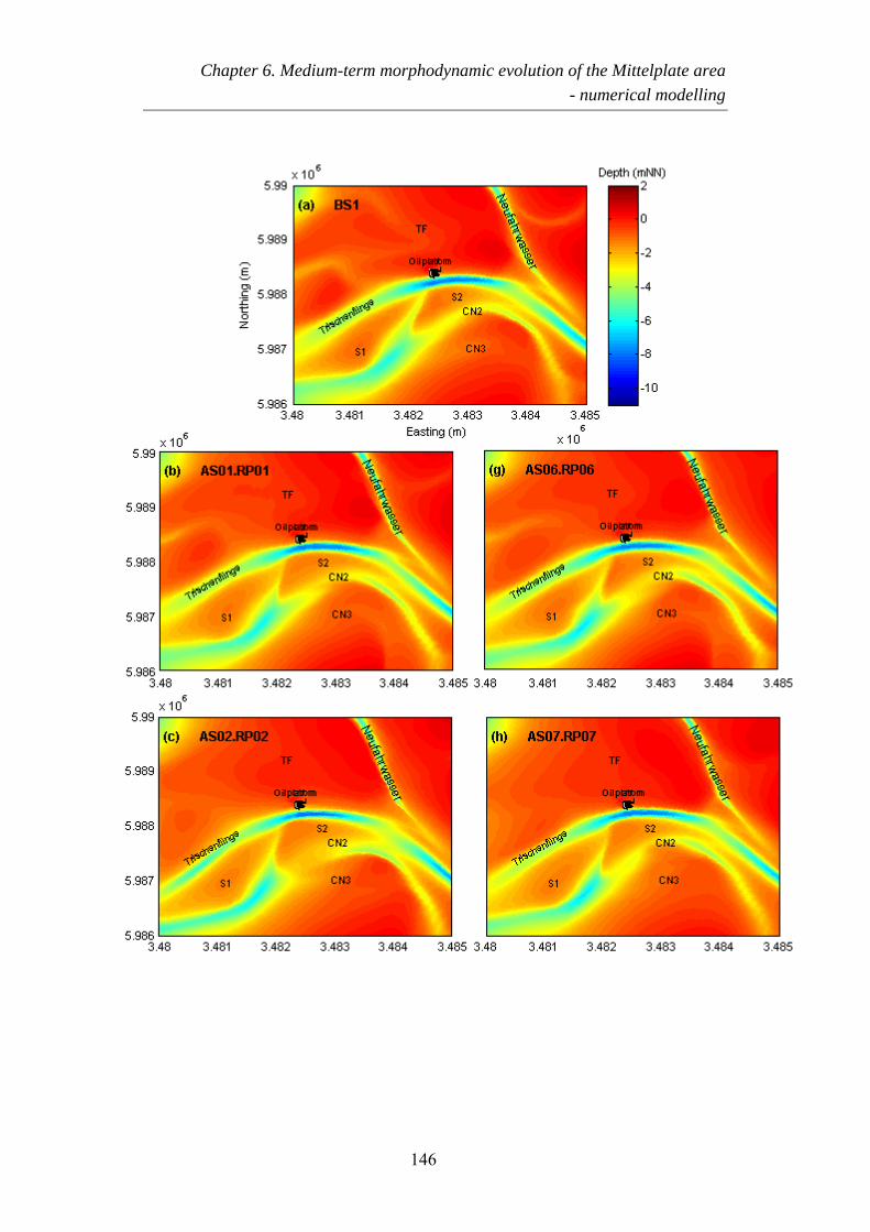
Chapter 6. Medium-term morphodynamic evolution of the Mittelplate area - numerical modelling
146
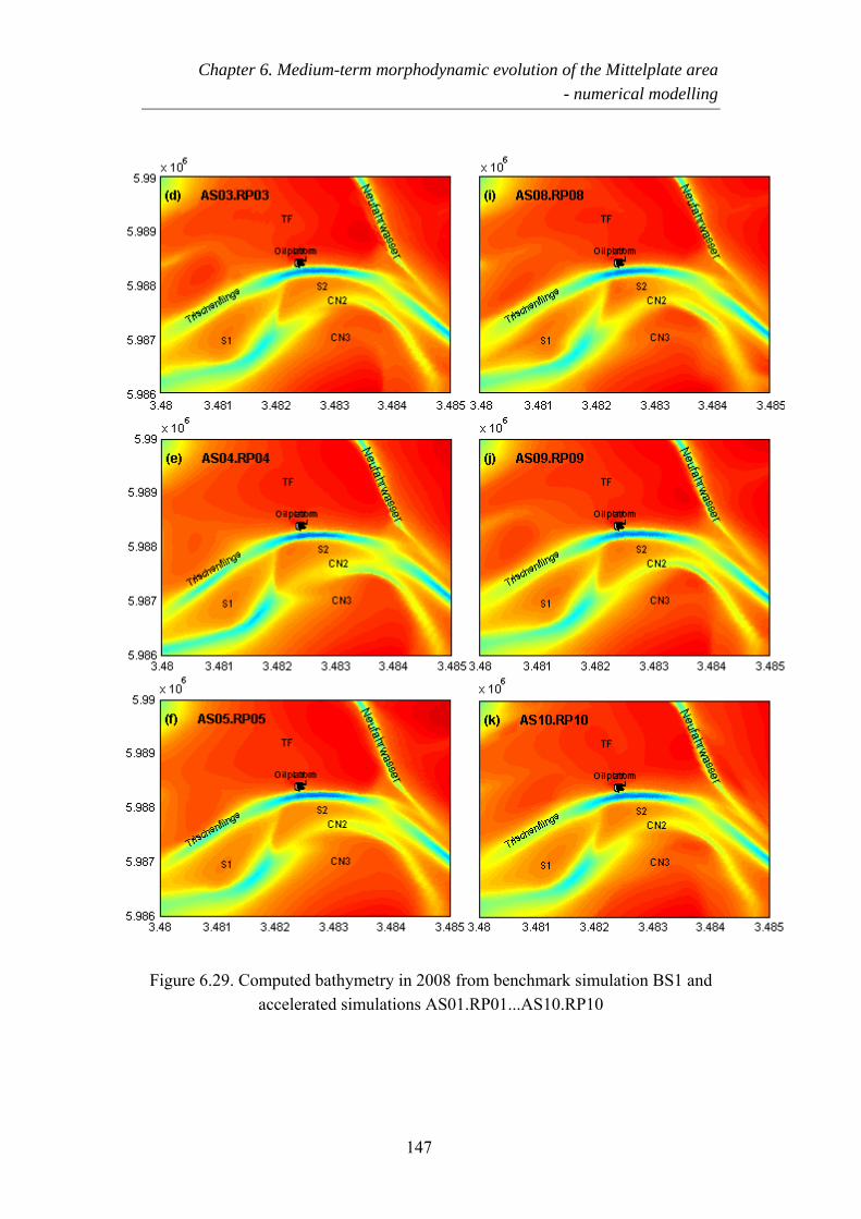
Chapter 6. Medium-term morphodynamic evolution of the Mittelplate area - numerical modelling
Figure 6.29. Computed bathymetry in 2008 from benchmark simulation BS1 and
accelerated simulations AS01.RP01...AS10.RP10
147
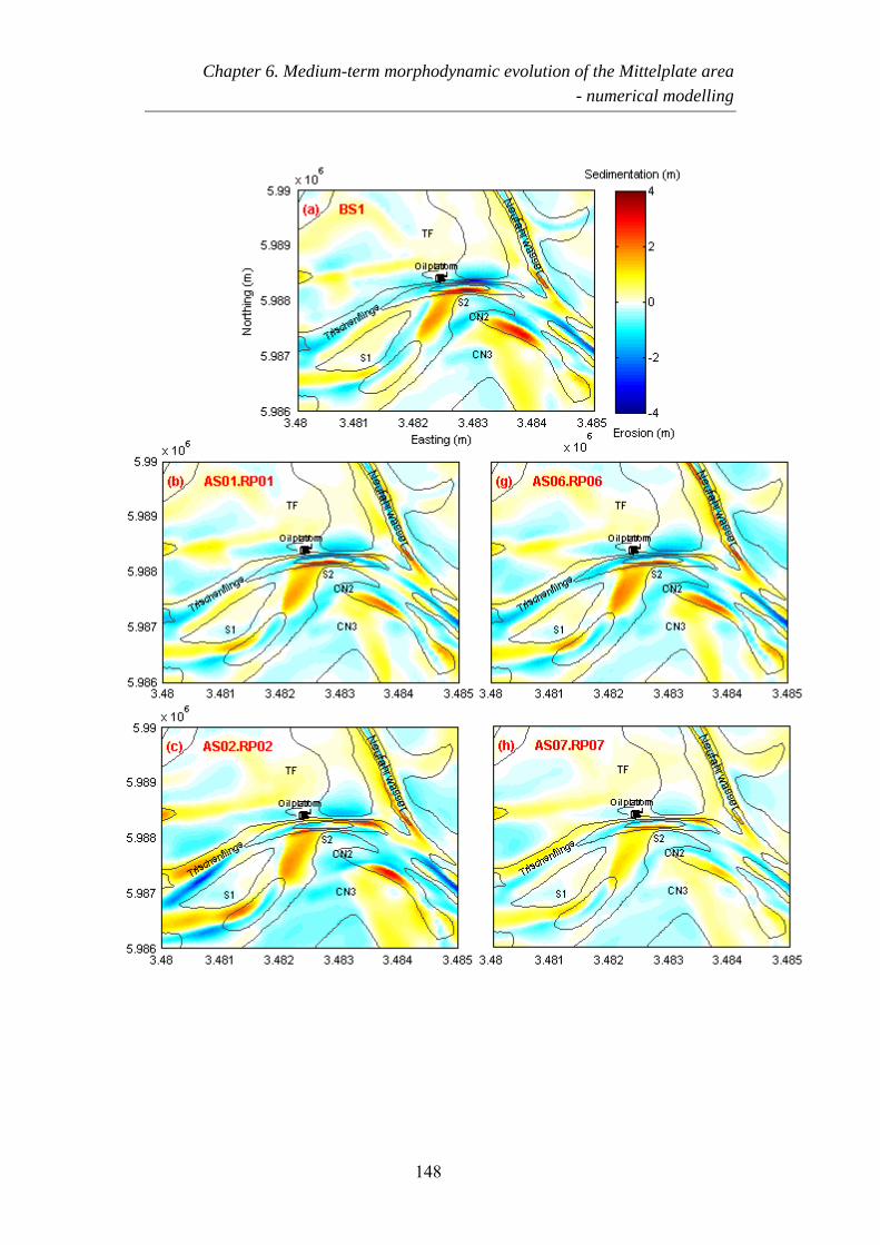
Chapter 6. Medium-term morphodynamic evolution of the Mittelplate area - numerical modelling
148
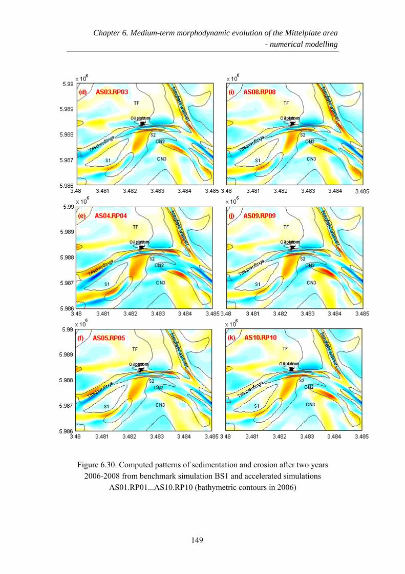
Chapter 6. Medium-term morphodynamic evolution of the Mittelplate area - numerical modelling
Figure 6.30. Computed patterns of sedimentation and erosion after two years 2006-2008 from benchmark simulation BS1 and accelerated simulations
AS01.RP01...AS10.RP10 (bathymetric contours in 2006)
149
Chapter 6. Medium-term morphodynamic evolution of the Mittelplate area - numerical modelling
6.4.7.2 Comparison of cross-section development
Comparison of the computed cross-section P2 after two years from benchmark run and 10 accelerated simulations is shown in Figure 6.31. At this cross-section, all of accelerated runs show deepening of the main channel, northward movement of the southern bank, and formation of the channel CN2, which are in the same trend with the benchmark result. Again, the slowest movement of the southern bank is observed for runs AS02.RP02, AS04.RP04, and AS05.RP05. The upper part of the northern bank computed from these runs and run AS07.RP07 shifts southward, while northward directed movement is observed for other accelerated and benchmark runs.
The resulting BSS for the 10 accelerated runs AS01.R01... AS10.R10 against the benchmark simulation BS1 is computed for the four selected cross-sections as shown in Figure 6.32. On average, RP01 and RP06 produce excellent model performance, while three RPs (RP02, RP04, and RP05) produce poor results, and the other five give good model qualification.
150
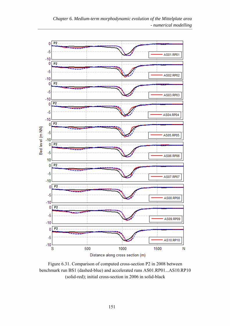
Chapter 6. Medium-term morphodynamic evolution of the Mittelplate area - numerical modelling
Figure 6.31. Comparison of computed cross-section P2 in 2008 between
benchmark run BS1 (dashed-blue) and accelerated runs AS01.RP01...AS10.RP10 (solid-red); initial cross-section in 2006 in solid-black
151
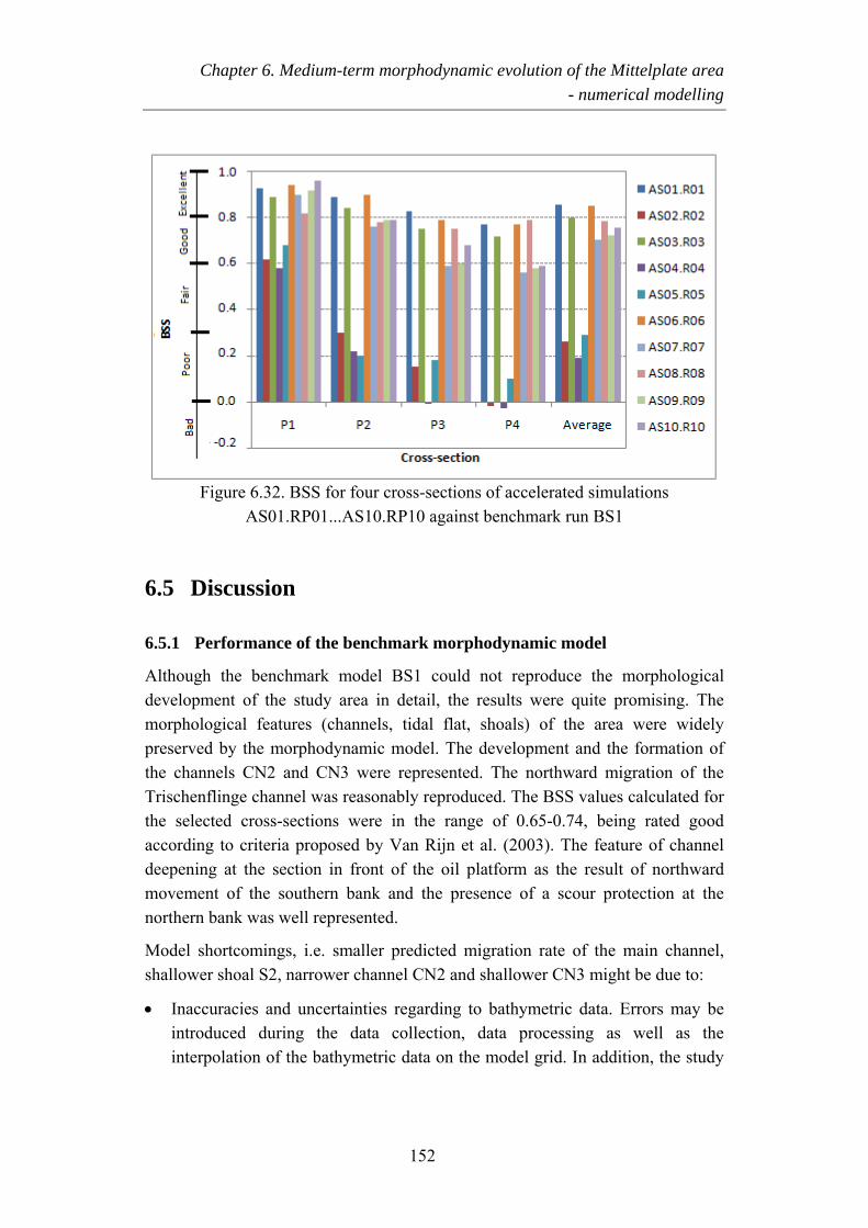
Chapter 6. Medium-term morphodynamic evolution of the Mittelplate area - numerical modelling
Figure 6.32. BSS for four cross-sections of accelerated simulations
AS01.RP01...AS10.RP10 against benchmark run BS1
6.5 Discussion
6.5.1 Performance of the benchmark morphodynamic model
Although the benchmark model BS1 could not reproduce the morphological development of the study area in detail, the results were quite promising. The morphological features (channels, tidal flat, shoals) of the area were widely preserved by the morphodynamic model. The development and the formation of the channels CN2 and CN3 were represented. The northward migration of the Trischenflinge channel was reasonably reproduced. The BSS values calculated for the selected cross-sections were in the range of 0.65-0.74, being rated good according to criteria proposed by Van Rijn et al. (2003). The feature of channel deepening at the section in front of the oil platform as the result of northward movement of the southern bank and the presence of a scour protection at the northern bank was well represented.
Model shortcomings, i.e. smaller predicted migration rate of the main channel, shallower shoal S2, narrower channel CN2 and shallower CN3 might be due to:
• Inaccuracies and uncertainties regarding to bathymetric data. Errors may be introduced during the data collection, data processing as well as the interpolation of the bathymetric data on the model grid. In addition, the study
152
Chapter 6. Medium-term morphodynamic evolution of the Mittelplate area - numerical modelling
area and surroundings were not measured completely at the same time. Therefore, data measured from different years had to be used to construct the initial bathymetry for the whole model domain.
• Lack of data on sediment composition and property. Due to the shortage of data on the horizontal and vertical composition of sediment for the entire model area, the sediment transport and morphodynamic models were constructed using only two sediment fractions with uniform grain size. In addition, for the reason of unavailability of erodibility parameters of the mud fraction, the values were chosen from published literature. Data found are of wide range and the chosen parameters were applied uniformly over the entire model domain. Sediment stratification of the bed, which might influence the erosion processes, could not be specified in the model. Although the sediment transport model was calibrated and validated against suspended sediment concentration measured along several transects within the study area, uncertainties still exist as discussed in Section 5.6. These raise the need to get more measurements of sediment properties and sediment erodibility.
• Application of depth-averaged model. Secondary flow (spiral motion) is considered as important agent for the bed level changes of river, meandering channels. In a 3D model, it is resolved directly on the vertical grid. Using 2DH version of Delft3D, the secondary flow has to be determined in an approximate way assuming that its vertical distribution is a universal function of the vertical co-ordinate. The application of 3D approach fully accounting for curvature-induced secondary flow is worth investigating.
• Limitation of the applied modelling system. Numerical models employ empirical sediment transport formulae, which do not represent all range of related conditions and processes. According to Soulsby (1997) the degree of accuracy of those formulae in the sea is not high. Much effort, therefore, has still been devoting to the improvement and the development of more suitable transport formulae (e.g. Bhattacharya et al., 2007; Camenen and Larson, 2008; Van der A et al., 2013). In addition, bank erosion is considered as an important factor for the channel migration but its related processes (e.g. avalanching mechanism) are still insufficiently understood and formulated in common numerical models (Chu et al., 2013). It is worth putting more effort on the utilization of different transport formulae and models.
• Missing of external force. During the considered two-year period, additional scour protection measures, which were not accounted for in the current
153
Chapter 6. Medium-term morphodynamic evolution of the Mittelplate area - numerical modelling
simulations, were carried out at the oil platform. These measures might influence the flow and sedimentation-erosion patterns, especially in the vicinity of the oil platform.
6.5.2 Driving forces and mechanisms of channel migration
Through the comparison of the results of the three benchmark simulations over the two-year period 2006-2008, it became obvious that the driving forces tide, wind, and waves contribute to the morphodynamic evolution in the study area in different ways within the current model setup.
The tide has proven to be the essential driving force for deepening and migrating the Trischenflinge tidal channel, for deepening the secondary channel CN2, for initiating the channel CN3, and for expanding the shoal S2. Within this context, Wilkens (2004) also found for Piep channel system located 12 km south of the study area that tide is mainly responsible for initiating, deepening, and maintaining the channels.
The migration of the Trischenflinge channel might be associated with the tidal asymmetry based on analyses of measured and modelled current velocities along the cross-sections C1, C2s, and C2l in the Trischenflinge (Section 5.2). It should be mentioned that the measuring campaigns for the investigation of the current velocity in the channels were widely conducted during calm to moderate weather conditions because the operation of the measuring vessel have to be restricted to these conditions. Therefore, the measured currents were widely driven by tide. The same pattern of ebb dominance of current velocity is obvious for the Trischenflinge channel at the three cross-sections. Through the channel route, less sediment is imported from the North Sea side than exported within a tidal cycle. The gradients of sediment transport rate result in seabed erosion of the main channel. In contrast, the connected shallow channel located between shoals S1 and S2 shows flood dominance (see Figure 5.20 for the current velocity of cross-section C2l at the southern part) and more material is transported into the channel. The sediment masses filling the channel exceed the eroded volumes so that net depositions finally prevail. Sediment transport is directed to north to the Trischenflinge channel sections and causes deposition close to and east of the oil platform. The sediments supplying the sand shoal S2 might be transported from the southern area causing the sedimentation and expansion of the shoal. These sediment supplies to the Trischenflinge may be more substantial than the amount reduced by ebb currents. It results in sedimentation along the southern bank. In
154
Chapter 6. Medium-term morphodynamic evolution of the Mittelplate area - numerical modelling
addition, the cohesive channel bed hinders the continuous deepening so that lateral migration of the channel towards north is observed.
Beside the astronomical tides, wind also influences the sediment transport. According to the modelled results, the wind was found to be a factor enhancing the migration of the main channel. In addition, it reduces erosion in the west section of the Trischenflinge and enhances deepening of the channels CN2 and CN3.
In the study area the prevailing wind direction is west with emphasis on the southwestern direction (Figure 6.3). Western wind cumbers the ebb flow and supports flood flow towards east. This may be a reason for the observation that erosion at the west section of the Trischenflinge is reduced. On the other hand, southwestern winds may favour sediment transport from south western tidal flats towards the Trischenflinge and to the shoal S2. This sediment dynamics essentially driven by southwestern wind may be one of the most important reasons for the narrowing of the Trischenflinge channel and consequently for the migration of the channel to north as its cohesive bed layers widely prevent the channel from further deepening.
Due to the enhanced water depth in the channels, the effect of waves on tidal currents is small or even negligible. However, wave orbital motion and breaking are of major importance for sediment dynamics in the shallow tidal flats. Waves may stir up sediment and induce wave driven currents which may transport sediments via bed load and suspended load to the deeper channels (Etri, 2007; Wilkens, 2004).
6.5.3 Performance of the accelerated morphodynamic models
The applicability of the input reduction, the representative period method, and acceleration technique to the medium-term morphodynamic modelling of the study area was investigated. This was done by comparing the results of morphological changes from accelerated runs on the basis of 10 representative periods with those obtained from benchmark runs. With respect to the morphodynamic behaviour of the main morphological elements displayed in Figure 4.1 and considering case "tide alone", all 10 accelerated simulations showed morphological developments similar to the results of the benchmark simulation in the two-year period. When "wind" or "wind and waves" were included in the morphodynamic simulations, some deviations in the results between 10 accelerated simulations were observed. Seven out of ten RPs
155
Chapter 6. Medium-term morphodynamic evolution of the Mittelplate area - numerical modelling
produced similar pattern of morphological development of the area, and the results resembled quite well with those from benchmark simulation. Three RPs produced some differences in the results from benchmark simulation.
These trends were also observed for the four selected cross-sections. When only "tide" was considered, the BSS values of all accelerated runs against benchmark run were close to 1, being rated as excellent. When "wind" or "wind and waves" were included, seven accelerated runs produced good and excellent performance. Three runs with RP02, RP04, and RP05 produced fair qualification when wind was included. Taking into account the effect of waves, the model using those three RPs dropped to poor performance.
It has to be pointed out that the applied approach for the input reduction is an approximation. Three hypothesised reasons for the uncertainty in the morphodynamic prediction with the application of the input reduction method in cases of inclusion of wind shall be addressed and discussed: (1) the representative periods are chosen on the base of long-term wind data instead of two-year wind data used for bench mark simulation; (2) wind classes from long-term data are not preserved in the one-month wind data; and (3) interaction between tide and wind, waves is not taken into account in approach of Boon et al. (2002).
Hypothesised reason 1. Representative periods are chosen basing on the long-term wind data
The representative periods have been selected basing on wind data in the long-term (RP_lt) instead of the data in the study two-year period (RP_2yrs). To test the hypothesis 1, the same procedure was performed following the concept of Boon et al. (2002) method to choose 10 one-month representative periods in long-term which the wind data are resemble with two-year wind data. The wind roses for these 10 representative periods are presented in Figure 6.33. It is clearly that four pairs of RP (RP04_2yrs and RP05_lt; RP06_2yrs and RP02_lt; RP08_2yrs and RP03_lt; RP09_2yrs and RP04_lt) give almost the same wind roses (see also Figure 6.6). The calculated starting time of those 2 one-month RPs is close each other. Other RPs_lt are within the first 20 RPs_2yrs. This can be explained by the resemblance of the wind fields between the two years and long-term as discussed in Section 6.3.1. It means that the use of long-term wind data instead of two-year wind data for calculating RPs used for two-year simulations is acceptable in this case.
156
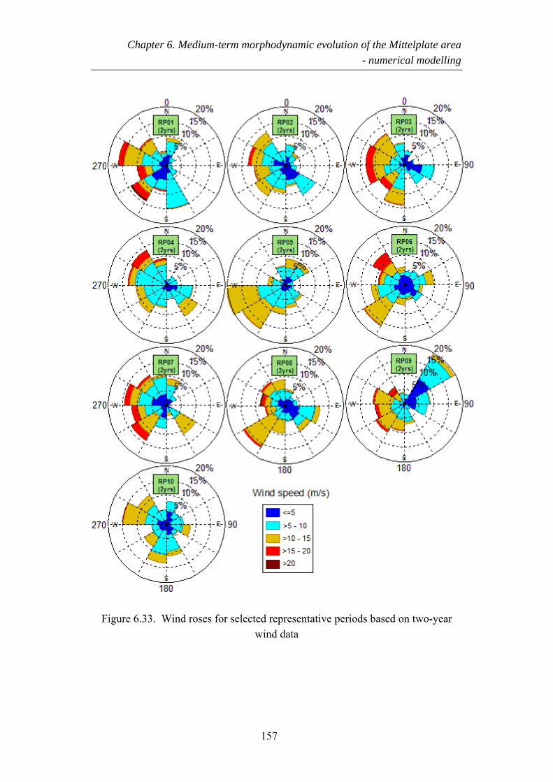
Chapter 6. Medium-term morphodynamic evolution of the Mittelplate area - numerical modelling
Figure 6.33. Wind roses for selected representative periods based on two-year wind data
157
Chapter 6. Medium-term morphodynamic evolution of the Mittelplate area - numerical modelling
Hypothesised reason 2. Changes of wind classes in the chosen RPs compared to long-term data
The approach of Boon et al. (2002) bases on averaging wind conditions a) in long-term and b) within a selected period. As the result, associated classes of wind speed and wind direction from long-term are not always preserved in the selected representative period. This is of major importance for tidal flats and channels, which are subjected to large variation of wind conditions. The changes of wind speeds and directions lead to changes of surge, wave activity, and wave induced currents
Among the other agents, the role of surge in the sediment transport and morphological changes is reported in a number of studies. Toro et al. (2005) stated that since the wind induced water level set-up is inversely proportional to the local water depth, the tidal flat areas are strongly affected by storm surges. Ridderinkhof et al. (2000) found that variations in suspended sediment concentration in the Ems-Dollard estuary are influenced significantly by variations in the water elevation (set-up/set-down) by varying wind directions.
Figures 6.34 presents the surges computed at a location in the middle of the western boundary of the model for the two-year period 2006-2008. The surge affects water level strongly, causing a maximum set-up of 1.6 m and maximum set-down of 0.5 m during the two years. A statistical analysis was performed to correlate surge to wind speed and wind direction for the period 2006-2008. The two-year wind data were categorized in 12 classes of wind direction and 5 classes of wind speed. The surges caused by each class of wind speed and direction were grouped and averaged. The average values of surge heights causing by all wind classes are illustrated in Figure 6.35. The surge is quite correlated to the wind speed and wind direction. Higher wind speed produces higher set-up or set-down for all wind directions. Onshore directed wind causes a raise in water level with the highest set-up due to the wind sector 210°-270°N, while offshore directed wind causes a set-down with the extremely low water levels due to wind sector 60°-120°N.
158
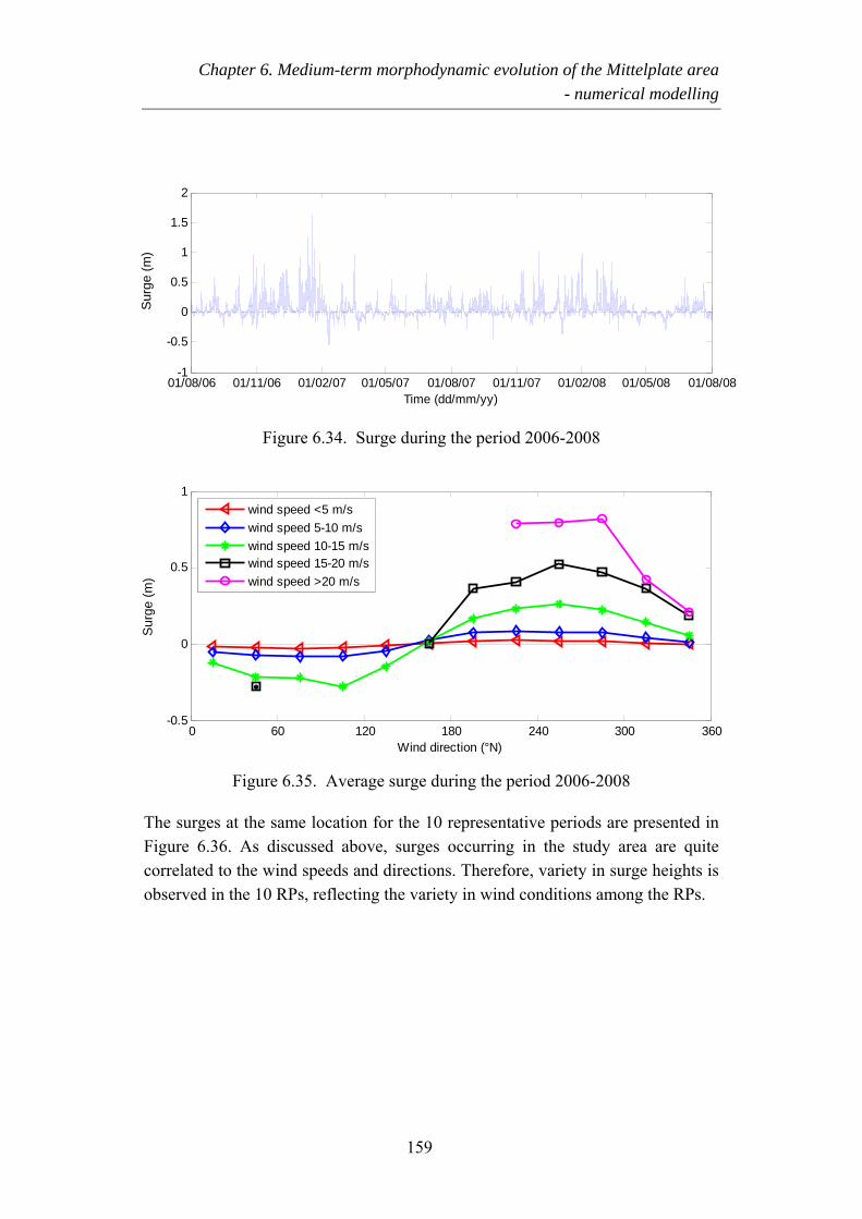
Chapter 6. Medium-term morphodynamic evolution of the Mittelplate area - numerical modelling
01/08/06 01/11/06 01/02/07 01/05/07 01/08/07 01/11/07 01/02/08 01/05/08 01/08/08-1
-0.5
0
0.5
1
1.5
2
Surge(m)
S
urge
(m)
Time (dd/mm/yy)
Figure 6.34. Surge during the period 2006-2008
0 60 120 180 240 300 360-0.5
0
0.5
1
Wind direction (°N)
Surge(m)
wind speed <5 m/swind speed 5-10 m/swind speed 10-15 m/swind speed 15-20 m/swind speed >20 m/s
S
urge
(m)
Figure 6.35. Average surge during the period 2006-2008
The surges at the same location for the 10 representative periods are presented in Figure 6.36. As discussed above, surges occurring in the study area are quite correlated to the wind speeds and directions. Therefore, variety in surge heights is observed in the 10 RPs, reflecting the variety in wind conditions among the RPs.
159
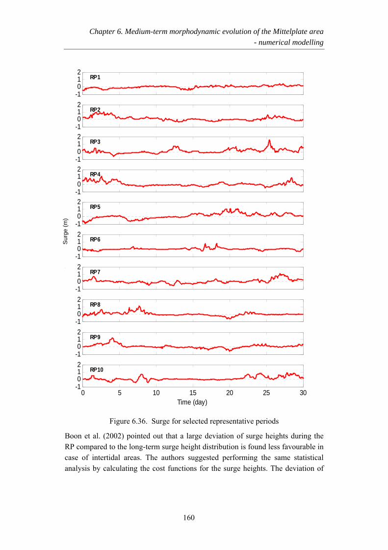
Chapter 6. Medium-term morphodynamic evolution of the Mittelplate area - numerical modelling
-1012
RP1
-1012
RP2
-1012
RP3
-1012
RP4
-1012
RP5
-1012
RP6
Sur
(gem)
Sur
ge (m
)
-1012
RP7
-1012
RP8
-1012
RP9
0 5 10 15 20 25 30-1012
RP10
Time (day)
Figure 6.36. Surge for selected representative periods
Boon et al. (2002) pointed out that a large deviation of surge heights during the RP compared to the long-term surge height distribution is found less favourable in case of intertidal areas. The authors suggested performing the same statistical analysis by calculating the cost functions for the surge heights. The deviation of
160
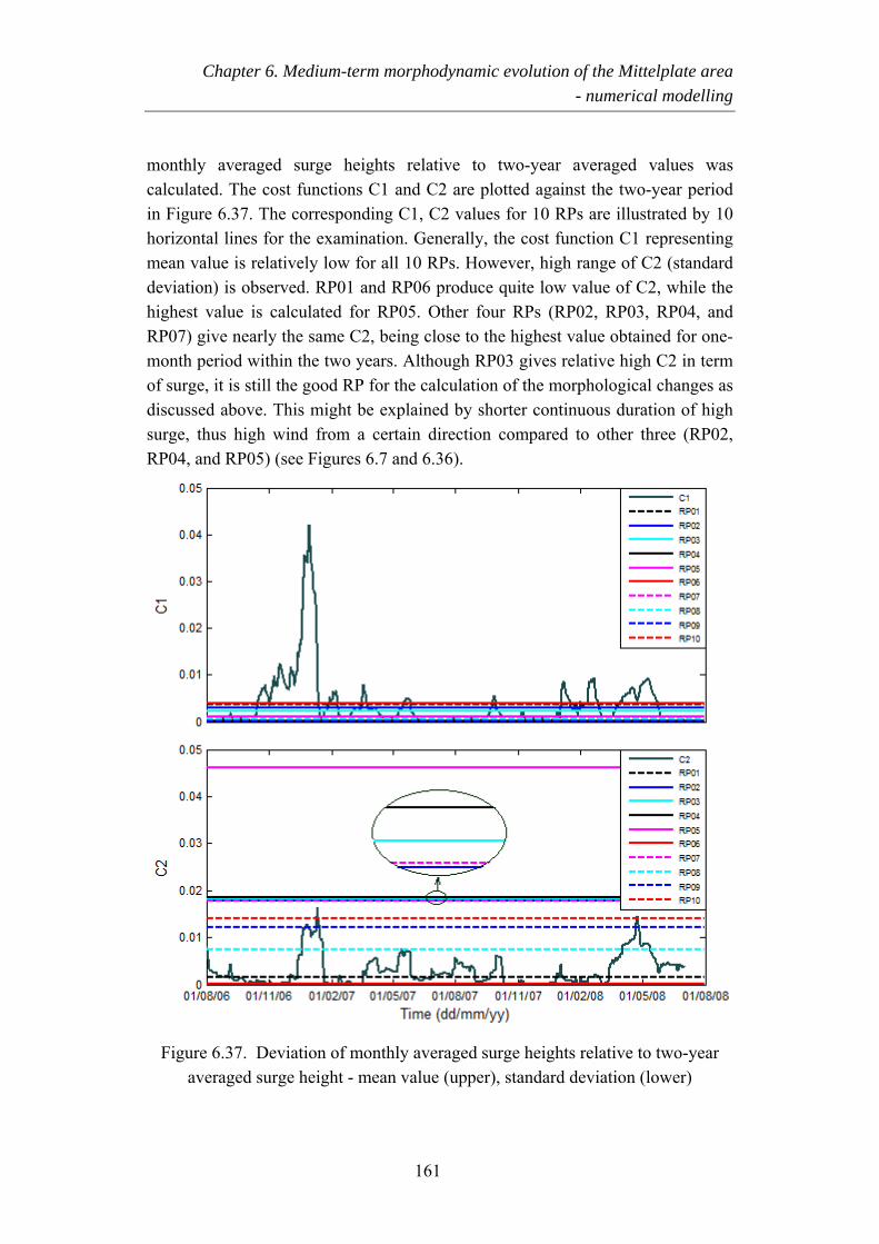
Chapter 6. Medium-term morphodynamic evolution of the Mittelplate area - numerical modelling
monthly averaged surge heights relative to two-year averaged values was calculated. The cost functions C1 and C2 are plotted against the two-year period in Figure 6.37. The corresponding C1, C2 values for 10 RPs are illustrated by 10 horizontal lines for the examination. Generally, the cost function C1 representing mean value is relatively low for all 10 RPs. However, high range of C2 (standard deviation) is observed. RP01 and RP06 produce quite low value of C2, while the highest value is calculated for RP05. Other four RPs (RP02, RP03, RP04, and RP07) give nearly the same C2, being close to the highest value obtained for one-month period within the two years. Although RP03 gives relative high C2 in term of surge, it is still the good RP for the calculation of the morphological changes as discussed above. This might be explained by shorter continuous duration of high surge, thus high wind from a certain direction compared to other three (RP02, RP04, and RP05) (see Figures 6.7 and 6.36).
Figure 6.37. Deviation of monthly averaged surge heights relative to two-year averaged surge height - mean value (upper), standard deviation (lower)
161
Chapter 6. Medium-term morphodynamic evolution of the Mittelplate area - numerical modelling
Close examination the Figure 6.7 shows a continuous duration of relatively high wind from one direction (northwest in this investigation) appearing in those three RPs. It occurred from day 2 to day 4 of RP02 with most of time the wind stronger than 12 m/s. For RP04, high wind also appeared at the beginning of the period (day 1 to day 6) with high proportion of wind in the range of 10-20 m/s. From day 16 till day 21 of RP05, the wind almost blew from the northwest direction (270°-360°N) with high wind at the second haft of this duration. This long-lasting, strong wind would cause high surge over relative long duration, strongly influence wind-induced currents and wave condition. Consequently, large morphological changes occur. On the discussion of the limitations and strengths of the morphological factor approach, Ranasinghe (2011) stated that multiplication of morphological changes that occur during storms by even a moderate fMOR may result in an unrealistic positive feedback mechanism, which will lead to erroneous results. In the case of this study, RPs containing those high wind conditions also produce poorer morphological prediction results compared to other.
The uncertainty of model prediction could be partly eliminated by preservation of the long-term data wind classes of wind speed and wind direction when calculating RP.
Hypothesised reason 3. Interaction between tide and wind, waves in long-term has been changed in 'representative period'.
By shortening the full time series of forcing process to one-month data, the interaction between tide and wind, waves has been changed. Different combinations of tide and wind, waves will result in differences in morphological changes especially in the case of tidal flats. This is demonstrated in the modelling study of Etri (2007) for the Piep channel system. The author found that sudden increases in the westerly wind speeds in conjunction with neap tidal conditions lead to high morphological activity, while gradual changes in the wind speed combined with spring tides result in low morphological changes. Within this context, study of Albers et al. (2009) based on an analysis of measured data on a tidal flat in the mouth of Elbe estuary shows that during distinct east wind dominated condition with low water; the sediment concentration is considerable above the concentrations during normal or increased tides. Therefore, it seems to be reasonable to enhance the selection of the representative conditions by taking into account the water levels.
162
Chapter 7
Conclusions and recommendations
The central aim of this thesis was to study the medium-term morphological evolution of the channel-flat environment in the Mittelplate area, Dithmarschen Bight, on the German North Sea. To achieve this aim, recorded bathymetric data over a period of six years were thoroughly analyzed with focus on the evolution of most essential morphological elements as well as of the depth contours and cross-sections of tidal channels. The morphodynamic behaviour of this area has been studied in detail on the base of process-based numerical modelling. The individual process models for simulating flow, waves, and sediment transport were set-up, calibrated, and validated against extensive data from in situ field measurements. The morphodynamic model was set-up based on the well calibrated and validated process models. The roles of different processes driving the morphodynamics and evolution of the tidal channel-flat system were investigated. The influence of an applied input reduction technique and its applicability on simulating medium-term morphological evolution was included.
The followings present main conclusions of the thesis and recommendations for further research.
163
Chapter 7. Conclusions and recommendations
7.1 Conclusions
Natural morphological development in medium-term
Based on the bathymetric observation over the six-year period 2006-2012, the significant morphodynamic changes of the study area are obvious. These include the migration of the Trischenflinge tidal channel (main channel), the deepening of channel section just in front of the oil platform, the expansion and the migration of the sand shoals south of the main channel, and the formation of two secondary channels to the south of the main channel.
Over the six-year period, significantly spatial and temporal variability in morphological response of the main channel was observed. Migration rate of the two channel banks varied in time and place, reaching to over 30 m/yr in the southward direction and over 60 m/yr in the northward direction considering the level -4 mNN. The migration rates were found to increase with an increasing of the drainage area below the level -4 mNN. Analysis of the measurements also revealed that the role of the Trischenflinge as a main drainage channel was decreasing in the course of time. The formation and enlargement of two secondary channels south of the Trischenflinge were found to be the reason for this reduction. The analysis also revealed the presence of cohesive layers in the bed of the main channel. The results from the data analyses provided understanding of the morphodynamics of the system and the background for the numerical modelling of the morphodynamic processes in the area.
Ability of the developed process models in representing the physical processes and sediment dynamics
Generally, the simulated results on hydrodynamics and sediment dynamics were in good agreements with the field measurements. The resulting RMAE for computed water levels at three measured stations was about 0.1, indicating very good model performance. With regard to current velocities, the flow patterns of the four considered cross-sections were well represented. Resulted RMAE values varied from 0.19 to 0.4, which are qualified as good and fair according Van Rijn et al. (2003). Similar to the flow model, the wave model also proved to be capable in reproducing the wave heights in the area with RMAE smaller than 0.1 in both calibration and validation periods, being rated as good and excellent.
Sensitivity and calibration test of the sediment transport model revealed the sensitivity of the model to properties of mud fraction in terms of critical shear
164
Chapter 7. Conclusions and recommendations
stress for erosion, fall velocity, and erosion parameter. The effect of waves on the sediment dynamics was found to be negligible for the considered periods when calm weather was observed. Changing grain size between 140 µm and 200 µm did not have clear effect on the suspended concentration. The resulting RMAE values for the four cross-sections C3 to C6 were in the ranges of 0.35-0.57 and 0.33-0.7 in the calibration and validation, respectively. The percentage of the concentration data falling within a factor of 2 deviation were generally high for cross-sections C3 and C4 in both calibration and validation periods, accounting for 69% to 94% of the points. Lower values were obtained for narrow cross-sections C5 and C6 (40% - 55%). The percentage of data within a factor of 5 were almost 100% for cross-sections C3 and C4, whereas 77% and 71% were obtained for C5 and C6 considering all the data sets.
Ability of the developed morphodynamic model in reproducing the observed morphological changes
Comparisons of the morphological development in two-year period resulted from the full benchmark simulation and the measurements showed that the model was able to reproduce the morphodynamic behavior of the essential morphological features qualitatively well. The gradual northward migration of the Trischenflinge channel was reasonably reproduced. The feature of channel deepening at the section in front of the oil platform as the result of northward movement of the southern bank and the presence of a scour protection at the northern bank was well represented. The development and formation of the two new channels were well predicted. Quantitatively, the model was rated as fair to excellent following the qualification of Van Rijn et al. (2003) based on calculated BSS for four selected cross-sections of the main channel.
Roles of driving forces
Based on the results of the three benchmark simulations over the two-year period 2006-2008 which different forcing was included/excluded, the varying roles of tide, wind, and waves on the morphological evolution of the area were widely recognized. Within the current model setup, the tide was found to be the important driving force for deepening and migrating the Trischenflinge tidal channel, for deepening the secondary channel CN2, for initiating the channel CN3, and for the expansion of the sand shoals investigated. The mechanism for the migration of the main channel is mainly due to tidal asymmetry of flood and ebb currents, resulting to gradients of the sediment transport rates.
165
Chapter 7. Conclusions and recommendations
The wind has proven to enhance the migration of the main channel. Important terms are the wind characteristics in the region and the orientation of the tidal channels. Winds interfere with the currents and cause the reduction of erosion in the main channel. Moreover, they favour sediment transport from the southwest to the southern bank of the Trischenflinge and from the south to the shoal S2. These sediment transport processes result in the narrowing of the channel cross-section. As the cohesive basement of the channel does not deepen, the current velocities increase. These processes induce an increasing pressure to the northern bank of the channel so that erosion occurs and the channel slowly shifts to the north.
The effect of waves was found to be important to the tidal flat. They stir up sediment and induce wave driven currents, favouring the sediments transport from the shallow areas into the channel system.
Applicability of the applied input reduction method to the medium-term morphological modelling
In total, 30 accelerated simulations applying input reduction following the concept "representative period method" and "acceleration technique" were carried out for three forcing cases (tide only, tide and wind, and all forcings). The combined methods were assessed both qualitatively and quantitatively through the comparison of the results from corresponding benchmark and accelerated simulations.
In case of "tide only" the morphological results were quite similar to those achieved through the benchmark run. If "wind" or "wind and waves" was included in the simulations, seven out of ten RPs produced relatively similar patterns of morphological development, which resembled reasonably well with the result from benchmark modelling. Three RPs produced some differences in the results from benchmark simulation. These results also revealed in the BSS values of accelerated runs against benchmark run calculated for the four selected cross-sections in the Trischenflinge. In case of "tide alone", the model performance was excellent for all ten RPs according to Van Rijn et al. (2003). Simulations with the inclusion of "wind" or "wind and waves", three out of ten RPs gave worse rating compared to other seven RPs. The uncertainty may be related to the current applied method: (1) the approach used for selection of representative periods based on cost function is such that the wind classes of wind speed and direction from long-term data are not preserved; and (2) by shortening the full time series of forcing process in long-term to 'representative period' data, the interaction between tide and wind, waves has been changed.
166
Chapter 7. Conclusions and recommendations
7.2 Recommendations
Field measurements
In the study, the sediment transport model was well calibrated and validated, and good results were achieved. However, uncertainty in sediment transport prediction, and thus morphodynamics still exists due to lack of information of sediment composition, erodibility, and underground sediment layering. The performance of sediment transport and morphodynamic models will be improved with the application of spatial varying of properties of cohesive sediment and grain size of non-cohesive sediment. These raise the need of carrying more investigation and field measurements on these parameters.
Calibration and validation of the morphodynamic model
The morphodynamic model proved to be able to reproduce the morphological behavior of the study area. The model performance could be improved through calibration and validation with the use of different sediment transport formulae and variation of the sediment parameters.
Input reduction method
The application of representative period basing on wind in conjunction with acceleration technique proved to be efficient way to simulate the medium-term morphodynamic. However, uncertainty in the results still remains. The method disregards the associated wind classes of speed and direction when shortening the long-term wind data to much shorter RP data. It is questionable if the chosen RPs containing continuous long-lasting high wind blowing from certain direction, which may result in erroneous morphodynamic prediction. In addition, the interaction of tide, wind, and waves from long-term is lost in the RP, which may contribute to the model-data deviation, especially in the case of tidal flat areas. It is, therefore, recommended to consider the representative period as a calibration parameter of the morphodynamic model. The selection of RP taking in to account the long-term wind classes and water levels would help the application of the method more effectively.
Three-dimensional model
In this study the simulations were carried out in depth-averaged version so that three dimensional processes were simplified. In the study area, the main channel has a curvature shape, which is a three-dimensional feature; the secondary flow, which is well represented in three-dimensional approach, might be important for the migration of the channel. It is worthwhile performing similar simulations in three-dimensional mode in the future.
167

168
References
Albers, T., Von Lieberman, N., Falke, E., 2009. Morphodynamic processes on tidal flats in estuaries. Journal of Coast Research, SI 56, 1325-1329.
Asp, N.E., 2004. Long to short-term morphodynamics of the tidal flats in the Dithmarschen Bight, German North Sea, PhD thesis. University of Kiel, Germany.
Bernardes, M.E.C., Davidson, M.A., Dyer, K.R., George, K.J., 2006. Towards medium-term (order of months) morphodynamic modelling of the Teign estuary, UK. Ocean Dynamics 56, 186-197.
Bhattacharya, B., Price, R.K., Solomatine, D.P., 2007. Machine learning approach to modeling sediment transport. Journal of Hydraulic Engineering 133/4, 440–450.
Booij, N., R.C. Ris, L.H. Holthuijsen, 1999. A third-generation wave model for coastal regions. Part I: Model description and validation. J. Geoph. Research 104, C4, 7649-7666.
Boon J., Kerkamp H., Dardengo L., 2002. Alternative dumping sites in the Ems-Dollard estuary, WL| Delft Hydraulics Report.
Camenen, B., Larson, M., 2005. A general formula for non-cohesive bed load sediment transport. Estuarine, Coastal and Shelf Science 63, 249–260.
Camenen, B., Larson, M., 2008. A general formula for noncohesive suspended sediment transport. Journal of Coastal Research 24/3, 615–627.
Chesher, T.J., Miles, G.V., 1992. The concept of a single representative wave. In: R.A. Falconer, S.N. Chandler-Wilde and S.Q. Liu (Editors), Hydraulic and Environmental Modelling, Coastal Waters, Ashgate, Brookfield, VT, 371-380.
169
References
Chu K., Winter C., Hebbeln D., Schulz M., 2013. Improvement of morphodynamic modeling of tidal channel migration by nudging. Coastal Engineering 77, 1–13.
Cowell, P.J., Thom, B.G., 1994. Morphodynamics of coastal evolution. In Carter, R.W.G. and Woodroffe, C. D. (Eds.) Coastal Evolution: Late Quaternary Shoreline Morphodynamics. Cambridge University Press, 33–86.
Dastgheib, A., Roelvink, J.A., Wang, Z.B., 2008. Long-term process-based morphological modeling of the Marsdiep Tidal Basin. Marine Geology 256, 90-100.
Deltares, 2008a. Delft3D-FLOW. Simulation of multi-dimensional hydrodynamic flows and transport phenomena, including sediments, User Manual.
Deltares, 2008b. Delft3D-Wave Simulation of short-crested waves with SWAN, User Manual.
De Vriend, H.J., Capobianco, M., Chesher, T., De Swart, H.E., Latteux, B., Stive, M.J.F., 1993. Approaches to long term modeling of coastal morphology: a review. Coastal Engineering 21, 225-269.
Dissanayake, D.M.P.K., Wurpts, A., Miani, M., Knaack, H., Niemeyer, H.D., Roelvink, J.A., 2012. Modelling morphodynamic response of a tidal basin to an anthropogenic effect: Ley Bay, East Frisian Wadden Sea - applying tidal forcing only and different sediment fractions. Coastal Engineering 67, 14-28.
Dittmer, E., 1938. Schichtenaufbau und Entwicklungsgeschichte des dithmarscher Alluviums, Westküste, No. 1 (2), 105-150, in German.
Erikson, L. H., Wright S. A., Elias E., Hanes D. M., Schoellhamer D. H., Largier J., 2013. The use of modeling and suspended sediment concentration measurements for quantifying net suspended sediment transport through a large tidally dominated inlet. Marine Geology 345, 96–112.
Etri, T., 2007. Effects of storms on short and medium-term morphodynamics of a tide-dominated coastal region. PhD thesis, University of Kiel, Kiel, Germany.
Gerritsen H., Vos R. J., Van der Kaaij T., Lane A., Boon J. G., 2000. Suspended sediment modelling in a shelf sea (North Sea). Coastal Engineering 41, 317–352.
Hayes, M.O., 1979. Barrier island morphology as a function of tidal and wave regime. In: Leatherman, S.P. (Eds.) Barrier Islands from the Gulf of St. Lawrence to the Gulf of Mexico.
170
References
Holthuijsen, L.H., N. Booij and T.H.C. Herbers, 1989. A prediction model for stationary, short-crested waves in shallow water with ambient currents. Coastal Engineering 13, 23-54.
Jimenez, N. (2011). An assessment of the effects of the storms on the morphological changes in the Luebeck Bay: a numerical-model-based study. Ph.D thesis, University of Kiel, Germany.
Latteux, B. (1995). Techniques for long-term morphological simulation under tidal action, Marine geology 126, 129-141.
Lesser, G.R., Roelvink, J.A., Van Kester, J.A.T.M., Stelling, G.S., 2004. Development and validation of a three-dimensional morphological model. Coastal Engineering 51, 883-915.
Luthardt, H., 1987. Analyse der Wassernahen Druck- und Windfelder über der Nordsee aus Routine-Beobachtungen, Hamburger Geophysikalische Einzelzeitschriften, A83, in German.
Mayerle, R., Razakafoniaina, T., Palacio, C., Pramono, G., 2002. Bed forms and equivalent roughness sizes in tidal channels. Proceedings of the International Conference on Fluvial Hydraulics (River Flow 2002), IAHR, Louvain-la-Neuve. Belgium.
Mayerle, R., Zielke, W., 2005. PROMORPH – Predictions of Medium‐Scale Morphodyanimcs: Project Overview and Executive Summary, Die Küste, Heft 69, 1-24.
Mehta, A.J., 1986. Characterization of cohesive sediment properties and transport processes in estuaries, In: Estuarine Cohesive Sediment Dynamics, Mehta, A.J. (Eds.), 290-325.
Muste, M., Yu K., Spasojevic M., 2004. Practical aspects of ADCP data use for quantification of mean river flow characteristics; Part I: moving-vessel measurements. Flow Measurement and Instrumentation 15, 1–16.
Nguyen D., Etri T., Runte K.H., Mayerle R., 2010. Morphodynamic modeling of the medium-term migration of a tidal channel using process-based model. Proceedings of the International Conference on Coastal Engineering (ICCE), Shanghai.
Partheniades, E., 1965. Erosion and Deposition of Cohesive Soils. ASCE Journal of Hydraulic Division 91 (HY1), 105-139.
171
References
Pejrup, M., Edelvang, K., 1996. Measurements of in situ settling velocities in the Elbe Estuary. Journal of Sea Research, 36(1/2), 109-113.
Petersen, O., Vested, H.J., Manning, A., Christie, M., Dyer K., 2002. Numerical Modelling of Mud Transport Processes in the Tamar Estuary. In: Fine Sediment Dynamics in the Marine Environment. Winterwerp, J.C. and Kranenberg C. (Eds.), Elsevier, 643-654.
Poerbandono, 2003. Sediment Transport Measurement and Modeling in the Meldorf Bight Tidal Channels, German North Sea Coast, Ph.D. Thesis. Coastal Research Laboratory, University of Kiel, Germany.
Poerbandono, R. Mayerle, 2005. Composition and Dynamics of Sediments in Tidal Channels of the German North Sea Coast, Die Küste, Heft 69, 63-92.
Ranasinghe, R., Swinkels, C., Luijendijk, A., Roelvink, J.A., Bosboom, J., Stive, M.J.F., Walstra, D.J., 2011. Morphodynamic upscaling with the MORFAC approach: dependencies and sensitivities. Coastal Engineering 58 (8), 806–811.
Reimers, H.C, 2003. Sedimentverteilung und Benthosverbreitung in den Watten der Dithmarscher Bucht als Indikator für morphodynamische Veränderungen, Abschlußbericht zum Forschungsvorhaben "Sedimorph” im GKSS Hochschulprogramm, Berichte der GKSS 18.
Ricklefs, K., Asp, N.E., 2005. Geology and Morphodynamics of a Tidal Flat Area along the German North Sea Coast, Die Küste, Heft 69, 93-128.
Ridderinkhof, H., Van der Ham., R., Van der Lee, W., 2000. Temporal variations in concentration and transport of suspended sediments in a channel-flat system in the Ems-Dollard estuary. Continental Shelf Research 20, 1479-1493.
Ris, R.C., Booij, N., Holthuisen, L.H., 1999. A third-generation wave model for coastal regions, Part II: Verification. J. Geophysical Research, 104, C4, 7667-7681.
Roelvink, J.A. (2006). Coastal morphodynamic evolution techniques. Journal of Coastal Engineering 53, 177-187.
Roelvink, D., Reniers, A., Van Dongeren, A., De Vries, J. V., McCall, R., Lescinski, J., 2009. Modelling storm impacts on beaches, dunes and barrier islands. Coastal Engineering 56, 1133–1152.
Schättler U., Doms G., Schraff C. 2009. A Description of the Nonhydrostatic Regional COSMO-Model. Part VII: User's Guide.
172
References
Simpson M.R., 2001. Discharge measurements using a broad-band acoustic Doppler current profiler, Open-File Report 01-1, US Geological Survey, Sacramento, CA.
Soulsby, R. (1997). Dynamics of marine sand: A manual for practical applications Thomas Telford Publications, London.
Steijn, R.C., 1989. Schematization of the natural conditions in multi-dimensional numerical models of coastal morphology. Delft Hydraulics. Report H526-1.
Steijn, R.C., 1992. Input filtering techniques for complex morphological models. Delft Hydraulics. Report H 824.53.
Sutherland, J., Peet, A.H., Soulsby, R.L., 2004. Evaluating the performance of morphological models. Coastal Engineering 51, 917-939.
Toro, F., Mayerle, R., Poerbandono, Wilkens, J., 2005. Patterns of hydrodynamics in a tide-dominated coastal area in the south-eastern German Bight, Die Küste, Heft 69, 25-62.
Tung, T.T., Van der Kreeke, J., Stive, M.J.F., Walstra, D.J.R, 2012. Cross-sectional stability of tidal inlets: A comparison between numerical and empirical approaches. Coastal Engineering 60, 21–29.
Van der A., D. A., Ribberink , J. S. , Van der Werf, J. J., O'Donoghue., T., Buijsrogge, R. H., Kranenburg, W. M., 2013. Practical sand transport formula for non-breaking waves and currents. Coastal Engineering 76, 26-42.
Van der Ham R., Winterwerp J.C., 2001. Turbulent exchange of fine sediments in a tidal channel in the Ems/Dollard estuary. Part II. Analysis with a 1DV numerical model. Continental Shelf Research 21, 1629–1647.
Van der Wegen, M., 2010. Modelling morphodynamic evolution in alluvial estuaries, PhD Thesis. UNESCO-IHE Institute for Water Education.
Van Rijn, L.C., 1993. Principles of Sediment Transport in Rivers, Estuaries and Coastal Seas, Aqua Publications, the Netherlands.
Van Rijn, L.C., Davies, A.G., Van de Graaff, J., Ribberink, J.S., 2001. Sediment transport modelling in marine coastal environments, Aqua Publications, Amsterdam.
Van Rijn, L.C., Walstra, D.J.R., Grasmeijer, B., Sutherland, J., Pan, S., Sierra, J.P., 2003. The predictability of cross-shore bed evolution of sandy beaches at the
173
References
time scale of storms and seasons using process-based profile models. Coastal Engineering 47, 295– 327.
Van Rijn, L.C., 2007. Unified View of Sediment Transport by Currents and Waves. II: Suspended Transport. Journal of Hydraulic Engineering, Vol. 133, No. 6, 668-689.
Verboom, G.K., De Ronde, J.G., Van Dijk, R.P., 1992. A fine grid tidal flow and storm surge model of the North Sea. Continental Shelf Research, 12(2/3), 213–233.
Villaret C., Hervouet J.M., Kopmann R., Merkel U., Davies A.G., 2011. Morphodynamic modelling using the Telemac finite element system. Computers and Geosciences 53, 105-113.
Warner J. C., Sherwood C.R., Signell R.P., Harris C.K., Arango H.G. 2008. Development of a three-dimensional, regional, coupled wave, current, and sediment-transport model. Computers & Geosciences 34, 1284–1306.
Warren, I.R., Bach, H.K., 1992. MIKE 21: a modelling system for estuaries, coastal waters and seas. Environmental Software 7 (4), 229-240.
Wilkens, J., 2004, Medium scale morphodynamics of the central Dithmarschen Bight. Ph.D thesis, University of Kiel, Germany.
Winterwerp, J.C., Van Kesteren, W.G.M., 2004. Introduction to the physics of cohesive sediment in the marine environment. Developments in sedimentology 56, Elsevier, Amsterdam.
Wright L.D., Thom B.G., 1977. Coastal depositional landforms, a morphodynamic approach. Progress in Physical Geography 1: 412–459.
Zanke, U., Mewis, P., 2002. The morphodynamic simulation system TIMOR, Wasser und Boden, 54/4, 14-22, in German.
174
Erklärung
Hiermit erkläre ich, dass die Abhandlung, abgesehen von der Beratung durch meine akademischen Lehrer, nach Inhalt und Form meine eigene Arbeit ist. Diese Arbeit hat an keiner anderen Stelle im Rahmen eines Prüfungsverfahrens vorgelegen. Außerdem erkläre ich, dass diese Arbeit unter Einhaltung der Regeln guter wissenschaftlicher Praxis der Deutschen Forschungsgemeinschaft entstanden ist und diese mein erster Promotionsversuch ist.
10. August 2015
Thi Thuy Diem Nguyen
175