Embed Size (px)
Citation preview

MATH 38071 1 Part 1
Medical Statistics
MATH 38071
Notes
(Part I)

MATH 38071 2 Part 1
Course Contents
Part I 1. Introduction - Design, Bias & Ethical Considerations
2. Basic Analyses of Continuous Outcome Measures
3. Analyses of Binary Outcome Measures
4. Sample Size and Power
5. Methods of Treatment Allocation
6. Analysis including Baseline Data.
Part II
7. Equivalence and Non-inferiority Trials
8. Analysis with Treatment Protocol Deviations
9. Crossover trials
10. Systematic Reviews & Meta-analysis
Notes, Exercises, Solutions and Past Papers with Solutions
available at
personalpages.manchester.ac.uk/staff/chris.roberts

MATH 38071 3 Part 1
Further Reading
Recommended Course Text
John N.S. Matthews An Introduction to Randomised Controlled
Trials. Taylor & Francis London (2nd
Ed. 2006 / 1st Ed. 2001)
An introductory text on clinical trials oriented towards
mathematics and statistics students. Both editions in JRL are
appropriate.
Background Reading
Books
Michael Campbell, David Machin, Stephen Walters Medical
Statistics. John Wiley London (4th Ed. 2010)
Introductory text oriented towards Medical Students. Provides
overview of topics and covers a wider range than those
considered in this course. Multiple copies available in JRL.

MATH 38071 4 Part 1
1. Introduction Design, Bias & Ethical Considerations

MATH 38071 5 Part 1
Applications of Medical Statistics
Medical research is a major field of application of statistical
methods.
Statisticians are involved with the design, conduct and analysis
of medical research projects.
Examples of medical research in which statistical methods are
applied include:
Epidemiological Studies (Determining the cause of disease
and ill health)
Clinical Trials (Evaluation of the effectiveness of treatments)
Laboratory Experimental Studies.
Development of Diagnostic Methods
Surveys of Patients and the Public
The problems raised by medical research data have led to
important developments of statistical methodology.
Statistical Methods in Medical Research
Data Analysis
Design
- Choosing the study design.
- Determining the number of subjects that need to be included.
- Developing reliable and valid measures.

MATH 38071 6 Part 1
1.1 Types of Medical Research Study
Observational Studies in Epidemiology
(i) Case control studies.
Two sample of subjects are identified (i) Cases with the disease
and (ii) Controls without. The level of exposure to the risk factor of
interest is determined for each sample.
Example Doll & Hill (1954) carried out a case-control study to
investigate whether smoking caused cancer. Patients admitted to
hospital with lung-cancer were the cases. For each case, a control
patients was selected of similar age and sex from patients admitted
to the same hospital with a diagnosis other than cancer. Past
smoking history was determined for each patient.
Table 1.1 Numbers of smokers and non-smokers among lung
cancer patients and age-matched controls
Status Non-smokers Total
Number (%) Sample
Male Lung Cancer 2 (0.3%) 649
Controls 27 (4.2%) 649
Female Lung Cancer 19 (31.7%) 60
Controls 32 (53.3%) 60
Ex 1.1 What are the limitations of this study and its design?

MATH 38071 7 Part 1
(ii) Cohort studies.
A cohort of subjects is identified and the exposure to the risk factor
measured. Subjects then followed up and outcome determined. The
outcome is compared between those who are expose and non-
exposed to the risk factor.
Example As part of the National Health and Nutrition Examination
Survey in the USA (NHANES 1) , 7188 women age 25 to 75 were
asked questions about alcohol consumption. After 10 years
subjects were traced and cases of breast cancer identified. Breast
cancer was 50% higher in drinkers than non-drinkers. The effect
was still present after adjustment for obesity, smoking and
menopausal status.
Ex 1.2 What are the limitations of this design?
Experimental studies
a) Randomised controlled trials.
b) Laboratory experiments.
Diagnostic and measurement studies
a) Testing the validity of diagnostic tests and outcome measures.
b) Testing the repeatability of a method of measurement.
c) Comparison of different measurement methods.
Systematic Reviews
a) Meta-analysis based on summary statistics.
b) Meta-analysis using individual patients data.

MATH 38071 8 Part 1
Some Terminology
Bias is a factor that tends to deviate the result of a study
systematically away from its true value.
Statistical: Related to properties of the estimator.
Experimental: Due to the design of the study.
Bias is a major concern in medical research as it may occur in
many different ways due to the complexity of clinical research.
Types of Variable in Medical Studies
Outcome Variable: This is the dependent variable of interest in a
medical study.
Exposure Variable: This could be a treatment or a risk factor for
disease and is an independent variable.
Intermediate Variable: A variable on the causal pathway from
exposure to outcome.
Exposure
Variable
Intermediate
Variable
Outcome
Variable
Confounding Variable: A variable that can cause or prevent the
outcome of interest, independently of exposure, that is also
associated with the factor under investigation.
Exposure
Variable
Confounding
Variable
Outcome
Variable
?
Confounding variables may cause bias.

MATH 38071 9 Part 1
1.2 Clinical Trials Terminology
Treatment or Intervention: therapeutic drugs, prophylactics
(preventative treatment), diagnostic tests (e.g. blood pressure),
devices (e.g. replacement hip joint), procedures (e.g. surgery) or
activities by the patient or therapist (e.g. physiotherapy).
Clinical Trial: A prospective study involving human subjects,
designed to determine the potentially beneficial effect of therapies
or preventative measures, where the investigator has control over
who receives the treatment.
Prognostic Factor: A prognostic variable is a variable that
influences outcome where the patient receives no treatment or the
current standard treatment.
Ex 1.3 Given an example of a prognostic factor in the treatment of
Cancer?
Type of Clinical Trial in Drug Development
Phase I
to establish safe/tolerable levels of a new drug often using
healthy volunteers.
Phase II
to provide evidence of potential efficacy.
to develop dosage regimes.
Phase III
to compare efficacy and effectiveness with a control therapy.

MATH 38071 10 Part 1
The Importance of a Control Group
The simplest of clinical trial is a case series evaluation in which a
group of patients who receive a new treatment are followed up and
the outcome of treatment recorded.
The problem with case series evaluations of treatments is that it is
impossible to know whether the observed outcome is
(i) the consequence of the treatment or
(ii) the natural course of the disease,
as some conditions can resolve without treatment. e.g. acute viral
infections such as the common cold.
It is important therefore to have a control treatment against which a
new treatment may be compared. In most circumstances the
control should be the current standard treatment if there is one. The
effect of a new treatment is then measured relative to the control.
Treatment Effect
In the controlled trials literature the term treatment effect means the
relative effect of one treatment on the outcome compared to
another.

MATH 38071 11 Part 1
Clinical Trials Protocol
Every well-designed clinical trial has a protocol. This documents the
purpose and procedures of the trial including:
1. The trial objectives.
2. Description of treatments being compared.
3. The study population
a. Inclusion criteria.
b. Exclusion criteria.
4. Sample size assumptions and estimate
5. Procedure for enrolment of participants.
6. Method used to allocate treatment to participants.
7. Ascertainment of outcome
a. Description and timing of assessments.
b. Data collection method.
8. Data analysis
a. Final analyses.
b. Interim analyses
9. Trial termination policy.
Published reports of clinical trial should present all this
information in detail.

MATH 38071 12 Part 1
An Early Controlled Clinical Trial - Treatment of Scurvy
(James Lind 1753 -www.jameslindlibrary.org ) “On 20 May 1747, I took 12 patients in the scurvy on board the
‘Salisbury’. The cases were as similar as I could have them. They
all … had … putrid gums, the spots and lassitude …
“They laid together … and had one diet common to all … two cider,
two others Elixir Vitril [H2SO4], two vinegar , two sea water, two
oranges and lemons , the two remaining Nutmeg.”
“One of the two receiving oranges and lemons recovered quickly
and was fit for duty after 6 days. The second was the best
recovered of the rest and assigned the role of nurse to the
remaining 10 patients.”
Ex1.4 What are the limitations of this study?

MATH 38071 13 Part 1
1.3 Bias in Controlled Trials When interpreting the results of a controlled trial one needs to
consider potential sources of bias.
SAMPLING bias - Unrepresentative nature of study sample. Patient
included may not be typical of the usual clinical population.
ALLOCATION bias – The prognosis of patients receiving each
treatment may differ.
PERFORMANCE bias - Delivery of other aspects of treatment to
each treatment group may differ e.g. In a clinical trial comparing
surgical procedures the post-operative care could differ between
treatments.
FOLLOWUP bias -Type and number of patients lost to follow-up
may differ between treatment groups.
ASSESSMENT bias – The researcher may record the outcome
more or less favourably for one treatment group than another due to
their prejudice.
STATISTICAL ANALYSIS bias – carry out multiple inferential
analyses before choosing the one most favourable to the desired
conclusion.

MATH 38071 14 Part 1
Methods for Preventing Bias
Concealment is considered to be the most effective way of
preventing bias. It refers to the practice of withholding details of the
allocated treatment from the participants in a trial (patients, care
providers, researchers or statistician).
Randomisation , that is the process of randomly choosing the
treatment a patient receives, is also important.
Bias Due to Lack of Concealment Prior to
Treatment Allocation
Knowledge of the next treatment allocation may influence
(i) Patient’s willingness to participate.
(ii) Clinician’s determination to recruit a particular patient into
trial leading to sampling and allocation bias.
These may both vary due to the characteristic or prognosis of the
patient. It is important therefore that the next treatment allocation is
concealed from both the patient and clinician prior to the decision to
join the trial being made.
After a patient has been allocated treatment it may be possible to
continue to conceal the allocation from both the patient and the
clinician.

MATH 38071 15 Part 1
Bias Due to Lack of Concealment after Treatment
Allocation
Patients
Default from treatment.
Seek alternative treatments.
Modify health related behaviour such as diet or lifestyle.
Treating health professionals
Change expectation of treatment which might affect the patient’s
response.
Influence choice of secondary treatments.
Outcome Assessor
Outcome assessor’s awareness of the patient’s treatment may
influence the measured outcome.
Knowledge of treatment may influence the patient’s self-
assessment of outcome.
Double Blind Clinical Trial Neither the patient nor the
treating/assessing clinician knows which treatment a patient is
receiving. This should reduce bias in performance of other aspects
of treatment, follow-up and assessment of outcome.
Single Blind Clinical Trial Treatment allocation is concealed from
the patient but not the clinician.
An Open / Unconcealed Clinical Trial
Patients and treating health professional both know which treatment
the patient is receiving.

MATH 38071 16 Part 1
Placebo Treatments
A placebo drug is an inactive substance designed to appear exactly
like a comparison treatment, but devoid of the active component.
A placebo should match the active treatment in appearance,
labelling and taste. The appearance of drug and placebo should
be tested before the trial to make sure patients cannot identify
the placebo.
The term placebo may also be used to describe a treatment that
has been shown to have no or minimal effect, which is to be used
as a control treatment. For example a patient information leaflet
has been shown to have no effect on outcome for some
conditions so it may be considered to be a placebo (although it
may differ in appearance from the active treatment).
Use of placebo treatment will be unethical if an established active
treatment exists that is known to be effective. In such cases an
active control group, such as best standard treatment, should be
used in place of a placebo.
Ex 1.5 Given an examples of a treatments that could/ could not be
tested in both a double blind trial.

MATH 38071 17 Part 1
Problems of Implementing Concealment
The patient may guess which of the drug treatments being
tested they are receiving from taste.
The patient, clinician or researcher may guess from appearance
or side effects.
Example: Trial of Aspirin for Myocardial Infarction Prevention
380 trial participants asked which drug they received.
50% correct, 25 % incorrect, 25% refused or selected a drug not
being tested.
Example: Staining of teeth in trials of fluoride toothpastes.
The drugs may have different dosage or frequency or delivery
systems.
Example: In the treatment of asthma different drugs may have
different frequencies. It may therefore be necessary to include
placebo drugs to give each treatment the same dosage regime.
Matching active drug and placebo may be difficult and costly.
Double-blind trials can become much more complex for chronic
diseases where the patients are on long-term medication that might
require adjustment of dosage. Procedures also need to be in place
should a patient lose their tablets. This complexity may make it
impossible for trials of some drug to be double blind.

MATH 38071 18 Part 1
1.4 The Importance of Randomisation
It enables concealment of allocation from participants prior to
randomisation thereby preventing allocation bias.
It creates treatment groups with similar distribution of patient
characteristics (both recorded and unrecorded) thereby
supporting causal inference.
It provides a logical basis for statistical inference.
Note that Randomisation is not the same as Random Sampling .
Problems of Randomisation
Lack of equipoise. May be unethical if there is already evidence
that one treatment is better or that patients may incur harm due
to one treatment.
Sampling bias. Patients that agree to participate in a randomised
trial may be atypical, for example the elderly and frail are known
to be less likely to participate.
Even with randomisation it is still possible for allocation bias to
occur due to the play of chance leading to differences in treatment
groups. This is called chance bias.

MATH 38071 19 Part 1
Summary: Biases in Controlled Clinical Trials
SAMPLING bias - Unrepresentative nature of study sample.
Solution: Modify patient recruitment – change inclusion and
exclusion criteria.
ALLOCATION bias - Prognosis of patients receiving each
treatment may differ.
Solution: Randomisation + making sure it is carried out correctly.
PERFORMANCE bias - Delivery of other aspects of treatment to
each group may differ
Solution: Concealment after randomisation, Standardisation of
additional treatments and other care procedures.
FOLLOWUP bias -Type and number of patients lost to follow-up
may differ between treatment groups.
Solution: Rigorous follow-up of all patients in both treatment groups.
ASSESSMENT or MEASUREMENT bias – The researcher may
record the outcome more or less favourably for one group.
Solutions: Conceal treatment allocation from outcome assessor.
ANALYSIS bias –Different statistical analyses may give different
results.
Solutions: Use of a predefined statistical analysis plan, Statistical
analysis carried out with the treatment allocation anonymized.

MATH 38071 20 Part 1
Figure 1.1 Schematic Diagram of a Randomised Controlled Trial
Contact potential patient requiring treatment
Check eligibility (Inclusion and Exclusion Criteria)
Randomise Randomly allocate to either New treatment or Control
New Treatment Control Treatment
Patients followed up
Statistical analysis to compare Average Outcomes for Each Treatment
Outcome measured in patients
Consent refused
Patient ineligible
Obtain informed consent
Patient agrees to enter trial

MATH 38071 21 Part 1
1.5 Ethical Issues Related to Randomised Trials
Ethical dilemmas
Is it ethical to withhold a new treatment that is thought to be
better?
Is routine practice based on inadequately tested treatments with
no proven efficacy ethical?
How much should the patient be told about the two treatments
being compared?
Ethical Principles
Patients must never be given a treatment that is known to be
inferior. Treatments should be in equipoise, that is there needs to
be uncertainty regarding which treatment is better.
Prior to recruitment patients must be fully informed about
possible adverse reactions and side-effects they may experience.
Once informed, they, or their representative in the case of non-
competent patients, must give consent, preferably in writing.
Withholding consent must not compromise the patient’s future
treatment.
Patients who have entered a trial must be able to withdraw at any
time.
Mechanism to protection the interest of the patients
Ethics committee approval of research proposals.
Individual Informed consent by the patient.
A data monitoring and ethical committee to monitor progress of
the trial.

MATH 38071 22 Part 1
1.6 Some Important Randomised Controlled Trials
Streptomycin in the treatment of pulmonary tuberculosis (UK
Medical Research Council, 1948)
- Streptomycin and bed rest vs. bed rest alone.
Important features:
- Randomisation using sealed envelopes.
- Blinded, replicated and standardised assessment of x-rays.
- Significantly better survival and radiological outcome in the
streptomycin group.
Antihistaminic drugs for the treatment of the common cold (UK
Medical Research Council, 1950) - Sample size of 1550 cases.
Important features:
- Use of a placebo to make the trial double blind.
- Important as patients asked to evaluate their own outcome.
The end result showed no difference (40% antihistamine, 39%
placebo)
Salk Polio Vaccine Trial (USA 1954)
- Observational study - school grade 2 pupils vaccinated and
compared with unvaccinated grade 1 and 3.
- Randomised controlled double blind trial – 400,000 children.
Important features:
- Large population based trial of preventative intervention.
- Demonstrated bias of non-randomised studies.
- Used a saline as a placebo vaccine.

MATH 38071 23 Part 1
2. Basic Analyses for Continuous Measures

MATH 38071 24 Part 1
2.1 Randomization and Causal Inference
One of the advantages of randomization is that it justifies causal
inference from statistical analysis rather than just association.
Consider a randomized controlled trial in which patients have been
randomized to either a new treatment (T) or a control treatment (C).
For the ith patient an outcome measure,
iY , has been determined.
A patient has two potential outcomes, say iY T and iY C . The
ideal way to estimate the effect of treatment would be to give both
treatments to each patient, and calculate the benefit of treatment as
the difference between the two potential outcomes. The treatment
effect for the ith
patient would therefore be i i iY Y CT . The
expected treatment effect is therefore,
.Pr .Pr
.Pr .Pr
.Pr .Pr
i i i
i i i i
i i
i i
E E Y Y CT
E Y Y i T E Y Y i CC i T C i CT T
E Y i T E Y i Ti T C i TT
E Y i C E Y i Ci C C i CT
In most trials a patient can only receive one treatment. If a patient
receives treatment T, the outcome iY C cannot be observed.
iY C is called a counter-factual outcome for patients that
treatment. Similarly, iY T is the counter-factual outcome for
patients receiving treatment C. Randomization allows us to assert:
i iE Y i T E Y i CC C and i iE Y i C E Y i TT T .

MATH 38071 25 Part 1
Define T iE Y i TT and C iE Y i CC .
Hence
.Pr .Pr.Pr .Pr
C CT T
T C
i T i Ci T i C
The expected values, T and
C , can be estimated by the sample
means for each group, sayTy and
Cy . Hence, the expected
treatment effect can be estimated by
ˆT Cy y .
If Y is a continuous normally distributed outcome measure, a
statistical test of the null hypothesis 0 : 0H can be carried out
using a two independent samples t-test.
In observational studies there is no randomization. Other methods
have to be used to allow one to assert that
i iE Y i C E Y i TT T and i iE Y i T E Y i CC C
Design methods
Matching of cases with controls in case-control studies.
Stratification or matching exposed and unexposed subjects in
cohort studies.
Data analysis
Using statistical modelling to adjust for confounding variables.

MATH 38071 26 Part 1
2.2 Glossary: Statistical Inference Terminology
Hypothesis test: A general term for the procedure of assessing whether “data” is consistent or otherwise with statements made about a “population”. Null Hypothesis: Represented by H0 meaning “no effect”, “no difference” or “no association” . Alternative hypothesis: Represented by H1 that usually postulates non-zero “effect”, “difference” or “association”. Significance test: A statistical procedure that when applied to a set of observations results in a p-value relative to a null hypothesis. A common misinterpretation of significant test is that failure to reject the null hypothesis justifies acceptance of the null hypothesis. p-value: Probability of obtaining a test statistic at least as extreme as the one that was actually observed, assuming that the null hypothesis is true. A common misinterpretation of a p-value is to say it is the “probability of the null hypothesis”.
Significance level () : The probability at which the null hypothesis (H0) is rejected when the null hypothesis is actually true. Typical chosen to be 5%, 1%, or 0.1%. It is also referred to as the test size. Critical value: This is the value of the test statistic corresponding to a given significance level. Confidence interval: A range of values calculated from a sample of observations that are believed with a particular probability to contain the true population parameter value. A 95% confidence interval implies that if the process was repeated again and again 95% of intervals would contain the true value in the population.

MATH 38071 27 Part 1
2.3 The Two Samples t-test
If the outcome measure Y is normally distributed, a test statistic
can be defined as ˆT C
T C
y yT
SE y y
where
ˆ .T CSE y y s , 1 1T Cn n , 2 21 1
2
T T C C
T C
Sn s n s
n n
with
Ts
and Cs being the sample standard deviations for the two treatment
groups.
A two-sided test of the null hypothesis 0 : T CH against the
alternative hypothesis 1 : T CH compares |T| with a critical value,
2 t , where is the significance level and 2T Cn n is the
degrees of freedom. If 2T t , the null hypothesis 0H is
rejected.
t/2() is the percentage point of the central t-distribution with
degrees of freedom such that upper tail probability Pr t t .
Assumptions of the two-sample t-test
(i) Subjects are independent.
(ii) The variances of the two populations being compared are equal
2 2 2
T C .
(iii) Data in each population are normally distributed.

MATH 38071 28 Part 1
One-sided and Two-sided Hypothesis Tests
A one-sided test restricts the alternative hypothesis to be either
larger, that is 1 : T CH or smaller 1 : T CH . For a two-sided
test the alternative hypothesis is 1 : T CH . A two-sided test is in
essence two one-sided tests each with significance level α/2. Based
on rejection of the null with a two-sided test one can conclude that
T C or T C .
It is recommended that two-sided tests be used unless there is a
strong a-priori reason to believe rejection in one direction is of
absolutely no interest. In medical studies this is rarely the case, so
two-sided tests are recommended and generally used. The decision
to use a one-sided test in preference to a two-sided test should be
made prior to analysing the data to prevent statistical analysis bias.
Confidence Intervals for the Difference of Means
If the outcome measure Y is normally distributed satisfying the
assumptions for the t-test , a (1-) confidence interval for the
treatment effect is given by / 2ˆ
T C T Cy y t SE y y where
ˆ 1 1T C T CSE y y s n n 2 21 1
2
T T C C
T C
n s n ss
n n
and
2T Cn n .

MATH 38071 29 Part 1
Example 2.1: Ventilation Trial. A trial of two ventilation methods
during cardiac bypass surgery. Seventeen patients undergoing
cardiac bypass surgery were randomized to one of two ventilation
schedules using 50% nitrous oxide 50% oxygen.
New For 24 hrs
Control Only during operation
The outcome measure for the trial was red cell folate level at 24 hrs
post-surgery.
Table 1.1 Red Cell Folate Level Data and Summary Statistics
Treatment Group New Control
Red Cell
Folate Level
(g/l)
251 275 291 293 332 347 354 360
206 210 226 249 255 273 285 295 309
Mean Ty 312.9 Cy 256.4
Standard deviation (s.d.) Ts 40.7
Cs 37.1
Treatment group size Tn 8 Cn 9
Figure 1.1 Dotplot of data
200
250
300
350
400
Red
Cell F
ola
te L
evels
(u
g/l)
New Treatment ControlTreatment Group

MATH 38071 30 Part 1
Ex 2.1 Calculate the point estimate of the treatment effect of the New treatment compared to the Control treatment. Point estimate of the treatment effect is
312.9ˆ 256.4 56.5T C gy y l
Ex 2.2 Using a two-sample t-test, test whether there is a significant
treatment effect using a 5% two-sided significance level.
(i) Calculate the pooled standard deviation
2 22 2
7 40.7 8 37.138.8
1 12
152
n s n sT T C C
sn nT C
(ii) Calculate the standard error of the difference between means
ˆ 11 1
38.82 18.868
19
T C T CSE y y s n n
(iii) Calculate the test statistic
312.9 256.4 56.52.995
18ˆ .86 18.86
T C
T C
y yT
SE y y
T is assumed to have a t-distribution with degrees of freedom
2T Cn n . Hence 9 8 2 15 .

MATH 38071 31 Part 1
Using Statistical Tables
A copy of the School of Mathematics Statistical Tables is available
on the module page. These give the cumulative distribution for the
t-distribution tv,q where q is the cumulative probability for q=
0.95,0.975, 0.99 and 0.995. For a two-sided test of size= 0.05, the
critical values is the value of t that give a right tail probability equal
to 0.025 (/2), which corresponds to q=1-/2=0.975 in the table.
The critical value for a two-sided 0.05 size test is therefore
t15 , 0.975=t0.025(15)=2.1314.
The null hypothesis of no treatment effect would therefore be
rejected at a 5% level, because 2.1314T . The test statistic T is
also larger than t15,0.995=t0.005(15)=2.9467. Hence, the null
hypothesis would also be rejected with a two-sided 1% significance
level. The p-value is therefore less than 0.01. Using statistical
software on can calculate the p-value for 2.995T to be 0.009.
Ex 2.3 Calculate the 95% confidence interval of the treatment effect
A (1-) confidence interval for the treatment effect is given by
/ 2ˆ
T C T Cy y t SE y y where ˆ 1 1T C T CSE y y s n n
0.02556.5 2.1314 18.86ˆT C T Cy y t SE y y
The confidence interval is therefore
Figure 2.1 STATA Output for Two-Sample t-test and CI for

MATH 38071 32 Part 1
Ventilation Trial
Two-sample t test with equal variances
------------------------------------------------------------------------------
Group | Obs Mean Std. Err. Std. Dev. [95% Conf. Interval]
---------+--------------------------------------------------------------------
Control | 9 256.4444 12.37393 37.1218 227.9101 284.9788
New | 8 312.875 14.37935 40.67094 278.8732 346.8768
---------+--------------------------------------------------------------------
diff | -56.43056 18.86238 -96.63477 -16.22634
------------------------------------------------------------------------------
diff = mean(Control) - mean(New) t = -2.9917
Ho: diff = 0 degrees of freedom = 15
Ha: diff < 0 Ha: diff != 0 Ha: diff > 0
Pr(T < t) = 0.0046 Pr(|T| > |t|) = 0.0091 Pr(T > t) = 0.9954
Ex 2.4 Briefly comment on the results of the ventilation trial.
“For patients receiving bypass surgery there was evidence that
ventilation for 24 hrs significantly increased post-operative red
folate levels by ____ gl (95% c.i. ______to ______ gl , p<______)
compared to ventilations restricted to the duration of the operation.”

MATH 38071 33 Part 1
2.4 Assumptions of the two sample t-test and
confidence interval
The two-sample t-test makes three assumptions:
I. Subjects are independent.
Independence relates to the design - are patients’ outcomes
independent or could patients be interacting in some way? In most
but not all trials this is plausible.
II. The variance of the two populations being compared are
equal 2 2 2
T C .
It is sometimes suggested that one should carry out a test
comparing variances 2 2
0 : T CH , such as Levene's test for
equality of variances, to choose between using the t-test or tests
such as the Satterthwaite or Welch test that do not assume 2 2
T C .
Unfortunately, this procedure has problems. First, the adverse
effect of unequal variance on the results of a t-test is greatest when
sample size is small, but in this circumstance the Levene’s test will
have low power to reject 2 2
0 : T CH . Secondly, this is a misuse of
statistical test, as one cannot use a test to establish the null
hypothesis 2 2
0 : T CH only the alternative 2 2
1 : T CH .

MATH 38071 34 Part 1
III. Data in each population are normally distributed.
Sometimes tests of normality, such as the Kolmogorov-Smirnov
test, are suggested to check the distributional assumptions. These
have the same problem as the Levene’s test as the assumptions of
normality is most critical where sample size is small. A better
alternative is to check the distributional assumption graphically.
Alternatively one might consider external evidence from other
studies using the same measure in similar subjects perhaps with a
much larger sample size.
Where equality of variance is not plausible the Satterthwaite test
or the Welch test can be used in place of a two-sample t-test.
Where data are non-normal data can be transformed to be closer to
normally distributed, by taking the log, square-root, or reciprocal of
the measure so that a t-test can be used. Note that inference now
relates to the transformed values. For example if a log
transformation is used inference now relates to the ratio of
geometric means. Alternatively a non-parametric methods that
make no distributional assumptions can be used such as the
Fisher-Pitman permutation test or the Mann Whitney U-test can be
used.
To simplify calculations equality of variance and normality can
be assumed in all exercises and exam questions. It is important
therefore only to be aware of the assumptions and the alternatives.

MATH 38071 35 Part 1
3. Analyses of Binary Outcome Measures

MATH 38071 36 Part 1
3.1 Treatment Effect for Binary Outcome
Measures
Suppose the outcome measure Yi is binary, examples of which
might include death, survival, recurrence or remission from disease,
sometimes referred to by the neutral term “event”. One summary of
outcome is the proportion of patients that had the event in each
treatment group, which estimates the probability of events in each
treatment, say T and C , or population rates. An alternative
parameter is the odds of the event, which is the probability of the
event divided by the probability of the complimentary event.
Table 3.1 Notation for a Trial with a Binary Outcome
Frequency Dist. Treatment Control
Yes rT rC
No nT - rT nC - rC
Total nT nC
Probability of Event
(Population proportion)
T C
Sample proportion T
T
T
rp
n C
C
C
rp
n
Odds of Event
Population Odds
1
T
T
1
C
C
Sample Odds T
T
T T
rq
n r
CC
C C
rq
n r

MATH 38071 37 Part 1
The effect of treatment can be measured in three ways
Rate or Risk Difference, T CRD ,
Rate Ratio, T
C
RR
Odd Ratio,
1 1
1
1
T
T T C
C T C
C
OR
3.2 Inference for the Rate Difference
The rate difference (RD) is estimated by ˆT CRD p p where
TT
T
rp
n and C
C
C
rp
n . The numbers of successes rT and rC have
distributions ,T TBin n and ,C CBin n . From properties of the
binomial distribution the variance of rT equals . 1T T Tn .
Hence the proportion TT
T
rp
n is given by
2
1T T T
T
T T
Var rVar p
n n
and similarly for CVar p .
Since treatment groups are independent, it follows that
1 1T T C C
T C T C
T C
Var RD Var p p Var p Var pn n
.
This can be estimated by substituting pT and pC for T and C .
Hence,
1 1ˆ ˆˆ T T C C
T C
T C
p p p pSE RD SE p p
n n
.

MATH 38071 38 Part 1
This is used for confidence interval construction.
Under the null hypothesis0 : 0H RD ,
T C say. The pooled
proportion can be estimated by T C T T C C
T C T C
r r n p n pp
n n n n
with
T T C C
T C
n nE p
n n
.
Hence, the null standard error can be defined as
1 1 1 1ˆ ˆ 1null
T C T C
p p p pSE RD p p
n n n n
.
This is used for statistical inference on 0 : 0H RD .

MATH 38071 39 Part 1
Two-Sample z-test of Proportions
A test of 0 : 0H RD vs
1 : 0H RD can be constructed as
ˆ
ˆˆ ˆT C
RD
null T Cnull
RD p pZ
SE p pSE RD
.
Under assumptions given below ZRD is approximates a
standardised normal distribution, 0,1N . This is the two sample z-
test for proportions corresponding to the two-sample t-test for
means.
Two-Sample z-test of Proportions
ˆT C
RD
null T C
p pZ
SE p p
and
1 1ˆ 1null T C
T C
SE p p p pn n
where T C
T C
r rp
n n
.
For an -size two-sided test of 0 : 0H RD vs 1 : 0H RD compare
RDZ against critical values defined by 2z . Alternatively, the p-
values for the two-sided test is given by 2 1 RDZ where is
the cumulative density of the standardized normal distribution.
Confidence Interval
A (1-) confidence interval for T CRD is given by
/ 2ˆ
T C T Cp p z SE p p
where 1 1ˆ T T C C
T C
T C
p p p pSE p p
n n
Assumptions
(i) subjects are independent and
(ii) nT p, nC p , nT (1-p), nC (1-p) are all greater than 5.

MATH 38071 40 Part 1
There are improved formulae for the z-test and confidence interval
that include a continuity correction to improve the normal
approximation of the binomial distribution, but these methods are
not considered any further in this module.
Example 3.1. The Propranolol Trial
91 patients admitted with myocardial infarction were randomly
allocated to propranolol or placebo. The table below records
survival status of propranolol treated patients and control patients
28 days after admission
Status 28 days after admission
Propranolol Placebo
Alive 38 29 Died 7 17
Total 45 46
Ex 3.1 For the Propranolol Trial data calculates the point estimate
of the difference in survival rate
For the Propranolol group the rate =
For the Placebo group the rate = Therefore RD= Ex 3.2 Check the assumptions of z-test of proportions
The assumptions of the z-test of proportions are that nT p, nC p , nT
(1-p), nC (1-p) are all greater than 5.
T C
T C
r rp
n n
Hence nT p, nC p , nT (1-p), nC (1-p) are

MATH 38071 41 Part 1
Ex 3.3 Compare the survival rate for the two treatments using a z-
test of proportions.
From above p=0.736. , T CT C
T C
r rp p
n n
1 1ˆ 1null T C
T C
SE p p p pn n
ˆT C
RD
null T C
p pZ
SE p p
From table of the normal distribution the critical values of a two-
sided 5% level test are
1.960
2 1p value Z
Note that it does not matter whether the z-test is compute based on
the proportion who have died or the proportion still alive.
Normal Distribution and Normal Statistical Tables
Suppose is the cumulative distribution function of a standardized
normal distribution 0,1N . In this module the percentage point z of
a random variable Z with distribution 0,1N is the value such that
1P Z z z .
Tables provided by the Mathematic department define a percentage
point the percentage point qz to be the value such that
q qZ z zP q .

MATH 38071 42 Part 1
Table 3.2 Summary of Important Percentage Points of the Standardized Normal Distribution
q z
0.2 0.8 0.8416 0.1 0.9 1.2816 0.05 0.95 1.6449
0.025 0.975 1.9600 0.01 0.99 2.3263
0.005 0.995 2.5758
Calculation of 95%-Confidence interval for difference of proportions
Ex 3.4 For the Propranolol Trial calculate a 95% confidence interval of the difference in survival rate for the two treatments.
1 1ˆ T T C C
T C
T C
p p p pSE p p
n n
From tables 0.025z
(1-) confidence interval calculated from
/ 2ˆ
T C T Cp p z SE p p
Ex 3.5 Briefly comment on the effect of propranolol treatment on
survival.
“ There was evidence that for patients admitted with myocardial
infarction those treated with propranolol had an improved survival at
28 days post admission ( ) as compared to untreated
patients ( ) with a difference of (95% c.i. to
p-value = ).”
Note. In the critical appraisal paper they write p to represent th p-
value

MATH 38071 43 Part 1
Figure 3.1 STATA Output for z-test of proportions for the
Propranolol Trial Data based on numbers of death before 28 days
Two-sample test of proportion Placebo: Number of obs = 46
Propranolol: Number of obs = 45
------------------------------------------------------------------------------
Variable | Mean Std. Err. z P>|z| [95% Conf. Interval]
-------------+----------------------------------------------------------------
Placebo | .3695652 .0711683 .2300779 .5090526
Propranolol | .1555556 .0540284 .0496619 .2614493
-------------+----------------------------------------------------------------
diff | .2140097 .0893532 .0388806 .3891387
| under Ho: .0923926 2.32 0.021
------------------------------------------------------------------------------
diff = prop(Placebo) - prop(Propranolol) z = 2.3163
Ho: diff = 0
Ha: diff < 0 Ha: diff != 0 Ha: diff > 0
Pr(Z < z) = 0.9897 Pr(|Z| < |z|) = 0.0205 Pr(Z > z) = 0.0103
Numbers Need to Treat
Numbers need to treat (NNT) is defined as the average of the
number of patients that need to be treated to prevent one additional
bad outcome. This measure is popular with doctors as it gives them
a measure of the population level benefit of any treatment.
NNT is simply the reciprocal of the rate difference RD, that
1NNT
RD .
A confidence interval of NTT can be found by taking the reciprocal
of the confidence limits of RD. Note that the confidence interval
becomes nonsensical if the confidence interval of RD includes
zero.
Ex 3.6 Calculate the point estimate and 95% confidence interval of
NNT for propranolol .
MATH 38071 44 Part 1
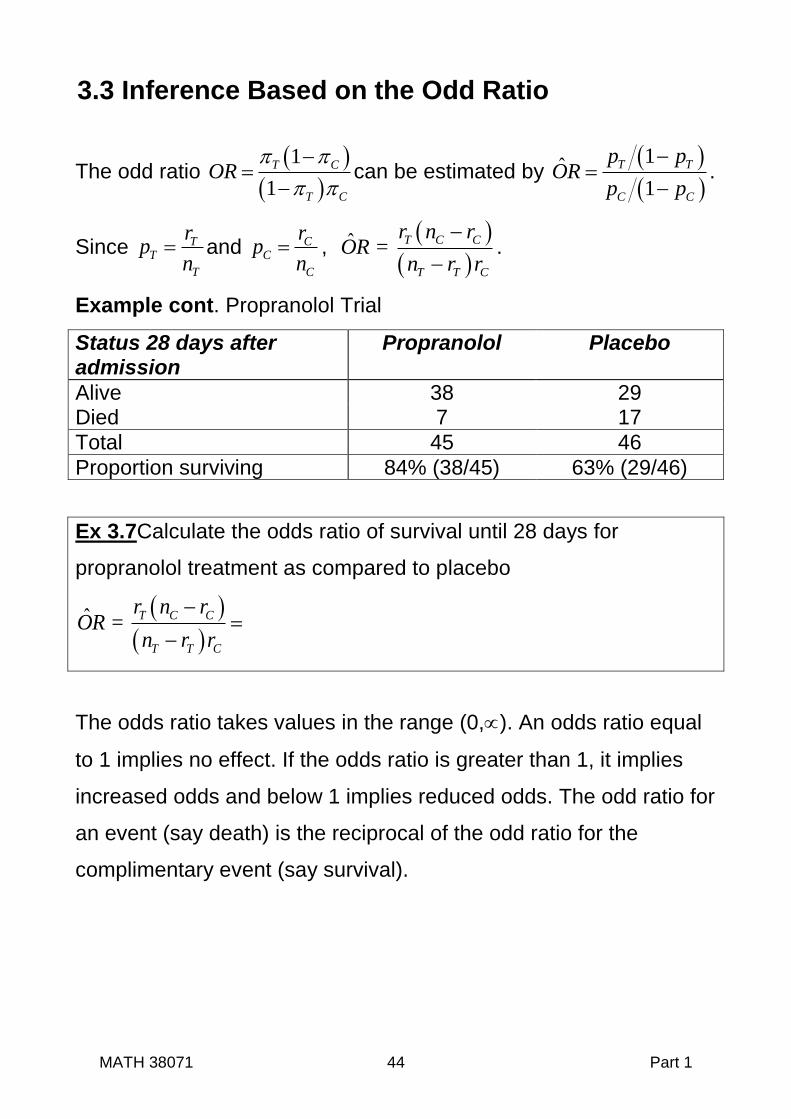
3.3 Inference Based on the Odd Ratio
The odd ratio
1
1
T C
T C
OR
can be estimated by
1ˆ1
T T
C C
p pOR
p p.
Since TT
T
rp
n and C
C
C
rp
n ,
ˆ =
T C C
T T C
r n rOR
n r r.
Example cont. Propranolol Trial
Status 28 days after admission
Propranolol Placebo
Alive 38 29 Died 7 17
Total 45 46
Proportion surviving 84% (38/45) 63% (29/46)
Ex 3.7Calculate the odds ratio of survival until 28 days for
propranolol treatment as compared to placebo
ˆ =
T C C
T T C
r n rOR
n r r
The odds ratio takes values in the range (0,). An odds ratio equal
to 1 implies no effect. If the odds ratio is greater than 1, it implies
increased odds and below 1 implies reduced odds. The odd ratio for
an event (say death) is the reciprocal of the odd ratio for the
complimentary event (say survival).

MATH 38071 45 Part 1
Confidence Intervals for Odds Ratios
The sampling distribution of odds ratio (OR) is poorly approximated
by the normal distribution. Instead, confidence intervals for the
loge OR are calculated and then exponents (anti-logs) taken to get
the confidence interval of the odds ratio. This means that the
resulting confidence interval is not symmetric about the point
estimate.
With the notation above 1 1 1 1ˆloge
T T T C C C
SE ORr n r r n r
This can be derived as follows:
1ˆlog log1
T C
e e
T C
p pVar OR Var
p p
log log
1 1
T Ce e
T C
p pVar
p p
log log1 1
T Ce e
T C
p pVar Var
p p
(*)
because treatment groups are independent. Approximate standard
errors can be calculated using the Delta Method, which is based on
a Taylor Series approximation. This states that
2
x E xVar f x f x Var x
.
Considering log1
TT e
T
pf p
p
’
.
Hence
1 1 1
1 1T
T T T T
f pp p p p

MATH 38071 46 Part 1
Since E p and 1T T
T
T
Var pn
,
it follows that
2
11 1log
1 1 1
T TTe
T T T T T T T
pVar
p n n
.
Similarly,
1
log1 1
Ce
C C C C
pVar
p n
.
Substitution in the equation (*) above give
1 1ˆlog1 1
e
T T T C C C
Var ORn n
1 1 1 1
1 1T T T T C C C Cn n n n
.
The standard error can be obtained by substitution of pT and pC for
T and C .
Hence
1 1 1 1ˆlog1 1
e
T T T T C C C C
SE ORn p n p n p n p
1 1 1 1
T T T C C Cr n r r n r
as required ■
Using this result the (1-) confidence interval of loge OR is
/ 2
1 1 1 1log T C C
e
T T C T T T C C C
r n rz
n r r r n r r n r
Confidence intervals for the odds ratio are obtained by taking the
exponents.

MATH 38071 47 Part 1
Ex 3.8 For the data from the Propranolol trial calculate the 95%
confidence interval for the odd of survival at 28 days for propranolol
as compared to placebo.
ˆloge OR
1 1 1 1ˆ ˆloge
T T T C C C
SE ORr n r r n r
95% Confidence intervals of ˆloge OR
are given by
1.96 , that is
Taking exponentials 95% Confidence interval of OR is ( , )
Hypotheses Test for the Odds Ratio
A test of the null hypothesis Ho:OR=1 could be based on the
statistic
ˆlog
ˆ ˆlog
e
lor
e
ORZ
SE OR
i.e. test 0
ˆ: log 0eH OR
. In practice
one does not do this as the test of the null Ho: OR=1 is equivalent to
the test based on the rate difference, Ho: RD=0, which is preferable
as it does not depend an approximate standard error determined
using the delta method. The p-value for the z-test of proportions
calculated above is therefore used for hypothesis tests of the odds
ratio in preference to the statistic lorZ .

MATH 38071 48 Part 1
Ex 3.9 Summarize the results of the propranolol trial based on
Odds Ratios analysis.
“ There was evidence that propranolol increased the odds of
survival compared to placebo (OR= 3.18, 95% c.i. 1.17 to 8.67,
p=0.022).”
Interpretation of the Odds Ratio
Many people find odds ratios difficult to interpret, but the odds ratio
is an important measure of effect in medical statistics. One reason
for this is that the odds ratio can be estimated by logistic regression,
which enables estimation of the odds ratio adjusted for other
variables. This is very important for observational studies as it
enables adjustment of effects for confounding variables. What is
more the odds ratio is essential for case control studies as it is not
possible to estimate either the risk difference or the risk ratio of the
outcome due to the way in which subjects have been selected.
3.4 Analyses Based on the Rate Ratio
The rate ratio T
C
RR
can be estimated by ˆ T
C
pRR
p
Confidence intervals for the rate ratio, also called the risk ratio, can
be constructed in a similar way to the odds ratio. As with the odds
ratio the hypotheses test for the rate ratio is equivalent to that for
the rate difference (RD) and so the z-test for proportions is still used
to test hypotheses.

MATH 38071 49 Part 1
4. Sample Size And Power In Parallel Group Clinical Trials

MATH 38071 50 Part 1
4.1 Sample size and power
Sample calculation is important for two reasons
If too few patients are recruited, the trial may lack statistical
power, so the study is likely to fail to answer the question it is
attempting to address.
If more patients than the minimum required to answer the
question are recruited, some patients may be exposed to an
inferior treatment unnecessarily.
As patient recruitment is often difficult, the first reason is generally
more important than the second.
Two approaches to sample size in clinical trials
(i) Predetermined trial size
The number of patients to be recruited is fixed before the trial starts.
(ii) Trial size determined by outcome
Statistical analyses, called interim analyses, are carried out
intermittently as the trial progresses. The trial is stopped if benefit or
harm is demonstrated. Whilst this type of trial design is attractive,
outcome needs to be determined shortly after recruitment so the
interim analysis can be completed. Statistical analysis is also much
more complex as it needs to account for multiple statistical testing.
Predetermine sample size is much more often used as they are
easier to organise and run. To maintain an overall significance
level of , called the family wise error rate, the test size for each

MATH 38071 51 Part 1
test is made smaller, but this is complex as sequential statistical
tests are not independent. This is a hybrid called a group sequential
trial design that has a maximum sample size but also has interim
analyses to allow early termination.
4.2 Statistical Power Consider a trial comparing a new treatment group (T) to a control
group (C). Suppose is the treatment effect. To test for a treatment
effect ( 0) the two-sided hypothesis are:
Null hypothesis H0: =0
Alternate hypothesis H1: 0
If H0 is rejected, when H0 is true, a Type I or false positive error has
occurred.
Pr [Type I error] = Pr [ Reject H0 | H0] = ,
which is the significance level.
If instead H0 not rejected, when H0 is false, a Type II or false
negative error has occurred. Define as the probability of a Type II
error. This depends on the significance level and the magnitude
of the effect that we wish to detect.
Pr [Type II error] = Pr [Not reject H0 | H1 ] = (, )
Statistical Power is the probability that a test will detect a difference
with a significance level . Power =1 - (, )

MATH 38071 52 Part 1
Calculation of Power
As previously defined the test statistic of a two sample t-test is ˆ
T
where 1 1T Cn n .
Fig 4.1 Illustration of power calculation for a normally distributed
outcome for a two-sided two-sample t-test.
(i) Smaller Sample Size – Low Power
(ii) Larger Sample Size - Increased Power

MATH 38071 53 Part 1
Under H1 the test statistic ˆ
T
has the non-central t-distribution.
If F is the cumulative distribution of the non-central t-distribution
with 2T Cn n degrees of freedom and non-centrality parameter
, then
2 21 , 1 ( 2) ( 2)T C T CPower F t n n F t n n
4.3 Sample Size Calculation for Continuous
Outcome Measures
Because the central and non-central t-distributions have degrees of
freedom determined by sample size there is not a closed form
formula for sample size based on this distribution. Instead, we shall
use the normal distribution as an approximation for the central and
non-central t-distributions to get an approximate formula.
For a normally distributed outcome variable the approximate
number of subjects required in each of two equal sized groups
to have power 1- to detect a treatment effect using a two group t-
test with an two-sided significance level is
2
2
22
2n z z
,
where is the within group standard deviation.
Assuming n is sufficiently large such that a normal approximation to
the central and non-central t-distribution is adequate, the test

MATH 38071 54 Part 1
statistic T has the standard normal distribution 0,1N under Ho and
,1N
under H1. Therefore
2 21 1Power z z
[1]
where 1 1T Cn n and is the cumulative distribution for
0,1N . The second term on the RHS of equation [1] is negligible,
therefore
21 1Power z
.
Hence
2z
.
Since z1, it follows that 2z z
giving 2z z
. [2]
If equal sized groups are assumed T Cn n n , then n2 .
Substitution into [2] gives 22
nz z
.
Rearrangement gives 2
2
22
2n z z
as required■

MATH 38071 55 Part 1
Power
From the above derivation the power of a trial with two groups of
size nT and nC to detect an treatment effect of magnitude using a
two group t-test with an two-sided significance level is
21 z
where is the cumulative distribution function of
0,1N and 1 1T Cn n .
Figure 4.2 Plot of Power (1 - ) against standardised effect define
as for various total sample sizes for a two sample t-test
assuming a 5% two-sided significance level and equal size groups.

MATH 38071 56 Part 1
Ex 4.1 A clinical trial is planned to compare cognitive behavioural
therapy (CBT) and a drug therapy for the treatment of depression.
The primary outcome measure is the HoNOS scale, which is a
measure of impairment due to psychological distress. From
published data the within group standard deviation of HoNOS is
estimated to be 5.7 units.
(i) Calculate the sample size required for each treatment to
detect a treatment effect of 2 units on the HoNOS scale
with 80% power and a two group t-test with a 0.05 two-
sided significance level.
= =
= =
z/2 = z =
Using the formula, 2 2
22
2
S
n z z
Sample size per group =
Software assuming t-distribution give sample size per group= 129
(ii) Assuming the same significance level, what power would
the study have with only 50 patients into each treatment?
2
21 1.96
5.7 1/50 1/501
1 0.58 0.42
Power z
Note Power determine using statistical software that assumes a t-distribution rather than a normal approximation equals to 0.41.

MATH 38071 57 Part 1
The Effect of Unequal Randomisation on Sample Size Suppose the allocation ratio between treatment groups is 1:k. i.e.
for every patient allocated to one group on average k are allocated
to the other. For a continuous outcome, it can be shown that the
total sample size to give the same power is increased by
2
1
4.
kN
k
where N is the sample size assuming equal allocation. Derivation
of this formula is set as an exercise.
Table 4.1 Increase in total sample size required to maintain power
when allocation is unequal
Allocation
Ratio k
Percentage Increase
in sample size
2
1
4.
k
k
3:2 1.5 4.2%
2:1 2 12.5%
3:1 3 33.3%
4:1 4 56.3%
From table 4.1 it can be seen that as the allocation ratio increases
the sample size to achieve the same power increases, but the effect
is not great until the allocation ratio exceeds 2:1.

MATH 38071 58 Part 1
Practical Considerations when Calculating Sample size
To estimate sample size we need to choose a value of . One
might take to be the minimum difference that is thought to be
clinically important, which is called the minimum clinically
important difference (MCID). Alternatively, one may have an idea
of the size of the treatment effect and choose that instead.
An estimate of is needed to complete the calculation. This is
often obtained from previous trials using the same outcome in a
similar population.
Power (1-) = 0.8 or 0.9 and a significance level of 5% are
generally used.
The above formula is for a two-side significance test. The sample
size formula for a one-sided test is obtained by replacing /2 by
in the formulae derived.
Where a trial compares several outcomes, it is usual to specify
one measure as the primary outcome measure for which
sample size is then determined.

MATH 38071 59 Part 1
4.4 Sample Size Calculation for Binary Outcome Measures For a binary outcome measure the approximate number of subjects
required in each of two equal sized groups to have power (1-) to
detect a treatment effect T C using a two sample z-test of
proportions with a two-sided significance level is
2
2
2
2 1 1 1
T T C Cz zn
were2
T C
.
Suppose Tp and Cp are the observed proportion of successes in
each group. The test statistic for the two-tailed z-test of proportions
test is 1 .
T Cp pT
p p
with 1 1T Cn n and
T C
T C
r rp
n n
.
The distribution of T is approximately 1 1
0, 1T C
Nn n
under
the null hypothesis, with critical values 2z and 2z for an
level two-sided test with T T C C
T C
n n
n n
.
Suppose T C is the effect under the alternative hypothesis.
Without loss of generality assume that > 0. The power 1 equals
2 2Pr 1 Pr 1T C T Cp p z p p z .

MATH 38071 60 Part 1
The distribution of T cp p under the alternative hypothesis is
1 1, T T C C
T C
Nn n
.
Since > 0, 2Pr 1T Cp p z will be negligible.
Therefore
2. . 1
1 1 1 1T T C C
T C
z
n n
where is the
cumulative density function of 0,1N . Since 1 z , it
follows that
2. . 1
1 1T T C C
T C
zz
n n
.
Assuming equal size groups T Cn n n , then n2 .
Rearrangement gives
2
1 1 2 1T T C Cz z
n n
Further rearrangement gives
2 2 1 1 1T T C Cz zn
so that
2
2
2
2 1 1 1T T C Cz zn
giving the required result ■

MATH 38071 61 Part 1
This formula assumes a normal approximation to the binomial i.e.
. 5, 1 5n n . It may be inaccurate if T or C , close to
either 0 or 1.
The power of a trial with two groups of size nT or nC to detect a
treatment effect T C using a two sample z-test of
proportions with an size two-sided significance level is
2 11
1 1
S
T T C C
T C
z
n n
where is the cumulative distribution function 0,1N and
1 1T Cn n and T T C C
T C
n n
n n
.

MATH 38071 62 Part 1
Ex 4.2 In a placebo controlled clinical trial the placebo response is
0.3 and we expect the response in the drug group to be 0.5. How
many subjects are required in each group so that we have an 90%
power at a 5% significance level?
T = C = =
=
12=
1 1T T C C =
From statistical table z/2 = z =
2
2
2
2 1 1 1T T C Cz zn
=

MATH 38071 63 Part 1
4.5 Other Considerations Affecting Trial Size
In many trials it is not possible to follow-up every patient to obtain
outcome data. This can be due to many factors such as length of
follow-up, commitment of patients, or severity of the condition. In
these situations sample size calculation needs to take account of
the potential loss of patients to follow-up. Similarly, patient
recruitment into a trial may only be a small fraction of the
percentage of patients that are potentially eligible.
Ex4.3 The total sample size of patients for a trial has been
estimated to be 248 to achieve the required power.
(i) It is thought that outcome data may not be obtained for
15% of patients randomised. How many patients need to be
randomised?
(ii) It is thought that only 20% of patients screened for the trial
will be eligible and agree to join the trial. How many patients
need to be screened?

MATH 38071 64 Part 1
5. Methods of
Treatment Allocation
in Randomised
Controlled Trials

MATH 38071 65 Part 1
In most clinical trials patients join when they require treatment, they
will then need to be randomised before they can start a trial
treatment. Recruitment may therefore take place over many months
or years. Because of this random sampling can rarely be used to
select patients for a particular treatment as one cannot define a
sampling frame. Instead they are randomly allocated a treatment.
The four most commonly used methods of random allocation are:
Simple Randomisation.
Block Randomisation also called Randomised Permuted Blocks.
Stratified Randomisation.
Minimization.
5.1 Simple Randomisation
This is equivalent to tossing a coin as the probability of receiving
each treatment is kept constant throughout the trial. It is usually
carried out using a pseudo-random number generator, which is then
used to create a randomisation list. All the treatment allocations on
the list are then used in sequence as patients are recruited.
Imbalance with Simple Randomisation
If simple randomisation is used, the numbers of subjects in each
treatment group is a random variable and so resulting groups may
not be of equal size. The probability of different degrees of
imbalance can be estimated using the binomial distribution. For a
trial with two treatment groups and an equal allocation ratio and
total size N, the number allocated to each treatment is B[N,0.5].

MATH 38071 66 Part 1
Table 5.1 Probability of imbalance for difference trial sizes when
using simple randomisation
Total
Number of
Patients
Percentage difference in numbers
100% 50% 30% 20%
Ratio of larger to small sample sizes
2:1 3:2 4:3 6:5
20 12% 50% 50% 82%
50 2% 20% 32% 48%
100 0% 6% 19% 37%
200 0% 1% 6% 18%
500 0% 0% 0% 4%
1000 0% 0% 0% 0%
In table 5.1 we see simple randomisation gives equal sized groups
that in the long run, but may be quite unequal for small sample
sizes.
Effect of Unequal Sample Size on Power
Suppose the total sample size estimated assuming equal size
groups is N for a power 1 . Suppose that there is imbalance in
treatment group sizes due to randomisation with
T
C
nk
n . It can be
shown that power for a given value of k is
2 2
21
1
kz z z
k
.
for a normally distributed outcome measure. Derivation of this result
is set as an exercise.
MATH 38071 67 Part 1
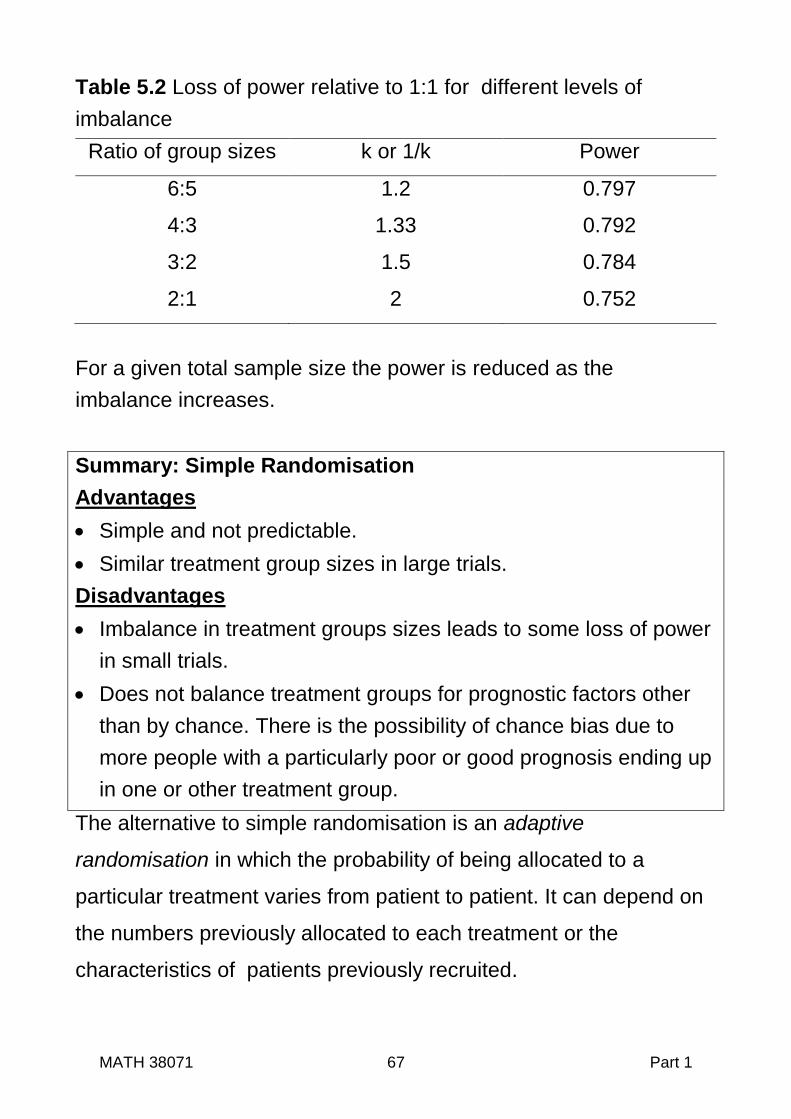
Table 5.2 Loss of power relative to 1:1 for different levels of
imbalance
Ratio of group sizes k or 1/k Power
6:5 1.2 0.797
4:3 1.33 0.792
3:2 1.5 0.784
2:1 2 0.752
For a given total sample size the power is reduced as the
imbalance increases.
Summary: Simple Randomisation
Advantages
Simple and not predictable.
Similar treatment group sizes in large trials.
Disadvantages
Imbalance in treatment groups sizes leads to some loss of power
in small trials.
Does not balance treatment groups for prognostic factors other
than by chance. There is the possibility of chance bias due to
more people with a particularly poor or good prognosis ending up
in one or other treatment group.
The alternative to simple randomisation is an adaptive
randomisation in which the probability of being allocated to a
particular treatment varies from patient to patient. It can depend on
the numbers previously allocated to each treatment or the
characteristics of patients previously recruited.

MATH 38071 68 Part 1
5.2 Blocks Randomisation
Block Randomisation, also referred to as Randomised Permuted
Blocks, aims to keep treatment group sizes in a particular ratio,
which is usually 1:1. Blocks of treatment allocations are created
with each block containing the treatments in the required ratio.
Blocks are then randomly selected to construct a randomisation list.
All the treatment allocations on the list are then used in sequence
as patients are recruited.
Procedure for Block Randomisation
1. Suppose the number of treatments being compared is N. Choose
a block length L (>N). With equal allocations this must be an
integer multiple of the number of treatments being compared, say
N.
2. All sequences of treatment allocations for the chosen block size
are then enumerated. For a block size L with N treatments, the
number of unique blocks is
!
!N
LP
M
where M=L/N assuning
equal allocation ratio.
3. Select a sequence of numbers between 1 and P at random from
random number tables or equivalent.
4. Assemble a randomisation list by selecting the blocks according
to the sequence of random numbers.
5. Patients are then allocated in turn according to the list.

MATH 38071 69 Part 1
Ex5.1 Assuming equal allocation is required, create a
randomisation list of 20 patients for a trial with two treatments using
block randomisation with a block size of four and the random
number sequence 1, 6, 3, 1, 4.
L= and N = gives P unique blocks .
Using the labels A and B for the two treatment the unique blocks
are
The blocks can then be chosen using the random number
sequence and added to the table create the randomisation list.
Table 5.3 Randomisation list constructed using block randomisation Patient
Num 1 2 3 4 5 6 7 8 9
1
0
1
1
1
2
1
3
1
4
1
5
1
6
1
7
1
8
1
9
2
0
Block
Treat.

MATH 38071 70 Part 1
Summary: Block Randomisation
Advantages compared to Simple Randomisation
Reduces imbalance in group sizes. For two groups with block
length L and allocation ratio of (1:1) the maximum imbalance
during the trial is L/2 and group sizes are balanced at the end of
each block.
Prevents bias due to secular (time) trends in prognosis of patient
recruited as similar proportions of each treatment are allocated in
each time period of the trial.
Disadvantages
More complicate than simple randomisation.
With a small block length it may be possible to predict the next
allocation. For this reason a block size of 2 is never used. One
way to reduce predictability is to use a random mixture of block of
different sizes. e.g. for two treatments use blocks of sizes 4, 6
and 8.

MATH 38071 71 Part 1
5.3 Allocation and Prognostic Factors Block randomisation only balances the design with respect to size.
As with simple randomisation, it does not balance treatment groups
for prognostic factors. By chance, the composition of the two groups
may differ. For example, suppose a small proportion of eligible
patients have a particularly poor or good prognosis. From the table
5.1 it can be seen that these could be unequally distributed
between treatment arms, causing chance bias.
Since it is desirable to have treatment groups that have a similar
composition in terms of important prognostic factors, it makes
sense to vary the allocation probability to achieve this. Two
methods that allow this are Stratified Randomisation and
Minimization. Nevertheless block randomisation is still relevant, as it
is required for stratified randomisation.
Stratified Randomisation
A small number of prognostic factors can be balanced using this
form of randomisation by using different block randomisations for
groups or strata of patients. Before the trial begins strata need to
be defined either by a categorical variable such as gender or by
dividing a continuous variable such as age into bands.

MATH 38071 72 Part 1
Procedure for Stratified Randomisation
1. Select a categorical variable that defines the strata e.g. age
banding (-64, 65-74,75+)
2. Construct separate randomisation list for each strata using block
randomisation.
Stratification may be extended to two or more factors but the
number of block randomisation lists required rapidly becomes large.
For example 3 factors each with just 2 levels would requires 32 8
separate lists. As well as the added complexity, with many lists
there may be many incomplete blocks to be left at the end of the
trial that could cause imbalance unless the trial is large.
Note that if simple randomisation is used to prepare the list for each
strata in place of block randomisation, the benefit of stratified
randomisation is lost, as this will be no different to simple
randomisation.
Summary Stratified Randomisation
Advantages
Balances groups on prognostic factors used to stratify.
Disadvantages
More complex to organize and administer, which could lead to
mistakes.
Only feasible with a small number of strata / prognostic factors.

MATH 38071 73 Part 1
Minimisation
To carry out minimization one begins by selecting the factors we
wish to control. These need to be categorical variable or converted
into such by banding.
There are two type of minimization, deterministic and stochastic, the
difference between which is explained below.
Procedure for Minimisation
1. For each levels of each factor being controlled, a running total is
kept for the numbers of parents assigned to each treatment.
2. When a new patient is recruited, the totals for that patient’s
characteristic are added together for each treatment group. The
patient is then assigned to
(i) the treatment group with smaller total.
(deterministic minimization)
or
(ii) probabilistically using a larger probability (say 0.6 or 0.7)
for the treatment group with the smaller total.
(stochastic minimization)
3. After each patient is entered into the trial, the relevant totals for
each factor are updated based on the treatment allocation that
took place, ready for the next patient.
MATH 38071 74 Part 1
4. If totals are equal, simple randomisation is used. Hence, the first
patient is allocated using simple randomisation as all totals are
zero at the start of the trial.
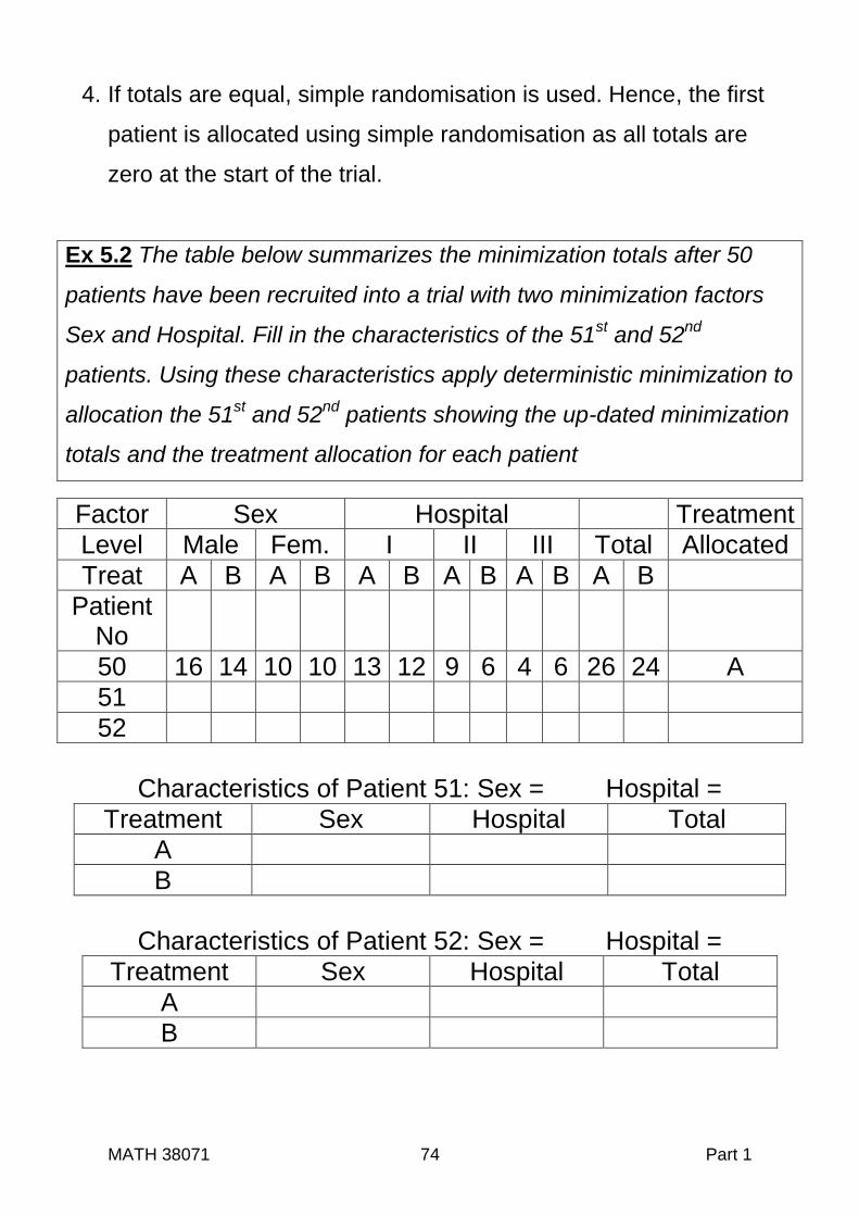
Ex 5.2 The table below summarizes the minimization totals after 50
patients have been recruited into a trial with two minimization factors
Sex and Hospital. Fill in the characteristics of the 51st and 52
nd
patients. Using these characteristics apply deterministic minimization to
allocation the 51st and 52
nd patients showing the up-dated minimization
totals and the treatment allocation for each patient
Factor Sex Hospital Treatment
Level Male Fem. I II III Total Allocated
Treat A B A B A B A B A B A B
Patient No
50 16 14 10 10 13 12 9 6 4 6 26 24 A
51
52
Characteristics of Patient 51: Sex = Hospital =
Treatment Sex Hospital Total
A
B
Characteristics of Patient 52: Sex = Hospital =
Treatment Sex Hospital Total
A
B

MATH 38071 75 Part 1
We have used deterministic minimisation in this example for
illustrative purposes, but deterministic minimization can be
predictable based on knowledge of previous allocations. Stochastic
minimisation is recommended but this is complicate without
specialist software.
Summary: Minimization
Advantages
Balance can be achieved on a larger set of prognostic factors
than for stratified randomisation.
Disadvantages
Complicated as randomisation list cannot be prepared in
advance but depend on the characteristics of patients as they are
recruited to the trial. It is tedious to do without specialist software.
Comparison of Stratified Randomisation and Minimization
Stratified randomisation maintains balance on all combinations of
factors. If a study is stratified on say gender and severity (mild,
severe), balance between treatments would be maintained on each
four combinations (male & mild), (male & severe), (female & mild)
and (female & severe).
Minimisation maintains balance between treatments for each level
of a factor but not on combinations of factors.

MATH 38071 76 Part 1
6. Statistical Analysis Using
Baseline Measurements

MATH 38071 77 Part 1
6.1 Baseline Data in Clinical Trials
In most clinical trials data is collected on the characteristics of
patients in addition to the outcome measures. As well as recording
demographic data such as age and sex, information will be
collected regarding the clinical status of the patient at the time of
entry into the trial, which could include values of the trial outcome
measures at entry into the trial. For example in a trial comparing
treatments for osteoarthritis of the knee, one might record
information regarding pain, physical impairment or psychological
distress, on entry into the trial . Such data may be required to
confirm that patients satisfy the inclusion criteria for the trial. It is
also used to describe the characteristic of patients entering the trial.
Standard practices would be to present a table summarizing the
characteristics for each treatment group.
Data collected prior to randomisation are called baseline data.
This data can also be used in the estimation and testing hypotheses
regarding the treatment effect. As we shall see, for just one
outcome measure, there are several ways in which this can be
done. If these are all carried out and the investigator allowed to
choose on the basis of the results, it is likely that the most
favourable will be presented. Alternatively, all could will be
presented, which could be a problem, if they give conflicting results.
Either way, this could distort the published report and would be a
source of statistical analysis bias. To prevent this the choice of

MATH 38071 78 Part 1
analysis should not be based on the results of the analyses of the
trial, but need to be documented in advance in a statistical analysis
plan. To do this we require criteria to make the decision in advance
as to which method of analysis should be used .
Ex 6.1 The FAP Trial Data
FAP is a genetic defect that predisposes those affected to develop
large numbers of polyps in the colon that are prone to become
malignant. In this trial patients with FAP were randomly allocated to
receive a drug therapy (sulindac) or a placebo.
Patient Treatment Polyp Size ID Group Baseline (X) 12 Months (Y)
1 sulindac 5.0 1.0 2 placebo 3.4 2.1 3 sulindac 3.0 1.2 4 placebo 4.2 4.1 5 sulindac 2.2 3.3 6 placebo 2.0 3.0 7 placebo 4.2 2.5 8 placebo 4.8 4.4 9 sulindac 5.5 3.5
10 sulindac 1.7 0.8 11 placebo 2.5 3.0 12 placebo 2.3 2.7 13 placebo 2.4 2.7 14 sulindac 3.0 4.2 15 placebo 4.0 2.9 16 placebo 3.2 3.7 17 sulindac 3.0 1.1 18 sulindac 4.0 0.4 19 sulindac 2.8 1.0
Piantadosi S. Clinical Trials: A methodological Perspective p302 , Wiley 1997

MATH 38071 79 Part 1
6.2 Possible Treatment Effect Estimators
(i) Unadjusted
Suppose the random variable Yi represents the continuous
outcome for the ith patient in either the new treatment group (T) or
the control group (C), and suppose
i U iY for i C
i U U iY for i T
with a random variable with | | 0i T i Ci iE E .
| |i T i CU i iE Y E Y ,
which can be estimated by
U T CY Y
(ii) Changes Scores
Suppose iX is the value of outcome measure iY recorded at
baseline. Medical researchers sometimes calculate the change
from baseline, i i iC Y X , which is call the change score.
Treatments are compared using iC instead of iY .
i i i C iC Y X for i C
i i i C C iC Y X for i T
with a random variable with | | 0i T i Ci iE E .
| |i T i CC i iE C E C ,
which can be estimated by

MATH 38071 80 Part 1
C T C T T C CC C Y X Y X
where TC and CC are the sample means of the change score for
each group.
For both these methods of analysis statistical inference can be
based on the two-sample t-test and the associated confidence
interval.
Figure 6.1 STATA Output for FAP trial (i) Unadjusted Analysis Two-sample t test with unequal variances
------------------------------------------------------------------------------
Group | Obs Mean Std. Err. Std. Dev. [95% Conf. Interval]
---------+--------------------------------------------------------------------
Sulindac | 9 1.833333 .4711098 1.413329 .7469522 2.919714
Placebo | 10 3.110000 .2306753 .7294595 2.588176 3.631824
---------+--------------------------------------------------------------------
diff | -1.276667 .5245527 .130485 2.422848
------------------------------------------------------------------------------
diff = mean(Sulindac)- mean(Placebo) t = -2.4338
Ho: diff = 0 Satterthwaite's degrees of freedom = 11.6981
Ha: diff < 0 Ha: diff != 0 Ha: diff > 0
Pr(T < t) = 0.0160 Pr(|T| > |t|) = 0.0320 Pr(T > t) =0.9840
(ii) Change Score Analysis
Two-sample t test with unequal variances
------------------------------------------------------------------------------
Group | Obs Mean Std. Err. Std. Dev. [95% Conf. Interval]
---------+--------------------------------------------------------------------
Sulindac | 9 -1.522222 .5969314 1.790794 -2.898749 -.1456959
Placebo | 10 -.1900000 .2857544 .9036346 -.8364213 .4564213
---------+--------------------------------------------------------------------
diff | -1.332222 .6618026 -.1160118 2.780456
------------------------------------------------------------------------------
diff = mean(Sulindac)- mean(Placebo) t = -2.0130
Ho: diff = 0 Satterthwaite's degrees of freedom = 11.5476
Ha: diff < 0 Ha: diff != 0 Ha: diff > 0
Pr(T < t) = 0.0340 Pr(|T| > |t|) = 0.0680 Pr(T > t) =0.9660
Note: Adjusted degrees of freedom have been used in both
analyses. This method, called the Satterthwaite test and mention in
2.2, adjusts inference for variance of the two arms being unequal.

MATH 38071 81 Part 1
(iii) Analysis Adjusted by Baseline Variables
Suppose that X is a baseline variable. Suppose for some values
we define an adjusted treatment effect as
i i i A iA Y X for i C
i i i A iA Y X for i T
with i a random variable with | | 0i T i Ci iE E .
Taking expectations,
| |i T i Ci i i iE Y X E Y X ,
which can be estimated by
ˆT C T T C CA A Y X Y X
For simplicity it will be assumed that X is a single variable, but it
could be a vector of covariates.
Baseline variables can be binary or continuous. If X is a binary
variable, it is generally convenient to code it with 0 and 1. A
variable coded in this way is sometimes called an indicator or
dummy variable.

MATH 38071 82 Part 1
6.3 Comparison of Adjusted and Unadjusted Analyses
In a randomised controlled trial ˆE is independent of
. Hence the expected values of unadjusted, change and an
adjusted estimate of the treatment effect are all equal, that is
ˆ ˆ ˆU CE E E
Proof
Considering T T C CY X Y X .
ˆT C T CE E Y E Y E X E X .
Randomisation means that CT XEXE .
Therefore ˆT CE E Y E Y , which is independent of .
Values of equal to 0 and 1 correspond to the treatment effect in
an unadjusted U , and change C giving the required result ■

MATH 38071 83 Part 1
Suppose 2 2, ,X Y XY are the variances and covariance of X and Y
with CT nn
11 . The treatment effect ˆA has a minimum variance
when equal to 2 2 2ˆ 1YVar where is the
regression coefficient of Y on X and is the correlation between X
and Y conditional on treatment group.
Proof
Again consider ˆT T C CY X Y X
ˆT C T CVar Var Y Y X X
2 ,T C T C T C T CVar Y Y Var X X Cov Y Y X X
2. 2 . ,T C T C T C T CVar Y Y Var X X Cov Y Y X X [1]
Considering the first term
2 ,T C T C T CVar Y Y Var Y Var Y Cov Y Y .
Since treatment groups are independent, , 0T CCov Y Y .
Therefore T C T CVar Y Y Var Y Var Y .
Since observations are independent,
2
YT
T
Var Yn
and
2
YC
C
Var Yn
.
Therefore 2 2
T C YVar Y Y where CT nn
11 .

MATH 38071 84 Part 1
Similarly 22
XCT XXVar and 2,T C T C XYCov Y Y X X .
Substitution into [1] gives 2 2 2 2ˆ 2y X XYVar [2]
A minima can be found by differentiation with respect to .
2 2ˆ 2 2X XYVar
.
This equals zero when 2
XY X , which is the coefficient for
regression of Y on X within each treatment group.
The second derivative 2
2 2
2ˆ 2 XVar
.
As this is positive, it follows that this is a minimum. The treatment
effect estimate with minimum variance is therefore
2
2 2 2 2 2 2
2 2ˆ 2 1 XY
Y X XY Y
X Y
Var
Since 2 2
XY X y , 2 2 2ˆ 1YVar as required ■

MATH 38071 85 Part 1
Estimation of and
The treatment effect can be estimated by fitting a linear
model, which is a generalization of linear regression. The general
form of a linear model with k covariates is
1 1 ...i i k ki iY X X .
where the X’s are the k covariates and the ’s the corresponding k
coefficients. The random variable i is usually assumed to be
20,N . If one of the X’s is an indicator variable, the coefficient 𝛽
is the difference in the mean value of Y for X =1 as compared to
X=0 , adjusted for other X’s.
When considering the analysis of data from a randomised trial it is
notational clearer to separate the matrix of covariates into an
indicator variable Ii equal to 1 for treatment T and 0 for the control
C, and a matrix X of other covariates. The model is then written as
i A i i iY I X
and the treatment effect is the coefficient of the indicator variable Ii.
Statistical inference is simply the test of whether the coefficient of
the indicator variable Ii differs from zero, that is 0: 0 H vs
1: 0 H . The matrix of coefficients, , for other variable is
generally of less interest and often not given in published reports of
trials.

MATH 38071 86 Part 1
Fig 6.2 STATA Output for FAP trial Linear Model Analysis Adjusting for Baseline Polyp Size Source | SS df MS Number of obs = 19
-------------+------------------------------ F( 2, 16) = 3.48
Model | 8.63531123 2 4.31765562 Prob > F = 0.0556
Residual | 19.8541618 16 1.24088511 R-squared = 0.3031
-------------+------------------------------ Adj R-squared = 0.2160
Total | 28.4894731 18 1.5827485 Root MSE = 1.114
size12 | Coef. Std. Err. T P>|t| [95% Conf. Interval]
-------------+----------------------------------------------------------------
size0 | .2087081 .243071 0.86 0.403 -.3065794 .7239956
treatment | -1.288262 .5120029 -2.52 0.023 -2.373659 -.2028639
_cons | 2.421263 .8760753 2.76 0.014 .5640666 4.27846
-------------+----------------------------------------------------------------
Table 6.2 summarizes the treatment effect and inference for all
three analyses. The null hypothesis of no treatment effect would not
have been rejected at a 5% level if the change score analysis had
been carried out.
Table 6.2 Summary of treatment effect estimates for the FAP trial
Treatment Effect
SE 95% Lower
C.I Upper
p-value
Unadjusted U -1.28 0.52 -2.42 -0.13 0.032
Change ˆC -1.33 0.66 -2.78 0.12 0.068
Linear Model
-1.29
0.51 -2.37 -0.20 0.023
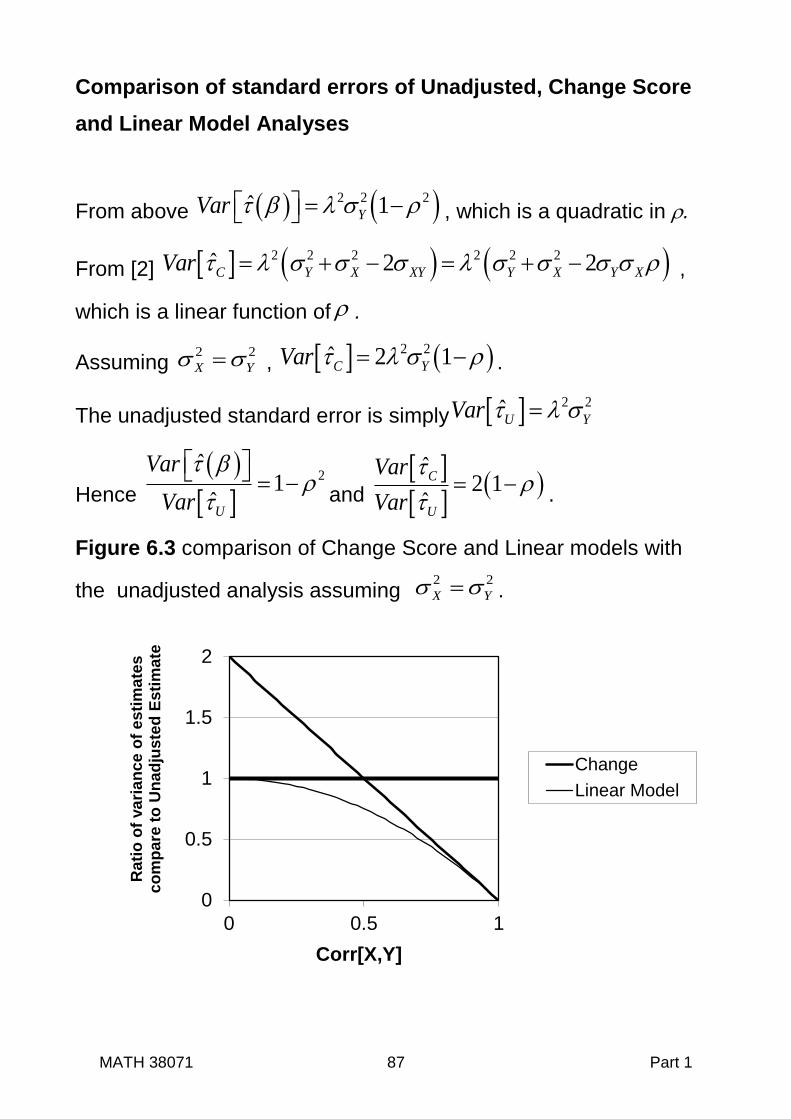
MATH 38071 87 Part 1
Comparison of standard errors of Unadjusted, Change Score
and Linear Model Analyses
From above 2 2 2ˆ 1YVar , which is a quadratic in .
From [2] 2 2 2 2 2 2ˆ 2 2C Y X XY Y X Y XVar ,
which is a linear function of .
Assuming 2 2
X Y , 2 2ˆ 2 1C YVar .
The unadjusted standard error is simply 2 2
U YVar
Hence
2
ˆ1
U
Var
Var
and
ˆ
2 1ˆ
C
U
Var
Var
.
Figure 6.3 comparison of Change Score and Linear models with
the unadjusted analysis assuming 2 2
X Y .
0
0.5
1
1.5
2
0 0.5 1
Rati
o o
f va
ria
nce
of
es
tim
ate
s
co
mp
are
to
Un
ad
juste
d E
sti
ma
te
Corr[X,Y]
Change
Linear Model

MATH 38071 88 Part 1
Summary Analyses using Baseline Data
All three estimates of the treatment effect defined in (6.2) are
unbiased, but an estimate of the treatment effect based on a linear
model has smaller expected variance, where baseline covariates
correlate with the outcome measure and it does not matter whether
this correlation is positive or negative.
Reducing the variance of the treatment effect estimate is important
as this increases the precision of the estimate, thereby giving
greater power for a given sample size. As a consequence, if a
baseline variable is thought to predict outcome, an analysis
adjusting for this variable is recommended. Where an outcome
measure is recorded at baseline, then it is usually a strong predictor
of outcome, and the variable should be used as a covariate.
To prevent the analysis bias, a single set of baseline covariates
should be selected prior to starting analysis. This should be
recorded in the statistical analysis plan of the trial. This choice will
therefore need to be based on prior knowledge or reasoning as to
what variables are likely to predict outcome irrespective of which
treatment is received.

MATH 38071 89 Part 1
6.4 A Flawed Analysis using Within Group Change from Baseline
A statistical analysis sometime seen in the medical literature is to
carry out a separate paired t-test on each treatment groups.
Treatments are then compared by using the results of the separate
statistical tests. If improvement in one group is statistically
significant but not the other, it is concluded that one treatment is
more effective than the other. This analysis is illustrated below with
the FAP data
Figure 6.4 STATA Output for paired t-test analysis of each treatment Results for: polyp.mtw (treat = 0) Paired t test
------------------------------------------------------------------------------
Variable | Obs Mean Std. Err. Std. Dev. [95% Conf. Interval]
---------+--------------------------------------------------------------------
size12 | 10 3.11 .2306753 .7294595 2.588176 3.631824
size0 | 10 3.3 .3076795 .972968 2.603981 3.996019
---------+--------------------------------------------------------------------
diff | 10 -.19 .2857544 .9036346 -.8364213 .4564213
------------------------------------------------------------------------------
mean(diff) = mean(size12 - size0) t = -0.6649
Ho: mean(diff) = 0 degrees of freedom = 9
Ha: mean(diff) < 0 Ha: mean(diff) != 0 Ha: mean(diff) > 0
Pr(T < t) = 0.2614 Pr(|T| > |t|) = 0.5228 Pr(T > t) = 0.7386
Results for: polyp.mtw (treat = 1) Paired t test
------------------------------------------------------------------------------
Variable | Obs Mean Std. Err. Std. Dev. [95% Conf. Interval]
---------+--------------------------------------------------------------------
size12 | 9 1.833333 .4711098 1.413329 .7469522 2.919714
size0 | 9 3.355556 .4163703 1.249111 2.395404 4.315707
---------+--------------------------------------------------------------------
diff | 9 -1.522222 .5969314 1.790794 -2.898749 -.1456959
------------------------------------------------------------------------------
mean(diff) = mean(size12 - size0) t = -2.5501
Ho: mean(diff) = 0 degrees of freedom = 8
Ha: mean(diff) < 0 Ha: mean(diff) != 0 Ha: mean(diff) > 0
Pr(T < t) = 0.0171 Pr(|T| > |t|) = 0.0342 Pr(T > t) = 0.9829

MATH 38071 90 Part 1
Why the Analysis using Within-Group Changes is Flawed
The main reason why this method is flawed is because the two p-
values relate to two separate hypotheses test and so do not directly
test the benefit of one treatment as compared to the other, that is
they do not compare the two potential outcomes.
Use of this type of analysis also suggests other misunderstandings.
Failure to reject the null hypothesis, for a treatment does not
imply that there is no change. The absolute change within each
treatment groups could be the same but unequal variances may
affect the probability of rejecting the null hypothesis for one
treatment and not another.
Tests of within group change are often statistically significant, but
change within a treatment group may not be due to treatment. It
may occur because the condition naturally resolves. They may
tell us more about the natural history of the condition than the
benefit of receiving treatment one treatment as compared to
another.
Unfortunately, clinical researchers often carry out this type of
analysis, when the statistical analysis directly comparing the two
treatments is not statistically significant. This is done in the
desperate search for a statistically significant result to report.