Mechanisms for the Maintenance of the Wintertime Basin-Scale Atmospheric Responseto Decadal SST Variability in the North Pacific Subarctic Frontal Zone

SATORU OKAJIMA,a HISASHI NAKAMURA,a,b KAZUAKI NISHII,c TAKAFUMI MIYASAKA,a

AKIRA KUWANO-YOSHIDA,d BUNMEI TAGUCHI,a MASATO MORI,a AND YU KOSAKAa

aResearch Center for Advanced Science and Technology, The University of Tokyo, Tokyo, JapanbApplication Laboratory, JAMSTEC, Yokohama, Japan

cGraduate School of Bioresources, Mie University, Tsu, JapandDisaster Prevention Research Institute, Kyoto University, Shirahama, Japan

(Manuscript received 28 March 2017, in final form 4 October 2017)

ABSTRACT

Mechanisms for the maintenance of a large-scale wintertime atmospheric response to warm sea surface

temperature (SST) anomalies associated with decadal-scale poleward displacement of the North Pacific sub-

arctic frontal zone (SAFZ) are investigated through the following two ensemble experiments with an atmo-

spheric general circulation model (AGCM): one with climatological-mean SST and the other with positive SST

anomalies along the SAFZ prescribed on top of the climatological-mean SST. As actually observed, the sim-

ulated January ensemble response over the North Pacific is anticyclonic throughout the depth of the tropo-

sphere, although its amplitude is smaller. This response is maintained through energy conversion from the

ensemble climatological-mean circulation realized under the climatological SST as well as feedback from

anomalous transient eddy activity, suggesting that the response may have characteristics as a preferredmode of

variability (or ‘‘dynamical mode’’). Conversions of both available potential energy and kinetic energy from the

climatological-mean state are important for the observed anomaly, while the latter is less pronounced for the

model response. Net transient feedback forcing is also important for both the observed anomaly and simulated

response. These results imply that a moderate-resolution (;18) AGCM may be able to simulate a basin-scale

atmospheric response to the SAFZ SST anomaly through synoptic- and basin-scale dynamical processes.

Weaker PNA-like internal variability in the model may lead to the weaker response, suggesting that mis-

representation of intrinsic atmospheric variability can affect the model response to the SST anomaly.

1. Introduction

Owing to greater persistence of SST anomalies than

atmospheric anomalies, a robust atmospheric response

to oceanic forcing, if any, could contribute to improve-

ment in seasonal forecast skill. Influence of extratropical

SST anomalies on the large-scale atmospheric circula-

tion has long been believed to be insignificant, in the

presence of a prevailing remote influence from the

tropics (Lau 1997; Alexander et al. 2002) and large in-

trinsic atmospheric variability (Frankignoul 1985;

Kushnir et al. 2002). Over decades, a number of studies

have strived to assess atmospheric responses to pre-

scribed midlatitude SST anomalies by using various at-

mospheric general circulation models (AGCMs) with

SST anomalies imposed over different regions (e.g., Lau

and Nath 1990; Kushnir and Lau 1992; Peng et al. 1995,

1997; Lau 1997). Peng et al. (1997) and Peng and

Whitaker (1999) suggested that a large-scale AGCM

response to the prescribed SST anomaly is sensitive to its

relative position to the background westerlies simulated

in the AGCM, as confirmed by Kushnir et al. (2002). In

fact, Robinson (2000) reported difficulties in AGCM

experiments in obtaining systematic atmospheric re-

sponses to positive and negative SST anomalies pre-

scribed in the midlatitudes.

To assess the importance of midlatitude SST vari-

ability in forcing wintertime basin-scale atmospheric

anomalies, recent studies have been focusing on persis-

tent SST anomalies in the North Pacific subarctic frontal

zone (SAFZ), taking advantage of satellite measure-

ments, newer models, and longer observational data.

The North Pacific SAFZ forms a boundary between theCorresponding author: Satoru Okajima, okajima@atmos.rcast.

u-tokyo.ac.jp

1 JANUARY 2018 OKA J IMA ET AL . 297

DOI: 10.1175/JCLI-D-17-0200.1

� 2018 American Meteorological Society. For information regarding reuse of this content and general copyright information, consult the AMS CopyrightPolicy (www.ametsoc.org/PUBSReuseLicenses).

Unauthenticated | Downloaded 04/06/22 01:52 AM UTC

warm Kuroshio and cool Oyashio waters (Yasuda 2003;

Kida et al. 2015) with a climatologically sharp meridio-

nal SST gradient and vigorous atmosphere–ocean in-

teraction (Kwon et al. 2010; Kelly et al. 2010; Nakamura

et al. 2015). The sharp meridional SST gradient across

the SAFZ was unresolved in AGCMs used in the

aforementioned studies, because of their rather coarse

horizontal resolution. Tanimoto et al. (2003) and

Taguchi et al. (2009, 2012) have found that, unlike in

most of the North Pacific basin where surface heat flux

anomalies due to changes in near-surface wind, air

temperature, and humidity force SST anomalies, warm

(cold) SST anomalies along the SAFZ tend to enhance

(reduce) heat release into the atmosphere, which can be

regarded as thermodynamic forcing by the SAFZ vari-

ability on the overlying atmosphere. In fact, using linear

inverse modeling, Smirnov et al. (2014) suggested that a

substantial fraction (;50%) of the wintertime monthly

SST variability is intrinsic to the ocean over the North

Pacific western boundary current region, while much of

the variability in other regions arises from atmospheric

forcing on the ocean. It is thus worth investigating the

persistent large-scale atmospheric response to the

SAFZ SST variability.

Meridional displacement of the SAFZ, which is due to

incoming oceanic Rossby waves, yields meridionally

confined persistent SST anomalies (Seager et al. 2001;

Schneider et al. 2002; Nonaka et al. 2006; Taguchi et al.

2007; Newman et al. 2016). Indeed, decadal SST vari-

ability in winter exhibits a primarymaximum off the east

coast of Japan along the SAFZ and a secondary maxi-

mum over the subtropical frontal zone (Nakamura and

Kazmin 2003). The SST variability in SAFZ exhibits no

significant simultaneous correlation with the tropical

SST variability, suggesting that the former variability is

inherent to the North Pacific (Taguchi et al. 2012), while

the SST over the subtropical frontal zone varies in see-

saw with the tropical SST (Nakamura et al. 1997).

Nakamura et al. (1997) have shown that wintertime

decadal SST anomalies in the SAFZ tend to accompany

persistent anomalies in the surface Aleutian low and

upper-level anomalies that closely resemble the Pacific–

North American (PNA) pattern (Wallace and Gutzler

1981). Since then, the relationship between SST anom-

alies associated with oceanic fronts and large-scale at-

mospheric anomalies has been investigated. Focusing on

the Kuroshio Extension, Joyce et al. (2009) suggested

from atmospheric reanalysis data that the surface storm-

track axis shifts meridionally following a decadal dis-

placement of the SAFZ. O’Reilly and Czaja (2015) also

pointed out that when the Kuroshio Extension is less

meandering, atmospheric heat transport by transient

eddies increases over the western North Pacific.

Frankignoul et al. (2011) found that persistent dipole-

like atmospheric anomalies, which are uncorrelated

with SST variability in the tropics, tend to emerge in

association with a meridional shift of the Oyashio front.

Kwon and Joyce (2013) also revealed that the northward

shift of the SAFZ leads to the suppression of the storm-

track activity in the North Pacific. Analyzing observa-

tional data and a long-term coupled ocean–atmosphere

general circulationmodel (CGCM) integration, Taguchi

et al. (2012) revealed that late-autumn warming around

the SAFZ due to its northward shift forces the persistent

weakening of the Aleutian low, which peaks in January

and decays rapidly through February. As suggested by

Newman et al. (2016), the aforementioned covariability

between SST anomalies in the SAFZ and large-scale

atmospheric anomalies may constitute a feedback loop

to contribute to the so-called Pacific decadal variability.

Those findings are based on observational data

analysis and a coupled model experiment. Anomalies

in a coupled system are a mixture of the atmospheric

forcing pattern onto a given SST anomaly and a re-

sponse to it, and the anomalies can therefore be influ-

enced by forcings other than the SAFZ SST anomalies

as well as atmospheric internal variability. While an

exact match between the observed anomalies and

AGCM response is therefore not expected, AGCM

experiments can extract a response to the SAFZ SST

anomalies, which would substantiate the aforemen-

tioned findings on oceanic forcing to the large-scale

atmospheric circulation.

In a recent study, Smirnov et al. (2015) compared

large-scale atmospheric responses obtained in a pair of

experiments with different horizontal resolutions of

a state-of-the-art AGCM. In their higher-resolution

(0.258 3 0.258) experiment, a robust basin-scale anticy-

clonic response is simulated throughout the depth of the

troposphere to a warm SST anomaly prescribed only

within the SAFZ, while such a deep response disappears

in their lower-resolution (1.08 3 1.08) experiment, which

simulates a lower-tropospheric cyclonic response only.

They stressed the importance of mesoscale atmospheric

perturbations in forcing the high-resolution (and thus

more realistic) response. However, the aforementioned

work by Taguchi et al. (2012) presented deep anticy-

clonic anomalies in association with the northward shift

of the SAFZ in a long-term integration of a CGCM

with a modest atmospheric resolution of 1.08 3 1.08,motivating the reexamination of the atmospheric re-

sponse to the SAFZ variability with a modest resolution

(;18) AGCM. In fact, an AGCM ensemble experiment

by Okajima et al. (2014) successfully reproduced a per-

sistent basin-scale anticyclonic anomaly observed in

October 2011 as a robust response to an extreme warm

298 JOURNAL OF CL IMATE VOLUME 31

Unauthenticated | Downloaded 04/06/22 01:52 AM UTC

SST anomaly in the SAFZ. These two studies with the

horizontal resolution of the atmospheric model being

about 1.08 suggest that synoptic and basin-scale pro-

cesses, in addition to mesoscale processes, can be of

particular importance for maintaining the basin-scale

response, a hypothesis that is tested by the present study.

This paper is organized as follows. Section 2 describes

the data and experimental design. Section 3 compares

observed anomalies and the corresponding AGCM

responses, followed by discussions on maintenance

mechanisms. Section 4 gives a summary and additional

discussions.

2. Data and numerical experiments

a. Observational data

Atmospheric variables, including sea level pressure

(SLP), geopotential height, air temperature, horizontal

wind and pressure velocity, diabatic heating rates, and

surface turbulent heat fluxes are obtained from the new

Japanese 55-year Reanalysis of the global atmosphere

(JRA-55; Kobayashi et al. 2015; Harada et al. 2016) for

the period 1958–2010 available on a 1.258 3 1.258 grid. Inaddition, the following two SST datasets are used. One is

the climatological-mean SST field for each calendar

month derived from the National Oceanic and Atmo-

spheric Administration (NOAA) Optimum Interpola-

tion Sea Surface Temperature (OISST), into which SST

data from satellite observations and in situ observations

are blended since November 1981 (Reynolds et al.

2007). Assigned on a 0.258 3 0.258 grid, the data can

resolve the finescale structure of the SAFZ. Meanwhile,

anomalous SST fields associated with the decadal-scale

SAFZ variability have been derived from in situ surface

marine observations by ships and buoys that have been

compiled in the International Comprehensive Ocean

Atmosphere Dataset (ICOADS; Worley et al. 2005) for

the period 1960–2011. Thanks to its longer data period,

ICOADS can cover both the prominent positive and

negative events of the decadal-scale SAFZ variability

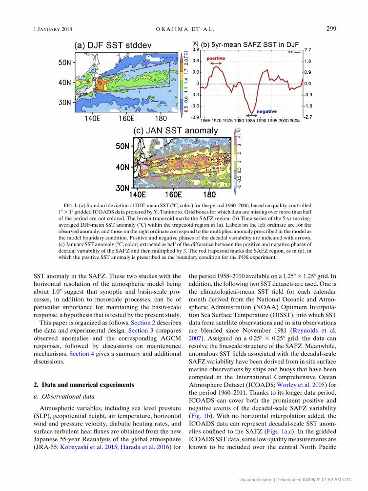
(Fig. 1b). With no horizontal interpolation added, the

ICOADS data can represent decadal-scale SST anom-

alies confined to the SAFZ (Figs. 1a,c). In the gridded

ICOADS SST data, some low-quality measurements are

known to be included over the central North Pacific

FIG. 1. (a) Standard deviation ofDJF-mean SST (8C; color) for the period 1960–2006, based on quality-controlled18 3 18 gridded ICOADS data prepared byY. Tanimoto. Grid boxes for which data aremissing over more than half

of the period are not colored. The brown trapezoid marks the SAFZ region. (b) Time series of the 5-yr moving-

averaged DJF-mean SST anomaly (8C) within the trapezoid region in (a). Labels on the left ordinate are for the

observed anomaly, and those on the right ordinate correspond to themultiplied anomaly prescribed in themodel as

the model boundary condition. Positive and negative phases of the decadal variability are indicated with arrows.

(c) January SST anomaly (8C; color) extracted as half of the difference between the positive and negative phases of

decadal variability of the SAFZ and then multiplied by 3. The red trapezoid marks the SAFZ region, as in (a), in

which the positive SST anomaly is prescribed as the boundary condition for the POS experiment.

1 JANUARY 2018 OKA J IMA ET AL . 299

Unauthenticated | Downloaded 04/06/22 01:52 AM UTC

(Minobe and Maeda 2005), which have been removed

through subjective quality control by Y. Tanimoto of

Hokkaido University (Tanimoto et al. 1997; Iwasaka

and Hanawa 1990).

b. AGCM experiments

The present study uses an AGCM for the Earth

Simulator (AFES; Ohfuchi et al. 2004, 2007; Enomoto

et al. 2008; Kuwano-Yoshida et al. 2010) with a hori-

zontal resolution of T119 spectral truncation (equiva-

lently 110-km grid intervals) and 56 vertical levels up to

the 0.1-hPa level. Though not particularly high, this

resolution is the same as that of the atmospheric com-

ponent of the CGCM used in Taguchi et al. (2012) and

typical among models used for climatic projection. With

this horizontal resolution, both the pronounced SST

gradient and meridionally confined SST anomalies in

the SAFZ, if prescribed as the model boundary condi-

tion, can be resolved reasonably well. In fact, the same

AGCM with the T119 truncation was successful in

reproducing a basin-scale anticyclonic anomaly ob-

served in October 2011 in response to SST anomalies

around the SAFZ, as shown in Okajima et al. (2014),

where details of AFES, including parameterization

schemes, are described.

A pair of ensemble experiments has been conducted

with AFES. One is a control experiment (CTRL), in

which AFES is forced with the climatological-mean

monthly SST and sea ice cover derived from OISST.

The other is the positive experiment (POS), for which

the SST field for AFES is constructed in such a way

that only the positive decadal SST anomaly observed

along the SAFZ has been added to the climatological-

mean field. In the present study, the SAFZ is marked

as the trapezoidal region (358–428N, 1408E and 388–508N, 1738W) in Fig. 1a, where the SST variability is

particularly large. In fact, the area-averaged SST

anomaly over the region clearly shows decadal vari-

ability in winter (Fig. 1b). The periods in which the 5-yr

mean of the area-averaged wintertime SST were

highest (from 1967/68 to 1971/72) and lowest (from

1983/84 to 1987/88) are defined as representative pe-

riods for the positive and negative phases of the de-

cadal SST variability. The SST anomaly for a given

calendar month is defined as half of the local difference

of ICOADS SST between the two epochs. Because the

purpose of this study is to examine the mechanisms for

maintaining a large-scale atmospheric response, which

requires a robust model response, the SST anomaly

(viz., half of the difference between the two epochs,

from 1967/68 to 1971/72 and from 1983/84 to 1987/88)

observed along the SAFZ has been multiplied by 3.

The SST anomaly assigned thus becomes as strong as

28–38C and comparable in magnitude to those actually

observed by satellites in October 2011 and prescribed

for the experiment by Okajima et al. (2014). The in-

flation of the SST anomaly may be justified in recog-

nition of the tendency for the ICOADS data to

underestimate the magnitude of SST anomalies as

measured by satellites. As an example, Fig. 1c shows

the SST anomaly in January prescribed for the POS

experiment.

Each of these two experiments (CTRL, POS) com-

prises 40 members, whose initial conditions were de-

rived from the model output simulated for 1 October

2011 of the individual ensemble members of the control

experiment by Okajima et al. (2014), whose initial

conditions were taken from the JRA-25 data (Onogi

et al. 2007) for individual days from 27 May to 5 June

2011. Ten members are integrated from the model

output on 1 October 2011. Another 10 members are

integrated with the same model executable file and ini-

tial conditions as the first 10 members, but on an up-

dated Earth Simulator system with newer processors.

Integrations on the two systems become diverse after a

few weeks as a result of the chaotic nature of the sim-

ulated atmosphere, and therefore we can consider them

as independent members. Yet, we have confirmed that

the ensemble-mean fields are similar between the two

sets. For another 20 members, initial conditions have

been obtained as the fields after integrating the 10 out-

puts on 1 October 2011 for one day or two. Each

member is integrated until the end of the subsequent

March, with daily SST fields interpolated linearly in time

from its monthly fields. Deviations of the ensemble-

mean atmospheric fields simulated in the POS experi-

ment from the CTRL counterpart are regarded as the

model atmospheric response to the positive SST

anomaly associated with the decadal SAFZ variability,

and their robustness is assessed locally by the t statistic.

In this paper, the January responses as well as observed

anomalies are investigated, which are strongest during

the winter.

The present study also utilizes the 120-yr CGCM in-

tegration analyzed by Taguchi et al. (2012). The coupled

model is the CGCM for the Earth Simulator (CFES),

consisting of AFES with horizontal resolution of T119

spectral truncation and 48 vertical levels up to the 1-hPa

level and the Coupled Ocean–Sea Ice Model for the

Earth Simulator (OIFES; Komori et al. 2005) with 0.58grid intervals and 54 vertical levels. Although mesoscale

oceanic eddies are unresolved with this configuration,

CFES can still simulate a prominent oceanic frontal

zone in the North Pacific that marks the boundary be-

tween the subtropical and subpolar gyres, which corre-

sponds to the SAFZ. Details of CFES, including

300 JOURNAL OF CL IMATE VOLUME 31

Unauthenticated | Downloaded 04/06/22 01:52 AM UTC

parameterization schemes, are described in Taguchi

et al. (2012).

3. Results

a. Structure of the circulation anomalies/responses inmidwinter

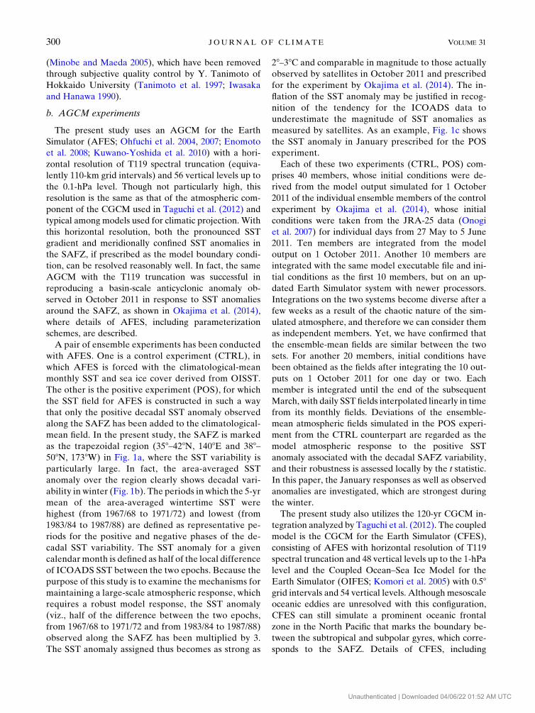
Figures 2a and 2b show maps of the January anoma-

lies of 300-hPa height (Z300) and SLP, respectively,

observed over the North Pacific as their differences

between the positive (1967/68–1971/72) and negative

(1983/84–1987/88) phases of the decadal SAFZ vari-

ability (Nakamura et al. 1997; Taguchi et al. 2012). In

these panels and hereafter, the magnitude of the ob-

served difference is halved, so as to represent the typical

amplitude of ‘‘anomalies’’ for the positive phase, which

is characterized by a positive SST anomaly in the SAFZ.

The remote influence from other ocean basins is con-

sidered to be weak (see appendix). Over the midlatitude

North Pacific, a well-defined basin-scale anticyclonic

anomaly was observed in both the lower and upper

troposphere, which resembles the PNA pattern defined

by Wallace and Gutzler (1981). The corresponding re-

sponse in the POS experiment is shown in Figs. 2c and

2d. Though weaker in magnitude and shifted slightly

southwestward, the upper-tropospheric anticyclonic

anomaly is simulated (Fig. 2c) as an ensemble response

to the warm SST anomaly in the SAFZ. In the lower

troposphere (Fig. 2d), however, the anticyclonic re-

sponse south of Alaska is not statistically significant,

while a cyclonic response simulated around Japan ex-

tends eastward over the warm SAFZ.

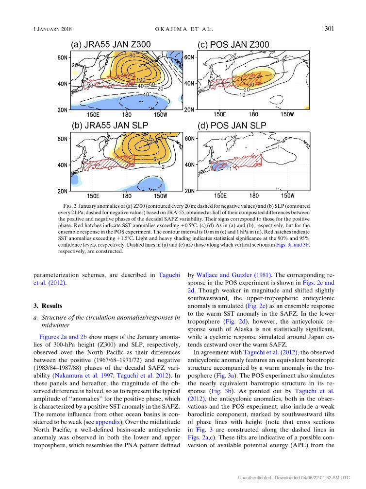
In agreement with Taguchi et al. (2012), the observed

anticyclonic anomaly features an equivalent barotropic

structure accompanied by a warm anomaly in the tro-

posphere (Fig. 3a). The POS experiment also simulates

the nearly equivalent barotropic structure in its re-

sponse (Fig. 3b). As pointed out by Taguchi et al.

(2012), the anticyclonic anomalies, both in the obser-

vations and the POS experiment, also include a weak

baroclinic component, marked by southwestward tilts

of phase lines with height (note that cross sections

in Fig. 3 are constructed along the dashed lines in

Figs. 2a,c). These tilts are indicative of a possible con-

version of available potential energy (APE) from the

FIG. 2. January anomalies of (a) Z300 (contoured every 20m; dashed for negative values) and (b) SLP (contoured

every 2 hPa; dashed for negative values) based on JRA-55, obtained as half of their composited differences between

the positive and negative phases of the decadal SAFZ variability. Their signs correspond to those for the positive

phase. Red hatches indicate SST anomalies exceeding 10.58C. (c),(d) As in (a) and (b), respectively, but for the

ensemble response in the POS experiment. The contour interval is 10m in (c) and 1 hPa in (d). Red hatches indicate

SST anomalies exceeding 11.58C. Light and heavy shading indicates statistical significance at the 90% and 95%

confidence levels, respectively. Dashed lines in (a) and (c) are those along which vertical sections in Figs. 3a and 3b,

respectively, are constructed.

1 JANUARY 2018 OKA J IMA ET AL . 301

Unauthenticated | Downloaded 04/06/22 01:52 AM UTC

climatological-mean temperature gradient into the

anomalies, as discussed later.

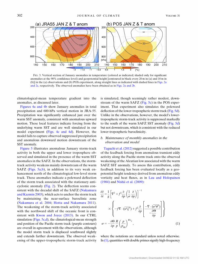
Figures 4a and 4b show January anomalies in total

precipitation and 600-hPa vertical motion in JRA-55.

Precipitation was significantly enhanced just over the

warm SST anomaly, consistent with anomalous upward

motion. These local features indicate forcing from the

underlying warm SST and are well simulated in our

model experiment (Figs. 4c and 4d). However, the

model fails to capture observed suppressed precipitation

and anomalous downward motion downstream of the

SST anomaly.

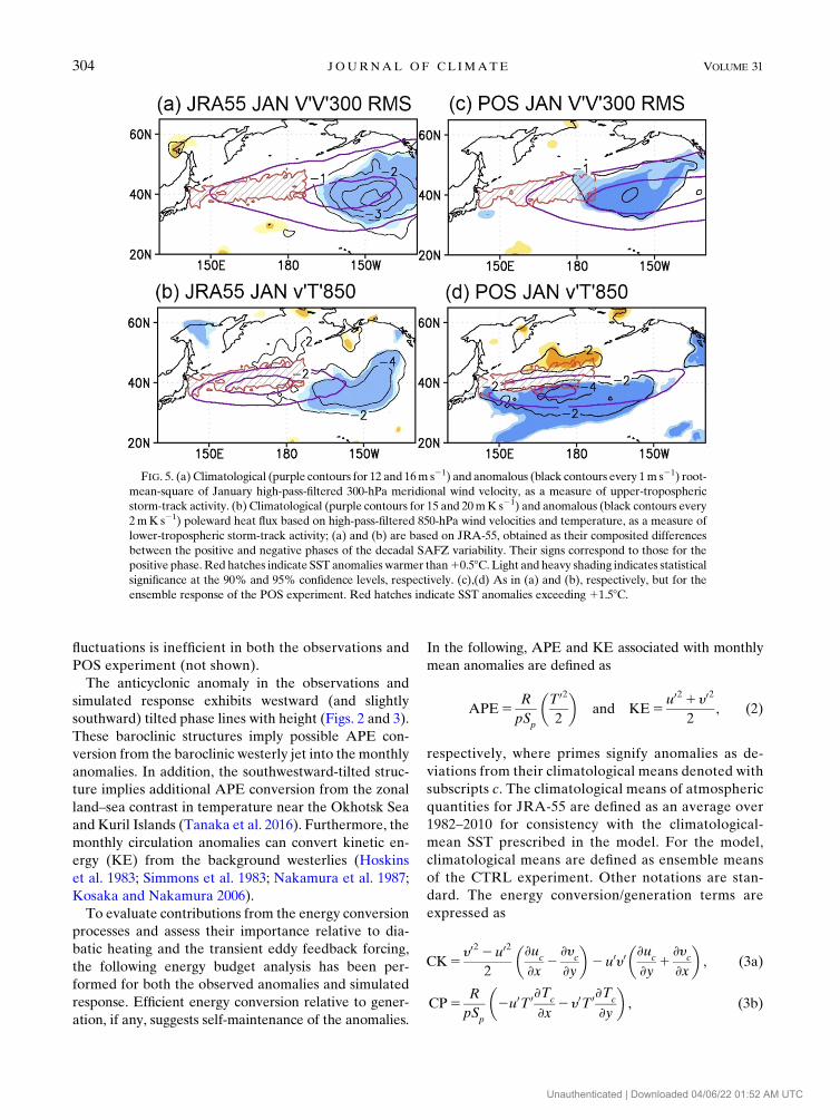
Figure 5 illustrates anomalous January storm-track

activity in both the upper and lower troposphere ob-

served and simulated in the presence of the warm SST

anomalies in the SAFZ. In the observations, the storm-

track activity weakens mainly downstream of the warm

SAFZ (Figs. 5a,b), in addition to its very weak en-

hancement north of the climatological low-level storm

track. These anomalies indicate a poleward deflection

of the storm track associated with the stationary anti-

cyclonic anomaly (Fig. 2). The deflection seems con-

sistent with the decadal shift of the SAFZ (Nakamura

andKazmin 2003), which acts to anchor the storm track

by maintaining the near-surface baroclinic zone

(Nakamura et al. 2004; Hotta and Nakamura 2011).

The weakening of the storm-track activity associated

with the northward shift of the oceanic front is con-

sistent with Kwon and Joyce (2013). In our CTRL

simulation (Figs. 5c,d), the climatological-mean strength

and position of the Pacific storm track (purple contours)

are overall in agreement with the observations, although

the model storm track is displaced southward slightly

and extends farther downstream. The observed weak-

ening of the upper-tropospheric storm-track activity

is simulated, though seemingly rather modest, down-

stream of the warm SAFZ (Fig. 5c) in the POS exper-

iment. That experiment also simulates the poleward

deflection of the lower-tropospheric storm track (Fig. 5d).

Unlike in the observations, however, the model’s lower-

tropospheric storm-track activity is suppressed markedly

to the south of the warm SAFZ SST anomaly (Fig. 5d)

but not downstream, which is consistent with the reduced

lower-tropospheric baroclinicity.

b. Maintenance of monthly anomalies in theobservation and model

Taguchi et al. (2012) suggested a possible contribution

of the feedback forcing from anomalous transient eddy

activity along the Pacific storm track onto the observed

weakening of theAleutian low associated with the warm

SAFZ SST anomaly. To assess this contribution, eddy

feedback forcing has been evaluated locally as a geo-

potential height tendency derived from anomalous eddy

vorticity and heat fluxes, as in Lau and Holopainen

(1984) and Nishii et al. (2009):

›z

›t51

g

�=2 1 f 2

›

›p

�1

s

›

›p

��21

3

8<:2f= � (y00z00)1 f 2

›

›p

2= � (y00u00)2›Q

›p

2664

3775

9=;

s52›Q

›p

R

p

�p

p00

�R/cp

, (1)

where the notations are standard unless noted otherwise.

In (1), quantitieswith double primes signify high-frequency

FIG. 3. Vertical section of January anomalies in temperature (colored as indicated; shaded only for significant

anomalies at the 90% confidence level) and geopotential height [contoured in black every 20m in (a) and 10m in

(b)] in the (a) observations and (b) POS experiment, along straight lines as indicated with dashed lines in Figs. 2a

and 2c, respectively. The observed anomalies have been obtained as in Figs. 2a and 2b.

302 JOURNAL OF CL IMATE VOLUME 31

Unauthenticated | Downloaded 04/06/22 01:52 AM UTC

fluctuations associated with transient eddies, which were

estimated locally from 6-hourly deviations from 5-day

running means. Quantities with overbars represent

monthly mean values. In addition, submonthly quasi-

stationary fluctuations whose period is longer than a

week, including blocking anomalies, can also exert

feedback forcing on monthly mean anomalies. Their

forcing was estimated from local deviations of the 5-day

runningmeans from themonthlymean fields in amanner

analogous to (1). Since those high- and low-frequency

transients keep exerting feedback forcing onto the

background state in which they are embedded, climato-

logically this feedback forcing must be compensated for

by other processes. Height tendencies have been com-

puted through (1) from the JRA-55 data and model

output, and the effective feedback forcing on monthly

anomalies is therefore evaluated from the anomalous

height tendency after removing the climatological-mean

tendency.

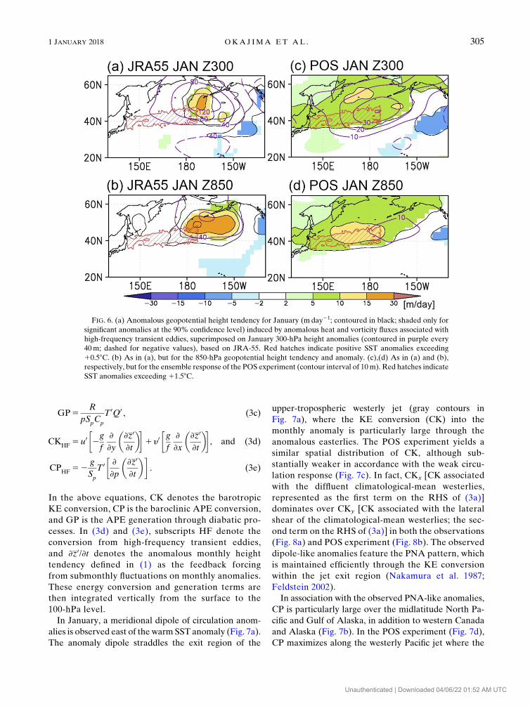
As shown in Figs. 6a and 6b, transient eddies migrat-

ing along the Pacific storm track, as the net, act to

reinforce the anticyclonic anomaly observed over the

North Pacific. The anomalous height tendency by these

feedback forcings is so efficient that it could replenish

the observed monthly anticyclonic anomaly within a

week or so in both the lower and upper troposphere. The

anomalous eddy vorticity flux acts to induce an anticy-

clonic tendency in both the upper and lower troposphere

as a positive feedback forcing. Meanwhile, the anoma-

lous eddy heat flux acts to induce anomalous cyclonic

and anticyclonic tendencies in the upper and lower

troposphere, respectively (not shown), consistent with

Lau and Nath (1991). The POS experiment captures the

observed eddy feedback forcing anomaly but in a sub-

stantially smaller magnitude (Figs. 6c and 6d). The

weaker forcing is attributable partly to the weaker

model anticyclonic response (Fig. 2). In addition, the

induced anomalous height tendency does not coincide

well with the height response, suggesting that transient

eddy feedback forcing is not quite efficient in main-

taining the simulated monthly response. Anomalous

feedback forcing from submonthly quasi-stationary

FIG. 4. January anomalies of (a) total precipitation (contoured for 60.5, 1, 2, and 3mmday21; shaded and only

for significant anomalies at the 90% confidence level) and (b) 600-hPa vertical motion (contoured for610, 20, and

30 hPa day21; colored as indicated and only for significant anomalies at the 90%confidence level) based on JRA-55.

Red hatches indicate SST anomalies exceeding10.58C. (c),(d) As in (a) and (b), respectively, but for the ensemble

response in the POS experiment. Red hatches indicate SST anomalies exceeding 11.58C.

1 JANUARY 2018 OKA J IMA ET AL . 303

Unauthenticated | Downloaded 04/06/22 01:52 AM UTC

fluctuations is inefficient in both the observations and

POS experiment (not shown).

The anticyclonic anomaly in the observations and

simulated response exhibits westward (and slightly

southward) tilted phase lines with height (Figs. 2 and 3).

These baroclinic structures imply possible APE con-

version from the baroclinic westerly jet into the monthly

anomalies. In addition, the southwestward-tilted struc-

ture implies additional APE conversion from the zonal

land–sea contrast in temperature near the Okhotsk Sea

and Kuril Islands (Tanaka et al. 2016). Furthermore, the

monthly circulation anomalies can convert kinetic en-

ergy (KE) from the background westerlies (Hoskins

et al. 1983; Simmons et al. 1983; Nakamura et al. 1987;

Kosaka and Nakamura 2006).

To evaluate contributions from the energy conversion

processes and assess their importance relative to dia-

batic heating and the transient eddy feedback forcing,

the following energy budget analysis has been per-

formed for both the observed anomalies and simulated

response. Efficient energy conversion relative to gener-

ation, if any, suggests self-maintenance of the anomalies.

In the following, APE and KE associated with monthly

mean anomalies are defined as

APE5R

pSp

�T 02

2

�and KE5

u02 1 y02

2, (2)

respectively, where primes signify anomalies as de-

viations from their climatological means denoted with

subscripts c. The climatological means of atmospheric

quantities for JRA-55 are defined as an average over

1982–2010 for consistency with the climatological-

mean SST prescribed in the model. For the model,

climatological means are defined as ensemble means

of the CTRL experiment. Other notations are stan-

dard. The energy conversion/generation terms are

expressed as

CK5y02 2 u02

2

�›u

c

›x2

›yc

›y

�2 u0y0

�›u

c

›y1

›yc

›x

�, (3a)

CP5R

pSp

�2u0T 0›Tc

›x2 y0T 0›Tc

›y

�, (3b)

FIG. 5. (a) Climatological (purple contours for 12 and 16m s21) and anomalous (black contours every 1m s21) root-

mean-square of January high-pass-filtered 300-hPa meridional wind velocity, as a measure of upper-tropospheric

storm-track activity. (b) Climatological (purple contours for 15 and 20mK s21) and anomalous (black contours every

2mK s21) poleward heat flux based on high-pass-filtered 850-hPa wind velocities and temperature, as a measure of

lower-tropospheric storm-track activity; (a) and (b) are based on JRA-55, obtained as their composited differences

between the positive and negative phases of the decadal SAFZ variability. Their signs correspond to those for the

positive phase.Red hatches indicate SST anomalies warmer than10.58C.Light and heavy shading indicates statisticalsignificance at the 90% and 95% confidence levels, respectively. (c),(d) As in (a) and (b), respectively, but for the

ensemble response of the POS experiment. Red hatches indicate SST anomalies exceeding 11.58C.

304 JOURNAL OF CL IMATE VOLUME 31

Unauthenticated | Downloaded 04/06/22 01:52 AM UTC

GP5R

pSpC

p

T 0Q0 , (3c)

CKHF

5 u0�2g

f

›

›y

�›z0

›t

��1 y0

�g

f

›

›x

�›z0

›t

��, and (3d)

CPHF

52g

Sp

T 0�›

›p

�›z0

›t

��. (3e)

In the above equations, CK denotes the barotropic

KE conversion, CP is the baroclinic APE conversion,

and GP is the APE generation through diabatic pro-

cesses. In (3d) and (3e), subscripts HF denote the

conversion from high-frequency transient eddies,

and ›z0/›t denotes the anomalous monthly height

tendency defined in (1) as the feedback forcing

from submonthly fluctuations on monthly anomalies.

These energy conversion and generation terms are

then integrated vertically from the surface to the

100-hPa level.

In January, a meridional dipole of circulation anom-

alies is observed east of the warm SST anomaly (Fig. 7a).

The anomaly dipole straddles the exit region of the

upper-tropospheric westerly jet (gray contours in

Fig. 7a), where the KE conversion (CK) into the

monthly anomaly is particularly large through the

anomalous easterlies. The POS experiment yields a

similar spatial distribution of CK, although sub-

stantially weaker in accordance with the weak circu-

lation response (Fig. 7c). In fact, CKx [CK associated

with the diffluent climatological-mean westerlies,

represented as the first term on the RHS of (3a)]

dominates over CKy [CK associated with the lateral

shear of the climatological-mean westerlies; the sec-

ond term on the RHS of (3a)] in both the observations

(Fig. 8a) and POS experiment (Fig. 8b). The observed

dipole-like anomalies feature the PNA pattern, which

is maintained efficiently through the KE conversion

within the jet exit region (Nakamura et al. 1987;

Feldstein 2002).

In association with the observed PNA-like anomalies,

CP is particularly large over the midlatitude North Pa-

cific and Gulf of Alaska, in addition to western Canada

and Alaska (Fig. 7b). In the POS experiment (Fig. 7d),

CP maximizes along the westerly Pacific jet where the

FIG. 6. (a) Anomalous geopotential height tendency for January (m day21; contoured in black; shaded only for

significant anomalies at the 90% confidence level) induced by anomalous heat and vorticity fluxes associated with

high-frequency transient eddies, superimposed on January 300-hPa height anomalies (contoured in purple every

40m; dashed for negative values), based on JRA-55. Red hatches indicate positive SST anomalies exceeding

10.58C. (b) As in (a), but for the 850-hPa geopotential height tendency and anomaly. (c),(d) As in (a) and (b),

respectively, but for the ensemble response of the POS experiment (contour interval of 10m). Red hatches indicate

SST anomalies exceeding 11.58C.

1 JANUARY 2018 OKA J IMA ET AL . 305

Unauthenticated | Downloaded 04/06/22 01:52 AM UTC

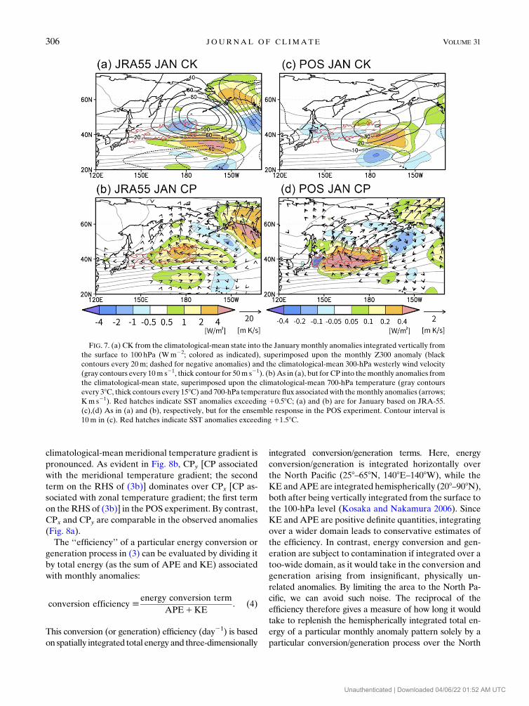
climatological-mean meridional temperature gradient is

pronounced. As evident in Fig. 8b, CPy [CP associated

with the meridional temperature gradient; the second

term on the RHS of (3b)] dominates over CPx [CP as-

sociated with zonal temperature gradient; the first term

on the RHS of (3b)] in the POS experiment. By contrast,

CPx and CPy are comparable in the observed anomalies

(Fig. 8a).

The ‘‘efficiency’’ of a particular energy conversion or

generation process in (3) can be evaluated by dividing it

by total energy (as the sum of APE and KE) associated

with monthly anomalies:

conversion efficiency [energy conversion term

APE1KE. (4)

This conversion (or generation) efficiency (day21) is based

on spatially integrated total energy and three-dimensionally

integrated conversion/generation terms. Here, energy

conversion/generation is integrated horizontally over

the North Pacific (258–658N, 1408E–1408W), while the

KE andAPE are integrated hemispherically (208–908N),

both after being vertically integrated from the surface to

the 100-hPa level (Kosaka and Nakamura 2006). Since

KE andAPE are positive definite quantities, integrating

over a wider domain leads to conservative estimates of

the efficiency. In contrast, energy conversion and gen-

eration are subject to contamination if integrated over a

too-wide domain, as it would take in the conversion and

generation arising from insignificant, physically un-

related anomalies. By limiting the area to the North Pa-

cific, we can avoid such noise. The reciprocal of the

efficiency therefore gives a measure of how long it would

take to replenish the hemispherically integrated total en-

ergy of a particular monthly anomaly pattern solely by a

particular conversion/generation process over the North

FIG. 7. (a) CK from the climatological-mean state into the January monthly anomalies integrated vertically from

the surface to 100 hPa (Wm22; colored as indicated), superimposed upon the monthly Z300 anomaly (black

contours every 20m; dashed for negative anomalies) and the climatological-mean 300-hPa westerly wind velocity

(gray contours every 10m s21, thick contour for 50m s21). (b)As in (a), but for CP into themonthly anomalies from

the climatological-mean state, superimposed upon the climatological-mean 700-hPa temperature (gray contours

every 38C, thick contours every 158C) and 700-hPa temperature flux associated with themonthly anomalies (arrows;

Km s21). Red hatches indicate SST anomalies exceeding 10.58C; (a) and (b) are for January based on JRA-55.

(c),(d) As in (a) and (b), respectively, but for the ensemble response in the POS experiment. Contour interval is

10m in (c). Red hatches indicate SST anomalies exceeding 11.58C.

306 JOURNAL OF CL IMATE VOLUME 31

Unauthenticated | Downloaded 04/06/22 01:52 AM UTC

Pacific. Table 1 summarizes the efficiency thus evaluated

for each of conversion and generation processes.

For the anomalies observed in January, contributions

from CK, CP, and the net transient eddy forcing (TE in

Table 1) based on the JRA-55 data are important for the

maintenance of the monthly anomalies, consistent with

the aforementioned height tendency analysis. In par-

ticular, CK and CP are so efficient that they can re-

plenish the total energy over the Northern Hemisphere

only in 10 days or so. The net contribution from the

feedback forcing by transient eddies along the storm

track is positive but to a lesser degree, as it can replenish

the hemispheric energy nearly in a month. This positive

contribution is through efficient barotropic feedback

forcing from transient eddies. Diabatic processes (GP),

including longwave radiation, act to damp the observed

thermal anomalies.

In the POS experiment, CP is the most efficient pro-

cess for the maintenance of the response in January,

whose conversion efficiency is about 0.08 day21 (Table

1), while CK is less efficient. The particularly efficient

CP in the model seems consistent with the well-defined

baroclinic structure of the anticyclonic response, whose

westward-tilting structure seems more apparent than in

the observed anomalies (Fig. 3). The maintenance

through TE is as efficient as in the observations. These

results indicate that the energy conversion from the

background state ismost efficient for themaintenance of

the observed anomaly pattern and model response. This

is suggestive of their characteristics as a ‘‘dynamical

mode’’ (Kosaka and Nakamura 2006, 2010), which is

inherent to the climatological-mean state of the westerly

jet, planetary waves, and associated background thermal

gradient. Among the energy conversion/generation

terms, the most distinct difference between the obser-

vations and themodel appears in GP (energy generation

through diabatic heating). For the observed anomalies

GP as the net is negative and acts as a damping, while

positive GP in the model indicates efficient forcing to

the response. This discrepancy arises mainly from dif-

ferences in the anomalous turbulent heat flux and pre-

cipitation. As shown in Fig. 9a, the anomalous surface

turbulent heat flux based on the JRA-55 data is nearly

zero over the warm SST anomaly andweakly negative to

the east. The diminished anomalous surface heat flux

indicates cancelation between anomalous upward heat

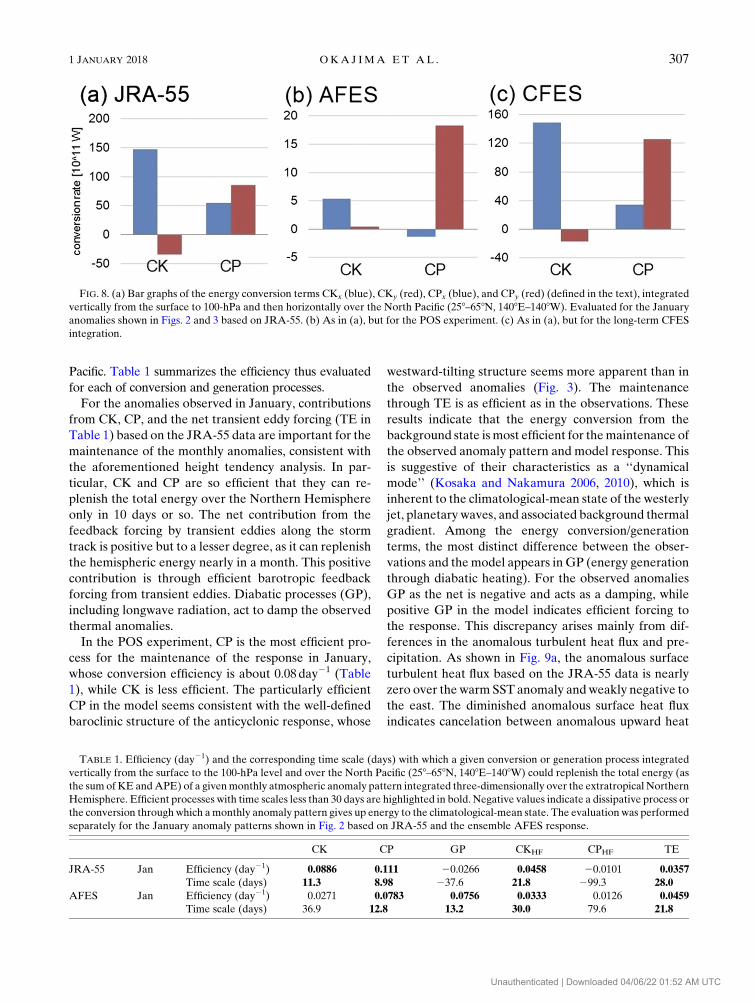
FIG. 8. (a) Bar graphs of the energy conversion terms CKx (blue), CKy (red), CPx (blue), and CPy (red) (defined in the text), integrated

vertically from the surface to 100-hPa and then horizontally over the North Pacific (258–658N, 1408E–1408W). Evaluated for the January

anomalies shown in Figs. 2 and 3 based on JRA-55. (b) As in (a), but for the POS experiment. (c) As in (a), but for the long-term CFES

integration.

TABLE 1. Efficiency (day21) and the corresponding time scale (days) with which a given conversion or generation process integrated

vertically from the surface to the 100-hPa level and over the North Pacific (258–658N, 1408E–1408W) could replenish the total energy (as

the sum of KE andAPE) of a givenmonthly atmospheric anomaly pattern integrated three-dimensionally over the extratropical Northern

Hemisphere. Efficient processes with time scales less than 30 days are highlighted in bold. Negative values indicate a dissipative process or

the conversion throughwhich amonthly anomaly pattern gives up energy to the climatological-mean state. The evaluation was performed

separately for the January anomaly patterns shown in Fig. 2 based on JRA-55 and the ensemble AFES response.

CK CP GP CKHF CPHF TE

JRA-55 Jan Efficiency (day21) 0.0886 0.111 20.0266 0.0458 20.0101 0.0357

Time scale (days) 11.3 8.98 237.6 21.8 299.3 28.0

AFES Jan Efficiency (day21) 0.0271 0.0783 0.0756 0.0333 0.0126 0.0459Time scale (days) 36.9 12.8 13.2 30.0 79.6 21.8

1 JANUARY 2018 OKA J IMA ET AL . 307

Unauthenticated | Downloaded 04/06/22 01:52 AM UTC

flux tendency due to the local warm SST anomaly and an

offsetting contribution from the anomalous surface

easterlies associated with the anticyclonic anomalies

(Fig. 2b) that act to suppress the heat/moisture release.

In the POS experiment, by contrast, the surface anticy-

clonic response and associated anomalous surface east-

erlies are quite weak (Fig. 2d), leading to enhanced heat

release from the (inflated) SST anomaly prescribed

(Fig. 9b). As evident in Fig. 4c, the strong positive pre-

cipitation response is confined into the region over the

prescribed SST anomaly, where the lower and mid-

troposphere are anomalously warm (Fig. 3b). These

discrepancies are likely attributable to the different

causality between the observations and AGCM experi-

ment (cf. Sutton and Mathieu 2002). In the POS ex-

periment, by design, GP should be positive since the

SAFZ SST anomaly is the cause of the atmospheric re-

sponse via thermal forcing. In the observations, by

contrast, the SST anomalies (including the warm

anomaly around the SAFZ) are a mixture of forcing on,

and response to, the atmospheric anomalies, and

anomalous surface heat fluxes cannot necessarily be

determined by the SST anomalies.

Maintenance mechanisms for the atmospheric anom-

alies associated with the decadal-scale SAFZ variability

in the long-term CGCM integration analyzed by Taguchi

et al. (2012) are also examined by applying the same

analysis as above. Here, atmospheric anomalies have

been extracted in the same manner as for JRA-55.

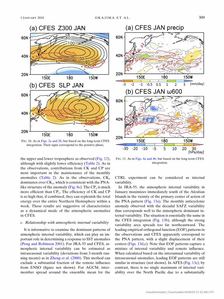
Figure 10 shows January anomalies of Z300 and SLP

thus extracted from the positive and negative phases

(26–30 and 56–60model years, respectively) of the

model SAFZ variability. The equivalent barotropic

anticyclonic anomaly is in good agreement with the

corresponding signal in Taguchi et al. (2012, their

Figs. 10b and 10c). The pattern in the CFES simulation

resembles the observed pattern more than the AFES

response. Enhanced precipitation and anomalous up-

ward motion over the warm SST anomaly is also consis-

tent with the observations and POS experiment (Fig. 11).

The anomalous turbulent heat flux is similar to the

observational counterpart, except for larger upward heat

flux anomaly in the western part of the SST anomaly due

probably to the larger SST anomaly in CFES (28–38C;Taguchi et al. 2012) than in the observations (Fig. 9c).

Table 2 summarizes the same energetic analysis as above

applied to the monthly anomalies in CFES, and GP is

missing owing to the lack of diabatic heating data in the

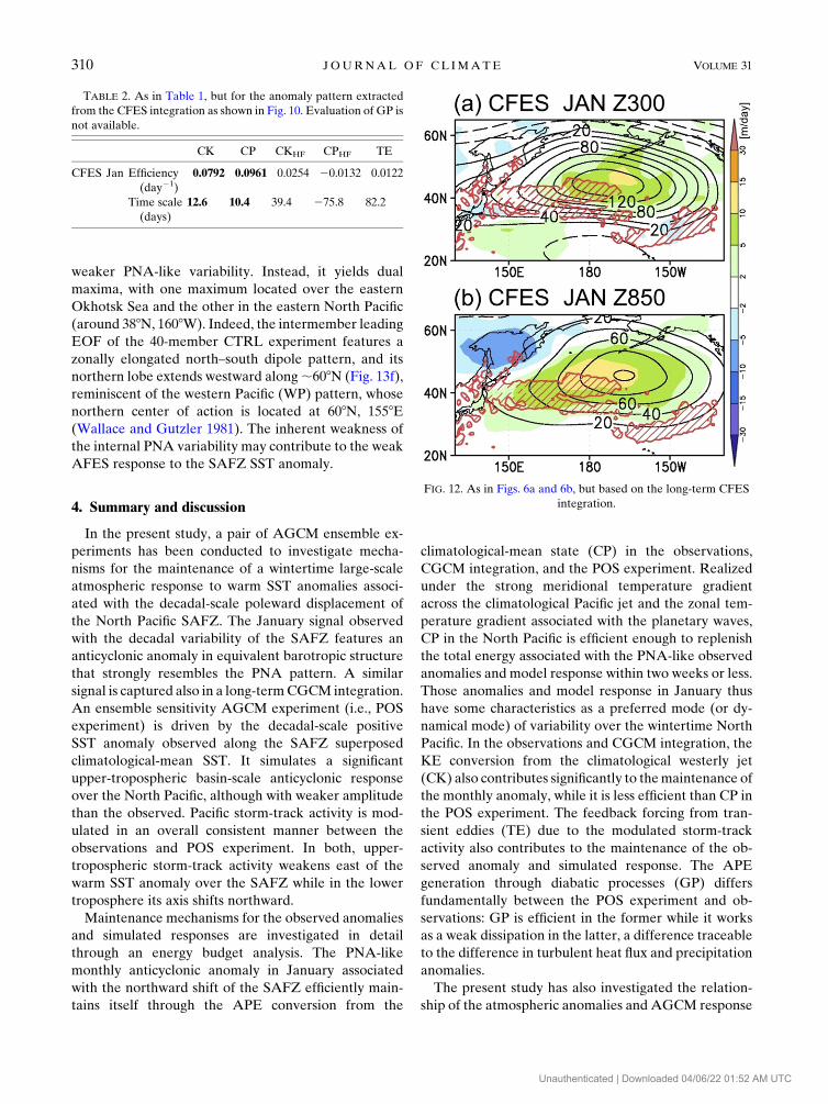
model output. The transient eddy feedback forcing acts to

reinforce themonthlymean anticyclonic anomaly in both

FIG. 9. (a) January anomalies of the net surface turbulent heat flux (colored as indicated) based on JRA-55.

Positive values indicate heat released from the ocean. (b) As in (a), but for the ensemble response in the POS

experiment. (c) As in (a), but based on the long-term CFES integration. Red hatches indicate positive SST

anomalies exceeding 10.58C in (a) and (c) and 11.58C in (b).

308 JOURNAL OF CL IMATE VOLUME 31

Unauthenticated | Downloaded 04/06/22 01:52 AM UTC

the upper and lower troposphere as observed (Fig. 12),

although with slightly lower efficiency (Table 2). As in

the observations, contributions from CK and CP are

most important in the maintenance of the monthly

anomalies (Table 2). As in the observations, CKx

dominates over CKy, which is consistent with the PNA-

like structure of the anomaly (Fig. 8c). The CPy is much

more efficient than CPx. The efficiency of CK and CP

is so high that, if combined, they can replenish the total

energy over the entire Northern Hemisphere within a

week. These results are suggestive of characteristics

as a dynamical mode of the atmospheric anomalies

in CFES.

c. Relationship with atmospheric internal variability

It is informative to examine the dominant patterns of

atmospheric internal variability, which can play an im-

portant role in determining a response to SST anomalies

(Peng and Robinson 2001). For JRA-55 and CFES, at-

mospheric internal variability can be estimated as

intraseasonal variability (deviations from 3-month run-

ning means) as in Zheng et al. (2000). This method can

exclude a substantial fraction of the remote influence

from ENSO (figure not shown). For AGCM, inter-

member spread around the ensemble mean for the

CTRL experiment can be considered as internal

variability.

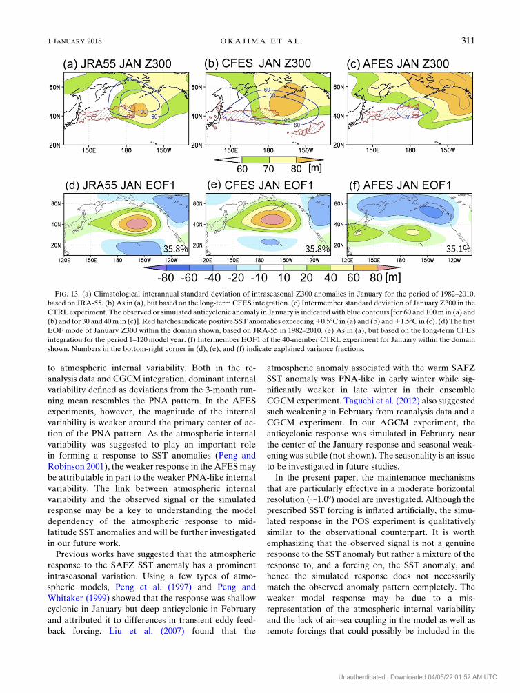
In JRA-55, the atmospheric internal variability in

January maximizes immediately south of the Aleutian

Islands in the vicinity of the primary center of action of

the PNA pattern (Fig. 13a). The monthly anticyclonic

anomaly observed with the decadal SAFZ variability

thus corresponds well to the atmospheric dominant in-

ternal variability. The situation is essentially the same in

the CFES integration (Fig. 13b), although the strong

variability area spreads too far northeastward. The

leading empirical orthogonal function (EOF) patterns in

the observations and CFES apparently correspond to

the PNA pattern, with a slight displacement of their

centers (Figs. 13d,e). Note that EOF patterns capture a

mixture of internal variability and remote influence.

When calculated based on the interannual variability of

intraseasonal anomalies, leading EOF patterns are still

similar in structure (not shown). In AFES (Fig. 13c), by

contrast, there is no single maximum of internal vari-

ability over the North Pacific due to a substantially

FIG. 10. As in Figs. 2a and 2b, but based on the long-term CFES

integration. Their signs correspond to the positive phase.

FIG. 11. As in Figs. 4a and 4b, but based on the long-term CFES

integration.

1 JANUARY 2018 OKA J IMA ET AL . 309

Unauthenticated | Downloaded 04/06/22 01:52 AM UTC

weaker PNA-like variability. Instead, it yields dual

maxima, with one maximum located over the eastern

Okhotsk Sea and the other in the eastern North Pacific

(around 388N, 1608W). Indeed, the intermember leading

EOF of the 40-member CTRL experiment features a

zonally elongated north–south dipole pattern, and its

northern lobe extends westward along;608N (Fig. 13f),

reminiscent of the western Pacific (WP) pattern, whose

northern center of action is located at 608N, 1558E(Wallace and Gutzler 1981). The inherent weakness of

the internal PNA variability may contribute to the weak

AFES response to the SAFZ SST anomaly.

4. Summary and discussion

In the present study, a pair of AGCM ensemble ex-

periments has been conducted to investigate mecha-

nisms for the maintenance of a wintertime large-scale

atmospheric response to warm SST anomalies associ-

ated with the decadal-scale poleward displacement of

the North Pacific SAFZ. The January signal observed

with the decadal variability of the SAFZ features an

anticyclonic anomaly in equivalent barotropic structure

that strongly resembles the PNA pattern. A similar

signal is captured also in a long-termCGCM integration.

An ensemble sensitivity AGCM experiment (i.e., POS

experiment) is driven by the decadal-scale positive

SST anomaly observed along the SAFZ superposed

climatological-mean SST. It simulates a significant

upper-tropospheric basin-scale anticyclonic response

over the North Pacific, although with weaker amplitude

than the observed. Pacific storm-track activity is mod-

ulated in an overall consistent manner between the

observations and POS experiment. In both, upper-

tropospheric storm-track activity weakens east of the

warm SST anomaly over the SAFZ while in the lower

troposphere its axis shifts northward.

Maintenance mechanisms for the observed anomalies

and simulated responses are investigated in detail

through an energy budget analysis. The PNA-like

monthly anticyclonic anomaly in January associated

with the northward shift of the SAFZ efficiently main-

tains itself through the APE conversion from the

climatological-mean state (CP) in the observations,

CGCM integration, and the POS experiment. Realized

under the strong meridional temperature gradient

across the climatological Pacific jet and the zonal tem-

perature gradient associated with the planetary waves,

CP in the North Pacific is efficient enough to replenish

the total energy associated with the PNA-like observed

anomalies and model response within two weeks or less.

Those anomalies and model response in January thus

have some characteristics as a preferred mode (or dy-

namical mode) of variability over the wintertime North

Pacific. In the observations and CGCM integration, the

KE conversion from the climatological westerly jet

(CK) also contributes significantly to themaintenance of

the monthly anomaly, while it is less efficient than CP in

the POS experiment. The feedback forcing from tran-

sient eddies (TE) due to the modulated storm-track

activity also contributes to the maintenance of the ob-

served anomaly and simulated response. The APE

generation through diabatic processes (GP) differs

fundamentally between the POS experiment and ob-

servations: GP is efficient in the former while it works

as a weak dissipation in the latter, a difference traceable

to the difference in turbulent heat flux and precipitation

anomalies.

The present study has also investigated the relation-

ship of the atmospheric anomalies and AGCM response

TABLE 2. As in Table 1, but for the anomaly pattern extracted

from the CFES integration as shown in Fig. 10. Evaluation of GP is

not available.

CK CP CKHF CPHF TE

CFES Jan Efficiency

(day21)

0.0792 0.0961 0.0254 20.0132 0.0122

Time scale

(days)

12.6 10.4 39.4 275.8 82.2

FIG. 12. As in Figs. 6a and 6b, but based on the long-term CFES

integration.

310 JOURNAL OF CL IMATE VOLUME 31

Unauthenticated | Downloaded 04/06/22 01:52 AM UTC

to atmospheric internal variability. Both in the re-

analysis data and CGCM integration, dominant internal

variability defined as deviations from the 3-month run-

ning mean resembles the PNA pattern. In the AFES

experiments, however, the magnitude of the internal

variability is weaker around the primary center of ac-

tion of the PNA pattern. As the atmospheric internal

variability was suggested to play an important role

in forming a response to SST anomalies (Peng and

Robinson 2001), the weaker response in the AFESmay

be attributable in part to the weaker PNA-like internal

variability. The link between atmospheric internal

variability and the observed signal or the simulated

response may be a key to understanding the model

dependency of the atmospheric response to mid-

latitude SST anomalies and will be further investigated

in our future work.

Previous works have suggested that the atmospheric

response to the SAFZ SST anomaly has a prominent

intraseasonal variation. Using a few types of atmo-

spheric models, Peng et al. (1997) and Peng and

Whitaker (1999) showed that the response was shallow

cyclonic in January but deep anticyclonic in February

and attributed it to differences in transient eddy feed-

back forcing. Liu et al. (2007) found that the

atmospheric anomaly associated with the warm SAFZ

SST anomaly was PNA-like in early winter while sig-

nificantly weaker in late winter in their ensemble

CGCM experiment. Taguchi et al. (2012) also suggested

such weakening in February from reanalysis data and a

CGCM experiment. In our AGCM experiment, the

anticyclonic response was simulated in February near

the center of the January response and seasonal weak-

ening was subtle (not shown). The seasonality is an issue

to be investigated in future studies.

In the present paper, the maintenance mechanisms

that are particularly effective in a moderate horizontal

resolution (;1.08) model are investigated. Although the

prescribed SST forcing is inflated artificially, the simu-

lated response in the POS experiment is qualitatively

similar to the observational counterpart. It is worth

emphasizing that the observed signal is not a genuine

response to the SST anomaly but rather a mixture of the

response to, and a forcing on, the SST anomaly, and

hence the simulated response does not necessarily

match the observed anomaly pattern completely. The

weaker model response may be due to a mis-

representation of the atmospheric internal variability

and the lack of air–sea coupling in the model as well as

remote forcings that could possibly be included in the

FIG. 13. (a) Climatological interannual standard deviation of intraseasonal Z300 anomalies in January for the period of 1982–2010,

based on JRA-55. (b) As in (a), but based on the long-termCFES integration. (c) Intermember standard deviation of January Z300 in the

CTRL experiment. The observed or simulated anticyclonic anomaly in January is indicated with blue contours [for 60 and 100m in (a) and

(b) and for 30 and 40m in (c)]. Red hatches indicate positive SST anomalies exceeding10.58C in (a) and (b) and11.58C in (c). (d) The first

EOF mode of January Z300 within the domain shown, based on JRA-55 in 1982–2010. (e) As in (a), but based on the long-term CFES

integration for the period 1–120model year. (f) Intermember EOF1 of the 40-member CTRL experiment for January within the domain

shown. Numbers in the bottom-right corner in (d), (e), and (f) indicate explained variance fractions.

1 JANUARY 2018 OKA J IMA ET AL . 311

Unauthenticated | Downloaded 04/06/22 01:52 AM UTC

observations. In our AGCMwith;1.08 3 1.08 horizontalresolution, the most effective maintenance mechanism is

energy conversion from the climatological background

state along with efficient transient feedback forcing, and

diabatic processes are also important. This implies that a

moderate-resolution (;1.08) AGCM is able to simulate a

basin-scale atmospheric response to the SAFZ SST

anomaly through synoptic- and basin-scale dynamical

processes, a complementary view to the study by Smirnov

et al. (2015), who found that a robust anticyclonic re-

sponse with realistic strength was simulated only in their

higher-resolution (0.258 3 0.258) AGCM against a warm

SST anomaly in the SAFZ with realistic strength. They

claimed that diabatic processes associated with cumulus

convection that can be better represented in their high-

resolution model are critical for the robust basin-scale

atmospheric response. Interestingly, our AGCM re-

sponse is anticyclonic to the east of the warm SST

anomaly, which is qualitatively similar to their higher-

resolution AGCM result, although the prescribed SST

anomaly needs to be inflated in the present study to

obtain a robust response. The weak amplitude in our

AGCM response is presumably related to its insufficient

ability to represent mesoscale precipitation systems and

the lack of daily variability in the background SST (Zhou

et al. 2015, 2017). The former can be important for effi-

ciently triggering a robust basin-scale response to a warm

SST anomaly in the SAFZ by sensitively modulating the

Pacific storm-track activity. Resolution dependence of

the model atmospheric response to the SAFZ variability

will be investigated in future study.

Acknowledgments.The authors thank Justin Small for

giving us valuable comments. We also thank two anon-

ymous reviewers for their useful and constructive com-

ments that have led our paper to its substantial

improvement. This study is supported in part by the

Japanese Ministry of Education, Culture, Sports, Science

and Technology (MEXT) through a Grant-in-Aid for

Scientific Research in Innovative Area 2205 and through

the Arctic Challenge for Sustainability (ArCS) Program

and by the Japanese Ministry of Environment through

the Environment Research and Technology Department

Fund 2-1503. This work was also supported by the Japan

Society for the Promotion of Science (JSPS) through

KAKENHI Grants 15J04846 for JSPS Research Fellows

and 16H01844 and by the Japan Science and Technology

Agency through Belmont ForumCRA ‘‘InterDec.’’ S. O.

is also supported by MEXT through the Program for

Leading Graduate Schools. The Earth Simulator was

utilized in support of JAMSTEC. The JRA-55 reanalysis

dataset is provided by JMA. NOAA Optimum In-

terpolation SST data (OISST) are provided by the

NOAA-CIRES Climate Diagnostics Center, Boulder,

Colorado, from their website (http://www.cdc.noaa.gov/).

The Grid Analysis and Display System (GrADS) was

used for drawing figures.

APPENDIX

Evaluation of Remote Influence

The observed signal (shown, e.g., in Fig. 2) can be in

part influenced by remote forcing, including ENSO.

However, it is difficult to obtain SST fields in the tropics

with high reliability from the gridded ICOADS data

used in this study for the period around 1970, when the

negative phase of the decadal SAFZ variability was

observed. Instead, the Centennial In Situ Observation-

Based Estimates of SSTs (COBE-SST; Ishii et al. 2005)

and ERSST.v3b (Smith et al. 2008) are utilized. It is

found that these two datasets yield very similar results.

In the following, the statistics based on COBE-SST are

presented, which was prescribed as the boundary con-

dition for the JRA-55 reanalysis used in this study. The

following results are based on simultaneous correlation/

regression, but similar results are obtained when a one

or two month lag (ocean leads atmosphere) is taken.

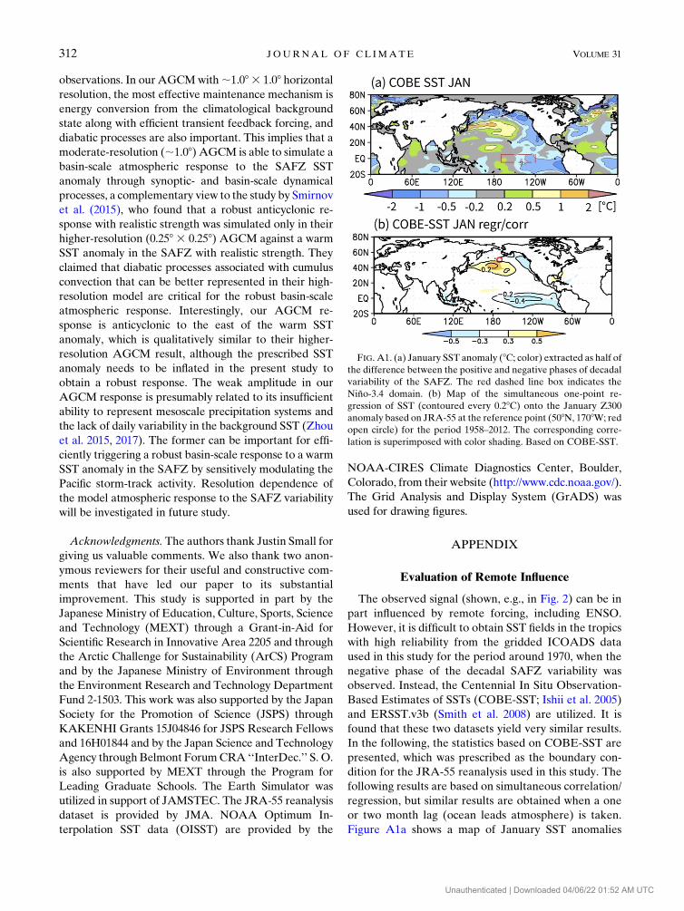
Figure A1a shows a map of January SST anomalies

FIG. A1. (a) January SST anomaly (8C; color) extracted as half ofthe difference between the positive and negative phases of decadal

variability of the SAFZ. The red dashed line box indicates the

Niño-3.4 domain. (b) Map of the simultaneous one-point re-

gression of SST (contoured every 0.28C) onto the January Z300

anomaly based on JRA-55 at the reference point (508N, 1708W; red

open circle) for the period 1958–2012. The corresponding corre-

lation is superimposed with color shading. Based on COBE-SST.

312 JOURNAL OF CL IMATE VOLUME 31

Unauthenticated | Downloaded 04/06/22 01:52 AM UTC

based on COBE-SST at a 18 horizontal resolution, whichhas been obtained as half of the difference between the

positive and negative phases of decadal variability of the

SAFZ. Defined in the same manner, Fig. A1a offers a

quasi-global view of the SST anomalies shown in Fig. 1c.

The warm SST anomaly along the North Pacific SAFZ

tends to be observed concomitantly in a weak La Niña–like situation, which potentially affects the atmospheric

anomalies shown in Fig. 2 remotely.

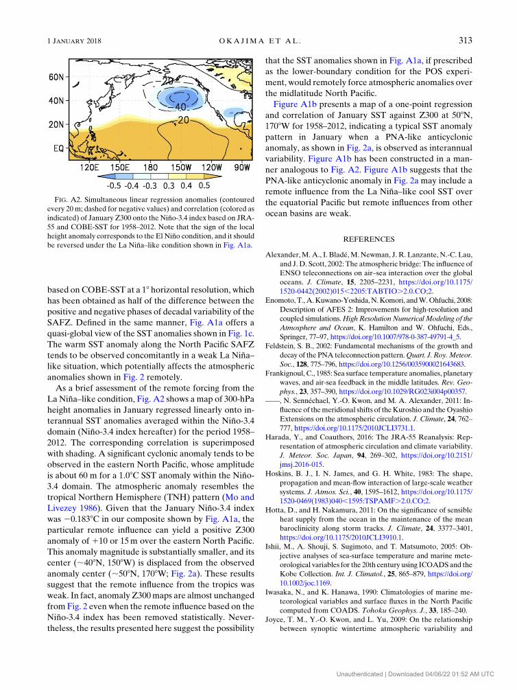
As a brief assessment of the remote forcing from the

La Niña–like condition, Fig. A2 shows a map of 300-hPa

height anomalies in January regressed linearly onto in-

terannual SST anomalies averaged within the Niño-3.4domain (Niño-3.4 index hereafter) for the period 1958–

2012. The corresponding correlation is superimposed

with shading. A significant cyclonic anomaly tends to be

observed in the eastern North Pacific, whose amplitude

is about 60 m for a 1.08C SST anomaly within the Niño-3.4 domain. The atmospheric anomaly resembles the

tropical Northern Hemisphere (TNH) pattern (Mo and

Livezey 1986). Given that the January Niño-3.4 index

was 20.1838C in our composite shown by Fig. A1a, the

particular remote influence can yield a positive Z300

anomaly of 110 or 15m over the eastern North Pacific.

This anomaly magnitude is substantially smaller, and its

center (;408N, 1508W) is displaced from the observed

anomaly center (;508N, 1708W; Fig. 2a). These results

suggest that the remote influence from the tropics was

weak. In fact, anomaly Z300maps are almost unchanged

from Fig. 2 even when the remote influence based on the

Niño-3.4 index has been removed statistically. Never-

theless, the results presented here suggest the possibility

that the SST anomalies shown in Fig. A1a, if prescribed

as the lower-boundary condition for the POS experi-

ment, would remotely force atmospheric anomalies over

the midlatitude North Pacific.

Figure A1b presents a map of a one-point regression

and correlation of January SST against Z300 at 508N,

1708W for 1958–2012, indicating a typical SST anomaly

pattern in January when a PNA-like anticyclonic

anomaly, as shown in Fig. 2a, is observed as interannual

variability. Figure A1b has been constructed in a man-

ner analogous to Fig. A2. Figure A1b suggests that the

PNA-like anticyclonic anomaly in Fig. 2a may include a

remote influence from the La Niña–like cool SST over

the equatorial Pacific but remote influences from other

ocean basins are weak.

REFERENCES

Alexander,M.A., I. Bladé, M. Newman, J. R. Lanzante, N.-C. Lau,

and J. D. Scott, 2002: The atmospheric bridge: The influence of

ENSO teleconnections on air–sea interaction over the global

oceans. J. Climate, 15, 2205–2231, https://doi.org/10.1175/

1520-0442(2002)015,2205:TABTIO.2.0.CO;2.

Enomoto, T.,A.Kuwano-Yoshida,N.Komori, andW.Ohfuchi, 2008:

Description of AFES 2: Improvements for high-resolution and

coupled simulations.HighResolutionNumericalModeling of the

Atmosphere and Ocean, K. Hamilton and W. Ohfuchi, Eds.,

Springer, 77–97, https://doi.org/10.1007/978-0-387-49791-4_5.

Feldstein, S. B., 2002: Fundamental mechanisms of the growth and

decay of thePNA teleconnection pattern.Quart. J. Roy.Meteor.

Soc., 128, 775–796, https://doi.org/10.1256/0035900021643683.

Frankignoul, C., 1985: Sea surface temperature anomalies, planetary

waves, and air-sea feedback in the middle latitudes. Rev. Geo-

phys., 23, 357–390, https://doi.org/10.1029/RG023i004p00357.

——, N. Sennéchael, Y.-O. Kwon, and M. A. Alexander, 2011: In-

fluence of themeridional shifts of theKuroshio and theOyashio

Extensions on the atmospheric circulation. J. Climate, 24, 762–

777, https://doi.org/10.1175/2010JCLI3731.1.

Harada, Y., and Coauthors, 2016: The JRA-55 Reanalysis: Rep-

resentation of atmospheric circulation and climate variability.

J. Meteor. Soc. Japan, 94, 269–302, https://doi.org/10.2151/

jmsj.2016-015.

Hoskins, B. J., I. N. James, and G. H. White, 1983: The shape,

propagation and mean-flow interaction of large-scale weather

systems. J. Atmos. Sci., 40, 1595–1612, https://doi.org/10.1175/

1520-0469(1983)040,1595:TSPAMF.2.0.CO;2.

Hotta, D., and H. Nakamura, 2011: On the significance of sensible

heat supply from the ocean in the maintenance of the mean

baroclinicity along storm tracks. J. Climate, 24, 3377–3401,

https://doi.org/10.1175/2010JCLI3910.1.

Ishii, M., A. Shouji, S. Sugimoto, and T. Matsumoto, 2005: Ob-

jective analyses of sea-surface temperature and marine mete-

orological variables for the 20th century using ICOADSand the

Kobe Collection. Int. J. Climatol., 25, 865–879, https://doi.org/

10.1002/joc.1169.

Iwasaka, N., and K. Hanawa, 1990: Climatologies of marine me-

teorological variables and surface fluxes in the North Pacific

computed from COADS. Tohoku Geophys. J., 33, 185–240.

Joyce, T. M., Y.-O. Kwon, and L. Yu, 2009: On the relationship

between synoptic wintertime atmospheric variability and

FIG. A2. Simultaneous linear regression anomalies (contoured

every 20 m; dashed for negative values) and correlation (colored as

indicated) of January Z300 onto the Niño-3.4 index based on JRA-

55 and COBE-SST for 1958–2012. Note that the sign of the local

height anomaly corresponds to the El Niño condition, and it should

be reversed under the La Niña–like condition shown in Fig. A1a.

1 JANUARY 2018 OKA J IMA ET AL . 313

Unauthenticated | Downloaded 04/06/22 01:52 AM UTC

path shifts in the Gulf Stream and the Kuroshio Exten-

sion. J. Climate, 22, 3177–3192, https://doi.org/10.1175/

2008JCLI2690.1.

Kelly, K. A., R. J. Small, R. M. Samelson, B. Qiu, T. M. Joyce, Y.-O.

Kwon, and M. F. Cronin, 2010: Western boundary currents and

frontal air–sea interaction: Gulf Stream and Kuroshio Extension.

J.Climate, 23, 5644–5667, https://doi.org/10.1175/2010JCLI3346.1.

Kida, S., and Coauthors, 2015: Oceanic fronts and jets around Ja-

pan: A review. J. Oceanogr., 71, 469–497, https://doi.org/

10.1007/s10872-015-0283-7.

Kobayashi, S., and Coauthors, 2015: The JRA-55 Reanalysis:

General specifications and basic characteristics. J. Meteor.

Soc. Japan, 93, 5–48, https://doi.org/10.2151/jmsj.2015-001.

Komori, N., K. Takahashi, K. Komine, T. Motoi, X. Zhang, and

G. Sagawa, 2005: Description of sea-ice component of Cou-

pled Ocean–Sea-Ice Model for the Earth Simulator (OIFES).

J. Earth Simul., 4, 31–45.Kosaka, Y., andH. Nakamura, 2006: Structure and dynamics of the

summertime Pacific–Japan teleconnection pattern. Quart.

J. Roy. Meteor. Soc., 132, 2009–2030, https://doi.org/10.1256/

qj.05.204.

——, and ——, 2010: Mechanisms of meridional teleconnection

observed between a summermonsoon system and a subtropical

anticyclone. Part I: The Pacific–Japan pattern. J. Climate, 23,

5085–5108, https://doi.org/10.1175/2010JCLI3413.1.

Kushnir, Y., and N.-C. Lau, 1992: The general circulation model

response to a North Pacific SST anomaly: Dependence on time

scale and pattern polarity. J. Climate, 5, 271–283, https://doi.org/

10.1175/1520-0442(1992)005,0271:TGCMRT.2.0.CO;2.

——, W. A. Robinson, I. Bladé, N. M. J. Hall, S. Peng, and

R. Sutton, 2002: Atmospheric GCM response to extratropical

SST anomalies: Synthesis and evaluation. J. Climate, 15,

2233–2256, https://doi.org/10.1175/1520-0442(2002)015,2233:

AGRTES.2.0.CO;2.

Kuwano-Yoshida, A., T. Enomoto, and W. Ohfuchi, 2010: An

improved PDF cloud scheme for climate simulations. Quart.

J. Roy. Meteor. Soc., 136, 1583–1597, https://doi.org/10.1002/

qj.660.

Kwon, Y.-O., and T. M. Joyce, 2013: Northern Hemisphere winter

atmospheric transient eddy heat fluxes and the Gulf Stream

and Kuroshio–Oyashio Extension variability. J. Climate, 26,

9839–9859, https://doi.org/10.1175/JCLI-D-12-00647.1.

——,M.A. Alexander, N. A. Bond, C. Frankignoul, H. Nakamura,

B. Qiu, and L. A. Thompson, 2010: Role of the Gulf Stream

and Kuroshio–Oyashio systems in large-scale atmosphere–

ocean interaction: A review. J. Climate, 23, 3249–3281, https://

doi.org/10.1175/2010JCLI3343.1.

Lau, N.-C., 1997: Interactions between global SST anomalies and

the midlatitude atmospheric circulation. Bull. Amer. Meteor.

Soc., 78, 21–33, https://doi.org/10.1175/1520-0477(1997)078,0021:

IBGSAA.2.0.CO;2.

——, and E. O. Holopainen, 1984: Transient eddy forcing of

the time-mean flow as identified by geopotential tenden-

cies. J. Atmos. Sci., 41, 313–328, https://doi.org/10.1175/

1520-0469(1984)041,0313:TEFOTT.2.0.CO;2.

——, andM. J. Nath, 1990:A general circulationmodel study of the

atmospheric response to extratropical SST anomalies ob-

served in 1950–79. J. Climate, 3, 965–989, https://doi.org/

10.1175/1520-0442(1990)003,0965:AGCMSO.2.0.CO;2.

——, and ——, 1991: Variability of the baroclinic and barotropic

transient eddy forcing associated with monthly changes in the

midlatitude storm tracks. J. Atmos. Sci., 48, 2589–2613, https://

doi.org/10.1175/1520-0469(1991)048,2589:VOTBAB.2.0.CO;2.

Liu, Z., Y. Liu, L. Wu, and R. Jacob, 2007: Seasonal and long-term

atmospheric responses to reemerging North Pacific Ocean

variability: A combined dynamical and statistical assessment.

J. Climate, 20, 955–980, https://doi.org/10.1175/JCLI4041.1.

Minobe, S., and A. Maeda, 2005: A 18monthly gridded sea-surface

temperature dataset compiled from ICOADS from 1850 to

2002 and Northern Hemisphere frontal variability. Int.

J. Climatol., 25, 881–894, https://doi.org/10.1002/joc.1170.Mo, K. C., and R. E. Livezey, 1986: Tropical-extratropical geo-

potential height teleconnections during the Northern Hemi-

sphere winter.Mon. Wea. Rev., 114, 2488–2515, https://doi.org/

10.1175/1520-0493(1986)114,2488:TEGHTD.2.0.CO;2.

Nakamura, H., and A. S. Kazmin, 2003: Decadal changes in the

North Pacific oceanic frontal zones as revealed in ship and

satellite observations. J. Geophys. Res., 108, 3078, https://

doi.org/10.1029/1999JC000085.

——,M. Tanaka, and J.M.Wallace, 1987: Horizontal structure and

energetics of Northern Hemisphere wintertime teleconnec-

tion patterns. J. Atmos. Sci., 44, 3377–3391, https://doi.org/

10.1175/1520-0469(1987)044,3377:HSAEON.2.0.CO;2.

——, G. Lin, and T. Yamagata, 1997: Decadal climate vari-

ability in the North Pacific during the recent decades. Bull.

Amer. Meteor. Soc., 78, 2215–2225, https://doi.org/10.1175/

1520-0477(1997)078,2215:DCVITN.2.0.CO;2.

——, T. Sampe, Y. Tanimoto, and A. Shimpo, 2004: Observed

associations among storm tracks, jet streams andmidlatitude

oceanic fronts. Earth’s Climate: The Ocean-Atmosphere

Interaction, C. Wang, S.-P. Xie, and J. A. Carton, Eds.,

Amer. Geophys. Union, 329–346, https://doi.org/10.1029/

147GM18.

——, A. Isobe, S. Minobe, H. Mitsudera, M. Nonaka, and T. Suga,

2015: ‘‘Hot spots’’ in the climate system—New developments

in the extratropical ocean–atmosphere interaction research: A

short review and an introduction. J. Oceanogr., 71, 463–467,

https://doi.org/10.1007/s10872-015-0321-5.

Newman, M., and Coauthors, 2016: The Pacific decadal oscillation,

revisited. J. Climate, 29, 4399–4427, https://doi.org/10.1175/

JCLI-D-15-0508.1.

Nishii, K., H. Nakamura, and T. Miyasaka, 2009: Modulations in

the planetary wave field induced by upward-propagating

Rossby wave packets prior to stratospheric sudden warming

events: A case-study. Quart. J. Roy. Meteor. Soc., 135, 39–52,

https://doi.org/10.1002/qj.359.

Nonaka, M., H. Nakamura, Y. Tanimoto, T. Kagimoto, and

H. Sasaki, 2006: Decadal variability in the Kuroshio–Oyashio

Extension simulated in an eddy-resolving OGCM. J. Climate,

19, 1970–1989, https://doi.org/10.1175/JCLI3793.1.

Ohfuchi, W., and Coauthors, 2004: 10-km mesh meso-scale re-

solving simulations of the global atmosphere on the Earth

Simulator—Preliminary outcomes of AFES (AGCM for the

Earth Simulator). J. Earth Simul., 1, 8–34.——, H. Sasaki, Y. Masumoto, and H. Nakamura, 2007: ‘‘Virtual’’

atmospheric and oceanic circulations in the Earth Simulator.

Bull. Amer. Meteor. Soc., 88, 861–866, https://doi.org/10.1175/

BAMS-88-6-861.

Okajima, S., H. Nakamura, K. Nishii, T. Miyasaka, and

A. Kuwano-Yoshida, 2014: Assessing the importance of

prominent warm SST anomalies over the midlatitude North

Pacific in forcing large-scale atmospheric anomalies during

2011 summer and autumn. J. Climate, 27, 3889–3903, https://

doi.org/10.1175/JCLI-D-13-00140.1.

Onogi, K., andCoauthors, 2007: The JRA-25Reanalysis. J.Meteor.

Soc. Japan, 85, 369–432, https://doi.org/10.2151/jmsj.85.369.

314 JOURNAL OF CL IMATE VOLUME 31

Unauthenticated | Downloaded 04/06/22 01:52 AM UTC

O’Reilly, C. H., and A. Czaja, 2015: The response of the Pacific

storm track and atmospheric circulation to Kuroshio Exten-

sion variability.Quart. J. Roy.Meteor. Soc., 141, 52–66, https://

doi.org/10.1002/qj.2334.

Peng, S., and J. S. Whitaker, 1999: Mechanisms determining the

atmospheric response tomidlatitude SST anomalies. J. Climate,

12, 1393–1408, https://doi.org/10.1175/1520-0442(1999)012,1393:

MDTART.2.0.CO;2.

——, and W. A. Robinson, 2001: Relationships between atmo-

spheric internal variability and the responses to an extratropical

SST anomaly. J. Climate, 14, 2943–2959, https://doi.org/10.1175/

1520-0442(2001)014,2943:RBAIVA.2.0.CO;2.

——, L. A. Mysak, J. Derome, H. Ritchie, and B. Dugas, 1995: The

differences between early and midwinter atmospheric re-

sponses to sea surface temperature anomalies in the north-

west Atlantic. J. Climate, 8, 137–157, https://doi.org/10.1175/

1520-0442(1995)008,0137:TDBEAM.2.0.CO;2.

——, W. A. Robinson, and M. P. Hoerling, 1997: The modeled

atmospheric response to midlatitude SST anomalies and its

dependence on background circulation states. J. Climate, 10,

971–987, https://doi.org/10.1175/1520-0442(1997)010,0971:

TMARTM.2.0.CO;2.

Reynolds, R. W., T. M. Smith, C. Liu, D. B. Chelton, K. S. Casey,

and M. G. Schlax, 2007: Daily high-resolution-blended ana-

lyses for sea surface temperature. J. Climate, 20, 5473–5496,

https://doi.org/10.1175/2007JCLI1824.1.

Robinson, W. A., 2000: Review of WETS—The workshop on

extra-tropical SST anomalies. Bull. Amer. Meteor. Soc.,

81, 567–577, https://doi.org/10.1175/1520-0477(2000)081,0567:

ROWTWO.2.3.CO;2.

Schneider, N., A. J. Miller, and D. W. Pierce, 2002: Anat-

omy of North Pacific decadal variability. J. Climate, 15,

586–605, https://doi.org/10.1175/1520-0442(2002)015,0586:

AONPDV.2.0.CO;2.

Seager, R., Y. Kushnir, N. H. Naik,M. A. Cane, and J. Miller, 2001:

Wind-driven shifts in the latitude of the Kuroshio–Oyashio

Extension and generation of SST anomalies on decadal

timescales. J. Climate, 14, 4249–4265, https://doi.org/10.1175/

1520-0442(2001)014,4249:WDSITL.2.0.CO;2.

Simmons, A. J., J. M. Wallace, and G. W. Branstator, 1983: Baro-

tropic wave propagation and instability, and atmospheric

teleconnection patterns. J. Atmos. Sci., 40, 1363–1392, https://

doi.org/10.1175/1520-0469(1983)040,1363:BWPAIA.2.0.CO;2.

Smirnov, D., M. Newman, and M. A. Alexander, 2014: In-

vestigating the role of ocean–atmosphere coupling in the

North Pacific Ocean. J. Climate, 27, 592–606, https://doi.org/

10.1175/JCLI-D-13-00123.1.

——, ——, ——, Y.-O. Kwon, and C. Frankignoul, 2015: In-

vestigating the local atmospheric response to a realistic shift in

the Oyashio sea surface temperature front. J. Climate, 28,

1126–1147, https://doi.org/10.1175/JCLI-D-14-00285.1.

Smith, T. M., R. W. Reynolds, T. C. Peterson, and J. Lawrimore,

2008: Improvements to NOAA’s historical merged land–

ocean surface temperature analysis (1880–2006). J. Climate,

21, 2283–2296, https://doi.org/10.1175/2007JCLI2100.1.

Sutton, R., and P.-P. Mathieu, 2002: Response of the atmosphere–

ocean mixed-layer system to anomalous ocean heat-flux con-

vergence. Quart. J. Roy. Meteor. Soc., 128, 1259–1275, https://

doi.org/10.1256/003590002320373283.

Taguchi, B., S.-P. Xie, N. Schneider, M. Nonaka, H. Sasaki, and

Y. Sasai, 2007: Decadal variability of the Kuroshio Extension:

Observations and an eddy-resolvingmodel hindcast. J. Climate,

20, 2357–2377, https://doi.org/10.1175/JCLI4142.1.

——, H. Nakamura, M. Nonaka, and S.-P. Xie, 2009: Influences of

the Kuroshio/Oyashio Extensions on air–sea heat exchanges

and storm-track activity as revealed in regional atmospheric

model simulations for the 2003/04 cold season. J. Climate, 22,

6536–6560, https://doi.org/10.1175/2009JCLI2910.1.

——, ——, ——, N. Komori, A. Kuwano-Yoshida, K. Takaya,

and A. Goto, 2012: Seasonal evolutions of atmospheric

response to decadal SST anomalies in the North Pacific

subarctic frontal zone: Observations and a coupled model

simulation. J. Climate, 25, 111–139, https://doi.org/10.1175/

JCLI-D-11-00046.1.

Tanaka, S., K. Nishii, and H. Nakamura, 2016: Vertical structure

and energetics of the western Pacific teleconnection pat-

tern. J. Climate, 29, 6597–6616, https://doi.org/10.1175/

JCLI-D-15-0549.1.

Tanimoto, Y., N. Iwasaka, and K. Hanawa, 1997: Relationships

between sea surface temperature, the atmospheric circulation

and air-sea fluxes on multiple time scales. J. Meteor. Soc. Ja-

pan, 75, 831–849, https://doi.org/10.2151/jmsj1965.75.4_831.

——, H. Nakamura, T. Kagimoto, and S. Yamane, 2003: An active

role of extratropical sea surface temperature anomalies in

determining anomalous turbulent heat flux. J. Geophys. Res.,

108, 3304, https://doi.org/10.1029/2002JC001750.

Wallace, J. M., and D. S. Gutzler, 1981: Teleconnections in the

geopotential height field during the Northern Hemisphere

winter. Mon. Wea. Rev., 109, 784–812, https://doi.org/10.1175/

1520-0493(1981)109,0784:TITGHF.2.0.CO;2.

Worley, S. J., S. D. Woodruff, R. W. Reynolds, S. J. Lubker, and

N. Lott, 2005: ICOADS release 2.1 data and products. Int.

J. Climatol., 25, 823–842, https://doi.org/10.1002/joc.1166.Yasuda, I., 2003: Hydrographic structure and variability in the

Kuroshio–Oyashio transition area. J. Oceanogr., 59, 389–402,

https://doi.org/10.1023/A:1025580313836.

Zheng, X., H. Nakamura, and J. A. Renwick, 2000: Potential

predictability of seasonal means based on monthly time

series of meteorological variables. J. Climate, 13, 2591–

2604, https://doi.org/10.1175/1520-0442(2000)013,2591:

PPOSMB.2.0.CO;2.

Zhou, G., M. Latif, R. J. Greatbatch, and W. Park, 2015: Atmo-

spheric response to the North Pacific enabled by daily sea

surface temperature variability.Geophys. Res. Lett., 42, 7732–

7739, https://doi.org/10.1002/2015GL065356.

——, ——, ——, and ——, 2017: State dependence of atmo-

spheric response to extratropical North Pacific SST

anomalies. J. Climate, 30, 509–525, https://doi.org/10.1175/

JCLI-D-15-0672.1.

1 JANUARY 2018 OKA J IMA ET AL . 315

Unauthenticated | Downloaded 04/06/22 01:52 AM UTC