Contents lists available at ScienceDirect

Mechanical Systems and Signal Processing

Mechanical Systems and Signal Processing 46 (2014) 114–128

0888-32http://d

n Tel.:E-mURL

journal homepage: www.elsevier.com/locate/ymssp

On the derivation of the pre-lockup feature based conditionmonitoring method for automatic transmission clutches

Agusmian Partogi Ompusunggu n

Flanders0 Mechatronics Technology Centre (FMTC), Celestijnenlaan 300D, 3001 Heverlee, Belgium

a r t i c l e i n f o

Article history:Received 5 May 2013Received in revised form24 November 2013Accepted 27 December 2013Available online 21 January 2014

Keywords:Wet friction clutchesAutomatic transmissionsCondition monitoringEngagement durationSlip distance

70/$ - see front matter & 2014 Elsevier Ltd.x.doi.org/10.1016/j.ymssp.2013.12.015

þ32 16 32 80 42; fax: þ32 16 32 80 64.ail addresses: agusmian.ompusunggu@gmail: http://www.fmtc.be

Downloaded from http://www.elea

a b s t r a c t

This paper discusses how a qualitative understanding on the physics of failure can lead toa theoretical derivation of effective features that are useful for condition monitoring ofwet friction clutches. The physical relationships between the features and the meancoefficient of friction (COF) which can be seen as the representation of the degradationlevel of a wet friction clutch are theoretically derived. In order to assess the accuracy ofthe theoretical relationships, Pearson0s correlation coefficient is applied to experimentaldata obtained from accelerated life tests on some commercial paper-based wet frictionclutches using a fully instrumented SAE#2 setup. The analyses on the experimental datareveal that the theoretical predictions are plausible.

& 2014 Elsevier Ltd. All rights reserved.

1. Introduction

Vehicles have become indispensable utilities in our modern society. Designs of vehicles have evolved from basictransportation utilities into advanced modern vehicles that can satisfy the increasing demands of the society for safety,driving comfort, high energy efficiency, low cost, high power capacity, etc. In a vehicle, a transmission system is one of thekey devices that is responsible to accomplish the aforementioned requirements. A transmission system is defined as adevice having the function to transfer power from the engine to the wheels, via the axles. The increasing sophistication ofmodern vehicles is also accompanied by the growing complexity of the transmission system.

In recent years, original equipment manufacturers (OEMs) have launched different types of transmission on theautomotive market which can be, in general, classified into two main groups, namely (i) manual systems and (ii) semi orfully automatic system. A manual system consists of traditional Manual Transmission (MT), while the automatic system canbe of different types, such as traditional Automatic Transmission (AT), Automated Manual Transmission (AMT), ContinuouslyVariable Transmission (CVT), and Power Shift Transmission/Dual Clutch Transmission (DCT). As is obvious from its name, anautomatic system is a transmission that shifts power or speed by itself, while the manual system involves the driver to do so.

Fig. 1 shows the annual sales ratios of manual and automatic systems with respect to the total annual sale of alltransmissions from the years 2001 till 2015 [1,2]. The trends reveal that the drivers0 perspective has changed since the lastdecade. It is also obvious from the figure that the global economic recession occurring in 2008 and 2009 impacted thecustomers0 response on the selection of the transmission, which seemed to be only temporarily. Vehicles with manual

All rights reserved.

.com, agusmian.ompusunggu@fmtc.be

rnica.ir

Fig. 1. Ratios of annual sales of manual systems (solid line) and automatic systems (dashed line) w.r.t the total annual sales of all kinds of transmissions onthe global market.

A.P. Ompusunggu / Mechanical Systems and Signal Processing 46 (2014) 114–128 115

systems have dominated the global automotive market for decades. However, the demand for the manual system is on thewane; and as predicted, the automatic systems will be dominating the global automotive market after the year 2012. Thistendency is probably due to the fact that automatic systems offer more attractive capabilities that can satisfy the demands ofour dynamic society, compared to the manual system [3].

Despite gaining popularity, there are some issues in automatic transmission systems that have been addressed and beenattracting attention of many researchers across the world, namely energy efficiency improvement, emission reduction anddriving performance enhancement. Modeling and simulation of the automatic systems have been carried out by manyresearchers in order to better understand the transmission behavior [4–7]. This understanding can serve as a basis foroptimizing the transmission design and developing control strategies. Different advanced control strategies for automaticsystems have been proposed in the literature, for example see Refs. [8–12], mostly focusing on improving fuel economy andenhancing gearshift quality.

Although considerable solutions related to the above-mentioned issues have been achieved, nevertheless, maintenanceaspects were overlooked and they recently gain attention [13–16]. In fact, maintenance has also to be regarded as animportant issue for the development of reliable automatic systems. An appropriate maintenance strategy on thesetransmissions is a necessity because of their vital function in the vehicles. While the complexity of automatic systemsincreases, the requirement for a maintenance strategy becomes more crucial. Undoubtedly, inevitable degradation occurringin the transmissions can change the vehicles0 performance. As the degradation progresses, failure can unexpectedly occur,which eventually leads to the total breakdown of the vehicles. Therefore, integration of a maintenance strategy intoautomatic transmission systems can significantly increase safety and availability/reliability and reduce the maintenance costof the vehicles.

Condition Based Maintenance (CBM), which is also known as Predictive Maintenance (PdM), is a right-on-timemaintenance strategy which is driven by the actual condition of the critical component(s) of any systems of interest.This concept requires technologies and experts, in which all relevant information, such as performance data, maintenancehistories, operator logs and design data, are combined to make optimal maintenance decisions [17]. It has been realized thatthis maintenance strategy can significantly increase safety and availability/reliability and reduce the maintenance cost ofsystems of interest. PdM has been in use since 1980s and successfully implemented in various applications such as in oilplatforms, manufacturing machines, wind turbines, automobiles, electronic systems [18–23].

In general, the key technologies for realizing the PdM strategy rely on three basic ingredients, namely (i) conditionmonitoring, (ii) diagnostics and (iii) prognostics. Condition monitoring (CM) aims at assessing the condition of a system/component of interest by means of tracking the change of a parameter that indicates a degradation progress. In the PdMresearch community, the parameter to be monitored is often referred to as a relevant feature. Diagnostics helps themaintenance engineer to localize and identify the fault type in a system/component. Finally, prognostics aims at predictingthe remaining useful life (RUL) of a system/component at which the system/component will no longer perform its intendedfunction. The RUL is estimated by means of forecasting the time interval needed by the feature to reach a pre-definedthreshold that represents the end-of-useful life. Hence, (1) a feature to be monitored, (2) a degradation model which can beheuristically or physically derived, and (3) a threshold are critical aspects to succeed in development of the PdM strategy.

To realize the PdM strategy for automatic transmission systems, the critical component(s) therefore needs first to beidentified. Afterwards, the condition monitoring, diagnostics and prognostics system for the critical component must bedeveloped. For automatic transmission systems, wet friction clutches are one of the critical components. This considerationis based on the fact that the performance and long-term durability of such transmission systems are strongly determined bythe clutch [24]. A brief introduction of wet friction clutches comprising the working principle and typical failure modes isdiscussed in Section 1.1.

1.1. Wet friction clutches and the failure mechanisms

Besides being used for automatic transmission systems, wet friction clutches are also widely used for limited slipdifferentials (LSDs) in all-wheel-drive (AWD) vehicles [25]. The LSD allows the AWD vehicles to have better maneuverabilityunder severe road conditions. The forthcoming paragraphs only focus on the function, working principle of wet frictionclutches that are widely employed in heavy duty transmissions such as ATs and DCTs.

A.P. Ompusunggu / Mechanical Systems and Signal Processing 46 (2014) 114–128116

1.1.1. Function and working principleWet friction clutches (or wet clutches) are mechanical components enabling the power transmission during the

operation from the engine to the wheels, based on the friction occurring on lubricated contacting surfaces. The clutch islubricated by an automatic transmission fluid (ATF) having a function as a cooling lubricant cleaning the contacting surfacesand giving smoother performance and longer life. However, the presence of the ATF in the clutch reduces the coefficient offriction (COF). In applications where high power is necessary, the clutch is therefore designed with multiple friction andseparator discs. This configuration is known as a multi-disc wet friction clutch as can be seen in Fig. 2, in which the frictiondiscs are mounted to the hub by splines, and the separator discs are mounted to the drum by lugs. In addition, the inputshaft is commonly connected to the drum-side, while the output shaft is connected to the hub-side. The friction disc is madeof a steel-core-disc with friction material bonded on both sides and the separator disc is made of plain steel.

As a mechatronic system, a wet friction clutch is typically integrated with an electro-mechanical-hydraulic actuator thatis used for engaging/disengaging. This actuator consists of some main components, such as a piston and a returning spring,which is always under compression and a hydraulic group consisting of a control valve, an oil pump, etc. As can be seen inFig. 2, the piston and the returning spring are assembled in the interior of a wet friction clutch. To engage the clutch,pressurized ATF that is controlled by the valve is applied through the actuation line in order to generate a force acting on thepiston. When the applied pressure exceeds a certain value to overcome the resisting force arising from both spring force andfriction force occurring between the piston and the interior part of the drum, the piston starts moving and eventuallypushes both friction and separator discs toward each other. To disengage the clutch, the pressurized ATF is released suchthat the returning spring is allowed to push the piston back to its rest position.

In general, the complete duty cycle of a wet clutch can be classified into four consecutive phases: (i) fully disengaged,(ii) filling, (iii) engagement and (iv) fully engaged phase, as illustrated in Fig. 3. In the fully disengaged phase (totf ), i.e. priorto the clutch actuation, the returning spring holds the piston at its rest (re-tracked) position so the two elements, i.e. frictionand separator discs, are to rotate independently with the rotational velocities of ωi and ωo, see the top leftmost scheme in

Fig. 2. The configuration of a multi-disc wet friction clutch, (a) cross-sectional and (b) exploded view.

Fig. 3. A typical duty cycle of a wet friction clutch and the illustration of (ii) filling, (iii) engagement and (iv) fully engaged phase.

A.P. Ompusunggu / Mechanical Systems and Signal Processing 46 (2014) 114–128 117

the figure. Meanwhile, a controller routine that needs to be embedded in the Engineering Control Unit (ECU) of a vehicleequipped with an automatic transmission checks the input rotational velocity ωi and the output rotational velocity ωi of theclutch. When the two rotational velocities are about certain values, say ωi �ωi;trig and ωo � ωo;trig , a control signal is then sentto a hydraulic valve for the clutch actuation. Equivalently, the control signal is sent when the relative rotational velocity(sliding velocity) ωr

�!¼ ωi!� ωo

�!, with �! denoting vector operation, is about a certain value, say ωr �ωtrig . It is important tonote here that such a routine is necessarily implemented in the ECU in order to realize an accurate clutch conditionmonitoring system as will be theoretically discussed in Section 3. The latter phase is called the filling phase which occursbetween time instant tf and te. During the engagement phase (teototl), the clutch is actuated by gradually increasing theATF pressure such that gentle contacts between the friction and the separator discs can be established. As a result, thetransmitted friction torque increases gradually with the increasing ATF pressure. Because of the increasing friction torque,the relative rotational velocity gradually decreases until it reaches zero value (ωr-0), meaning that the discs are now torotate with about the same rotational velocities of ωl as illustrated in the top rightmost scheme of the figure. As sliding(rubbing) in the engagement phase constitutes an irreversible process, some portion of the transmitted energy is convertedinto heat which consequently results in an increase of the ATF temperature. The time instant when the sliding velocityreaches zero value for the first time is called the lockup time tl. After this time instant, the clutch enters the fully engagedphase (t4tl) wherein the relative rotational velocity remains around zero value. From now on, the event before the lockuptime instant tl is referred to as the pre-lockup phase while otherwise is referred to as the post-lockup phase.

1.1.2. Failure modes in wet friction clutchesDespite great achievements in the performance and durability, the friction material and ATF of wet friction clutches still

suffer from inevitable aging processes (degradation) while the transmissions are under operation. Failures of the frictionmaterial and ATF are the two major failure modes occurring in a wet friction clutch. These two failure modes can occur as aconsequence of different mechanisms, as schematically depicted in Fig. 4. The figure shows that the degradationmechanisms of both failure modes are very complex and inter-related with each other. Mechanical (adhesive) wear andthermal degradation (carbonization) are the main degradation mechanisms of friction material failure. While, the ATFfailure results from several mechanisms, namely oxidation, thermal decomposition, evaporation, tribochemical wear andhydrolysis. These mechanisms are briefly discussed in the following paragraphs.

Degradation mechanisms of the friction material: Surface damage is the major degradation mechanisms occurring in theclutch friction material. This is mainly caused by the sludge/deposition of the ATF degradation products and/or of debrisparticles from the friction material and possibly from other components, e.g. separator material. The deposition graduallytransfers and penetrates into the worn friction material surface while it is under sliding, finally clogging the pores of thefriction material surface [26–28]. This surface transformation is known as the glazing phenomenon where the frictionmaterial loses its surface porosity and appears smooth and shiny. However, this terminology is not universally definedwithin the community. Newcomb et al. [29] promoted the use of the term “glazed” to describe damage of friction materialsresulting only from the deposition of fluid degradation products on the friction material surface. When the pore blockage(i.e. by the deposition) takes place, the ability of the friction material to squeeze out the fluid during the engagement processdeteriorates. This deterioration is revealed by the increase of the permeation time of ATF on the friction material surface asthe glazing level proceeds, as reported by Maeda and Murakami [30]. Consequently, an oil film is easily formed on the glazedsurface, thus reducing asperity-to-asperity contacts, which eventually leads to the decrease of the kinetic COF.

Operation EnvironmentPower (load, velocity) Temperature Debris particles Water

Friction material degradation

Mechanical wear (abrasive,adhesive, fatigue)Carbonization

ATF degradation

OxidationThermal decompositionEvaporationTribochemical wearHydrolysis

COFAnti-shudder propertyViscosity

Change of frictional characteristics

Loss of torque transferSevere shudderLonger engagement duration

Clutch failure

Fig. 4. Inter-relation among the clutch degradation mechanisms.

A.P. Ompusunggu / Mechanical Systems and Signal Processing 46 (2014) 114–128118

Degradation mechanisms of ATF: As shown in Fig. 4, the degradation occurring in an ATF can be caused by many possiblemechanisms. Oxidation is the most predominant reaction experienced by a lubricant in service, accounting for significantlubricant problems. It is responsible for viscosity increase, varnish formation, sludge and sediment formation, additivedepletion, base oil breakdown, filter plugging, loss in foam properties, acid number increase, rust and corrosion [31]. Besidesthe oxygen concentration, oxidation is also influenced by other factors, such as the environment temperature and thepresence of catalyst, e.g. water and wear metal ions.

Unlike oxidation, thermal decomposition occurs at high temperatures without oxygen. This mechanism comprises(i) micro-dieseling and (ii) electrostatic spark discharge [32]. Micro-dieseling (pressure-induced thermal degradation)occurs when an air bubble moves from a low pressure to a high pressure zone resulting in adiabatic compression andlocalized temperatures beyond 1000 1C. Electrostatic spark discharge can occur when clean and dry oil rapidly flowsthrough tight clearances: internal friction in the lubricant can generate static electricity and accumulate until a sudden sparkoccurs at an estimated temperature of between 10,000 1C and 20,000 1C.

Water contamination in a lubricant can exist in three states. It starts when water molecules are dispersed evenly in thelubricant. When the maximum level of dissolved water in the lubricant is reached, microscopic water droplets are uniformlydistributed in the lubricant: an emulsion is formed. When sufficient water is added, the two phases are separated resultingin free water in the lubricant. The two most harmful phases are the emulsified and free water phases. Effects of water in thelubricant include rust and corrosion, erosion, water etching and hydrogen embrittlement [33]. In addition, water can also:(i) accelerate oxidation, (ii) deplete oxidation inhibitors and demulsifiers, (iii) precipitate additives and (iv) compete withpolar additives such as friction modifiers for metal surfaces. More explanation regarding lubricant-water interaction can befound in [34].

Excessive shear load can also be another source of lubricant degradation, where the molecular chain of viscositymodifiers breaks-down resulting in permanent viscosity loss [35,36]. A fairly detailed overview of ATF degradationmechanisms is given in [37].

1.2. Problem statement

Development of condition monitoring techniques for wet friction clutches, which are one of the critical components inautomatic transmissions, has been gaining attention since the last decade. Several (destructive) methods have beenproposed in the literature for clutch condition monitoring purposes, e.g. pressure differential scanning calorimetry (PDSC)and attenuated total internal reflectance infrared (ATR-IR) spectroscopy [38]. These two methods are not practicallyimplementable while a clutch is under operation, owing to the fact that the friction discs have to be taken out from theclutch pack and then prepared for assessing the degradation level. Another condition monitoring method, which is non-destructive and has been used for many years, is based on tracking the mean COF (i.e. averaged value of the instantaneousCOF for one duty cycle) of a wet friction clutch [39,30,28,40]. However, extracting the mean COF for clutch conditionmonitoring purpose requires at least two physical quantities, namely (i) the transmitted torque and (ii) the applied normal(axial) load. The applied normal load can be roughly estimated from the measured pressure (i.e. pressure sensors areavailable in some transmissions). However, the transmitted torque cannot be measured in practice because of the absence oftorque sensors in real transmissions. Hence, an online condition monitoring system cannot be realized by using theseexisting methods.

In order to fill this substantial gap, two affordable clutch condition monitoring methods have been developed recently inthe previous work [15,16] based on signals typically measured (available) in wet friction clutch applications, namelyrotational velocity and pressure signals. As such, the developed monitoring methods may allow us for the practicalimplementation without requirement of any extra sensors. The first method is named as the post-lockup feature basedclutch condition monitoring [16] and the second one is referred to as the pre-lockup feature based clutch conditionmonitoring method [15]. Here, the names imply how the corresponding features are extracted from different segments ofthe signal of interest.

The post-lockup features are the torsional modal parameters, namely the dominant torsional natural frequency and thecorresponding damping factor. The theoretical framework of the relevance of the post-lockup features for clutch conditionmonitoring is discussed in [16,41], wherein the relationships between the clutch degradation level, represented by thetorsional contact stiffness and damping, and the post-lockup features are straightforward. Unlike the post-lockup features,the theoretical framework of the pre-lockup features is not well established yet. Instead, in the previous work [15,41], thepre-lockup features were developed based on a heuristic reasoning. The relevance and robustness of the latter features havebeen experimentally verified with accelerated life data of some commercial wet friction clutches.

1.3. Objective

In this paper, a theoretical framework that is inspired from the underlying physical phenomenon is established forderivation of the pre-lockup features useful for clutch condition monitoring. It is believed that the established theoreticalframework can improve our insight into the relationship between the pre-lockup features and the clutch degradation level.Furthermore, the derivation can lead to better understanding of the effect of the operational variables (e.g. pressure and

A.P. Ompusunggu / Mechanical Systems and Signal Processing 46 (2014) 114–128 119

temperature) on the features behavior that is of importance for algorithms development required for accurate healthassessment and remaining useful life prediction (prognostics) of automatic transmission clutches.

1.4. Paper organization

The remainder of the paper is organized as follows. In Section 2, the pre-lockup based clutch condition monitoringmethod is briefly revisited. A theoretical framework for derivation of the pre-lockup features is established in Section 3,wherein the theoretical correlations between the pre-lockup features and the mean coefficient of friction (COF) arediscussed. In addition, the latter section also discusses the sensitivity of the pre-lockup features due to any variations of theoperational variables. Section 4 provides experimental verification of the developed theoretical framework. Finally, someimportant remarks drawn from this work are discussed in Section 5.

2. The pre-lockup feature based clutch condition monitoring method revisited

As been experimentally verified in the previous work [15], the three previously developed pre-lockup features, namelythe engagement duration feature τe and two dissimilarity features (DE and DSAM), are strongly correlated. The engagementduration feature constitutes a physical quantity, while the other two features are non-physical features which are widelyapplied in machine learning community. For clutch condition monitoring purpose, one can either use one of the threefeatures only or combine them by means of the logistic regression as discussed in another work [42].

Fig. 5 shows the flowchart of the signal processing and the feature extraction developed for the pre-lockup feature basedclutch condition monitoring method. It is seen in the figure that three (typically available) signals, i.e. the input rotationalvelocity signal ωi, the output rotational velocity signal ωo and the pressure signal p, are required. In practice, these threesignals are digital (discrete-time) signals with the same time record length. For convenience, the digital version of thesesignals is respectively written as ωi;k, ωo;k and pk, with k¼ 1;2;…;M.

As the first step, the reference time instant tf is determined from the digital pressure signal pk, namely by linearlyinterpolating the two consecutive discrete-time instants tK and tKþ1, for which the index KoM is computed according tothe following equation:

K ¼minf8kAZ : ðpk�plimÞnðpkþ1�plimÞo0g; ð1Þwhere plim40 denotes the pressure threshold that needs to be pre-determined by the user and Z denotes the set of positiveintegers. Note that Eq. (1) summarizes the well-known simple algorithm that searches the first index of a-certain-level-crossing in a discrete-time signal.

In parallel to the first step, the (discrete-time) raw relative rotational velocity signal ωr;k, with k¼ 1;2;…;M, is also calculatedby vector subtraction of ωi;k with ωo;k. Then, as the key step, the relative rotational velocity signal of interest, hereafter called thesignal of interest ωr;ljsoi; with l¼ 1;2;…;N, is captured from ωr;k by the SOI recorder. It should be addressed here that the capturedsignal of interest ωr;ljsoi is a truncated version of the raw signal ωr;k so that the time record length of ωr;ljsoi is shorter than therecord length of ωr;k, i.e. N¼M�K . The signal of interest ωr;ljsoi is mathematically defined as

ωr;ljsoi ¼ωr;KokrM : ð2ÞSubsequently, the lockup time instant tl is predicted from ωr;ljsoi, by linearly interpolating the two consecutive discrete-

time instants tL and tLþ1, for which the index LoN is calculated based on the following equation:

L¼minf8 lAZ : ðωr;ljsoi�ωr;limjsoiÞnðωr;lþ1jsoi�ωr;limjsoiÞo0g; ð3Þwhere ωr;limjsoi40 denotes the pre-determined threshold of the digital signal of interest ωr;ljsoi. Note here that Eq. (3) issimilar to Eq. (1), i.e. simply searching the first time index of a-value-crossing in a discrete-time signal.

For convenience, the reference time instant tf of ωr;ljsoi can be set to zero (i.e. tf¼0), so the engagement duration feature τecan now be simply calculated as follows:

τe ¼ tl�tf ¼ tl: ð4Þ

i

o

p

r e , DE , DSAM

tf

tl

+

–r|soiSOI

recorderFeaturescalculator

tf predictor

tl predictor

Fig. 5. Procedure of the signal processing and feature extraction.

A.P. Ompusunggu / Mechanical Systems and Signal Processing 46 (2014) 114–128120

3. Theoretical development

3.1. Derivation of the pre-lockup features

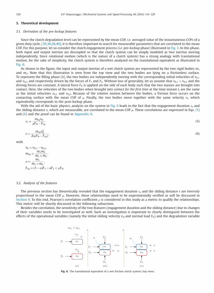
Since the clutch degradation level can be represented by the mean COF, i.e. averaged value of the instantaneous COFs of agiven duty cycle, [39,30,28,40], it is therefore important to search for measurable parameters that are correlated to the meanCOF. For this purpose, let us consider the clutch engagement process (i.e. pre-lockup phase) illustrated in Fig. 3. In this phase,both input and output inertias are decoupled so that the clutch system can be simply modeled as two inertias movingindependently. Since rotational motion (which is the nature of a clutch system) has a strong analogy with translationalmotion, for the sake of simplicity, the clutch system is therefore analyzed on the translational equivalent as illustrated inFig. 6.

As shown in the figure, the input and output inertias of a wet clutch system are represented by the two rigid bodies m1

and m2. Note that this illustration is seen from the top view and the two bodies are lying on a frictionless surface.To represent the filling phase (ii), the two bodies are independently moving with the corresponding initial velocities of v0;1and v0;2 and respectively driven by the forces of F1 and F2. Without loss of generality, let us assume that v0;14v0;2 and thedriving forces are constant. A lateral force FN is applied on the side of each body such that the two masses are brought intocontact. Here, the velocities of the two bodies when brought into contact for the first time at the time instant ti are the sameas the initial velocities v0;1 and v0;2. Because of the relative motion between the bodies, a friction force occurs on thecontacting surface with the mean COF of μ. Finally, the two bodies move together with the same velocity vl, whichequivalently corresponds to the post-lockup phase.

With the aid of the basic physics, analysis on the system in Fig. 6 leads to the fact that the engagement duration τe andthe sliding distance s, which are measurable, are correlated to the mean COF μ. These correlations are expressed in Eqs. (5)and (6) and the proof can be found in Appendix A.

τe ¼meqv0

μFN�Feqð5Þ

s¼ meqv202ðμFN�FeqÞ

; ð6Þ

with

v0 ¼ v0;1�v0;2;

meq ¼m1m2

m1þm2;

α¼ m1

m1þm2;

Feq ¼ ð1�αÞF1�αF2omFN :

3.2. Analysis of the features

The previous section has theoretically revealed that the engagement duration τe and the sliding distance s are inverselyproportional to the mean COF μ. However, these relationships need to be experimentally verified as will be discussed inSection 4. To this end, Pearson0s correlation coefficient ρ is considered in this study as a metric to qualify the relationships.This metric will be shortly discussed in the following subsection.

Besides the correlation, the sensitivity of the two features (engagement duration and the sliding distance) due to changesof their variables needs to be investigated as well. Such an investigation is important to clearly distinguish between theeffects of the operational variables (namely the initial sliding velocity v0 and normal load FN) and the degradation variable

Fig. 6. The translational equivalent of a wet friction clutch system (top view).

A.P. Ompusunggu / Mechanical Systems and Signal Processing 46 (2014) 114–128 121

(namely the mean COF μ) on the behavior of both features. This understanding can aid in developing a strategy for realizingan accurate clutch monitoring system.

Remark 1. Unlike the engagement duration feature τe, the computation of the sliding distance feature s from measurementsignals (i.e. discrete data) has not been discussed yet in the previous sections. Assume that the (discrete) signal of interestωr;ljsoi, l¼ 1;2;…;N, obtained from the procedure described in Fig. 5, is given. Hence, the sliding distance s can be computedfrom the signal of interest by the following equation:

s¼ τs ∑L

l ¼ 1ωr;ljsoi; ð7Þ

where τs denotes the sampling period and LoN is determined based on Eq. (3).

3.2.1. Correlation analysis: Pearson0s correlation coefficientAssume that two discrete quantities, xi and yi, i¼ 1;2;…;N, are obtained from a set of experiments. Pearson0s correlation

coefficient ρ of the two quantities is mathematically defined as [43]

ρ¼ ∑Ni ¼ 1ðxi�xÞðyi�yÞffiffiffiffiffiffiffiffiffiffiffiffiffiffiffiffiffiffiffiffiffiffiffiffiffiffiffiffiffi

∑Ni ¼ 1ðxi�xÞ2

q ffiffiffiffiffiffiffiffiffiffiffiffiffiffiffiffiffiffiffiffiffiffiffiffiffiffiffiffiffi∑N

i ¼ 1ðyi�yÞ2q ; ð8Þ

with

x ¼ 1N

∑N

i ¼ 1xi; ð9Þ

y ¼ 1N

∑N

i ¼ 1yi: ð10Þ

Eq. (8) implies that the values of the correlation coefficient lie between �1 and þ1. When the values of the coefficient areclose to �1, it is known that the dependency between two variables is inversely proportional. On the other hand, thedependency is linearly proportional when the values are close to þ1.

3.2.2. Sensitivity analysisLet us reevaluate the expressions of the engagement duration τe and sliding distance s given in Eqs. (5) and (6)

respectively. The total derivatives of τe and s in function of all relevant variables μ; FN ; v0 and Feq can be formulated asfollows:

dτe ¼∂τe∂μ

dμþ ∂τe∂FN

dFNþ∂τe∂v0

dv0þ∂τe∂Feq

dFeq; ð11Þ

and

ds¼ ∂s∂μ

dμþ ∂s∂FN

dFNþ∂s∂v0

dv0þ∂s∂Feq

dFeq: ð12Þ

By solving the latter equations with the help of Eqs. (5) and (6), one can show that the total derivatives of τe and s can beexpressed as follows:

dτe ¼ τe � dμμð1�βÞ �

dFNFNð1�βÞ þ

dv0v0

þ dFeqFeqð1=β�1Þ

� �; ð13Þ

and

ds¼ s � dμμð1�βÞ �

dFNFNð1�βÞ þ

2dv0v0

þ dFeqFeqð1=β�1Þ

� �; ð14Þ

with

0oβ¼ FeqμFN

o1:

For large changes, Eqs. (13) and (14) can be rewritten as follows:

Δτeτe

¼ � Δμμð1�βÞ �

ΔFNFNð1�βÞ þ

Δv0v0

þ ΔFeqFeqð1=β�1Þ ; ð15Þ

and

Δss

¼ � Δμμð1�βÞ �

ΔFNFNð1�βÞ þ

2Δv0v0

þ ΔFeqFeqð1=β�1Þ : ð16Þ

A.P. Ompusunggu / Mechanical Systems and Signal Processing 46 (2014) 114–128122

It is clear now from Eqs. (15) and (16) that variations of the two features (Δτe and Δs) have a negative correlationwith variationsof the mean COF Δμ and the normal force ΔFN . On the other hand, variations of the two features have a positive correlation with avariation of the initial relative velocity Δv0 and the external force ΔFeq. Surprisingly, a variation of the initial sliding velocity Δv0gives a two times larger on the variation of the sliding distance Δs compared to that of the engagement time Δτe.

For clutch condition monitoring purposes, where the change of degradation level (state) that is represented by the mean COFμ is tracked based on feature is of interest, the variations of the operational variables, namely pressure variation Δp (equivalent toΔFN), variation of the initial relative rotational velocity Δωtrig (equivalent to Δv0) and variation of the input and output torqueΔMi;ΔMo (equivalent to ΔFeq), should be minimized in order to achieve an accurate assessment of the clutch condition.One possible strategy to realize this is by embedding the aforementioned control routine in the ECU, where the control signalsent to the control valve for a clutch actuation is triggered if the pre-defined initial relative velocity ωtrig is detected. In terms ofminimizing the variation of the applied normal force (pressure) Δp, the control signal sent to the valve should be kept the same.

Depending on the type of the used oil/automatic transmission fluid (ATF), a variation of the oil temperature ΔT can havea significant contribution to the variation of the mean COF Δμ. Thus, when monitoring the condition of a wet clutch usingthe proposed features is of interest, the oil temperature variation should be minimized in order to achieve an accurateassessment. In practice, controlling the oil temperature of a wet clutch to a certain value is a difficult task. However,minimizing the oil temperature variation for clutch condition monitoring purpose is still feasible by embedding anacquisition routine in the ECU, where all the relevant signals are only recorded and processedwhen the oil temperature lies ina certain temperature range. This suggests that the use of a temperature sensor has an added value for realizing an accuratecondition monitoring system based on the proposed method.

Ideally, if variations of all the operational variables (Δωtrig , Δp, ΔMi, ΔMo and ΔT) are negligible, the relationshipsbetween the two features and the mean COF become simple:

Δss

¼ Δτeτe

¼ � Δμμð1�βÞ ; ð17Þ

4. Experimental verification and discussions

To experimentally verify the theory developed in the previous section, the first four datasets used in the previousinvestigations [15,16] are reanalyzed in this paper. Notice that the data are obtained from accelerated life tests (ALTs) carriedout on different commercial wet friction clutches using a fully instrumented SAE#2 test setup under the same operatingconditions (laboratory environment). All the tests were carried out until 10,000 duty cycles with relatively high energydissipation. For further description of the experiments, interested readers are referred to [15,16].

During the tests, the initial input and output rotational velocities, i.e. ωi;trig and ωo;trig , applied pressure p and inlet oiltemperature Tinlet were controlled at approximately the same corresponding values for each clutch duty cycle. In addition,no torques were applied on the input and output flywheels, i.e.Mo ¼Mi ¼ 0. In this way, the contribution of any variations ofthe operational variables to the variations of the two features is expected to be negligible. Hence, any variations of the twofeatures are mainly due to the degradation occurring in the clutches. Fig. 7 shows the histograms of the mean values of theoperational variables for different duty cycles. As can be seen in Table 1, the variations in percentage of the operationalvariables are in general less than 5%.

4.1. Verification of the features behavior

By applying the feature extraction procedure described earlier, the two features can be computed from the signal ofinterest. It is important to note here that the signals of interest for different duty cycles and ALTs can be found in [15].Additionally, the procedure to compute the mean COF from relevant signals for every duty cycle is also discussed therein.

Fig. 8 shows the evolution of the features and the mean COF in a function of the duty cycles obtained from different ALTs.It is seen from the figure that as the degradation progresses the mean COFs drop which confirm experimental evidencereported in the literature, for example see Refs. [30,40]. Furthermore, one can clearly see that the trend of the mean COF isopposite from the trends of the two features. Hence, this experimental evidence confirms that the theoretical predictionsdiscussed in Section 3 are verified.

Remarkably, the trends of the features show a (quasi) linear behavior with relatively small variations. These smallvariations are theoretically plausible since the variations of the operational variables are relatively small (i.e. less than 5%) asshown in Table 1. Hence, as expected, the trends are mainly due to the clutch degradation. For comparison purposes, thefeatures (τe and s) and the mean COF μ are normalized according to the following equations:

μ ¼ μ�μref

μrefð18Þ

τe ¼τe�τrefe

τrefe

ð19Þ

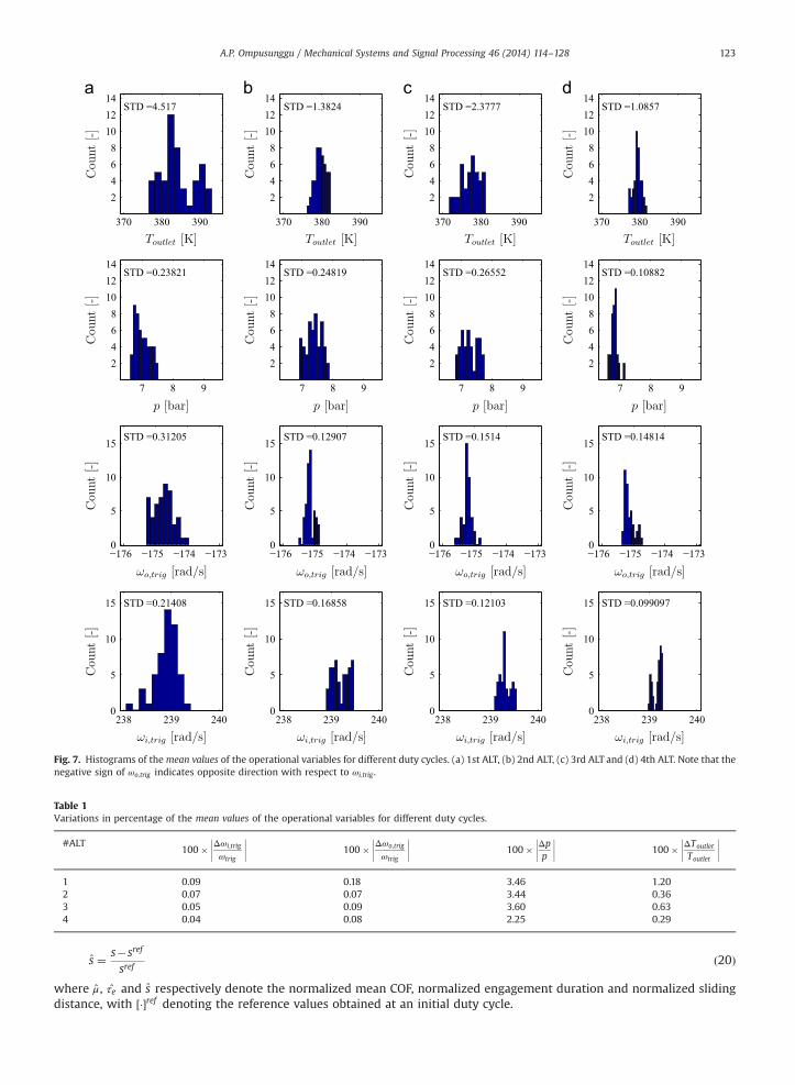
Table 1Variations in percentage of the mean values of the operational variables for different duty cycles.

#ALT100� Δωi;trig

ωtrig

�������� 100� Δωo;trig

ωtrig

�������� 100� Δp

p

�������� 100� ΔToutlet

Toutlet

��������

1 0.09 0.18 3.46 1.202 0.07 0.07 3.44 0.363 0.05 0.09 3.60 0.634 0.04 0.08 2.25 0.29

Fig. 7. Histograms of themean values of the operational variables for different duty cycles. (a) 1st ALT, (b) 2nd ALT, (c) 3rd ALT and (d) 4th ALT. Note that thenegative sign of ωo;trig indicates opposite direction with respect to ωi;trig .

A.P. Ompusunggu / Mechanical Systems and Signal Processing 46 (2014) 114–128 123

s ¼ s�sref

srefð20Þ

where μ, τe and s respectively denote the normalized mean COF, normalized engagement duration and normalized slidingdistance, with ½��ref denoting the reference values obtained at an initial duty cycle.

Fig. 8. Comparison of the evolution of the mean COF μ and the two features (engagement duration τe and sliding distance s) for different duty cycles.(a) Absolute values and (b) normalized values.

A.P. Ompusunggu / Mechanical Systems and Signal Processing 46 (2014) 114–128124

Fig. 8(b) shows the evolution of the normalized features and the mean COF. As can be seen in the figure, the absolutechanges of the two normalized features (τe and s) after 10,000 duty cycles are the same for the four ALTs as theoreticallypredicted, but the absolute changes of the normalized mean COF μ are larger than those of the two normalized features.Nevertheless, the absolute changes of the three normalized quantities after 10,000 duty cycles are in the same order ofmagnitude, thus reasonably confirming Eq. (17).

4.2. Correlation analysis

In order to verify the theoretical relationships between the features and the mean COF discussed previously, thecorrelation coefficients of τe vs. μ and s vs. μ according to Eq. (8) have been computed for different ALTs. Fig. 9 showsthe experimental correlations of the two normalized features with the normalized mean COF. Visually, it is obvious from thefigure that the relationships are inversely proportional. The relationships are verified by the correlation coefficient values,which are very close to �1, as listed in Table 2.

5. Concluding remarks

The theoretical derivation of the pre-lockup features useful for wet friction clutch condition monitoring is discussed inthis paper. It is shown theoretically that the two pre-lockup features are inversely proportional to the mean coefficient offriction (COF). To verify the theoretical predictions, Pearson0s correlation coefficients have been computed on theexperimental data obtained from accelerated life tests of some commercial wet friction clutches using a fully instrumentedSAE#2 test setup. The values of the coefficient are very close to �1, thus verifying the theoretical predictions.

In order to achieve an accurate condition monitoring method, it is theoretically revealed that the variations of someoperational variables, namely (i) the oil temperature, (ii) actuation pressure and (iii) initial relative rotational velocity,should be kept as small as possible. For practical implementation, this can be realized by embedding some control andacquisition related-routines into the Engineering Control Unit (ECU) that can satisfy the aforementioned requirements.The nature of the proposed signal processing and feature extraction implies that the pre-lockup features are suitable forcondition monitoring of wet friction clutches used in both traditional automatic transmissions (ATs) and dual clutch

Table 2Correlation coefficients of τe vs. μ and s vs. μ for different ALTs.

#ALT ρ1 : τe vs. μ ρ2 : s vs. μ

1 �0.994 �0.9922 �0.994 �0.9933 �0.989 �0.9894 �0.992 �0.989

Fig. 9. Experimental relationship of the two features (i.e. τe and s) vs. the mean COF μ obtained from (a) ALT#1, (b) ALT#2, (c) ALT#3 and (d) ALT#4. Notethat the marker □denotes ρ1: τe vs. μ and the marker ⋆ denotes ρ2: s vs. μ .

A.P. Ompusunggu / Mechanical Systems and Signal Processing 46 (2014) 114–128 125

transmissions (DCTs), where the initial relative rotational velocity can be imposed at (more or less) the same value fordifferent engagement cycles.

Acknowledgments

The author wishes to thank Dr. Mark Versteyhe of Dana Spicer Off Highway Belgium for sharing the experimental data.The author also gratefully acknowledges the two anonymous reviewers for their constructive comments on the manuscript.The scientific responsibility is assumed by its author.

A.P. Ompusunggu / Mechanical Systems and Signal Processing 46 (2014) 114–128126

Appendix A

The formal relationships of the engagement duration versus the mean COF (τe vs. μ) and the sliding distance versus themean COF (s vs. μ) expressed in Eqs. (5) and (6) can be summarized in Theorem 1.

Theorem 1. Let μ be denoting the mean COF of a clutch for a certain engagement cycle, and let τe and s be denoting theengagement duration and the sliding distance, respectively. Suppose that these three parameters are positive values. Thenτep1=μ and sp1=μ.

Proof. The equations of motion of the two bodies m1;m2 in Fig. 6, assuming v0;14v0;2, can be expressed as follows:

F1� f ¼m1dv1dt

; ðA:1Þ

F2þ f ¼m2dv2dt

; ðA:2Þ

with f ¼ μFN . By calculating the impulse of the driving force and the momentum of each body from the time instant ti to agiven time instant t, the instantaneous velocity of each body (v1; v2) can then be determined, i.e.:Z t

tiðF1�μFNÞ dt ¼

Z v1

v0;1m1 dv1; ðA:3Þ

v1 ¼ v0;1þðF1�μFNÞðt�tiÞ

m1; ðA:4Þ

Z t

tiðF2þμFNÞ dt ¼

Z v2

v0;2m2 dv2; ðA:5Þ

v2 ¼ v0;2þðF2þμFNÞðt�tiÞ

m2: ðA:6Þ

For the sake of simplicity, the time instant ti can be set to zero, so the velocities of the two bodies at given time instant t canbe rewritten as follows:

v1 ¼ v0;1þðF1�μFNÞt

m1; ðA:7Þ

v2 ¼ v0;2þðF2þμFNÞt

m2: ðA:8Þ

At the lockup time instant tl, the two bodies have the same velocity, i.e. v1 ¼ v2 ¼ vl. The time interval from ti to tl, which isreferred to as the engagement duration τe ¼ tl�ti, can be determined by equating Eq. (A.7) with Eq. (A.8). One can easilyshow that the engagement duration τe can be expressed according to the following equation:

τe ¼meqv0

μFN�Feq; ðA:9Þ

with

v0 ¼ v0;1�v0;2;

meq ¼m1m2

m1þm2;

α¼ m1

m1þm2;

Feq ¼ ð1�αÞF1�αF2:

Let vr be defined as the instantaneous relative velocity between the two bodies, i.e.

vr ¼ v1�v2: ðA:10ÞFurthermore, substituting Eqs. (A.7) and (A.8) into Eq. (A.10), the relative velocity vr can then be expressed as

vr ¼ v0þF1m1

� F2m2

� �t� μFN

meqt: ðA:11Þ

Let us now define the sliding distance s as the total relative displacement between the two bodies from the time instant ti totl. Mathematically, the sliding distance s can be calculated by integrating the relative velocity vr over the time interval, i.e.

s¼Z tl

tivr dt ¼

Z τe

0vr dt: ðA:12Þ

Fig. B1. A scheme illustrating the relationship between the coefficient of friction (COF) μ and the sliding distance s of a simple tribological system. Note thatμ0oμ.

A.P. Ompusunggu / Mechanical Systems and Signal Processing 46 (2014) 114–128 127

Solving Eq. (A.12) with the aid of Eqs. (A.9) and (A.11), one can show that the sliding distance s is expressible as follows:

s¼ meqv202ðμFN�FeqÞ

; ðA:13Þ

Appendix B

To further illustrate the correlations of the mean COF vs. the engagement duration and the mean COF vs. the slidingdistance, the system of the two rigid bodies shown in Fig. 6 can be reduced into a single rigid body of equivalent mass meq

subjected to a constant driving force Feq lying on a surface as illustrated in Fig. B1(a). Assume without loss of generality thatthe contact between the body and the surface is established after the time instant ti and the mean COF μ between the bodyand the surface, at a given degradation level (say a healthy state), is constant. Moreover, let us assume that the body issubjected to a constant normal load, i.e. its own weight. Due to the friction, the rigid body will stop after havingdisplacement of s with respect to its initial position as schematically illustrated in Fig. B1(b).

Let us now consider another case wherein the rigid body is placed on another surface representing a degraded state of awet friction clutch, where the mean COF is lower than that in the healthy state (μ0oμ). It should be noticed that thisparticular case is relevant since the mean COF of a wet friction clutch typically decreases due to the progression of bothmaterial and oil degradation [40,44]. One can immediately deduce that the sliding distance in the latter state will be largerthan that of the healthy state, i.e. μ0oμ-s04s, compare Fig. B1(b) and (c). Equivalently, the engagement duration in thedegraded state will be longer than the one in the healthy state, i.e. μ0oμ-τ0e4τe.

References

[1] M. Versteyhe, IWT proposal (in Dutch), Technical Report, Dana-Spicer Off Highway, Belgium, 2011.[2] A.P. Ompusunggu, Intelligent monitoring and prognostics of automotive clutches (Ph.D. thesis), Katholieke Universiteit Leuven, Department of

Mechanical Engineering, Division PMA, Belgium, 2012.[3] T. Kugiyama, N. Yoshimura, J. Mitsui, Tribology of automatic transmission fluid, Tribol. Lett. 5 (1998) 49–56.[4] A. Haj-Fraj, F. Pfeiffer, Dynamic modeling and analysis of automatic transmissions, in: Proceedings of IEEE/ASME International Conference on

Advanced Intelligent Mechatronics, 1999, pp. 1026–1031.[5] A. Crowther, N. Zhang, D.K. Liu, J.K. Jeyakumaran, Analysis and simulation of clutch engagement judder and stick-slip in automotive powertrain

systems, Proc. Inst. Mech. Eng. Part D: J. Autom. Eng. 218 (12) (2004) 1427–1446. arXiv:http://pid.sagepub.com/content/218/12/1427.full.pdfþhtml.[6] J. Kim, Launching performance analysis of a continuously variable transmission vehicle with different torsional couplings, J. Mech. Des. 127 (2) (2005)

295–301.[7] J. Deur, J. Asgari, D. Hrovat, Modeling and analysis of automatic transmission engagement dynamics-nonlinear case including validation, J. Dyn. Syst.

Meas. Control 128 (2) (2006) 251–262.[8] Z. Sun, K. Hebbale, Challenges and opportunities in automotive transmission control, in: Proceedings of 2005 American Control Conference, vol. 5,

2005, pp. 3284–3289.[9] L. Glielmo, L. Iannelli, V. Vacca, F. Vasca, Gearshift control for automated manual transmissions, IEEE/ASME Trans. Mechatron. 11 (1) (2006) 17–26.[10] D. Kim, H. Peng, S. Bai, J.M. Maguire, Control of integrated powertrain with electronic throttle and automatic transmission, IEEE Trans. Control Syst.

Technol. 15 (3) (2007) 474–482.[11] T. Janssens, Dynamic characterisation and modelling of dry and boundary lubricated friction for stabilisation and control purposes (Ph.D. thesis),

Katholieke Unversiteit Leuven, Department of Mechanical Engineering, Division PMA, Belgium, February, 2010.

A.P. Ompusunggu / Mechanical Systems and Signal Processing 46 (2014) 114–128128

[12] B.Z. Gao, H. Chen, K. Sanada, Y. Hu, Design of clutch-slip controller for automatic transmission using backstepping, IEEE/ASME Trans. Mechatron. 16 (3)(2011) 498–508.

[13] M. Zhou, S. Zhang, J. Wen, X. Wang, Research on CVT fault diagnosis system based on artificial neural network, in: Vehicle Power and PropulsionConference, 2008, VPPC 008, IEEE, 2008, pp. 1–5.

[14] H. Kong, G. Ren, J. He, B. Xiao, The application of fuzzy neural network in fault self-diagnosis system of automatic transmission, J. Softw. 6 (2) (2011)209–216. http://dx.doi.org/10.4304/jsw.6.2.209-216.

[15] A.P. Ompusunggu, J.-M. Papy, S. Vandenplas, P. Sas, H. VanBrussel, Condition monitoring method for automatic transmission clutches, Int. J. Progn.Health Manag. (IJPHM) Soc. 3 (2012) 19–32.

[16] A.P. Ompusunggu, J.-M. Papy, S. Vandenplas, P. Sas, H. VanBrussel, A novel monitoring method of wet friction clutches based on the post-lockuptorsional vibration signal, Mech. Syst. Signal Process. 35 (2013) 345–368.

[17] R.K. Mobley, An Introduction to Predictive Maintenance, Butterworth-Heinemann, 2002.[18] M. Basseville, A. Benveniste, B. Gach-Devauchelle, M. Goursat, D. Bonnecase, P. Dorey, M. Prevosto, M. Olagnon, In situ damage monitoring in vibration

mechanics: diagnostics and predictive maintenance, Mech. Syst. Signal Process. 7 (5) (1993) 401–423.[19] D. Bansal, D.J. Evans, B. Jones, A real-time predictive maintenance system for machine systems, Int. J. Mach. Tools Manuf. 44 (7–8) (2004) 759–766.[20] M.C. Garcia, M.A. Sanz-Bobi, J. del Pico, SIMAP: Intelligent system for predictive maintenance: application to the health condition monitoring of a wind

turbine gearbox, Comput. Ind. 57 (6) (2006) 552–568.[21] J. Srinivas, B.S.N. Murthy, S.H. Yang, Damage diagnosis in drive-lines using response-based optimization, Proc. Inst. Mech. Eng. Part D: J. Autom. Eng.

221 (11) (2007) 1399–1404.[22] A. Bey-Temsamani, M. Engels, A. Motten, S. Vandenplas, A.P. Ompusunggu, A practical approach to combine data mining and prognostics for improved

predictive maintenance, in: The 15th ACM SIGKDD Conference on Knowledge Discovery and Data Mining, 2009.[23] A. Bey-Temsamani, M. Engels, A. Motten, S. Vandenplas, A.P. Ompusunggu, Condition-based maintenance for OEM0s by application of data mining and

prediction techniques, in: Proceedings of the 4th World Congress on Engineering Asset Management, 2009.[24] Y. Kato, T. Shibayama, Mechanism of automatic transmissions and their requirements for wet clutches and wet brakes, Jpn. J. Tribol. 39 (1994)

1427–1437.[25] R. Mäki, Wet clutch tribology—friction characteristics in limited slip differentials (Ph.D. thesis), Luleå University of Technology, Division of Machine

Elements, Sweden, 2005.[26] N. Sakai, F. Honda, K. Nakijima, Friction characteristics of wet paper clutch for automotive torque transmissions, Lubr. Eng. 49 (2) (1993) 97–101.[27] H. Gao, G.C. Barber, H. Chu, Friction characteristics of a paper-based friction material, Int. J. Autom. Technol. 3 (4) (2002) 171–176.[28] S. Li, M. Devlin, S.H. Tersigni, T.C. Jao, K. Yatsunami, T.M. Cameron, Fundamentals of anti-shudder durability: Part I clutch plate study, SAE Technical

Paper 2003-01-1983, 2003, pp. 51–62.[29] T. Newcomb, M. Sparrow, B. Ciupak, Glaze analysis of friction plates, SAE Technical Paper 2006-01-3244.[30] M. Maeda, Y. Murakami, Testing method and effect of ATF performance on degradation of wet friction materials, SAE Technical Paper 2003-01-1982,

2003, pp. 45–50.[31] D. Wooton, The lubricant0s nemesis—oxidation, in: Practicing Oil Analysis Magazine, 2007.[32] G. Livingstone, D. Wooton, B. Thompson, Finding the root causes of oil degradation, in: Practicing Oil Analysis Magazine, 2007.[33] M. Duncanson, Detecting and controlling water in oil, in: Practicing Oil Analysis Magazine, 2005.[34] M.F. Smiechowski, V.F. Lvovich, Electrochemical monitoring of water surfactant interactions in industrial lubricants, J. Electroanal. Chem. 534 (2)

(2002) 171–180.[35] B. Wright, J.P.R. du Parquet, Degradation of polymers in multigrade lubricants by mechanical shear, Polym. Degrad. Stab. 5 (1983) 425–447.[36] I.I. Kudish, R.G. Airapetyan, Lubricants with non-newtonian rheology and their degradation in line contacts, J. Tribol. 126 (1) (2004) 112–124.[37] K. Berglund, Sustainable performance of wet clutch systems (Master0s thesis), Luleå University of Technology, Department of Applied Physics and

Mechanical Engineering, Division of Machine Elements, 2010.[38] J.J. Guan, P.A. Willermet, R.O. Carter, D.J. Melotik, Interaction between ATFs and friction material for modulated torque converter clutches, SAE

Technical Paper 981098, 1998, pp. 245–252.[39] K. Matsuo, S. Saeki, Study on the change of friction characteristics with use in the wet clutch of automatic transmission, SAE Technical Paper 972928,

1997, pp. 93–98.[40] J. Fei, H.-J. Li, L.-H. Qi, Y.-W. Fu, X.-T. Li, Carbon-fiber reinforced paper-based friction material: study on friction stability as a function of operating

variables, J. Tribol. 130 (4) (2008) 041605.[41] A.P. Ompusunggu, P. Sas, H. VanBrussel, Modeling and simulation of the engagement dynamics of a wet friction clutch system subjected to

degradation: an application to condition monitoring and prognostics, Mechatronics 23 (6) (2013) 700–712.[42] A.P. Ompusunggu, S. Vandenplas, P. Sas, H. VanBrussel, Health assessment and prognostics of automotive clutches, in: First European Conference of

the Prognostics and Health Management Society, PHM Society, 2012.[43] J.L. Rodgers, W.A. Nicewander, Thirteen ways to look at the correlation coefficient, Am. Stat. 42 (1) (1988) 59–66.[44] A.P. Ompusunggu, T. Jannsens, P. Sas, Friction behavior of a wet clutch subjected to accelerated degradation, ISRN Tribol. 2013 (2013). ID 607279, 11

pages. http://dx.doi.org/10.5402/2013/607279.