Mechanical Simulation in AutoCAD 2012 - Autodeskaucache.autodesk.com/au2011/sessions/4324/class_handouts/v1_AC4… · Mechanical Simulation in AutoCAD® 2012 2 Introduction I consider

Mechanical Simulation in AutoCAD® 2012 Craig A. Miller – Pennsylvania College of Technology

AC4324 This class is designed to teach specific techniques for combining 3D AutoCAD blocks, parametric constraints, and parametric dimensions to develop AutoCAD assemblies that can be used to simulate motion of mechanical systems. You will learn how to expand the use of 2D parametric constraints into the 3D world to create complex AutoCAD assemblies. You will learn to apply parametric dimensions that will allow you to test assemblies at their extremes of motion and perform interference checking to ensure that the systems will perform as required when manufactured. The class will start with motion contained in a single plane, but will quickly advance to show techniques for building assemblies containing motion in multiple planes. We will conclude by showing how simple LISP routines can be applied to drive motion within mechanical systems built using the techniques learned in the class.

Learning Objectives At the end of this class, you will be able to:

Create a “skeleton frame” that is suitable for assembling blocks

Use parametric constraints to create mechanical assemblies

Apply parametric dimensions to assemblies to create motion

Drive motion within an assembly through the use of simple LISP routines

About the Speaker Craig Miller is currently employed as a CAD Technology Specialist and adjunct faculty member by the Pennsylvania College of Technology in Williamsport, PA. For the last 6 years, he has managed, developed, and taught courses for the College's Autodesk Authorized Training Center. He frequently works with area companies to help them achieve greater efficiencies with their CAD systems by customizing the applications for their specific industries. Prior to going to work for the College, he was employed as an Applications Engineer for Thermal Product Solutions designing custom heat treat oven systems for companies worldwide. He holds Autodesk Professional Certifications in both AutoCAD and Inventor.

[email protected]

Mechanical Simulation in AutoCAD® 2012

2

Introduction I consider myself fortunate in my position at the Pennsylvania College of Technology, to have access to

some of the most talented CAD users ever to draw a line between two points. Whether it is a member of

the Penn College faculty who has used AutoCAD since release 2.1, or an industry professional who has

been using AutoCAD nearly every day for the past 20 years, I have learned, gained, and been inspired to

push the boundaries of what I thought was possible with this program. This class is a direct result of

questions and ideas presented to me by the people whom I work with and for. I believe that the content

that follows is a unique combination of AutoCAD

techniques and tools that will allow users to simulate

mechanical systems in a way that was previously

thought only possible in software such as Inventor. I

am fairly certain that Autodesk never intended for

AutoCAD’s 2D geometric constraints to be used in the

3D world. Yet as we spend the next 90 minutes

building, moving, and animating several different

mechanical assemblies in AutoCAD, you will see that

sometimes unintended uses for tools are often some

of the best.

Geometric Constraints It will be necessary to begin with a brief discussion of AutoCAD’s 2D geometric constraint tools. In

AutoCAD, the geometric constraints are a series of tools that, when applied to AutoCAD objects, ascribe

a particular behavior to the object or between multiple objects. For example: when you draw a line on the

screen at some random angle then place a horizontal geometric constraint to that line, the line will be

moved to become horizontal. (See Figure 1) In addition, this line now must behave as the applied

geometric constraint requires; i.e. it cannot be edited or rotated to be at any angle other than the 0 angle

as long as the horizontal constraint remains assigned to the line object.

Figure 1


3

Geometric constraints can also be assigned between two or more AutoCAD objects, effectively assigning

a relationship between the entities. Using the same horizontal constraint described above, we can assign

a horizontal relationship between the center points of two circle objects. (See Figure 2) When the

horizontal constraint is applied between the two circle centers, the second object center point moves to

be horizontally in-line with the first selected center. If we now attempt to move either circle, we will find

that the assigned horizontal constraint will force both circles to move, such that their centers remain in the

same horizontal line.

Figure 2

There are 12 different types of geometric constraints in AutoCAD. They are:

Perpendicular

Parallel

Horizontal

Vertical

Tangent

Smooth (G2)

Collinear

Concentric

Symmetric

Equal

Coincident

Fix Each constraint assigns its own unique behavior to drawing entities. Some of the constraints can only be

assigned to specific types of objects while others can only be applied to multiple entities in the drawing.

Regardless of the behavior assigned by a particular constraint, all constraints are applied in the same

basic manor described above. To save time, I am only going to call attention to the constraint types that

we will be using for the 3D work that follows. (You can get much more information on all of the constraints

listed above in the AutoCAD help system.)

When working with 3D models in AutoCAD, you can make use of all the 2D geometric constraints

available. However, several of the constraints distinguish themselves from the rest as being particularly

effective when attempting to assemble 3D models into a mechanism. These constraints are:

Coincident – Constrains two points to remain together or a point to remain touching another point on an object.

Collinear – Constrains two lines to lie along the same infinite line. (The lines do not need to be touching.)

Fix – Constrains a point on an object to remain fixed to a specific location on the World Coordinate System.


4

Rules for Assigning 2D Constraints to 3D Objects Through much trial and error, I have learned that when you attempt to place 2D constraints onto 3D

objects in AutoCAD, there are a couple of things you need to keep in mind. (Or to look at it another way…

things that AutoCAD is just not going to let you do.) These things are as follows:

1. Geometric constraints can only be applied in the XY plane. Even though two objects may reside

in the same plane, AutoCAD will not allow you to constrain the two objects together unless you

move the USC so that the XY plane is in the same plane as the two objects being constrained

together.

2. Move the objects to be constrained so that they reside in the same plane before attempting to

place constraints between them. AutoCAD will not automatically move an object from one plane

to another so that a constraint can be applied. It is up to the user to make sure that objects are

co-planer.

3. AutoCAD will not allow multiple geometric constraints to exist on a 3D object in differing planes.

(i.e. If you constrain two points together between a crank-shaft and a connecting rod, near the

front of the crank-shaft, AutoCAD will not allow you to move the UCS to the back of the crank-

shaft and constrain another connecting rod to the shaft, if the crank-shaft is one continuous entity

or block.)

These “rules” all sound very restrictive, but there are often creative ways to get around each of these

issues in order to establish the behavior that you are looking for in your assemblies.

3D Blocks & Connection Points When modeling each of the solid parts that will eventually make up my assembly, I generally like to

include reference geometry that can be used in the assembly process. I place the reference geometry

strategically within the component model at points that will serve to connect with other components in the

assembly. (See Figure 3)

Figure 3

Clevis Connection Point

Rod Centerline


5

Placing reference geometry within the model is not always necessary for assembly, but it is required often

enough that I usually create it even when it’s not absolutely needed. I also recommend placing your

reference geometry on a separate layer so that you can turn this layer on and off as needed. Your

assemblies tend to look a lot better when you don’t have a lot of points and lines running through each of

your components.

Once you have your part modeled, and appropriate reference points and geometry drawn in, you will want

to create a 3D block from your model. Be sure to include all of the reference geometry along with the solid

model when you create and name your block. When creating the 3D block, I generally do not worry about

where the base-point of the block falls on the model. However, I do try to avoid selecting a base-point that

is also going to serve as a connection point in the model. Doing so can sometimes cause confusion when

moving and assembling your 3D blocks into a mechanism.

Assembly Finally, we start getting to the good stuff. It’s now time to start putting our assembly together. We will start

with a small assembly. The hydraulic cylinder shown in Figure 4 will be made up of two parts: a cylinder

body and a cylinder rod with clevis. I have added reference geometry to each of the solid models then

created blocks out of each, being sure to include the reference geometry in the 3D block. I have moved

both components so that the centerlines of each piece are in the XY plane. This will allow me to apply

geometric constraints between the two centerlines of each component.

Figure 4

I will begin by placing fixed constraints to the ends of the centerline of the component I wish to remain

stationary. In this case, I will choose the centerline endpoints of the cylinder body. WARNING: Before you

place any fixed constraints on any of the components in your assembly, you need to consider how this

component will move with respect to the rest of the parts in the assembly. In this example, if the cylinder

moves at all with respect to other components within the larger assembly, fixing the centerline as I am

doing here, would not be appropriate.


6

Next, I will place a collinear constraint between the centerline of the cylinder body and the centerline of

the cylinder rod. The rod should move to the cylinder body, such that the two centerlines of each

component are now collinear. The results of adding these two constraints are shown in Figure 5. Note the

constraint icons that appear next to the cylinder body.

Figure 5

At this point, you should be able to grab and drag the cylinder rod with your mouse. The rod will not move

dynamically, but you will be able to move the component while still maintaining the collinear relationship

between the two components.

Adding Parametric Dimensions Parametric dimensions represent another form of control over your AutoCAD geometry. They are placed

just like regular associative dimensions. However, unlike their associative counterparts, parametric

dimensions allow the user to edit their numerical value. Being able to change the value of a parametric

dimension allows us to modify the distance between the two pick-points used to place the dimension. If

the parametric dimension is attached to the endpoints of a line or between two circle centers, editing the

value of the dimension will allow us to change the length of the line or the distance between the two circle

centers. (See Figure 6)

Figure 6


7

The placement of parametric dimensions are subject to the same rules that must be followed when

placing geometric constraints. These rules are:

1. Parametric dimensions can only be applied in the XY plane.

2. Objects to which a parametric dimension is being applied must reside in the same plane.

(Ultimately this plane must also be the XY plane, so move your UCS if needed.)

3. AutoCAD will not allow multiple parametric constraints to exist on a 3D object in differing planes.

If we apply a parametric dimension to our cylinder model and place the dimension between the two clevis

attachment points, we should be able to vary the extension length simply by modifying the value of the

parametric dimension. You can vary the value of the parametric dimension either by double clicking on

the value of the dimension or by using the Parameters Palette. (See Figure 7)

Figure 7

To make your model look better, you can turn off the visibility of the geometric constraint icons and the

parametric dimensions. Note that if you turn off the visibility of the parametric dimensions, you will need to

rely on the Parameters Manager to control the position of your components in the assembly.

THAT’S IT!!! We have created our first simple assembly in AutoCAD and have successfully varied the

position of the components within the assembly by editing a parametric dimension. Let’s try something a

bit more interesting.

Develop a Skeleton Frame Another technique that you can use assemble models in AutoCAD is to build a skeleton frame from lines,

circles, arcs, etc. Once the geometry is complete, you will fix the skeleton model in place using fixed

geometric constraints. This technique is particularly useful when you need to assemble a system of parts

that interact in various planes. Let’s start simple though, with another planer example.

I have modeled a piston, connecting rod, and cam for a V-Twin motorcycle engine. I have also included

connection point geometry with each of the models and turned each component into a block that includes

each component’s connection geometry. Figure 8 shows each of the components with the connection

point geometry in place. The figure shows the parts in the X-ray visual style, which helps to show where

the connection point geometry is placed in each model. Take note of where I have positioned the


8

connection points on both the piston block and connection rod block. The points are placed on each of

these components to help take advantage of symmetry within the model.

Figure 8

To make the assembly of this system easier, I am going to

construct a skeleton frame model that will be used to help

place and guide the components. This particular skeleton

will be very simple. I will start by drawing two lines starting

at the origin to create a “V” with a 70 degree angle between

the two lines. To ensure that the two lines will not move

when you start assembling components to them using

geometric constraints, we will place fixed constraints to

both endpoints of each line. Finally, you may want to create

a new layer and place the skeleton frame on that layer so

that you can turn it on and off as needed. The completed

skeleton model is shown in Figure 9.

Figure 9

With the skeleton frame complete, we can now begin to assemble components to the frame. I’ll start by

placing the cam at the intersection of the two lines using a coincident constraint. Next, place a parametric

angle dimension between the reference line on the cam and one of the two fixed lines from the skeleton

frame. (This dimension will allow us to vary the position of the cam and change the positions of all

components in the assembly.) Next, I’ll place collinear constraints between the centerlines of the pistons

and the two angled lines of the skeleton frame. Finally, we will tie in the connecting rods by placing

coincident constraints between the appropriate points between the pistons, connecting rods, and cam.

Figure 10 shows one side of the assembly completed, ready to move on to the second piston/connecting

rod assembly.


9

Figure 10

After you have completed the assembly, turn off the layer that you created for the skeleton frame to clean

up the appearance of your model. You may also want to turn off the visibility of the constraint icons and

the parametric dimensions. Now open up the parameters manager and edit the value of the angular

parametric dimension. (It should be designated as ang1.) By changing this parameter value, you can vary

the position of the cam, as well as the connecting rods and pistons attached to it.

Figure 11

I’ll save the assembled model so that I can use it later

Complex Mechanical Linkages The next example involves several moving parts with sub-assemblies copied into the model from other

drawing files. For the backhoe arm, I have modeled all of the parts and have placed appropriate

connection points within each part in the form of points. Each piece of the assembly was turned into a

block object as in all of the previous examples. Each block was then inserted into the assembly and


10

positioned so that all of the connection points lie within the XY plane. I have also constructed an

extremely simple skeleton frame consisting of a single line with Fixed constraints placed on each

endpoint. This simple skeleton frame will serve in place of the tractor part of the model that I decided not

to construct. Figure 12 shows all of the block parts of the assembly, ready to be constrained together.

I’ll begin by placing coincident constraints between all of the appropriate connection points. (Remember

to pick first on the component that you want to remain stationary and second on the component that you

wish to move into position.) When finished the model should look like Figure 13.

Figure 12 Figure 13

Once the major components have been assembled, we are ready to introduce the hydraulic cylinder

components into the model. I have three different cylinders to place. Each one has been modeled in it’s

own separate drawing file and has one Collinear constraint applied that keeps the cylinder rod inline with

the cylinder body. I have avoided placing a dimensional constraint to control the stroke of the cylinder.

Avoiding this constraint will make the cylinder easier to place in the top level assembly. To get a copy of

the cylinder into the Backhoe Arm model, I will

use a simple copy and paste operation. The

copy/paste will bring with it all constraints that

exist between the components being being

copied. Let’s start with the boom cylinder

shown in Figure 14.

After copying the cylinder model into the top

level assembly, I’ll move the cylinder so that the

connection points of the cylinder lie in the same

plane as the connection points of the backhoe

arm components. Finally, we use coincident

constaints to assemble the cylinder into its

Figure 14


11

appropriate position within the system. When in position, the cylinder should look like Figure 15. We will

place the stick cylinder and the bucket cylinder using the same procedure. When all cylinders are in

position, the model should look like Figure 16.

Figure 15 Figure 16

It is at this point in the assembly that I will add the parametric dimensions that will allow me to control the

position of the components within the assembly. I will add three dimensions to the model. One for each of

the hydraulic cylinder components that will allow me to vary their stroke along with anything that they are

connected to. I will place the

parametric dimensions between the

connection points that I have setup in

the model. Because parametric

dimensions must obey the same rules

that the geometric constraints do, it is

necessary for me to make sure that the

dimensions are in the same plane as

the geometric constraints that have

already been placed on these

components. Figure 17 shows the

dimensional constraints placed on the

assembly. Note that I have chosen to

rename the constraint labels to make it

easier for me to distinguish which

dimension I am editing when changing

values in the Parameters Manager. Figure 17


12

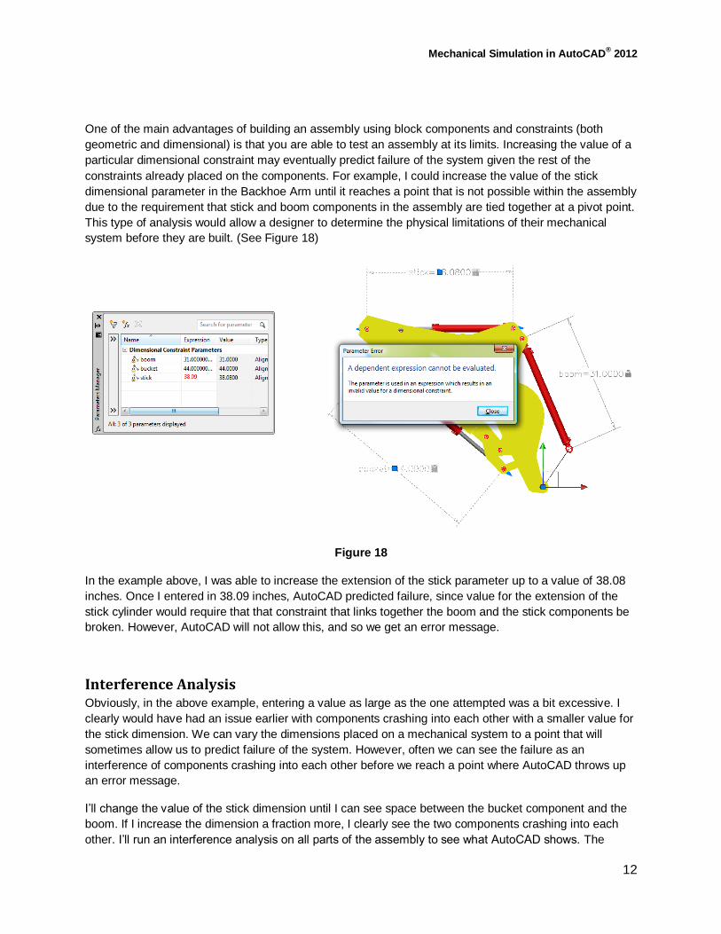
One of the main advantages of building an assembly using block components and constraints (both

geometric and dimensional) is that you are able to test an assembly at its limits. Increasing the value of a

particular dimensional constraint may eventually predict failure of the system given the rest of the

constraints already placed on the components. For example, I could increase the value of the stick

dimensional parameter in the Backhoe Arm until it reaches a point that is not possible within the assembly

due to the requirement that stick and boom components in the assembly are tied together at a pivot point.

This type of analysis would allow a designer to determine the physical limitations of their mechanical

system before they are built. (See Figure 18)

Figure 18

In the example above, I was able to increase the extension of the stick parameter up to a value of 38.08

inches. Once I entered in 38.09 inches, AutoCAD predicted failure, since value for the extension of the

stick cylinder would require that that constraint that links together the boom and the stick components be

broken. However, AutoCAD will not allow this, and so we get an error message.

Interference Analysis Obviously, in the above example, entering a value as large as the one attempted was a bit excessive. I

clearly would have had an issue earlier with components crashing into each other with a smaller value for

the stick dimension. We can vary the dimensions placed on a mechanical system to a point that will

sometimes allow us to predict failure of the system. However, often we can see the failure as an

interference of components crashing into each other before we reach a point where AutoCAD throws up

an error message.

I’ll change the value of the stick dimension until I can see space between the bucket component and the

boom. If I increase the dimension a fraction more, I clearly see the two components crashing into each

other. I’ll run an interference analysis on all parts of the assembly to see what AutoCAD shows. The


13

results are shown in Figure 19. Actually, AutoCAD predicts more interferences than I anticipated in this

example. You can cycle through to each of the interferences to determine if they are of concern or not. In

this case, the two interferences that I am most worried about occur between the bucket and the boom

parts and between the stick and the boom parts. Clearly, the current value of the stick dimension is not

going to work. Further, if I would start to change the value of the bucket cylinder, my interferences are

only going to get worse as the bucket rotates down and creates greater interferences between the bucket

and boom.

Figure 19

As a user, you can use a combination of these two techniques:

1. Vary values of parametric dimensions until failure is predicted.

2. Run interference checks on the system with parametric dimensions at their limits to test the

system for failure.

Track Assemblies The next example involves an object or a series of objects riding in a track. For this assembly, I have

developed a roll-up door consisting of several sections that ride in a track on each side of the assembly.

There are only six different components in this assembly. Three of them, the walls; floor slab; and roof,

are just there for aesthetics. Let’s take a closer look at how each of the “important” components of this

system are constructed.


14

First we will look at one of the door sections. It does not matter if we view a solid door section or a section

with windows. Both section types are built the same and contain connection points in them at the same

locations. Figure 20 shows a typical door section.

Figure 20

The door section has a 10ft x 2ft door section with two sets of rollers on each end to ride in a track. Note

the position of the connection points. The node points are located directly between roller positions on the

top and bottom sides of the door. I have also added small straight lines between the midpoints of the top

long edges of the door and the bottom long edges of the door. Note that all of my connection points are

located in a single plane. This is the most important aspect of the part. The connection points could have

been placed anywhere along the long edge of the door, as long as all of the connection point geometry

was drawn in the same plane.

Next, let’s take a look at the track component of this assembly. It is shown in Figure 21. This part was

built from two sweeps to create the tracks. The line geometry that is located between the two tracks will

serve as our connection point geometry for the door

sections. It is very important that the line geometry in

this part be constructed in a very specific way. First,

note the two short line segments and the single long

straight line segment that connects the two. These three

line segments will eventually serve as base points for

our parametric dimension. The dimension will allow us

to control the roll-up and roll-down position of the door

similar to how we controlled the position of components

in the Backhoe Arm assembly. The three line segments

will also serve as anchor points to allow us to fix the

position of the track component in the assembly. The

remaining part of the connection geometry that looks

like two straight line segments with a fillet between them

is actually a tightly controlled spline curve. This piece of

geometry will serve as the path our door sections need

to travel and, because of this, it needs to be a single

drawing entity. (Polylines will not work. I’ve tried them.)

Figure 21

Figure 21


15

Spline lines are viewed by AutoCAD as a single entity, but to achieve a path like the one shown in the

track component in Figure 21, you will need to use lots of control points. It’s not difficult, but it is

necessary.

Assembly of this multi-section door is a bit different

than anything that we have built to this point. I first

begin the assembly by placing a copy of the track

block into the model. I’ll place Fixed constraints to

each end of the long straight line that connects the

two shorter straight line segments. (See Figure 22)

After that, I’ll place the first of my door section blocks

in the assembly and move the component so that its

connection points lie in the same plane as the

connection point spline on the track component.

Finally, make sure that the XY plane is also the plane

that contains the connection point geometry. You can

either place the components so that this is true, or

you can use USC tools to move the XY plane into the

correct position.

Next, we will start to place coincident constraints

between the connection point spline on the track

component and the connection points on the door

section. You need to be careful here. When you

select the spline curve as a connection point, you will

want to use the <Object> option under the coincident

constraint to select the spline. This is because we

want the doors to move along the spline object and

not be coincident with a specific point. Do this two

times for each of the connection points in the door,

each time using the <Object> option before selecting

the spline. (See Figure 23)

Add each of the door sections to the model,

constraining each to the track component in the same

way that you did the first one above. Occasionally,

you may need to place a parametric dimension

between one of the doors and the track assembly in

order to move the doors around a bit. (It becomes

more and more difficult to move components around in an assembly as we continue to restrict their

movement with geometric constraints. Parametric dimensions seem to work pretty well to get parts to

move.)

Once you have at least two door sections placed in the assembly and constrained to the spline curve, we

can then attach the two sections together. In the real world, this is handled through either an offset hinge

attached to each door segment or a floating hinge, which is also attached to each door segment. Since I

did not model a hinge in my assembly, I will constrain the doors together using the short line segments

Figure 22

Figure 23


16

contained in the top and bottom faces of each door. The technique will be similar to applying a floating

hinge to the door sections. I will place a coincident constraint between the line object (be sure to use the

<Object> option of the coincident constraint command) contained on the top face of the door panel that

will be on the bottom part of a two panel assembly. My second selection will be the inside endpoint of the

line contained in the bottom face of the door panel that will be on top of the two panel assembly. (I hope

this makes some sense. Figure 24 shows the assembly before the constraint has been applied. Figure 25

shows the assembly after the constraint has been placed.)

Figure 24 Figure 25

You will need to do this for each door section that is added to your roll-up door assembly. The process is

tedious but, if done correctly, the result is pretty cool. The completed assembly is shown in Figure 26.

When you have each door section

assembled in the correct position

and each door panel is constrained

to the one adjacent, it will be

necessary to add a parametric

dimension to control the position of

the door. To accomplish this, I will

want to place the dimension so that

it is at an angle to the two “straight”

sections of the path. If not, it will

likely be difficult to control the

position of the door when it

approaches a nearly closed or

completely open position. Figure 27

shows where I choose to place the

parametric dimension to give me the

best chance to control the door

easily. It is not the only option, but it

should work.

Pick this Line First

Pick this Endpoint Second

Figure 26


17

After placing the dimension, edit the

dimension directly or from the Parameters

Manager to move the position of the door

up and down in its tracks.

The technique demonstrated in this

example has limitations. The first of these

is a restriction on the path. When

attempting to use a spline path in

AutoCAD, it is important that the path not

double back on itself. If the path has some

type of return bend in it, relative to the

parametric dimension being used to control

the position of the objects, you will only be

able to drive the objects up to the apex of

the return bend. Sometimes this limitation

can be overcome by carefully choosing the

location of the parametric dimension. A

second limitation to this path technique

involves animating the model. Later in this handout, I will demonstrate a technique for animating the

assembly using simple LISP routines. As we will learn, controlling the position of components along a

path with a consistent speed will become difficult when animating the assembly. It is difficult even in an

example as simple as the one used here.

Placing Constraints in Multiple Planes I mentioned earlier that AutoCAD will only allow constraints (both geometric and dimensional) to be

placed in the XY plane. So far all of the examples covered have been assembled so that their connection

points have fallen in a single plane. To apply the constraints we only needed to move the XY plane so

that it contained the connection points for the objects we were trying to assemble. However, it is possible

to create assemblies where all of the components are not located in single plane. Doing so sometimes

requires creativity and “out-of-the-box” thinking, but the end result is often worthwhile.

For this example, we will build a V-8

engine. To start, I have created a

skeleton model that will serve as a

basis for the assembly. (See Figure

28) After building the basic

geometry, I use the Fixed constraint

on the end of each line of the

skeleton frame to prevent the

geometry from moving. Note that it

would not be appropriate to turn the

skeleton frame into a block.

Although this would make it easier

to fix the geometry so that it would

Figure 27

Figure 28


18

not move, it would prevent us from assembling parts

to the frame in various planes. I have also placed the

skeleton frame geometry on a separate layer so that I

can control its visibility within the model.

Next, we can start to assembly engine parts to the

frame. The assembly consists of only three different

parts:

Connecting rod

Piston

Cam

All of the parts complete with their connection points

can be seen in Figure 29. This assembly is similar to

the V-Twin engine earlier, but becomes more

complicated due to the number of different planes

involved in the assembly. After inserting one copy of each block in the assembly, I’ll move the UCS to the

first piston assembly point on the skeleton frame. Next I’ll move each component to the origin of the

model so to that the connection points on each part in the in XY plane. Move the components off the 0,0,0

point. At this time, you may want to create multiple copies of the set of parts at each level in the model

where the components will need to be placed. (Creating copies of the parts now will save you lots of time

placing and moving components later.) After creating copies, return your attention to the very first set of

objects added to the model. Using the Coincident constraint, begin to assemble parts to the skeleton

frame and to each other. Be sure to use a Collinear constraint between the piston centerline and the

skeleton frame.

After assembling one cylinder, I’ll rotate the Cam

component into the position shown in Figure 30 and

place an Angular Parametric Dimension between

the connection point line in the Cam and one of the

angled lines in the skeleton frame. In this example,

I have chosen the same angled line as the one

used to control the linear travel of the piston. This

parametric dimension will fix the Cam’s position

along with the rest of the components constrained

to it. I also plan to use this angular dimension to

drive the rotation of the engine.

Next, we move the UCS to the next cylinder

position and assemble the next level of

components in much the same way as we did the

first. The only difference will be the Angular

Parametric Dimension that we will use to control the position of this next cylinder. For the position of the

cylinder, I will once again rotate the Cam to the same 90° position as I did the first. I’ll place the dimension

between the connection point line in the Cam and the angled skeleton frame line opposite the line that

Figure 29

Figure 30


19

was used to control the linear alignment of the

piston at this second cylinder position. For the

value of the dimension, I will include the

variable name of the first angular parametric

dimension so that it reads “ang1 + 45”. Now

when I edit the angle value of the first angular

parametric dimension, the second will update

with the first. This has the effect of constraining

the two Cams together such that they appear

to be acting as a single component. This

technique is what allows me to get around the

restriction of not being able to place constraints

on a single component in multiple planes. In

this case, each component is separate, but will

behave as one. (See Figure 31)

I’ll do one more. I’ll move my USC down to the next cylinder position and assemble components to each

other and to the frame. I’ll rotate the Cam part to the 90° position as before, then place an Angular

Parametric Dimension between the Cam and a line in the skeleton frame. This time the value of the

dimension will be “ang1 + 90”.

It’s just that easy! Let’s look at the completed model. (See Figure 32) You can use the Parameters

Manager to edit the value of the first angular dimension. If done correctly, the rest of the angular

parameters should be driven from the first.

Drive Motion within an Assembly Assembling a model and being able to manipulate components through the use of parametric dimensions

is helpful and can be a powerful tool when designing a mechanical system; however, it lacks the “cool

factor” of actually being able to animate your designs and see them move on the screen. Animating your

Figure 31

Figure 32


20

assemblies is also a great presentation tool. There is an understanding to be gained by seeing how the

mechanism will function in the real world once it is manufactured.

To my knowledge, there is no mechanism in AutoCAD that will allow you to animate an assembly easily.

For this reason, I have chosen to use a simple LISP routine consisting of a WHILE loop that changes the

value of a Parametric Dimension continuously from a start value to an ending value. The increment value

of the change can be increased or decreased easily within the program code. The great thing about using

LISP code is that anybody can do it, and you do not need to be an experienced LISP programmer to

make it happen.

Let’s start with a very simple example. I’ll open my original

Hydraulic Cylinder assembly. This assembly contains a single

linear Parametric Dimension with the variable designation of

“d1”. (See Figure 33) Next I’ll open the LISP routine that I will

use to drive the motion of this assembly. It is a text file that I

have named CEXTEND. The file is shown in Figure 34. I’m a

bit old school and like to write and edit my LISP routines in a

text editor like Notepad. It’s quick, simple, and it gets the job

done. Let’s break the program down line by line so that you

understand what it’s doing.

LINE 1: This line of the program defines a function (i.e. creates

a command) called cextend. It also declares a variable that I

have defined as “distance”.

LINE 2: This line of the program assigns a starting value to the variable “distance”. In this case, the

assigned value is 22 inches.

LINE 3: This line of the program starts a WHILE loop. A WHILE loop basically tells the program to repeat

the contents of the loop (whatever is in parenthesis) as long as the value of the variable “distance” is

less than or equal to 32 inches.

LINE 4: This line of the program is what changes the value of the “d1” distance parameter. It starts the

AutoCAD command “-parameters”, accesses the edit option (“e”), identifies the parameter to change

(“d”), and then assigns the current value of the variable “distance” to that parameter. Note that I have

used a “-“ before the command name. This tells AutoCAD to run the command line version of the

PARAMETERS command and does

not bring up the Parameters Palette;

which would be intrusive.

LINE 5: This line of the program

increments the value of the “distance”

variable by 0.0625.

LINE 6 & 7: These two lines close the

WHILE loop and finally the program.

Figure 33

Figure 34


21

That’s it! Type these simple lines into a text editor like Notepad, save the file with the extension .LSP, and

you are ready to go. Drag and drop the saved file into the AutoCAD window and type the name of the

function you created. In this case, I would type “cextend” at the command line and observe the results on

the screen.

You can modify the program above for just about any parameter that you want to animate. For example,

when I want to drive an angular parameter, I will often change the variable name “distance” to

something like “angle”. In line 4, I’ll change the parameter callout from “d1” to “ang1” (or any other

parameter name that I want to drive). The resulting program might be useful for animating a V-Twin

motorcycle engine. (See Figure 35)

You can increase or decrease the increment value in your programs to speed up or slow down the

animation. The smaller your increment value, the slower the animation; while the larger the value, the

faster your animation will become. You can also edit the value of your WHILE loop duration in Line 3 of

the program to change how long the program runs or the distance through which a parameter is driven.

Often, programs written to drive one assembly can be used without any changes to drive another

assembly. The program shown in Figure 35 is an example. We could drag and drop this program into our

V-8 engine assembly and drive this model without editing the program at all.

In assemblies where you have formula based parameters, you can drive one parameter and have another

that is parametrically linked to the one that you are driving animate as well. An example might be

something like a car jack as shown in Figure 36. In this example, I have linked the angle parameter that

controls the rotation of the screw to the parameters that control the height of the jack. (This is done in

AutoCAD.) For each revolution of the screw, the jack raises 1 inch. When the LISP routine that drives the

rotation of the screw is run, the parameters that control the height of the jack update as the rotation angle

increases via the program.

Figure 35


22

Finally, you can make your driving programs as complex as you like. In Figure 37, I show an example of a

slightly longer program that contains several WHILE loops in a particular order. I have also included a

REPEAT option that runs the contents of the WHILE loops four times before stopping. (i.e. This program

completes a series of WHILE loops that modify a set of parameters in a particular order. The program

then repeats these same steps four times before ending.) The program is called “DIG” and animates our

Backhoe Arm assembly.

Closing There is no question that creating, assembling, and animating AutoCAD models is more labor intensive

than it would be in a parametric modeler like Inventor. However, just knowing that this type of analysis

can be done in AutoCAD should open doors for mechanical designers who have not yet made the move

to Inventor. I have always been impressed with the unique and often unintended uses that AutoCAD

users find for the tools that have been added to AutoCAD over the years. I believe that the content of this

class and the examples that I have shown are yet another example of a use for AutoCAD that was

probably never intended.

Figure 36

Figure 37

Documents

Mechanical Simulation in AutoCAD 2012 - Autodeskaucache.autodesk.com/au2011/sessions/4324/class_handouts/v1_AC4… · Mechanical Simulation in AutoCAD® 2012 2 Introduction I consider