MECHANICAL ENGINEERING THERMAL AND FLUID SYSTEMS … · PE Mechanical – TFS – Fluid Mechanics with Hydraulic and Fluid Applications SECTION 01: Basic Information and Properties

PE Mechanical – TFS – Fluid Mechanics with Hydraulic and Fluid Applications www.SlaythePE.com

MECHANICAL ENGINEERING

THERMAL AND FLUID SYSTEMS

STUDY PROBLEMS

FLUID MECHANICS WITH

HYDRAULICS & FLUID APPLICATIONS

www.SlaythePE.com 1 Copyright © 2018. All rights reserved.

http://www.SlaythePE.com/


How to use this book

The exam specifications in effect since April 2017 state that approximately 6 problems from the “Fluid

Mechanics” topic will be in the morning “Principles” portion of your exam. The specifications also

state that approximately 24 problems comprise the “Hydraulic and Fluid Applications” portion of the

exam. You can expect, therefore, that Fluid Mechanics with Hydraulic and Fluid Applications will

occupy roughly 30 of the 80 problems (almost 40%) in the PE Mechanical Thermal-Fluid Systems

Exam. The problems in this book are designed to help you prepare for both of these broad topics.

Reviewing all the problems in this book will prepare you for these questions by focusing on exam-like

problems, recognizing the common pitfalls, and developing a solid understanding of the underlying

theories.

How it works

This study problems book works on what we call the “principle of progressive overload”. With this

technique you start with very easy problems and smoothly progress towards more complex problems.

A good example of progressive overload is the story of the famous wrestler Milo of Croton in ancient

Greece. This extraordinarily strong man was allegedly capable of carrying a fully grown bull on his

shoulders. He was reported to have achieved this tremendous strength by walking around town with a

new born calf on his shoulders every single day. As the calf grew, so did the man's strength.

We recommend you work the problems in this book in the order they are presented. Within each

section of the book, the first problems will feel “light”, like carrying that baby calf – you might even be

tempted to skip them. We strongly urge you to resist this temptation. As you progress, the problems

become harder, but the work you've been putting in with all the previous problems will bear fruit. You

will be pleasantly surprised at how relatively easy those “hard” problems will seem. You will soon be

carrying intellectual bulls on your shoulders! The problems that are considered “exam-level

difficult” are denoted with an asterisk.




This book is comprised of the following sections:

Sections Page

01: Basic Information and Properties of Fluids 5

02: Classification of Flows, Terminology & The Bernoulli Equation 19

03: Control Volume Analysis – Conservation of Mass & Energy 27

04: Control Volume Analysis – Conservation of Linear Momentum 35

05: External Flows: Flows over Immersed Bodies 39

06: Internal Flows: Friction Losses in Turbulent Flow in Pipes 47

07: Simple Pipe Networks 59

08: Turbomachines 69

09: Compressible Flow: Isentropic Flow & Nozzles 81

10: Compressible Flow: Normal Shock Waves 91

11: Answers 95

For the most part, these sections are not independent and build from the previous ones. We recommend

you go through them in the order presented, and be sure to review them all. Each section begins with a

brief discussion of the relevant concepts and equations. These discussions are laser-focused on the

aspects that are relevant to the P.E. exam and do not go into derivations with academic rigor.




This page was intentionally left blank




SECTION 01: Basic Information and Properties of Fluids

Physical quantities require quantitative descriptions when solving engineering problems. Consider the

density as one such quantity. It is a measure of the mass contained in a unit volume. However, density

is not considered a “fundamental” dimension. Only length, mass, time, temperature plus five more1 are

fundamental. All other quantities can be expressed in terms of fundamental dimensions. For instance,

the dimensions of force can be related to the fundamental dimensions of mass, length, and time. To

give the dimensions of a quantity a numerical value, a set of units must be selected.

All equations must be dimensionally homogeneous. That is, every term in an equation must have the

same units. If, at some stage of an analysis, you find yourself in a position to add two quantities that

have different units, it is a clear indication that something went wrong at an earlier stage. So checking

dimensions can serve as a valuable tool to spot errors. We strongly encourage you to always keep track

of units and never, ever, write down a number without its accompanying units. Lack of experience and

carelessness with units and unit conversions is one of the biggest hindrances towards success with the

P.E. exam.

Unity conversion ratios are identically equal to 1 and are unit-less, and thus such ratios (or their

inverses) can be inserted conveniently into any calculation to properly convert units, because any

quantity multiplied (or divided) by 1 remains unchanged. For example, the quantity:

∣ 1lbf

(32.174lbm⋅ft

s2 )∣is a ratio of two quantities that are identical, so it is equal to 1. Likewise, quantities such as:

∣12 in1ft ∣ ∣7.48052 gallons

1ft 3 ∣ ∣6.89476 kPa1 psi ∣

are all identically equal to 1 and are frequently inserted into calculations to ensure the dimensional

homogeneity of equations. Some books insert the archaic gravitational constant gc defined as

gc=32.174 lbm⋅ft /( lbf⋅s2 ) into equations in order to force units to match. This practice leads to

unnecessary confusion and is strongly discouraged. We recommend you instead use unity conversion

ratios.

1 The others are electric current, luminous intensity, plane angle, solid angle, and amount of substance.




When we say that equations must be dimensionally homogeneous, we mean that the dimensions of the

left side of the equation must be the same as those on the right side, and all additive separate terms

must have the same dimensions. We accept as a fundamental premise that all equations describing

physical phenomena must be dimensionally homogeneous. If this were not true, we would be

attempting to equate or add unlike physical quantities, which would not make sense. For example, the

equation for the velocity, V , of a uniformly accelerated body is:

V =V 0+at

Here we note that the dimensions of all three terms are length/time – thus, the equation is

dimensionally homogeneous. To illustrate the use of unity conversion ratios consider this example

(formatted in “PE style”):

EXAMPLE. The velocity of a uniformly accelerated body is given by V =V 0+at .Therefore, the velocity (inches per second) at t=0.25 min if the initial velocityV 0=50 ft /min and a=0.85ft /s2 is most nearly:(A) 50.85(B) 163(C) 815(D) 9780

The first way the careless test-taker messes this one up is by not writing down the units and doing the

following:

V =V 0+at=50+0.85×1=50.85

This is of course terribly wrong, but people actually do this! As you can see, 50.85 is one of the answer

choices. So, careless test-taker #1 would select (A) 50.85, and be wrong. The actual test will have

“distractor” answers like this. Be careful.

Careless test taker #2 does a little bit better, and actually gets a “correct” answer as follows:

V =V 0+at=50 ftmin

+0.85fts2 ×0.25 min

=50 ftmin

+0.85ft

s2 ×∣ 60 s1 min ∣

2

×0.25 min=50 ftmin

+765 ftmin

=815 ftmin

Note the use of the unity conversion factor on the second term, to ensure dimensional homogeneity of

the calculation. Note that 815 is one of the answer choices. However, the question specifies the units of

the answer must be in inches per second. Choosing (C) 815, would be wrong – even though the answer




is correct! We leave it as an exercise for you to confirm that the correct answer is (B).

Some valid equations contain constants with dimensions. For example, the equation for the distance, d ,

traveled by a body in free-fall can be written as:

d=16.1 t 2

and a check of the dimensions reveals that the constant 16.1 must have the dimensions of length over

time squared, if the equation is to be dimensionally homogeneous. This equation is actually a particular

case of the more general equation from physics for freely falling bodies:

d=gt 2

2

in which g is the acceleration of gravity. This equation is dimensionally homogeneous and valid in any

system of units, but for For g=32.2 ft /s2 the equation reduces to d=16.1 t 2 which is valid only for the

system of units using feet and seconds.

Pressure results from compressive forces acting on an area of a continuous medium. Pressure is a

scalar function; it acts equally in all directions at a given point for a fluid whether it is quiescent or in

motion.

The absolute pressure reaches zero when an ideal vacuum is achieved (i.e., in a space where there are

no molecules) thus negative absolute pressures are not possible. In addition to the absolute pressure

scale, pressures can be measured with respect to the local atmospheric pressure. The term gage-

pressure refers to values of pressure measured relative to the local atmospheric value. The gage-

pressure is negative whenever the absolute pressure is lower than the local atmospheric pressure.

Negative gage-pressure values are referred to as vacuum pressures. The following equation provides

the conversion from gage to absolute pressures:

pabsolute= pgage+ patm (1-1)

In the International System of Units (SI), pressure is measured in Pascals (Pa) with the SI prefixes

kilo-, Mega-, and Giga-, being among the most used in ordinary engineering applications.

1 kPa = 103 Pa

1 MPa = 103 kPa = 106 Pa

1 GPa = 103 MPa = 106 kPa = 109 Pa




The bar is a unit of pressure of the “metric system”, but is not formally approved as part of the SI. It is

defined as 100 kPa, or 0.1 MPa. In the US Customary System (USCS) of units, pressure is typically

expressed in pounds-force per square inch (lbf/in2, or psi) or pounds-force per square foot (psf).

In general, one of the words “absolute” or “gage” typically follows a value if the given pressure is

given as an absolute or gage pressure, respectively (e.g., “ p=750 kPa absolute”) but sometimes it is

specified in the units themselves, especially in the USCS. For example p=580 psia refers to an

absolute pressure of 580 pounds-force per square inch, and “ p=3.5psig ” refers to a gage pressure of

3.5 pounds force per square inch.

The local atmospheric pressure varies with elevation, and the “standard” value at sea level is defined as

101.3 kPa, 14.7 psi, 30 in. Hg, 760 mmHg, or 1.013 bar.

A fluid's density, ρ ,is defined as the mass of a unit of volume, and the specific volume, γ ,is defined

as the weight of a unit of volume:

γ =ρ g (1-1)

where g is the local gravity. The units of specific weight are N/m3 and lbf/ft3. The specific gravity SG is

often used to determine a fluid's density or specific weight. It is defined as the ratio of the density of a

substance to that of water at a reference temperature:

SG= ρρ water, std

= γγ water, std

(1-2)

If the reference temperature is the typically used value of 4°C then:

ρ water, std=1000kgm3

=62.4lbm ft3

=0.0361lbm in3

γwater, std=9810Nm3

=62.4 lbf ft3

=0.0361 lbf in3

For fluids at rest, it can be shown that the pressure does not vary in the horizontal plane (which is

defined as the plane normal to the gravity vector), and if we assume the density is constant then:

pγ +z=constant (1-3)

where z is positive in the vertically upward direction, so that pressure increases with depth. The

quantity ( p/ γ )+z is known as the piezometric head. If we define as z=0 the location of an interface

between the liquid and air above it (this is known as a free surface) at atmospheric pressure, then p=0

(gage) at z=0 , thus:

p=γ h (1-4)

where h is the depth below the free surface. Equation (1-4) is useful in converting pressure to an




equivalent height of liquid. For example, atmospheric pressure is often expressed in millimeters of

mercury – this means that the atmospheric pressure is equal to the pressure at a certain depth in a

mercury column, and by knowing the specific weight of mercury, we can determine the depth using

equation (1-4).

Manometers are instruments that use columns of liquid to measure pressures. Figure 1-1 shows a U-

tube manometer, which is used to measure relatively small pressures. In the figure, point “1” is located

in the center of a pipe that extends in the direction perpendicular to the page, and point “2” is at the free

surface of the right column, exposed to atmosphere.

Pipe

2

1

h

γ

Figure 1-1: U-tube Manometer.

We can use equation (1-3) to write:

p1+ γ z1= p2+γ z2

where the datum (i.e., the location where z=0 ) can be located anywhere we want. We know also that

p2=0 psig (we could also use p2= patm if we wish to work with absolute pressures). Choosing now

z1=0 , the above expression yields: p1= γ h .

Figure 1-2 shows a manometer that could be used to measure larger pressures since we could choose a

fluid with a large specific weight, γ B (for example if fluid 1 is water and fluid 2 – the red one – is

mercury, then γ B=13.6 γ A ). The pressure at location 1 can be determined by defining 4 points as

shown in Figure 1-2.




Pipe

4

1 H

h

2 3

γ B

γ A

Figure 1-2: U-tube Manometer with dedicated manometer fluid

We can use equation (1-3) to write:

p1+ γ A z1= p2+γ A z2

p3+ γ B z3= p4+ γ B z4

but, p2= p3 because points 2 and 3 are on the same horizontal plane ( z2=z3 ) and within the same

fluid. We can add the above equations to obtain:

p1+ γ A ( z1−z2 )=γ B ( z4−z3 )+ p4

and we can set p4=0 and work with gage pressures. The resulting expression for p1 is:

p1= γ B H −γ A h

Note that if fluid A (the one in the pipe) is a gas, and fluid B is a liquid, it generally follows that

γ A≪ γ B and the second term in the above expression can be safely neglected.

The lay person's understanding of viscosity is that it is related to the internal stickiness of a fluid. In

more technical terms, viscosity is linked to the rate of deformation of a fluid under shear stress. For a

given applied shear stress, a high viscosity fluid will experience smaller deformation than a low

viscosity fluid under the same stress.

Consider the fluid within a small gap between two concentric cylinders, as shown in Figure 1-3. An

externally applied torque causes the rotation of the inner cylinder, while the outer cylinder remains

stationary. The resistance to the rotation is due to the fluid's viscosity.




Rh

ω

Figure 1-3: Fluid being sheared between two cylinders: Fixed outer cylinder and rotating inner cylinder.

The fluid velocity u in the thin gap varies linearly2. The fluid layer adjacent to the inner cylinder will

have a velocity equal to the tangential velocity of the cylinder, ω R , where ω is the rotational speed of

the inner cylinder (in rad/s) and R is the radius of the inner cylinder. The fluid layer adjacent to the

outer (stationary) cylinder will be stationary. If the gap between the cylinders is h , then the velocity

gradient du/dr across the gap is (ω R)/h .

When a torque T is applied to the inner cylinder, the fluid in the gap experiences a shear stress τ ,

which is related to the velocity gradient:

τ =μ ∣dudr∣=μ (ω R)

h

Where the constant of proportionality between sheer stress and velocity gradient (in this very simple

flow) is the viscosity, μ .

Since the torque is:

T =stress×area×moment arm

T =τ ×2 π R L×R

or,

T = 2π R3ω L μh

(1-4)

Additionally, the power P, transmitted by a shaft rotating with an angular velocity ω by applying a

torque T is given by P=ω T , so inserting that into equation (1-4) we get:

2 If the gap width h is not small relative to R the velocity variation will not be linear.




P= 2π ω 2 R3 L μh

(1-5)

where we have neglected the stress acting on the ends of the cylinders. Since the torque depends on the

viscosity, this type of cylinder gap arrangement is used as a viscometer – a device used to measure

viscosity. If the shear stress in a fluid is directly proportional to the velocity gradient (shear strain rate),

the fluid is said to be a Newtonian fluid. If the shear stress varies in a non-linear way with the strain

rate, then the fluid is non-Newtonian (liquid plastics, blood, slurries, toothpaste, etc) and depending on

the functional form of this relationship the fluids are further classified as thixotropic, dilatant, Bingham

plastics, rheopectic, etc. Rheology is the branch of physics that deals with this study of deformation

and flow of materials.

From τ =μ ( du /dy ) it can be readily deduced that the dimensions of viscosity are force×time/length2.

Thus, in the USCS of units viscosity is given as lbf·s/ft2 and in SI units as N·s/m2. The poise (P) is an

alternatively used viscosity unit and 1 P = 0.1 N·s/m2. The poise is often used with the prefix “centi-”

because the viscosity of water at 20 °C is almost exactly 1 cP where 1 cP = 10-3 N·s/m2.

The group μ / ρ appears often in the derivation of equations, so it has become customary to give it a

name, kinematic viscosity:

ν =μρ (1-6)

and thus the viscosity μ is also referred to as “dynamic” viscosity. The dimensions of kinematic

viscosity are length2/time, and the USCS units are ft2/s and SI units are m2/s. The stoke3 (St) is an

alternatively used unit of kinematic viscosity and 1 St = 10 -4 m2/s. The stoke is often used with the

prefix “centi-” because the kinematic viscosity of water at 20 °C is almost exactly 1 cSt (10-6 m2/s).

Given a pressure change Δ p applied to a fluid, a packet of fluid with volume V will experience a

change in relative volume (ΔV )/V . The bulk modulus of elasticity, B gives the relative change in

volume for a given change in pressure applied to a fluid at constant temperature, T :

B= Δ p(Δ V )/V ∣

T

=ρ Δ pΔ ρ ∣

T

(1-7)

For gases, it can be shown that the bulk modulus is equal to the pressure. For liquid water at standard

conditions, the bulk modulus is roughly 310,000 psi – this means that to cause a 1% change in density

3 In the United States, it is more common to use the singular “Stoke”, but the unit is named after George G Stokes, hence in the rest of the world it is more common to hear “Stokes” as a unit of kinematic viscosity.




(i.e., (Δ ρ )/ ρ =0.01 ) of water, a pressure rise of 3,100 psi is required. The bulk modulus is also used

to determine the speed of sound c in a fluid:

c=√ Bρ (1-8)

which yields about 4,800 feet per second for the speed of sound in water at standard conditions.

PROBLEMS:

01-01. If V is a velocity, determine the dimensions of Z , α , and G , which appear in the

dimensionally homogeneous equation V =Z (α −1 )+G

01-02. The pressure difference, Δ p , across a partial blockage in an artery is approximated by the

equation:

Δ p=K v

μ VD

+K u( A0

A1

−1)2

ρ V 2

where V is the blood velocity, μ the blood viscosity, ρ the blood density, D the artery diameter, A0

the area of the unobstructed artery, and A1 the area of the blockage. Determine the SI dimensions of the

constants K v and K u .

01-03. A pressure of 4 psig is measured at an elevation of 6,560 ft – where the atmospheric pressure is

11.5 psia. What is the absolute pressure in (a) kPa, (b) mm of Hg, and (c) ft of water?

01-04. A gage reads a vacuum of 24 kPa. What is the absolute pressure (a) at sea level, and (b) at an

altitude of 4000 m where the atmospheric pressure is 0.616 bar?

01-05. Calculate the gage pressure (in psi) in a pipe transporting air if a U-tube manometer measures

9.85 inches of mercury. Note that the weight of air in the manometer is negligible.

01-06. If the air pressure in a pipe is 65 psig, what will a U-tube manometer with mercury indicate?




01-07*. The Weber number is a dimensionless parameter, given by:

We= ρ V 2 Lσ

where ρ is density, V is a velocity, L is a length, and σ is a material property of the fluid. Since the

Weber number is dimensionless, the units of σ must be:

(A) lbm/(ft·s)

(B) lbf/ft

(C) ft/lbf

(D) s2/lbm

01-08*. A formula to estimate the volume rate of flow, Q , flowing over a dam of length, B , is given

by the equation Q=3.09 B H 3/2 ,where H is the depth of the water above the top of the dam. This

formula gives Q in ft3/s when B and H are in feet. An equivalent formula that gives Q in gallons per

day when B and H are in feet is:

(A) Q=0.00027 B H 3/2

(B) Q=0.413 B H 3/2

(C) Q=3.09 B H 3/2

(D) Q=35,690 B H 3/2

01-09*. While performing a calculation, an engineer arrives at the following equation to calculate a

force: F=m V + p A , where m=600 kg / min , V =2 m /s , p=29.7 kPa , and A=50.3 cm2 .

Under these conditions, the force F (N) is most nearly:

(A) 35

(B) 169

(C) 1513

(D) 2694




01-10*. While performing a calculation, an engineer arrives at the following equation to calculate a

volumetric flow rate: Q=F /(ρ V ) ,where F=35 pounds-force, ρ =6.26 lbm /gallon , and V =15ft /s .

Under these conditions, the flow rate Q (cubic feet per hour) is most nearly:

(A) 0.373

(B) 12

(C) 5,775

(D) 43,172

01-11*. A heat transfer oil with a specific gravity of 0.86 flows through a pipe. The reading from a U-

tube manometer is 9.5 in Hg. The oil in the manometer is depressed 5 inches below the pipe centerline,

and the local atmospheric pressure is 14.7 psi. Under these conditions, the absolute pressure (psi) of the

oil in the pipe at the location of the manometer is most nearly:

(A) 4.5

(B) 7.8

(C) 14.7

(D) 19.2

01-12*. The pressure in the water pipe is 2.5 psig. The pressure (psig) in the oil pipe is most nearly:

(A) 1.0

(B) 2.0

(C) 2.2

(D) 4.5

Water

0.5 ftSG = 7.0

4.75 in

Oil, SG = 0.85




01-13*. The pressure in air pipe A is 15 psig. The pressure (psig) in air pipe B is most nearly:

(A) 6.2

(B) 10.6

(C) 14.6

(D) 15.0 Air pipe A

1.5 ft

Mercury30º

Air pipe B

01-14*. The reading of the pressure gage in psi is most nearly:

(A) a vacuum of 2.5

(B) a vacuum of 1.6

(C) a vacuum of 0.64

(D) 1.74

4 in

6 ft

Mercury

Water

Air




01-15*. The elevation difference h (ft) between the water levels in the two open tanks is most nearly:

(A) 0.13

(B) 1.6

(C) 2.6

(D) 3.5

SG = 0.9

Water Water

h

15.75 in.

01-16*. A 1 inch-diameter shaft is pulled through a cylindrical bearing as shown in the figure. The

lubricant that fills the 0.012-inch gap between the shaft and bearing is an oil having a kinematic

viscosity of 0.0086 ft2/s and a specific gravity of 0.91. The force required to pull the shaft at a velocity

of 10 ft/s is most nearly:

(A) 0.46

(B) 2.5

(C) 3.8

(D) 5.5 shaft

bearing

10 ft/s

1.65 ft




This page was intentionally left blank




Section 02: Classification of Flows, Terminology & The Bernoulli Equation

If in a given flow field the velocity vector only depends on one spatial coordinate (e.g., x, y, or z) we

say it is a one-dimensional flow. As examples, consider the flow pattern that occurs in long, straight

circular pipes or between parallel plates as shown in Figure 2-1. For the pipe flow, the velocity only

depends on the radial coordinate, r, and in the parallel plates case, the velocity only depends on the

vertical coordinate y.

u(r)

z

ru(y)

z

y

(a) (b)

Figure 2-1: One-dimensional flow: (a) flow in a pipe, (b) flow between parallel plates

In the cases above, even if the flow is unsteady (i.e. time-dependent, as in a startup or shutdown) the

flow would still be one-dimensional. The velocity profiles shown in Figure 2-1 can also be referred to

as fully developed flows, which means that the velocity profiles do not change in the direction of flow

(i.e., the z direction in the figure).

Many times in engineering applications considerable simplicity is achieved by invoking the assumption

of uniform flow, which implies that the velocity is constant over the cross-sectional area of the pipe or

conduit. The average velocity may change from one section to the other, but the flow conditions only

depend on the space variable in the direction of flow – as in Figure 2-2.

Figure 2-2: Uniform velocity profiles


V1 V

2



In a broad sense, a fluid flow may be classified as inviscid or viscous. An inviscid flow is one in which

the effects of the fluid's viscosity does not significantly influence the flow field, so these effects are

neglected. The primary class of flows that can be accurately analyzed as inviscid are external flows,

that is, flows that exist exterior to a solid body such as flow around an airfoil or a vehicle. Any viscous

effects that may exist are all within a very thin region adjacent to the surface of the solid body known

as a boundary layer. In many practical applications, the boundary layers are so thin that they can be

ignored when studying the gross, macroscopic features of a flow. Viscous flows include internal

flows, such as flows in pipes, conduits, and open channels. Viscous effects are responsible for the

“losses” encountered in these flows which we will examine in greater detail in further sections.

Viscous flows can be further classified as laminar or turbulent. In laminar flow, there is no significant

mixing of fluid particles with their neighboring particles. Imagine a set of “sheets” sliding past each

other. We recommend googling “laminar flow visualization” videos for some impressive

demonstrations of this feature. In many of these videos, you'll see a dye being injected in the flow. The

dye does not mix, retaining its “identity” for a relatively long time, over relatively long distances. The

flow may be time-dependent, or it may be steady. In a turbulent flow, quantities such as velocity and

pressure show random fluctuations with time and with the space coordinates. For turbulent conditions,

a flow is deemed “steady” if the time-averaged physical quantities (e.g., pressure, velocity,

temperature, etc) do not change in time. If you were to measure the velocity magnitude of a steady,

turbulent flow in a given location, you would notice an irregular pattern made by all the instantaneous

values, but they would all be “around” an average value that doesn't change with time. A dye injected

into a turbulent flow would quickly mix by the action of randomly moving particles.

The interaction of three key parameters defines if a fluid flow is laminar or turbulent. These three

parameters are the length scale, the fluid velocity scale, and the fluid's viscosity. The three parameters

are combined into a single dimensionless parameter (that can serve as a tool to make predictions about

the flow being laminar or turbulent) known as the Reynolds number:

Re= V Lν (2-1)

where V and L are a characteristic velocity and length, respectively, and ν is the fluid's kinematic

viscosity. If the Reynolds number is relatively low, the flow will be laminar; if it is large, the flow will

be turbulent. This phenomenon is quantified with the use of a critical Reynolds number, Recrit , so that




the flow is laminar if Re<Recrit . The magnitude of Recrit depends on the flow configuration, for

example for flow inside a rough walled pipe in most engineering applications, a value Recrit=2,000 is

typically used. A simple example of a transition from laminar to turbulent may be observed on the

smoke rising from a cigarette or a smoke stack. For a certain distance, the smoke rises in a smooth

(laminar) manner but then abruptly, the smoke mixes up and becomes turbulent and the narrow smoke

column widens and diffuses.

Finally, another flow classification distinguishes flows that are compressible from those that are

incompressible. An incompressible flow exists if the density of each fluid particle remains relatively

constant as it moves through the flow field. For most practical purposes, liquid flows are

incompressible. Also, under certain conditions involving minor pressure changes and low velocities,

gas flows may be considered incompressible. If the gas experiences relatively large density changes

which influence the flow, then it is compressible flow. For compressible flow, there is a great

distinction between flows involving velocities less than that of sound (subsonic flows) and flow

involving velocities greater than that of sound (supersonic flows).4 The Mach number is a measure of

the flow characteristic velocity relative to the local speed of sound:

M = Vc

(2-2)

where V is the gas speed and c is the local speed of sound. Thus, when M <1 the flow is subsonic, and

when M >1 the flow is supersonic. In gases, the speed of sound is given by c=√k RT where T is the

absolute temperature, k is a property known as the specific heat ratio, and R is the particular gas

constant.5 For air k=1.4 , and the gas constant is:

Rair={53.34 ft⋅lbf / lbm⋅°R0.3704 psia⋅ft 3/ lbm⋅°R640.08 psia⋅in3/ lbm⋅°R1,716.2 ft2 /s2⋅°R0.0686Btu / lbm⋅°R0.287 kJ / kg⋅K

}When M <0.3 it can be shown that density variations are not important so M<0.3 (which corresponds

roughly to a velocity under 300 ft/s or 100 m/s for standard air) is typically used as a criterion to decide

4 Sonic speed in air at 70°F (21.1°C ) is about 1,128 ft/s (343.9 m/s)5 For a thorough review of the ideal gas law please consult our Thermodynamics and Energy Balances ebook.




to model flow as incompressible without any significant loss of accuracy.

The well-known Bernoulli equation6 adopts the following form when applied between two points on

the same streamline:

V 12

2+

p1ρ +g z1=

V 22

2+

p2ρ +g z2 (2-3)

If we divide the equation above by g, it becomes:

V 12

2g+

p1γ +z1=

V 22

2g+

p2γ +z2 (2-4)

The term V 2/2 g is known as the velocity head and it represents the vertical distance needed for the

fluid to fall freely (neglecting friction) if it is to reach velocity V from rest. The term p / γ is known as

the pressure head, and it represents the height of a column of the fluid that is needed to produce the

pressure p . The elevation term z is related to the potential energy of the fluid and it is known as the

elevation head. The sum ( p/ γ )+z is called piezometric head, and the sum of all three terms is the

total head. The pressure is sometimes called static pressure and the group

pT= p+ρ V 2

2 (2-3)

is called the total pressure, or stagnation pressure. Consider the arrangement shown in Figure 2-3.

Here we see a pressure gage (or piezometer) mounted on the wall of a pipe or conduit, measuring the

static pressure at location 1. The probe on the right is a pitot-tube which is a thin, dead-end conduit

inserted in the flow. The fluid inside the tube (point 2) is stagnant.

Figure 2-3: Pressure probes: piezometer (for static pressure) and pitot tube (for total pressure).

6 This equation is obtained by applying F = ma along a streamline for steady, inviscid, incompressible flow.


p1 (static pressure) p

2 (total pressure)

21

pipe wall



If we apply Equation (2-3) from point 1 to point 2 we see that the pressure read by the pitot probe is the

stagnation pressure. The difference between the readings of the two probes can be used to determine

the velocity at point 1. Another device, known as a pitot-static probe combines both devices into one

instrument. The pitot-static probe provides the value of p2− p1 .

As an exercise, apply the Bernoulli equation between points 1 and 2 in Figure 2-3 to show that the

velocity at point 1 is given by:

V 1=√ 2ρ ( p2− p1 )

The Bernoulli equation can be used on many steady flow situations of engineering interest, as long as

viscous and compressibility effects are not important. Examples of external flows where the Bernoulli

equation is typically applied include determining the height of a jet of water, the force applied on

windows due to wind, or the surface pressure on a low velocity airfoil.

Examples of internal flows where the Bernoulli equation is typically applied involve internal flows

over short distances such as flow through contractions and flow from a plenum, nozzles and in pipes of

variable diameter for which the fluid velocity changes because the flow area is different from one

section to another. For these situations it is necessary to use the concept of conservation of mass (the

continuity equation) along with the Bernoulli equation. For a control volume in steady state,

conservation of mass requires that the rate at which the mass of fluid flows into the volume must equal

the rate at which it flows out of the volume (otherwise, mass would not be conserved). The mass flow

rate m (lbm/h, lbm/min, kg/h, etc) is given by m=ρ Q where Q is the volume flow rate (gal/min,

ft3/min, m3/s, etc). If at a given section the cross-sectional area is A , and the flow occurs across this

area (normal to the area) with an average velocity V the volume flow rate can be shown to be given by

Q=AV . If we label the inlet to the control volume as “1” and the outlet as “2”, then conservation of

mass requires: ρ 1 A1 V 1=ρ 2 A2V 2 . If the density remains constant, then ρ 1=ρ 2 and the above

becomes the continuity equation for incompressible flow:

A1 V 1=A2V 2 (2-4)

Refer to Figure 2-2. Here we see that a reduction in the cross sectional area brings about an increase in

the velocity.




PROBLEMS:

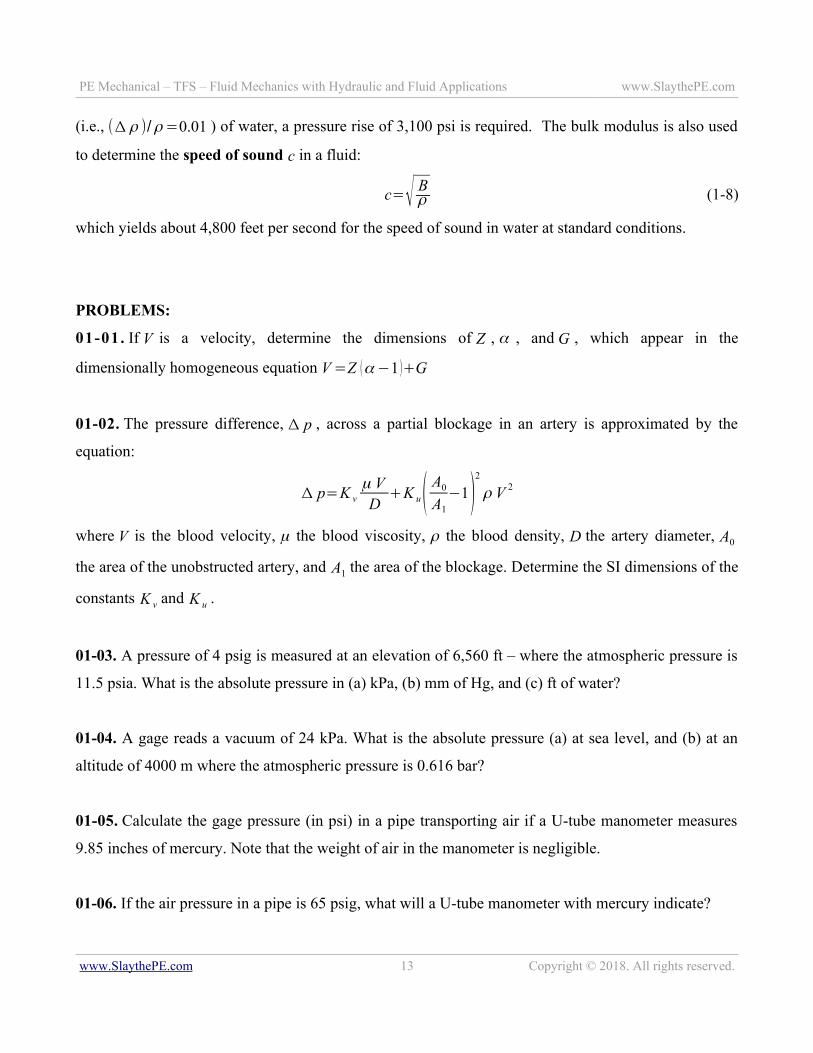
02-01. A 4-in. ID pipe carries 300 gpm of water at a pressure of 30 psig. Determine – in feet of water –

(a) the pressure head, (b) the velocity head, and (c) the total head with reference to a datum plane 20 ft

below the pipe.

02-02. Water flows at a rate of 300 gpm in a 4-inch, schedule-40, seamless steel pipe (ID=4.026

inches). The pipe is reduced down to a 3-inch, schedule-40, seamless steel pipe (ID=3.068 inches).

What is the percentage change in velocity head after the reduction? What is the percentage change in

pressure head after the reduction?

02-03*. A pitot tube measures the velocity of a small aircraft flying at an altitude of 3,000 ft., where

atmospheric pressure and temperature are 13.2 psia and 48°F respectively, and the air density is

0.00218 slugs/ft3. The pitot tube reading is 0.7 psi. Under these conditions, the speed of the aircraft

(miles per hour) is most nearly:

(A) 192

(B) 282

(C) 880

(D) 921

02-04*. The velocity (feet per second) of the water in the pipe, when h=4 inches of Hg is most nearly:

(A) 0.25

(B) 1.42

(C) 3.0

(D) 17.1


V

h



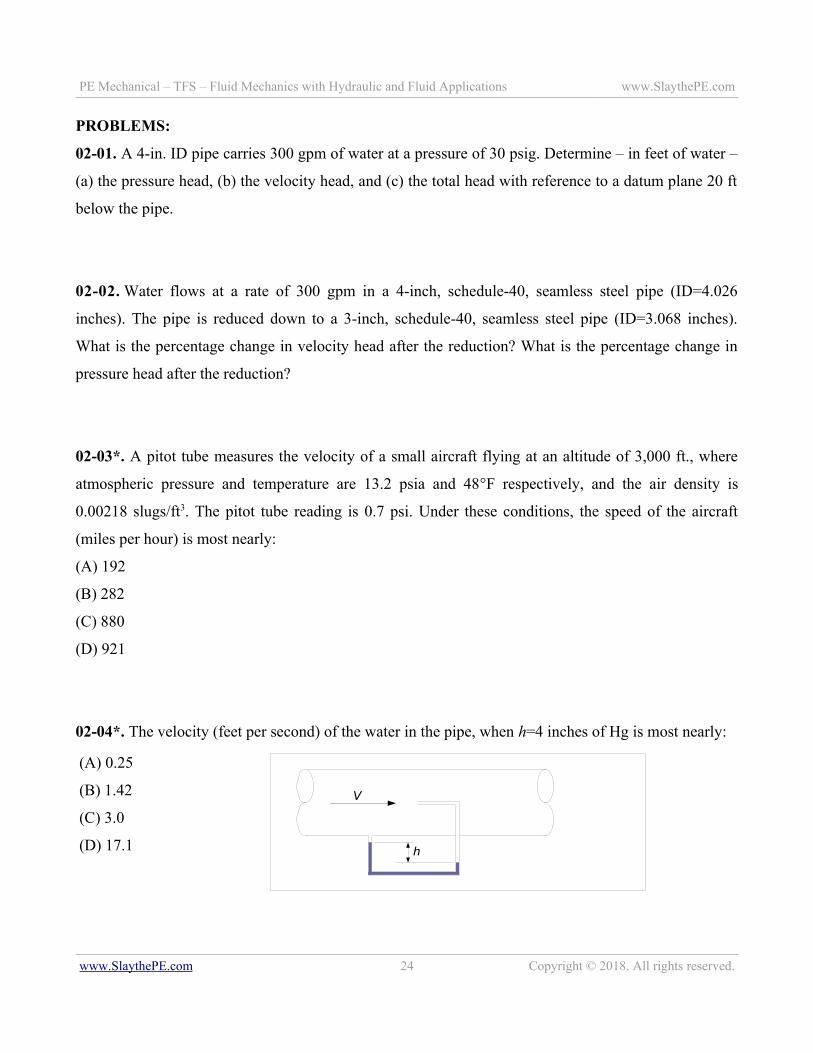
02-05*. Water is supplied to a house at pressure psupply while flowing at a velocity V supply . The

maximum velocity of water coming out of a faucet in the first floor is 20 ft/s. Neglect any friction

losses (e.g., assume inviscid flow). Under these conditions the maximum water velocity that would be

expected of the water (ft/s) coming out of the basement faucet is most nearly:

(A) 23

(B) 34

(C) 45

(D) 5020 ft/s

V supply , psupply

1st Floor

2nd Floor

Basement

2nd Floor

12 ft

4 ft

12 ft

4 ft

12 ft 12 ft

2 ft

02-06*. A fire hose nozzle has a diameter of 1.125 inches. According the local fire code, the nozzle

must be capable of delivering at least 250 gpm when attached to a 3-in.-diameter hose. Under these

conditions, the pressure (psig) that must be maintained just upstream of the nozzle is most nearly:

(A) 35

(B) 43

(C) 52

(D) 6,189




02-07*. Water flows steadily from a large tank, with negligible friction effects. The 4-in diameter

section of the thin wall tubing will collapse if the pressure there drops to 10 psi below atmospheric

pressure. Under these conditions, the largest allowable value of h (inches) is most nearly:

(A) 1.4

(B) 6

(C) 10

(D) 17

02-08*. Water at 60°F is being syphoned with a constant diameter hose from a large tank open to

atmosphere, where the local atmospheric pressure is 14.7 psia. More information is provided in the

picture. Neglecting all friction effects, the maximum height of the hill, H (ft ) over which the water can

be siphoned without cavitation (localized formation of water vapor bubbles in the hose due to

evaporation) occurring is most nearly:

(A) 21

(B) 28

(C) 36

(D) 44


h

4 ft

6 in diameter

4 in diameter

5 ft

15 ft

H



Section 03: Control Volume Analysis – Conservation of Mass & Energy

As engineers, our focus is typically on a device or a region in space into which a fluid enters and/or

leaves. We identify this region as a control volume. For the purposes of the P.E. Exam, the most

general form of the mass balance equation is:

dMdT

=∑i

min , i−∑j

mout , j (3-1)

That is, the rate at which the mass accumulates inside a control volume, dM /dT , is equal to total rate

at which mass enters the control volume, Σmin ,i minus the total rate at which mass leaves the control

volume, Σ mout , j . We use the summation signs to account for multiple inlet and/or outlet ports.

When the total rates of mass into and out of the control volume are equal, there is no mass

accumulation. This is the steady-state condition:

∑i

min ,i=∑j

mout , j (Steady State) (3-2)

If there is only one inlet and one outlet in the control volume, then:

min=mout (Steady state, one inlet, one outlet) (3-3)

For incompressible fluids (liquids, or gases that do not experience significant density changes) the

above equations can all be written in terms of volume and volumetric flow rates as well.

In incompressible Fluid Mechanics (and in the kinds of problems relevant to the PE exam) the most

used form of the energy conservation equation is the so-called “extended” Bernoulli equation7. When

applied to steady, incompressible, uniform flow with one inlet (labeled “1”) and one exit (labeled “2”)

the energy equation becomes:

hP+V 1

2

2g+

p1γ +z1=hT+

V 22

2g+

p2γ +z2+hL (3-4)

where hP is known as the “pump head” (it has units of length) and is related to the amount of energy

imparted on the fluid by the pump(s) in the control volume. Similarly, hT is related to the amount of

energy extracted from the fluid by the turbine(s). It can be shown that the power requirement by a

pump with an efficiency η P is:

7 An academic might “cringe” at this name. The Bernoulli equation is actually a momentum equation (F=ma) along a streamline. The energy equation is actually a statement of the conservation of energy principle. It just so happens that forthe particular set of problems considered here, the two reduce to similar forms.




W P=m g hP

η P (3-5)

The numerator in equation (3-5) is the amount of energy the pump must impart on the fluid. Equation

(3-5) shows the power required by the pump is slightly larger because some energy must be used to

overcome friction and other irreversibilities within the pump.

Equation (3-5) uses the mass flow rate m , which is not really that common in practice. It is far more

common to use volumetric flow rate. Focusing now on the USCS, we define the “Water Horse Power”

(WHP) as the power (in hp) that the pump adds to the water. This is also known as hydraulic or

theoretical horsepower. The numerator in equation (3-5) is the water horsepower. In terms of

volumetric flow rate, WHP can be calculated as:

WHP= h ⟨ft ⟩Q ⟨gpm ⟩SG3956

(3-6)

Equation (3-6) only works if the flow rate is in gpm and the pump head is in ft. Another useful form of

the WHP equation is:

WHP=Δ ppump⟨ psi ⟩Q ⟨gpm ⟩

1714 (3-7)

which can be used to calculate WHP if the pressure rise (in psi) across the pump is known as well as

the flow rate (in gpm) through the pump. Equation (3-7) is obtained under the assumption that the

change in velocity head across the pump is negligibly small when compared with the change in

pressure head. The WHP is the power that the pump adds to the water. The power that the motor must

deliver to the pump is the brake horse power (BHP), also known as the shaft horse power. The BHP

is slightly larger than the WHP because some energy must be used to overcome friction and other

irreversibilities. Therefore, for pumps:

BHPP=WHPη P

(3-8)

Similarly, the shaft horsepower developed by a turbine of efficiency η T is:

BHPT= ηT WHP (3-9)

where the turbine water horsepower is also calculated with equation (3-6).

The last term of equation (3-4) is the head loss, hL . This is an umbrella term that covers the effects of

viscosity-caused internal friction with its resulting temperature changes and heat transfer, as well as




energy that must be expended to sustain secondary flow patterns that are created with geometry

changes (elbows, tees, valves, etc). In pipe or conduit flow, the losses due to viscous effects are

distributed over the entire length (these are known as friction losses), whereas the loss due to a

geometry change is concentrated in the vicinity of the geometry change (these are known as minor

losses). That is, hL=hminor+h friction . The analytical calculation of these losses is quite complicated and

instead we generally rely on empirical formulas to predict them. One common approach to estimate

minor losses is to write the head loss in terms of a head loss coefficient, K so that:

hminor=(∑ K ) V 2

2 g(3-10)

In other words, the head loss is proportional to the velocity head, and the constant of proportionality is

the sum of all the loss coefficients in the system. The head loss coefficient (as well as other aspects of

the calculation of head losses such as friction losses) will be discussed in greater detail in further

sections of this book.

“Time-saving” forms of common equations:

The formal definition of water horsepower was equation (3-5), but in problem-solving situations

equations (3-6) and (3-7) are real “time-saver” alternatives because they are written in terms of

commonly used quantities such as flow rate in gpm and pressure change in psi. This approach can be

applied to many of the equations in this chapter to obtain these short-cut type equations. EXTREME

CAUTION should be applied, however, and make absolutely sure you are using the units required to

make the equations accurate:

hV =0.0155V 2=0.00259(gpm )2

D4 [hV ]=ft ; [V ]=ft s

; [ D ]=in (3-11)

Equation (3-11) quickly provides hV when the flow rate is known in gpm and the pipe ID is known in

inches. This is useful because head losses are calculated as a loss coefficient times hV .

To obtain flow velocity, given flow rate in gpm, use:

V =0.4085gpm

D2 [V ]=ft s

; [ D ]=in (3-12)

Head and pressure are used interchangeably provided that they are expressed in their appropriate units.

To convert from one to other use any of these four equations:




Liquid Head in feet=psi×2.31SG

(3-13)

Liquid Head in feet=psi×144γ [ γ ]=

lbf ft3

(3-14)

Pressure in psi=Head in ft× γ

144[ γ ]=

lbf

ft3 (3-15)

Pressure in psi=Head in ft×SG2.31

(3-16)

For water, it is typical to use γ =62.4 lbf /ft3 – which corresponds to 60°F – in Equations (3-14) and

(3-15). Also, Equations (3-13) and (3-16) show that a column of 60°F water 2.31 feet high will exert a

pressure of 1 psi at its base.

PROBLEMS

03-01. Water flows at a rate of 400 gpm in a 4-in ID pipe. The pipe enters a tee from which a 2-in ID

and a 3-in ID pipe come out. The flow velocity in the 3-in ID pipe is 8.7 feet per second. Calculate:

(a) the velocity head in the 4-in pipe upstream of the tee.

(b) the flow rate in gpm in the 3-in pipe downstream of the tee.

(c) the flow rate in gpm in the 2-in pipe downstream of the tee.

03-02. A certain valve in a 3-in pipe with 50 gpm of water causes a 1.0 psi pressure drop across the

valve. Calculate:

(a) the head loss for the valve, in feet.

(b) the velocity head, in feet.

(c) the loss coefficient for the valve.

Now, assume the loss coefficient remains unchanged when the valve is placed in a 3-in pipe carrying

175 gpm of a heat transfer fluid with SG=0.75 – what pressure drop (in psi) will occur across the valve

now?




03-03. A stream of water in a 6-in ID pipe feeds a shell-and-tube heat exchanger characterized by a loss

coefficient of K =20 . The pressure drop across the heat exchanger is not to exceed 10 psi. What is the

highest allowable flow rate (in gpm) to the heat exchanger?

03-04*. Water flows at a rate of 120 gpm in a seamless steel schedule 40, 2-in pipe (ID = 2.067 in).

The static pressure is 10 psi just upstream of an expansion to 3-in pipe (ID = 3.068 in). If the loss

coefficient associated with the expansion (based on the upstream velocity) is 0.37, the pressure (psi)

just downstream of the expansion is most nearly:

(A) 10.4

(B) 15.8

(C) 23.8

(D) 71.71

2

03-05*. Water is transported from one atmospheric pressure reservoir with surface elevation of 440 feet

to a lower atmospheric pressure reservoir with surface elevation of 80 feet through a 10-inch ID pipe.

The flow rate is known to be 7,500 gallons per minute. Under these conditions, the total loss coefficient

between the surfaces is most nearly:

(A) 15

(B) 25

(C) 30

(D) 45




03-06*. A pump with an efficiency of 85% raises the pressure of 80 gpm of water by 100 psi. The pipe

at the pump suction has a diameter of 2 inches and the pipe at the pump discharge has a diameter of 4

inches. Under these conditions, the brake horsepower for the pump is most nearly:

(A) 3.0

(B) 3.5

(C) 4.7

(D) 5.5

03-07*. The water pump shown has a brake horsepower of 30 hp and an efficiency of 90%. The flow

rate is 790 gallons per minute and all piping on the suction line is 4-in ID pipe while the short discharge

pipe is 2-in ID. The only significant head loss downstream of the pressure gage occurs across the filter.

Under the conditions shown, the head loss (ft) associated with the filter is most nearly:

(A) 34

(B) 41

(C) 130

(D) 135 open discharge

3 psi vacuum

filterPump

2”

4”




03-08*. Water at 60 psia flowing at a rate of 67,325 gallons per minute enters a hydraulic turbine

through a 3-ft ID inlet pipe as indicated in the figure. The turbine discharge pipe has a 4-ft ID. The

static pressure at section 2 (10 feet below the turbine inlet) is 10 in. Hg vacuum. The turbine has an

efficiency of 85% and develops 2.25 MW at the shaft. The head loss (ft) between sections 1 and 2 is

most nearly:

(A) 1.5

(B) 2.4

(C) 14

(D) 47

(2)

10 inHg vacuum

Turbine

4' ID

3' ID60 psia67,325 gpm

(1)

10'

03-09*. A small river with a reliable flow rate of 15.25 million cubic feet per day feeds the reservoir

shown in the figure. The turbine has a mechanical efficiency of 80% and the overall loss coefficient for

the entire system is 4.5. Under these conditions, the power developed at the shaft, in kW is most nearly:

(A) 488

(B) 588

(C) 688

(D) 78866 ft

4 ft Ø

T




03-10*. The overall loss coefficient up to point A is 3.2; from B to C, the overall loss coefficient is 1.5,

and the losses through the exit nozzle are negligible The figure shows additional information. Under

these conditions, the power requirement (hp) for the 85% efficient pump is most nearly:

(A) 3.0

(B) 3.5

(C) 4.1

(D) 4.8


50 ft 60 psig1.5 in ID

P

2 in ID

0.75 in ID

A B C

water





Documents

MECHANICAL ENGINEERING THERMAL AND FLUID SYSTEMS … · PE Mechanical – TFS – Fluid Mechanics with Hydraulic and Fluid Applications SECTION 01: Basic Information and Properties