Measuring with pressure sensitive paint in time-varying …kth.diva-portal.org/smash/get/diva2:740366/SUMMARY01.pdf · Measuring with pressure sensitive paint in time ... Increasingly

Measuring with pressure sensitive paint in

time-varying flows

by

Markus Pastuhoff

August 2014Technical Reports from

Royal Institute of TechnologyKTH Mechanics

SE-100 44 Stockholm, Sweden

Akademisk avhandling som med tillstand av Kungliga Tekniska Hogskolan iStockholm framlagges till offentlig granskning for avlaggande av teknologiedoktorssexamen den 26 september 2014 kl 14.15 i sal F3, Lindstedtsvgen 26,Kungliga Tekniska Hogskolan, Stockholm.

ISBN: 978-91-7595-246-8TRITA-MEK: 2014.18ISSN: 0348-467XISNR: KTH/MEK/TR-14/18-SE

©Markus Pastuhoff 2014

Universitetsservice US–AB, Stockholm 2014

Markus Pastuhoff 2014Measuring with pressure sensitive paint in time-varying flows

CCGEx, KTH Mechanics, SE–100 44 Stockholm, Sweden

Abstract

Increasingly tougher legislation on internal combustion engine emissions drivesthe development towards smaller engines with higher efficiency where an im-portant component is the gas-exchange system and especially the turbocharger.The flow in the gas-exchange system is inherently pulsating and unsteady andthe present thesis aims at investigating if and how pressure sensitive paint(PSP) can be used for internal unsteady flows of relevance for engine applica-tions. PSP is an optical non-intrusive technique for pressure measurements onsurfaces and in the thesis different acquisition, evaluation and signal-to-noise-raising methods have been evaluated and developed with focus on unsteadyinternal flow. In particular it describes a path towards measurements of un-steady pressure distributions on the impeller blades of turbocharger compres-sors appearing in compressors at surge.

As a first step, dynamic calibration of a polymer/ceramic pressure sensitivepaint (PC-PSP) was made using a shock tube. The cut-off frequency for thetested ruthenium-based formulation was found to be a few kilohertz; sufficientfor resolving unsteady compressor behaviour such as surge and rotating stall.

The same PC-PSP was used for measurements of the pressure on the insidewall of a y-junction sized to resemble the exhaust manifold of a car engine. Theintensity method was used where a LED array provided excitation light andluminescent intensities was acquired using a CCD camera. Phase averagingwas made in-camera by summing the intensity from several LED flashes phaselocked to the flow pulses.

A filtering technique based on singular value decomposition (SVD) wasalso developed. As a test case the fluctuating pressure field due to unsteadyvortex shedding on the side of a square cylinder was evaluated. The data wascaptured using a high speed CMOS camera and continuous LED light. Theresult was a reduction of pixel noise on the order of two magnitudes that madeit possible to recover vortex shedding behaviour otherwise submerged in noise.

Due to complex geometries and high rotational speeds, pressure measure-ments on the impeller blades are unfeasible using traditional pressure taps andtransducers and here the pressure was measured with PSP on the impellerblades of a rotating compressor. For this study, point measurements using ascanning laser for excitation and a photomultiplier tube for the acquisition ofthe luminescence was used and evaluated with the so called lifetime method.The measurements were able to capture the surge frequency as well as its spa-tial distribution.

Descriptors: Pressure sensitive paint, fluid mechanics, internal flow, pulsatingflow.

iii

Markus Pastuhoff 2014Measuring with pressure sensitive paint in time-varying flows

CCGEx, KTH Mechanics, SE–100 44 Stockholm, Sweden

Sammanfattning

Okande lagkrav pa forbranningsmotorns avgasemissioner driver utvecklingenmot motorer med hogre energieffektivitet. En viktig del i denna utvecklingar gasvaxlingssystemet och speciellt turboaggregatet. Stromningen i dessa arpulserande och instationar och malet med avhandlingen ar att undersoka omoch hur tryckkanslig farg (Pressure sensitive paint, PSP) kan anvandas i dennautveckling. PSP ar en optisk metod for att bestamma trycket pa ytor ocholika insamlings, utvarderings och signal-till-brus forbattrande metoder hari detta arbete utvecklats och utvarderats for instationar stromning. Specielltbeskrivs en metod for matningar av det trycket pa ett turboaggregats roterandekompressorblad.

Som ett forsta steg har frekvenskarakteristiken hos s.k. “polymer/ceramic”tryckkanslig farg (PC-PSP) uppmatts med hjalp av ett stotror. Responsen hosden ruthenium-baserad fargen nar upp till ett par kHz vilket ar tillrackligt foratt mata trycken vid de instationara kompressorfenomenen surge och roterandestall.

Samma tryckkansliga farg anvandes ocksa for matning av vaggtrycket vidpulserande stromning i en y-kanal liknande grenroret hos en bilmotor. In-tensitetsmetoden anvandes med ett antal LED lampor som exciterade fargenoch luminiscensen registrerades med en CCD kamera. Fasmedelvardesbildninggjordes direkt i kameran genom att summera intensiteten vid flera LED pulserfaslasta till stromningen.

En filterteknik baserad pa singularvardesuppdelning har ocksa utvecklats.Som ett testfall har det fluktuerande tryckfaltet som uppkommer vid insta-tionar virvelavlosning pa en sida av en kvadratisk cylinder utvarderats. Lu-miniscensen registrerades med en CMOS hoghastighetskamera vid kontinuerligLED belysning. Filtreringstekniken minskade pixelbruset med tva storleksor-dningar och gjorde det mojligt att studera virvelavlosningsstrukturerna, vilkai den ursprungliga signalen var helt drankta i bruset.

Pa grund av komplex geometri och hoga rotationshastigheter ar det svart,for att inte saga omojligt, att mata trycket pa kompressorbladen med konven-tionella tryckhal och tryckgivare och istallet bestamdes trycket med hjalp avPSP. En laserstale som svepte over bladen gjorde punktvisa matningar mojligaoch en fotomultiplikator registrerade luminiscensen. Intensiteten utvarderadessedan med den s.k. livstidsmetoden. Genom matningarna kunde “surge-frekvensen” och tryckets spatiella struktur bestammas.

Descriptors: Tryckkanslig farg, stromningsmekanik, internstromning, pulserandestromning.

iv

Part of this work have been presented at the

following conferences:

7th

International Conference on Flow Dynamics,1–3 November 2010, Sendai, Japan

6th

Interdisciplinary Forum on Molecular Imaging,8 November 2010, Tokyo, Japan

Svenska Mekanikdagar,13–15 June 2011, Chalmers Goteborg, Sweden

10th

International Symposium on Experimental and Com-

putational Aerothermodynamics of Internal Flows,4–7 July 2011, Brussels, Belgium

9th

International Conference on Flow Dynamics,19–21 September 2012, Sendai, Japan

66th

Annual Meeting of the APS Division of Fluid Dy-

namics,24–26 November 2013, Pittsburgh, PA, USA

v

vi

Contents

Abstract iii

Sammanfattning iv

Part I. Overview and summary

Chapter 1. Introduction 3

1.1. Conventional pressure measurements 4

1.2. The ideal gas law and properties of air 5

1.3. Some pressure relations 6

1.4. Pressure variation across boundary layers 8

1.5. Some relevant conditions for internal combustion engines 8

1.6. Layout of the thesis 8

Chapter 2. Basic Physics of PSP 10

2.1. A historical note – the detection of photoluminescence 10

2.2. The quantum mechanics behind photoluminescence – the Jablonksidiagram 11

2.3. Quantum yield, quenching and life time 12

2.3.1. Stern-Volmer equation 12

2.3.2. Intensity method 13

2.3.3. Lifetime method 13

2.4. Paint preparation for steady and unsteady conditions 15

2.5. Previous experiments 17

Chapter 3. Experimental flow set ups 21

3.1. Time response determination 21

3.1.1. Shock tube and experimental technique 21

3.1.2. Results for PC-PSP time response 22

3.2. Pulsating flow in a y-junction 23

vii

3.2.1. Pulsating rig and experimental y-junction set-up 23

3.3. Vortex shedding from a cylinder 24

3.3.1. Wind tunnel, cylinder and experimental technique 25

3.4. Compressor flow 26

3.4.1. Compressor test-flow facility 26

Chapter 4. Applications of PSP 29

4.1. Paint calibration 29

4.1.1. In situ calibration 30

4.2. Instrumentation and methods for data acquisition 32

4.2.1. Intensity imaging 32

4.2.2. An alternative to wind-off images for pulsating flows 33

4.2.3. Scanning laser measurements 33

4.3. A note on temperature errors 36

4.4. Noise reduction techniques 37

4.4.1. Temporal and spatial low-pass filtering 37

4.4.2. Phase averaging 38

4.4.3. Singular value decomposition for noise reduction 40

Chapter 5. Summary of results and main conclusions 43

Chapter 6. Papers and authors contributions 46

Acknowledgements 49

References 50

Part II. Papers

Paper 1. Dynamic calibration of polymer/ceramic pressure

sensitive paint using a shock tube 59

Paper 2. Wall pressure measurements in a y-junction at pulsating

flow using polymer/ceramic pressure sensitive paint 67

Paper 3. Enhancing signal-to-noise ratio of pressure sensitive

paint data by singular value decomposition 81

Paper 4. Pressure sensitive paint measurements on a turbocharger

compressor 101

viii

Part I

Overview and summary

CHAPTER 1

Introduction

Increasingly tougher legislation on internal combustion engine emissions drivesthe development towards smaller engines with higher efficiency where an im-portant component is the gas-exchange system and especially the turbocharger.The flow in the gas-exchange system is inherently pulsating and unsteady andthe present thesis aims at investigating if and how pressure sensitive paint(PSP) can be used for internal unsteady flows of relevance for engine applica-tions.

Pressure is, from an engineering point of view, maybe the most importantfluid dynamic quantity, since it is through the pressure the main forces fromthe fluid are transferred to the engineering component such as a wind-turbineblade or engine piston, or the opposite, how mechanical energy is transferred toa fluid in e.g. a compressor or a pump. Pressure differences are also the drivingforce of flow in pipe lines and other conduits. The pressure force dF acting onthe small surface element dS (may it be a solid wall or a virtual surface insidethe fluid) is

dF = −pndS

where p is the pressure which is a positive scalar and n is the normal vectordirected outward from the surface, hence defined as being normal to the surface.In a gas the origin of the pressure can be viewed as the exchange of momentumof gas molecules that are colliding with the surface. There are of course alsoforces tangential to the surface, so called viscous forces, and the shear stress atthe wall is defined as

τw = µw

�dU

dn

�

w

eτw

where µw is the dynamic viscosity at the wall, and (dU/dn)w the velocitygradient at the wall. The viscous forces are typically much smaller than thepressure forces but can still be of high importance, for instance they may becrucial when it comes to the drag on a body moving through a fluid.

In the following we will discuss pressure measurements in air and gas flows.This does not mean that pressure measurements in liquids (such as pressuredrop in pipe lines or blood pressure) are of less interest but these are not thefoci of the present theses.

3

4 1. INTRODUCTION

1.1. Conventional pressure measurements

Barometric pressure is measured in order to foresee the weather, blood pres-sure in order to assess our health, and car-tyre pressure in order to keep gasconsumption and tyre wear to a minimum to mention a few examples wherepressure is sought in itself. We also use pressure as an information carrier,an example is sound where we measure pressure variations using microphones.However, here we are usually not as interested in acquiring the pressure as weare in the speech or music contained within the signal. Another example isthe use of barometers as altimeters utilizing the fact that atmospheric pressuredecreases with height over sea level.

Pressure measurements have a long history and the oldest device is thebarometer to measure air pressure. The invention of the barometer is usuallyascribed to the Italian scientist Evangelista Torricelli (1608–1647) who around1643 filled a roughly 1 m long glass test tube with mercury and submerged theopen end in a basin of mercury, whereupon the mercury column inside the tubefell, leaving a vacuum above. Torricelli doubted the common belief that themercury column was pulled up by the attractive power of vacuum. He insteadspeculated that air had mass and that the pressure balanced the force from theweight of the mercury, or in his own famous words:

“We live submerged at the bottom of an ocean of air.”

For a more extensive treatment on the contributions of Torricelli, the reader isrefereed to Middleton (1963).

A differential manometer, the so called U-tube manometer, where the dif-ference in height between the two liquid columns is proportional to the pressuredifference was invented by Christiaan Huygens in 1661. The French hydraulicengineer Henri Pitot realized that he could measure velocities by inserting anopen tube with opening facing the flow and measured the velocity distributionof the water movement in the river Seine around 1732, and was able to showthat the velocity did not increase with depth which was the common belief atthe time.

Today the liquid manometers are usually replaced by pressure sensorswhere the pressure difference between the two sides of a thin flexible mem-brane makes it deflect. The deflection can be mechanically transferred to ameter needle, or converted into an electric signal in which case the device isa pressure transducer. Conversion into an electrical signal can be done in nu-merous ways, of which perhaps the most common is to attach strain gauges tothe membrane. In this way the deflection can be converted into a change inresistance which in turn can be converted to a voltage change with the use ofa Whetstone bridge. The membrane deflection can also be measured opticallyby observing the interference pattern of monochromatic light mirrored of themembrane.

1.2. THE IDEAL GAS LAW AND PROPERTIES OF AIR 5

A different type of sensors are the piezo-crystal based pressure transducers.These sensors are not based on the deflection of a membrane, but rather on thechange of physical properties the material undergo under compression. Thepiezo-resistive type utilizes the relation between compression and resistanceof the material and the piezo-electric type measures the charge induced uponcompression. An example is the spark produced in an electric lighter, generatedby striking a piezo crystal.

Yet another method to measure the pressure in gases is the Pirani methodwhich is based on the heat transfer from an object which in turn depends onthe density and therefore pressure of the gas.

Today pressure measurements is a standard technique in any areas of sci-ence and technology, such as the determination of pressure distributions onmodels of aircraft and other objects in wind-tunnel experiments. Another.most important technological system is the internal combustion engine whichis equipped with several pressure sensors for diagnostic purposes or used forinputs to the engine control system. An example of the first kind is pressure-difference measurements across the particle filter in order to determine when itstarts to become clogged. Other systems are used to measure flow rates in thegas-exchange system. In engine flows the pressure is typically non-stationaryor rather pulsating which makes accurate measurements more complicated ascompared to steady flows.

However fascinating the subject of mechanical pressure sensors, this thesisutilizes a completely different method that is based on the determination ofthe partial pressure of oxygen through its extension of photoluminescence insome substances. For air in chemical equilibrium, the concentration of oxygenis given and the partial pressure is directly proportional to the pressure. Themethod is usually called PSP or “Pressure Sensitive Paint”, and since it is apaint one realizes that is applied on solid surfaces, although there have beensome attempts to use the same method on particles that are following the flowfield. In the following parts of this chapter some basics of gases and pressuremeasurements are given.

1.2. The ideal gas law and properties of air

In many cases a gas can viewed as ideal, which means that intermolecular forcescan be neglected. Deviations from ideal behaviour occur at high pressuresand/or low temperatures, but for the present work where the conditions areclose to STP1, the gas can be considered as ideal.

The ideal gas law is given as

pV = nRT

1STP refers to Standard Temperature and Pressure, corresponding to a temperature of 273 Kand a pressure of 100 kPa

6 1. INTRODUCTION

Constituent Fraction Molecular weight[%] kg/kmol

N2 78.1 28.02O2 20.9 32.00Ar 0.9 39.94CO2 0.03 44.01other < 0.07 -air 100 28.97

Table 1.1. Main constituents of dry air at STP.

where V is the volume of the gas, n the number of moles and R the universalgas constant. The value of R is 8.314 J/K mol. For a given gas mixture thespecific gas constant is R = R/M where M is the weight of one mole of thegas molecules in the mixture. Using the specific gas constant instead the idealgas law can be written

pv = RT

where v is the specific volume; v = ρ−1, and ρ is the density of the gas. Thisequation can be seen as an equation of state for the gas.

Air is a gas consisting of many different constituents and its compositionalso depends on the temperature since various types of reactions may occurdepending on the temperature. For dry air (i.e. air without water vapor) atSTP the main constituents can be found in Table 1.1 and the correspondingweight of one mole of air is Mair = 28.97 · 10−3 kg, giving the value of Rair =286.9 J/kg K.

The pressure exerted by a gas on its surroundings is given by the partialpressure of the different constituents which is known as Dalton’s law. For airwe could write

pair = pN2 + pO2 + pAr + pCO2 + pother.

The partial pressure of a constituent (pi) can be calculated as

pi = xip

where xi is the mole fraction of the constituent. Inversely, if the partial pressureof a constituent is known as well as its mole fraction, then the pressure of themixture can be calculated as

p = pi/xi.

This means that as long as the mole fraction stays constant pi/p =constant.

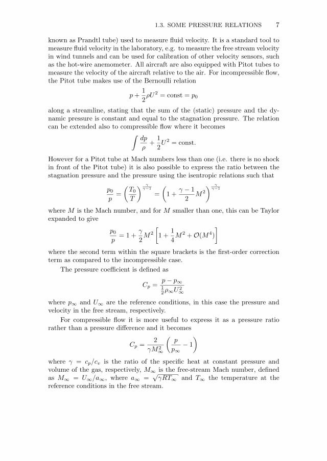
1.3. Some pressure relations

Pressure measurements are used in many situations, maybe one of the mostwell known application is the Pitot tube or Pitot-static pressure tube (also

1.3. SOME PRESSURE RELATIONS 7

known as Prandtl tube) used to measure fluid velocity. It is a standard tool tomeasure fluid velocity in the laboratory, e.g. to measure the free stream velocityin wind tunnels and can be used for calibration of other velocity sensors, suchas the hot-wire anemometer. All aircraft are also equipped with Pitot tubes tomeasure the velocity of the aircraft relative to the air. For incompressible flow,the Pitot tube makes use of the Bernoulli relation

p+1

2ρU2 = const = p0

along a streamline, stating that the sum of the (static) pressure and the dy-namic pressure is constant and equal to the stagnation pressure. The relationcan be extended also to compressible flow where it becomes

�dp

ρ+

1

2U

2 = const.

However for a Pitot tube at Mach numbers less than one (i.e. there is no shockin front of the Pitot tube) it is also possible to express the ratio between thestagnation pressure and the pressure using the isentropic relations such that

p0

p=

�T0

T

� γγ−1

=

�1 +

γ − 1

2M

2

� γγ−1

where M is the Mach number, and for M smaller than one, this can be Taylorexpanded to give

p0

p= 1 +

γ

2M

2

�1 +

1

4M

2 +O(M4)

�

where the second term within the square brackets is the first-order correctionterm as compared to the incompressible case.

The pressure coefficient is defined as

Cp =p− p∞1

2ρ∞U2

∞

where p∞ and U∞ are the reference conditions, in this case the pressure andvelocity in the free stream, respectively.

For compressible flow it is more useful to express it as a pressure ratiorather than a pressure difference and it becomes

Cp =2

γM2∞

�p

p∞− 1

�

where γ = cp/cv is the ratio of the specific heat at constant pressure andvolume of the gas, respectively, M∞ is the free-stream Mach number, definedas M∞ = U∞/a∞, where a∞ =

√γRT∞ and T∞ the temperature at the

reference conditions in the free stream.

8 1. INTRODUCTION

1.4. Pressure variation across boundary layers

A most important observation is that for thin boundary layers, which is typi-cally the case for attached boundary layers (i.e. non-separating), the pressureat the body surface is the same as in the free stream. From the case of a two-dimensional laminar boundary layer one immediately finds that the pressure isconstant across the boundary layer, i.e. pw = p∞. For a turbulent boundarylayer one finds that

p+ ρ < v2>= pw

where < · > denotes a time (or ensemble) average and v is the fluctuatingvelocity component normal to the surface. However since < v2 > vanishes alsoin the free stream one finds that pw = p∞, i.e. the wall pressure is the sameas the free-stream pressure also in a turbulent boundary layer. On the otherhand inside the turbulent boundary layer the static pressure varies and we canwrite

p− pw1

2ρU2

= −ρ < v2 >

1

2ρU2

= −2< v2 >

U2= −2

< v2 >

u2τ

u2τ

U2

The maximum relative deviation of the local static pressure as compared tothe static pressure at the wall can be estimated to be around 1% for a turbu-lent boundary layer as well as for channel and pipe flows, giving errors of theestimated velocity around 0.5% if the static pressure is measured by a pressuretap at the wall rather inside the flow itself.

1.5. Some relevant conditions for internal combustion engines

Flow in internal combustion engines are by its nature pulsative with frequenciesin the order of 102 Hz, excluding the turbocharger region where the bladepassage frequency can exceed this by order of two magnitudes. Measuringthe pressure on the blades, or in their proximity, of a compressor rotating at200 000 rpm with a radial resolution of 1 degree would require a system fastenough to resolve 1.2 MHz.

Pressure sensitive paint (PSP) has shown to be a promising technique inorder to overcome the issue of difficult probing. However, the response timesof traditional paints are orders of magnitude to slow to resolve all temporalbehaviour in turbocharger applications.

1.6. Layout of the thesis

This thesis deals with measurements of pressure with so called pressure sensitivepaint (PSP), mainly in non-steady cases. i.e. when the flow is unsteady dueto forced pulsations or dynamics inherent in the flow motion itself. The formerrefers to pulsating flows in complex channels, the latter refers to vortex sheddingfrom a cylinder or pulsations during compressor surge.

Chapter 2 describes the theory and practice of the PSP technique withreferences to the literature, both for steady and time-resolved measurements.

1.6. LAYOUT OF THE THESIS 9

Chapter 3 describes the experimental setups used, whereas chapter 4 gives sometheoretical background for the evaluation techniques and these are exemplifiedby the different studies in the thesis. Chapter 5 is a brief summary of the papersappended to the thesis, followed by the acknowledgment and a reference list.

CHAPTER 2

Basic Physics of PSP

The technique for obtaining pressure measurements using pressure sensitivepaint is based on the photoluminescence and oxygen quenching of certainmolecules, or luminophores. In short one may say that these molecules, whenexposed to light of a certain wavelength, become luminous, i.e. they emit lightat a longer wave length. However the intensity and the time history of the emit-ted light depends on several factors and for the luminophores used for PSP theamount of oxygen in contact with the material is one such factor. With in-creasing amount of oxygen the intensity of the emitted light decreases as wellas the decay time of the luminescence, so called oxygen quenching. Since theamount of oxygen is directly coupled to the partial pressure of oxygen, andtherefore also to the pressure in the air itself the luminescence can be used todetermine the air pressure.

In this chapter we give a background on the chemistry/physics of lu-minophores, as well as some practical details of the technique that have beenused in the present work in order to prepare the surface for PSP. We have alsomade a collection of earlier work on PSP, however we do not intend a thoroughreview of earlier work since for the interesting reader there exist several recentexcellent review articles of the use of PSP, such as Liu et al. (1997a); Bellet al. (2001); Gregory et al. (2008, 2014) as well as a textbook; Liu & Sullivan(2005). One may note from the literature presented that most published workstill deals with the technique itself and there are so far only few fluid dynamicsquantitative results.

2.1. A historical note – the detection of photoluminescence

It has been known for centuries that certain compounds emit light under expo-sure from the sun. As early as 1565 a Spanish physician and botanist, NicholasMonardes, reported that water containing a certain kind of wood, then knownas lignum nephriticum, would glow with a blue tint when exposed to sunlight.Also Boyle (1664) made some remarks about this in his monograph on colours.

Minor progress was made in 1845, observing a solution of quinine sulfateexposed to sunlight, Sir John Frederick William Herschel (1792 – 1871) re-ported:

10

2.2. THE QUANTUM MECHANICS BEHIND PHOTOLUMINESCENCE 11

“Though perfectly transparent and colourless when held betweenthe eye and the light, or a white object, it yet exhibit in certainaspects, and under certain incidences of the light, an extremelyvivid and beautiful celestial blue colour [...]”

and in 1852 Sir George Gabriel Stokes (1819 – 1903) expanded on Herschel’sexperiment with the addition of different excitation and emission filters. Byfiltering the sunlight through a blue stained glass window and observing thesolution through a glass of yellow wine, Stokes discovered that fluorescent emis-sion occurs at longer wavelengths than excitation, what we today call Stokesshift. However, neither Herschel nor Stokes could explain the phenomena us-ing the scientific knowledge of their time since the explanation is of quantummechanical origin.

2.2. The quantum mechanics behind photoluminescence – the

Jablonksi diagram

The possible energy states of a luminophore can be described by a Jablonski1

energy-level diagram as shown in figure 2.1, where the lowest horizontal linerepresents the ground state of the molecule. For a majority of molecules theground state is a singlet state, indicating that the sum of quantum spin is equalto 0. The singlet states are depicted by Si where the index i denotes differentelectron energy levels. Furthermore, within each electron energy level thereexist a number of vibrational levels (depicted by 0, 1 and 2 in the S0 state).

S0

Absorption

hνa210

S1

S2

Internal conversion

hνa

Fluorescence

hνf

T1

Intersystem crossing

Phosphorescencehνp

Figure 2.1. Jablonski energy-level diagram

With the absorption of a photon with a proper energy quantum, the lu-minophore is excited to a higher energy singlet state, S0 + hνa → S1 or

1From Polish physicist Aleksander Jab�lonski (1898–1980)

12 2. BASIC PHYSICS OF PSP

S0 + hνa → Sn where h is the Planck constant and νa is the frequency ofthe absorbed photon.2

The excited electrons can now return to the ground state via a number ofradiative and non-radiative paths. Relaxation between the vibrational stateswithin the electron energy level, as well as relaxation to a lower level, suchas S2 → S1, are called internal conversion. Electrons in the higher singletstates can also undergo spin-conversion to the triplet states (where the sum ofquantum spin is equal to 1). Both these processes are non-radiative.

Fluorescence (depicted by hνf ) occurs when electrons return to the electronground state by S1 → S0 + hνf and phosphorescence (hνp) by T1 → S0 + hνp.The two phenomena are jointly called luminescence, and when the electronsare initially excited by light; photoluminescence.

2.3. Quantum yield, quenching and life time

As seen in figure 2.1, not all paths to the S0 state lead to luminescent emissions.Decreases in luminescent intensity are called quenching and can occur due toa number of sources, of which thermal quenching and collisional quenching byoxygen are the most important ones in a pressure sensitive paint context.

2.3.1. Stern-Volmer equation

If we let kr denote the emissive rate of luminescence, kq[O2] the rate of oxygenquenching (where [O2] is oxygen concentration) and knr the rate of all othernon-radiative decays to S0, the quantum yield can be defined as

Φ =kr

kr + kq[O2] + knr(2.1)

or, with I as luminescent intensity and Ia as absorption,

Φ =I

Ia. (2.2)

Without quenching the quantum yield becomes

Φ0 =I0

Ia=

kr

kr + knr(2.3)

with I0 denoting luminescent intensity in the absence of quenching. DividingΦ0 by Φ yields

Φ0

Φ=

I0

I= 1 +

kq

kr + knr[O2] (2.4)

Luminescent lifetime is defined by the average time a molecule spends inan excited state;

τ =1

kr + kq[O2] + knr(2.5)

2The energy of the photon and its frequency are related through what is known as thePlank-Einstein relation, E = hν, where the Planck constant h = 6.62606957 · 1034 Js.

2.3. QUANTUM YIELD, QUENCHING AND LIFE TIME 13

and without quenching τ0 = 1/(kr + knr). Insertion into eqn. (2.4) gives theStern-Volmer equation

I0

I=

τ0τ

= 1 +K[O2] (2.6)

where K = kqτ0 is the Stern-Volmer quenching constant.

2.3.2. Intensity method

The use of PSP builds on Henry’s law, which states that the amount of a givengas that dissolves in a material is directly proportional to the partial pressureat a given temperature, together with Dalton’s law, stating that the pressure, pof a gas equals the sum of the partial pressures of the species therein. Under theassumption that the molecular concentration of oxygen is constant, i.e. thereare no chemical reactions, the Stern-Volmer equation can be rewritten as

I0

I= 1 +Kp (2.7)

In practical applications I0 (at p = 0) may be difficult to obtain andtherefore a reference pressure pref with corresponding reference luminescentintensity Iref is used such that

I0

Iref= 1 +Kpref . (2.8)

Division by eqn. 2.7 gives

Iref

I=

1 +Kp

1 +Kpref=

1

1 +Kpref+

Kpref

1 +Kpref

p

pref(2.9)

and finally, setting A = (1+Kpref )−1 and B = Kpref (1 +Kpref )−1 gives theform of the Stern-Volmer equation most often seen in the context of PSP,

Iref

I= A+B

p

pref. (2.10)

A and B are usually called the Stern-Volmer coefficients, and their valuedepend on the chosen reference pressure. A complication that arises is thatthey also are functions of temperature.

2.3.3. Lifetime method

A second method to evaluate the pressure is based on the time decay of theluminosity if the layer (or a point) is illuminated by a time varying source,E(t). For such a case the luminosity can be modeled as a simple first ordersystem

dI

dt= − I

τ+ E(t). (2.11)


where τ is the time constant of the luminescent decay. In practice E(t) is oftenchosen as a short duration pulse, giving a response of the luminophore thatwill show an exponential decay

I(t) = I0 exp(−t/τ). (2.12)

From Eq. 2.6 we can now also write

τrefτ

= A+Bp

pref. (2.13)

There are two different possibilities to use the lifetime method, dependingon how the response of the PSP is collected. Most studies use a camera todetect the emitted light and integrate the light over two (and sometimes three)different time intervals during the decay phase, i.e. the camera is exposed tothe light during certain non-overlapping gating periods, say t1 < t < t1 + g1

and t2 < t < t2 + g2. This gives the intensity as an integral over these periods.It is easy to show that the ratio of integrated emissions (A1 and A2) becomes

A1

A2

=e−t2/τ

e−t1/τ

(1− e−g2/τ )

(1− e−g1/τ ).

The first gate is typically short (g1 << g2) and is taken close after the pulseexcitation whereas the second is much longer and reaches to a point where theintensity has fallen close to zero. If we also assume that t2 = t1 + g1, i.e. thesecond gate opens directly when the first closes it is possible to show that

τ =g1

ln(1 +A1/A2).

If now the same procedure is done for the reference case one may write

τrefτ

=(A2/A1)ref

A2/A1

= A+Bp

pref

assuming A1 << A2. This relation is given by Gregory et al. (2014).

By instead measuring the intensity both at the reference condition and atthe condition of interest, at two specific different times (t1 and t2) after thelight impulse, we obtain for the reference condition

I1,ref = I0,ref exp(−t1/τref ) and I2,ref = I0,ref exp(−t2/τref ).

By now taking the logarithm of these equations and subtract them we obtain

τref ln

�I1,ref

I2,ref

�= t2 − t1.

We can write a similar relation for the condition of interest giving

τ ln

�I1

I2

�= t2 − t1

2.4. PAINT PREPARATION FOR STEADY AND UNSTEADY CONDITIONS 15

and now by combining them we obtain

τrefτ

=ln(I1/I2)

ln(I1,ref/I2,ref )= A+B

p

pref.

This method has been used for one of the studies in the present thesis wherethe light from the luminophore has been collected through a photo-multiplier.

2.4. Paint preparation for steady and unsteady conditions

There are several principles how to deposit the luminophore on a surface andsome of the most important ones are depicted in figure 2.2. In conventional PSPfor steady pressure measurements the luminophore is embedded in an oxygenpermeable binder. However the diffusion time is proportional to h2/α whereh is the depth into the layer and α the diffusion constant of oxygen moleculesinto the binder. The diffusion constant is of the order of 10−9 m2/s and for alayer depth of 10 µm, diffusion times are of the order of 0.1 seconds, hence thisdeposition technique is unsuitable for measurements of unsteady pressure.

For unsteady measurements two different deposition techniques that allowso called fast PSP have been developed. The first such technique was based onhaving a surface of anodized aluminum on which the luminophore was deposited(AA-PSP). The anodizing process increases the surface area substantially andallows a sufficient amount of the luminophore to be deposited directly on thesurface and hence it has direct contact with the gas. However the disadvantagewith this technique is that the surface has to be of aluminum and in order totreat the surface it has to be possible to extract part of the wall from the modelto be investigated.

A second method of these fast paint formulations, is a polymer/ceramicpressure sensitive paint (PC-PSP). The basics of PC-PSP are the same as inconventional PSP. The difference between conventional and polymer/ceramicPSP lie instead in the method of binding the luminophore to the surface.

In conventional PSP the luminophores are embedded in an oxygen perme-able binder which is then painted onto a surface. Increasing the paint layerthickness increases the emitted light intensity but decreases the frequency re-sponse resulting in a trade-off between a fast system - thin layer - and a sensitivesystem - thick layer. In PC-PSP this problem is addressed by first applying aslurry of ceramic particles in a polymer binder to the surface, thus effectivelyincreasing the surface area by making it “porous”. Luminophores are then ap-plied to the ceramic layer. Schematics of conventional, AA-PSP and PC-PSPare shown in figure 2.2.

The polymer/ceramic pressure sensitive paint used in the present workwas prepared according to a method developed by Scroggin and Gregory anddescribed by Gregory et al. (2008). The base coat was a ceramic slurry madefrom a mixture of TiO2 particles, dispersant (Rohm&Haas D-3005) and purewater at a weight ratio of 1.72:0.072:1. The slurry was ball milled for one


OxygenLuminophores

Binder

Model surface

Oxygen

Incident light, �νa

Lumines

cence,

quenching

�νf+ �νp

OxygenLuminophores

Model surface (anodized aluminum)

Oxygen


Lumines

cence,

quenching

�νf+ �νp

OxygenLuminophores

BinderModel surface

Oxygen


Lumines

cence,

quenching

�νf+ �νp

TiO2

Figure 2.2. Three different ways to prepare a PSP surfacelayer. Upper: Conventional PSP, middle: Anodized Alu-minum PSP, lower: Polymer/Ceramic PSP.

hour after which a polymer binder (Rohm&Haas B-1000) was added to themixture by a weight fraction of 3.5%. The slurry was applied to the surfaceusing a spray gun and let to dry. Two different types of luminophore were used:

2.5. PREVIOUS EXPERIMENTS 17

one ruthenium based ([Ru(phen)3]2+), and the other on platinum porphyrin(Pt-TFPP). They were both solved in methanol in ratios of 0.3 · 10−3, and0.2 · 10−11 mol/L, respectively, and was sprayed on top of the ceramic layer toform the active PSP layer.

2.5. Previous experiments

In the early 1980s studies of pressure sensitive paint began at the CentralAero-Hydrodynamic Institute (TsAGI) in Russia where the focus has beenmainly on intensity-based measurements. A number of PSP formulations weredeveloped and applied, mostly in the transonic and supersonic regimes, Bukovet al. (1994); Moshasrov et al. (1998); Troyanovsky et al. (1993).

Unaware of the work conducted behind the iron curtain, PSP was devel-oped independently by the University of Washington in collaboration with theNational Aeronautics and Space Administration (NASA) Ames Research Cen-ter and the Boeing Company in the USA. Initial research was aimed at oxygensensing for biomedical applications but the value for aerodynamic testing wassoon realized. The group developed a platinum-octaethylporphorin (PtOEP)based paint formulae and conducted measurements on a NACA 0012 airfoil atvarious air speeds; Kavandi et al. (1990) at Mach 0.3-0.66, McLachlan & Bell(1995) at Mach 0.7-0.9 and Brown et al. (1998) at Mach 0.03-0.14. This workestablished the basic experimental procedure used for intensity-based PSP mea-surements. Studies on PSP were also conducted at McDonnell Douglas (nowthe Boeing Company) where mainly ruthenium-based PSP has been used inflows ranging from low subsonic to supersonic flows, Morris (1995); Dowgwilloet al. (1996).

One of the clear advantages with PSP in comparison to other pressuremeasurement techniques is the possibility to apply the technique on rotatingcomponents without the complication to employ rotating couplings (either elec-tric or pneumatic). At Purdue University in the USA development work withfocus on rotating machinery was started already in the middle of the 90’s.,Burns & Sullivan (1995); Liu et al. (1997b); Torgerson et al. (1998); Gregory(2002, 2004).

In tables 2.1 and 2.2 a selection of papers dealing with both steady andunsteady PSP techniques, are collected. A search on Web-of-Science startingfrom 1990 reveals about 180 papers and 160 patents when searching for ”pres-sure sensitive paint” in the title. Figure 2.3 gives the numbers, and it seems tohave been a rather constant publication rate of an average of about 10 papersper year since year 2000. A general remark is that many studies deal with thedevelopment of the technique itself rather than the physics of a specific fluiddynamics setup, which is also reflected by the source of the publications, mainlyin conference proceedings, in journals focussed on measurement techniques, orin review journals.


Reference Metod CommentReview articles

Liu et al. (1997a) ReviewBell et al. (2001) ReviewAsai et al. (2001) ReviewLiu & Sullivan (2005) BookAerodynamic high speed flows

Kavandi et al. (1990) Intensity ?Troyanovsky et al. (1993) Intensity ?Bukov et al. (1994) Intensity ?McLachlan & Bell (1995) Intensity M = 0.7− 0.9Dowgwillo et al. (1996) Intensity High-speed WTMoshasrov et al. (1998) Intensity ?Shimbo et al. (2000) Intensity High speedLepicovsky & Bencic (2002) Intensity Fan cascadeMebarki & Le Sant (2001) Intensity wing M = 0.74Tillmark & Alfredsson (2004) Intensity Bump M = 0.6− 0.7Mitsuo et al. (2006) Lifetime M = 0.55− 0.6Aerodynamic low speed flows

Morris (1995) Intensity WTTorgerson et al. (1996) Lifetime/Intensity WTBrown et al. (1998); Brown (2000) Intensity WTAider et al. (2001) Intensity WT/CarLe Sant et al. (2001) Intensity WTEngler et al. (2002) Intensity WTMitsuo et al. (2002) Lifetime WTMitsuo et al. (2004) Intensity WTRotating machinery flows

Burns & Sullivan (1995) Lifetime/Intensity WTBencic (1995, 1997, 1998) Intensity WTLiu et al. (1997b) Intensity WTNavarra (1997); Navarra et al. (2001) Intensity WTSchairer et al. (1998) Intensity ?Gregory (2002, 2004) Intensity F-PSP

Table 2.1. Examples of various steady PSP studies dividedinto different application areas. “?” under “comment” in-dicates references that were unavailable to us, but has beenreferenced in review papers.

2.5. PREVIOUS EXPERIMENTS 19

Reference Method CommentReview article

Gregory et al. (2008) ReviewGregory et al. (2014) ReviewVarious applications

Nakakita et al. (2000); Nakakita & Asai (2002) Intensity M = 10Sakaue & Sullivan (2001); Sakaue et al. (2002) Intensity Shock tube test AA PSPGregory (2002, 2004) Intensity RotatingKameda et al. (2005) Intensity WTFang et al. (2011) Intensity WTGardner et al. (2014) Intensity WT

Table 2.2. Examples of various fast PSP studies.

1990 1995 2000 2005 20100

5

10

15

20

25

30

Year

Publications

Figure 2.3. Papers (◦) and patents (×) having “pressure sen-sitive paint” in the title as obtained from the ISI Web of Sci-ence starting from 1990.

The first PSP studies were made in the upper subsonic–transonic velocityregimes. In these regimes the free-stream velocities are high enough to producehigh pressure differences, while the temperature differences are still small ascompared to the supersonic regime.


As the PSP technique evolved together with improved instrumentation, re-search was pushed in the direction of lower free-stream velocities, while main-taining the focus on external flow for aerospace applications. In these areasPSP can be considered a mature measurement technique and it is applied forindustry research at a number of facilities such as those of DLR, ONERA,JAXA, NASA, Boeing etc.

Today there is also a strive towards dynamic measurements but so far theliterature is much smaller than for steady PSP. It can however be foreseen toincrease substantially since the type of measurements that can be done with fastPSP is clearly something that is more or less unavailable for other techniques.

CHAPTER 3

Experimental flow set ups

This chapter describes the four different setups and the methodology used inthe thesis. The aim from the start of the project was to establish a proofof concept for measurements of the pressure on the compressor blades of aturbocharger at high rotational speeds. This project has followed a path wherefirst the technique to mix and deposit the paint was developed and this isshortly described in section 2.4. The time response of the pressure sensitivepaint was determined through a shock-tube experiment (section 3.1) and wasfound to be of the order of a few kilohertz which was deemed sufficient for thefuture experiments. The intensity technique was explored in a pulsating flowthrough a y-junction (section 3.2). In a third study the pressure variations dueto vortex shedding on one of the sides of a square cylinder placed in a windtunnel was determined at low speeds. In order to obtain useful results a signalenhancing technique based on singular value decomposition (section 3.3) wasdeveloped. Finally a proof of concept of measuring the pressure distributionon a rotating compressor wheel is presented in section 3.4.

3.1. Time response determination

The time response of the pressure sensitive paint layer is mainly determinedby the diffusion time of oxygen into the layer. The response time of the lu-minophore itself is negligible as compared to the diffusion time. In this thesis,polymeric/ceramic pressure sensitive paint (PC-PSP) is used and this studywas carried out in order to obtain a measure on the response time of the chosenPC-PSP. There are various ways to obtain a dynamic calibration of the PSP;here we use a step change in pressure by using a shock tube and producing astep in pressure letting a shockwave pass across the test surface.

3.1.1. Shock tube and experimental technique

The calibration experiment was carried out in a shock tube in Physics FluidLaboratory at KTH and the set up is shown in figure 3.1. The test-sectionarea (low-pressure part) is 100× 50 mm2 and optical access to the test surfaceis through two glass windows located approximately 1500 mm downstream thealuminum membrane that separates the high-pressure and low-pressure regions.One window was used for the LED lamp which excites the PSP and through

21

22 3. EXPERIMENTAL FLOW SET UPS

Figure 3.1. Set up with shock tube for dynamic calibration.

the other, which was placed directly opposite the PSP sample, the emitted lightwas collected by a photomultiplier tube (PMT). The membrane thickness forthese experiments were 0.5 mm and the shock speed was obtained using twofast responding temperature sensors mounted on the wall of the test sectionand separated by 25 cm.

The test surface has a painted area of 40×40 mm2 and the luminophore wasexited by a 5 W LED lamp through a blue filter, whereas the emitted light fromthe surface was filtered through a red low-pass filter and the intensity measuredusing a photomultiplier tube (PMT). Since the shock wave passes across thepainted surface at a finite speed the average pressure across the surface increasesas a ramp rather than a step, and would give a similar response for the emittedlight.

3.1.2. Results for PC-PSP time response

The signal from the PMT was found to be quite noisy and a digital averag-ing filter was employed to smooth the signal. From the smoothed signal thefrequency response of the PSP can be estimated to be of the order of a fewkilohertz. By assuming that the system behaves as a first-oder system it waspossible to reconstruct the signal using a technique based on the z−transform

and known as Matched Pole-Zero (MPZ) method. The reconstructed signalshowed a good correlation with the theoretically determined pressure ramp.

3.2. PULSATING FLOW IN A Y-JUNCTION 23

In a shock tube the temperature decreases drastically at the interface be-tween the driven and the driver gas. However no effect on the PSP was observedindicating that, at least for short times, the temperature sensed by the PSP isthat of the backing wall material rather than the temperature of the gas. Thisis an important information when using PSP under time-dependent conditionssince both pressure and temperature of the gas then varies.

3.2. Pulsating flow in a y-junction

To evaluate a regular pulsating flow a study (Pastuhoff et al. (2013a), paper2) was undertaken with the aim to see how well PC-PSP could reproduce thepulsating flow through a generic pipe junction, a junction that could resemblea junction found in an engine gas-exchange system. In this study the intensitymethod was used and since the pulsations are well defined the PSP imagescan be phase averaged to reduce noise. In conjunction with the PSP mea-surements PIV measurements were carried out by Anathasia Kalpakli (theseare not included in the paper, but were presented elsewhere, Pastuhoff et al.(2013a)).

3.2.1. Pulsating rig and experimental y-junction set-up

The experiments were carried out in the CICERO laboratory, making use of thepulsating flow facility, see Figure 3.2. The rig is provided with up to 500 g/s ofdry, clean air at 6 bar pressure. The air passes through an accurate hot-film flowmeter, before entering the pulse generator. The pulses are created by a rotatingball valve which has been cut flat on two sides, hence the valve opens twice perrevolution. The valve is driven by a frequency controlled electric motor witha maximum rotational speed of about 3000 rpm. Hence the maximum pulsefrequency is 100 Hz.

The air from the pulse rig is led into the short leg of a y-junction, where thepipe has a square cross-section of 35.5×35.5mm2 and one of the ends is closed;see an illustration in figure 3.2, and an image of the pipe in figure 3.3. Two wallsof the pipe are made of glass for optical access, not only for PSP measurementsbut also to allow PIV measurements. The plate used for the PSP, is alsoequipped with four pressure taps connected to fast Kistler pressure transducersand the temperature at the wall is measured with K-type thermocouples atthree positions. Mass flow rates of 60 and 150 g/s were used at pulsationfrequencies of 0, 40 and 80 Hz.

The PSP response was evaluated with the intensity method. For the cali-bration the pipe was closed at all ends and the pressure varied. For the mea-surements the camera shutter was left open and the LED array was pulsed 75to 150 flashes for each image. The flashes were synchronized with the rotatingvalve and 25 images were averaged for each angle of the valve. A total of 50different angles were measured.


25 mFilter

Flowmeter

Flowcontrol valve

Pulse

generator

Shut-offvalve

Shut-offvalve

Com

pressor

Y-pipe

Bypassvalve

Figure 3.2. CICERO laboratory flow circuit with y-junction.

Figure 3.3. Image of y-junction (a) with inlet (b), closed end(c), and open end (d). Here set up with a 40 W LED (e) anda high-speed camera (f).

3.3. Vortex shedding from a cylinder

In cases when the flow is inherently unsteady, such as vortex shedding from abody, although the frequency can be fairly well defined, the phase is usually notexact and phase averaging is impossible since there is no signal that can be usedas a reference for the phase. In paper 3 we use a method based on singular-value

3.3. VORTEX SHEDDING FROM A CYLINDER 25

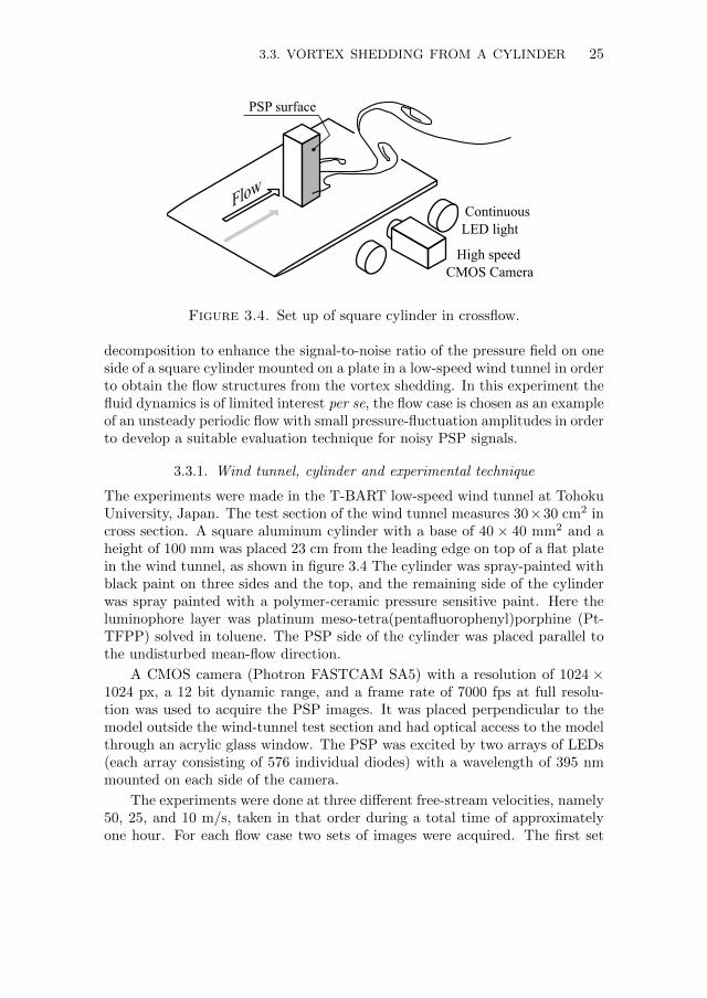
Figure 3.4. Set up of square cylinder in crossflow.

decomposition to enhance the signal-to-noise ratio of the pressure field on oneside of a square cylinder mounted on a plate in a low-speed wind tunnel in orderto obtain the flow structures from the vortex shedding. In this experiment thefluid dynamics is of limited interest per se, the flow case is chosen as an exampleof an unsteady periodic flow with small pressure-fluctuation amplitudes in orderto develop a suitable evaluation technique for noisy PSP signals.

3.3.1. Wind tunnel, cylinder and experimental technique

The experiments were made in the T-BART low-speed wind tunnel at TohokuUniversity, Japan. The test section of the wind tunnel measures 30×30 cm2 incross section. A square aluminum cylinder with a base of 40 × 40 mm2 and aheight of 100 mm was placed 23 cm from the leading edge on top of a flat platein the wind tunnel, as shown in figure 3.4 The cylinder was spray-painted withblack paint on three sides and the top, and the remaining side of the cylinderwas spray painted with a polymer-ceramic pressure sensitive paint. Here theluminophore layer was platinum meso-tetra(pentafluorophenyl)porphine (Pt-TFPP) solved in toluene. The PSP side of the cylinder was placed parallel tothe undisturbed mean-flow direction.

A CMOS camera (Photron FASTCAM SA5) with a resolution of 1024 ×1024 px, a 12 bit dynamic range, and a frame rate of 7000 fps at full resolu-tion was used to acquire the PSP images. It was placed perpendicular to themodel outside the wind-tunnel test section and had optical access to the modelthrough an acrylic glass window. The PSP was excited by two arrays of LEDs(each array consisting of 576 individual diodes) with a wavelength of 395 nmmounted on each side of the camera.

The experiments were done at three different free-stream velocities, namely50, 25, and 10 m/s, taken in that order during a total time of approximatelyone hour. For each flow case two sets of images were acquired. The first set


being wind-on conditions, i.e. with the wind tunnel and LED illuminationoperating. For each flow case a total of 19212 images were acquired at a framerate of 2000 fps. The second set of images were 1000 dark frames acquiredwithout flow and illumination, and with a frame rate and shutter speed equalto that of the wind-on images. These images were used to subtract backgrounddisturbances from the flow images.

Since the PSP degrades with time each measurement was started by ad-justing the LED strength so that the output from the camera with no flow wasabout 3000 counts out of the available sensing range of 4096. At this intensitylevel and with the used PSP the minimum detectable pressure change (onecount), or quantification error, was approximately 50 Pa. The photo degra-dation during an experiment was about 6 counts, corresponding to 300 Pa.Furthermore, the minimum detectable level also acts to filter out turbulentfluctuations, as the r.m.s. value of the turbulence is expected to be below15 Pa even at 50 m/s.

3.4. Compressor flow

The workings of a compressor is given by its performance map that showsthe pressure ratio across the compressor as function of the mass-flow rate fordifferent rotational speeds, the so called constant speed lines. The pressureratio is given as the total pressure downstream of the compressor divided bythe static pressure on the upstream side. Figure 3.5 shows a typical compressormap for a compressor of the size used here. Also shown in the map are linesof constant efficiency. As can be seen the map is limited to a certain region ofthe pressure-ratio/flow-rate plane, the left-hand side limit is denoted the surgeline, whereas the right-hand side limit is the so called choke line. The chokeline corresponds to the case of choked flow due to reaching Mach number equalto one in the “smallest” section of the compressor that makes it impossibleto increase the flow rate further. When approaching the surge line the flowseparates from the blades and it first enters into a stage called rotating stallwhereafter surge occurs and the flow rate becomes small or may even reverse.When approaching the surge line high-level noise is produced and in the fullysurge-flow region the flow conditions are so severe that it may eventual destroythe compressor.

3.4.1. Compressor test-flow facility

Although the aim of the study is to study the flow of the compressor of a tur-bocharger, the measurements were made on a compressor driven by an electricmotor, thereby obtaining both well-controlled conditions with respect to rota-tional speed as well as avoiding heat-transfer effects that may occur using aturbocharger. The motor has a maximum power of 45 kW and the rotationalspeed is frequency controlled. The maximum rotational speed of the motor is

3.4. COMPRESSOR FLOW 27

Figure 3.5. Typical compressor map.

Figure 3.6. Image of the electric motor (a) with drive belt(b) to the compressor (c). With the system for data acquisition(d).


3000 rpm. The present setup allows the compressor to be run at typical rota-tional speeds of an internal combustion engine by using both a belt drive witha drive ratio of 1:4 between the motor and the axis of a planetary gear box.The gear box has a drive ratio of 1:9.49 which allows the compressor to be runat rotational speed higher than 110 krpm, however the maximum rotationalspeed tested here was 50 krpm. The gear box and the compressor are mountedtogether in a single unit and is the commercially available Rotrex C30-74. Thecompressor wheel has seven primary and seven splitter blades and an inlet di-ameter of 51 mm. Figure 3.6 shows an image of the motor and compressor setup.

During the experiments the inlet of the compressor was open to the atmo-sphere and the inlet static pressure was hence the atmospheric pressure. Atthe outlet a plastic hose was attached and about 30 D downstream a Pitottube connected to a pressure transducer was used to measure the total pres-sure. Downstream the Pitot tube a rotary ball valve was used to control theflow rate which was measured with a turbine mass-flow meter (GL Flow FL1).An optical blade-passage sensor (Optel-Thevon 152G10) was mounted in thecompressor housing and the sensing area was directed towards the primary com-pressor blades and therefore gave seven pulses per rotation of the compressorwheel.

CHAPTER 4

Applications of PSP

The experimental work made for this thesis has largely revolved around the in-vestigation of methods suitable for the measurement of wall pressure in pulsat-ing internal flows. As such, a diversity of techniques has been used in differentexperiments in order to gain an as broad experience as possible. In this chap-ter an overview of the different instrumentation, acquisition, evaluation, andfiltering methods used is presented, often through examples from the differentexperiments.

4.1. Paint calibration

PSP is an indirect measurement technique where pressure is determined fromeither the steady state intensity or the lifetime of the luminescent radiation ofa paint coating. The relation between intensity, time constant, and pressurecan be described by the Stern-Volmer equation in the form

Iref

I=

τrefτ

= A(T ) +B(T )p

pref, (4.1)

where Iref and τref are the reference intensity and time constant correspondingto a reference pressure pref , and A and B are temperature dependent calibra-tion coefficients. In real experiments the relationship is often not completelylinear and a quadratic term is sometimes added to the right hand side of equa-tion (4.1) becoming

Iref

I=

τrefτ

= A(T ) +B(T )p

pref+ C(T )

�p

pref

�2

. (4.2)

The calibration constants can be determined using a PSP sample in a cal-ibration chamber where pressure and temperature can be controlled. It is anaccurate method in order to determine paint properties, especially for com-parison to other paint formulations since repeatability is high. The calibrationchamber used for the work in this thesis is illustrated, and depicted, in figure 4.1along with calibration data for a PtTFPP PC-PSP in figure 4.2.

29

30 4. APPLICATIONS OF PSP

Figure 4.1. Calibration chamber.

Figure 4.2. Example of calibration chamber data. Measuredpoints (•) with 95% confidence intervals and best fit to equa-tion (4.2) (—). Raw data (left) and in the form of equa-tion (4.2) (right). The encircled point indicates reference con-ditions.

4.1.1. In situ calibration

For experimental use some problems can arise when calibrating in a separatechamber. The paint sample is difficult to produce with the exact properties of

4.1. PAINT CALIBRATION 31

Figure 4.3. Calibration from in situ calibration. Pressureand intensity locations as indicated in figure inlay and linearfit (—). Flow was 40 g/s at 80 Hz pulsations.

the layer used in the experiment and the calibration constants are somewhatdependent on the illumination and acquisition methods used. For these reasonsit is often beneficial to use in situ calibration in cases where this approach ispossible.

Calibration was done in situ using two different methods in the y-junctionexperiments. These experiments where designed in such a way that the instru-mented part could be sealed from the atmosphere by closing valves upstreamand downstream of the test section, and through a small port the pressurecould be controlled externally. In this way the calibration constants could bedetermined using the same LED array for illumination, and camera for acqui-sition, as were used in the experimental measurements. Furthermore, the PSPlayer could be calibrated pixel-by-pixel, thus taking into account small spatialvariations of the calibration coefficients. Admittedly the possibility of sealingthe test section is not a reasonable option in most experimental set ups.

The other, more easily attainable, method of in situ calibration is to cali-brate the paint in post processing by using reference pressure transducers. Themethod is straightforward; pressure from the reference probes and the intensityin their proximity is used to fit the calibration constants in equation (4.1) or(4.2), and the constants are used to calculate pressure on the rest of the mea-sured surface. If the spatial temperature variation on the measured surface issmall, the method can provide accurate pressure data.

Calibration using reference pressure transducers has been very useful formeasurements in pulsating flows. As an example, calibration curves accordingto equation (4.1) for three pressure probe locations inside the y-junction isshown in figure 4.3 where a single phase-averaged period of PSP data is plottedversus data from reference transducers.


Figure 4.4. Example setup for intensity based measurements.

4.2. Instrumentation and methods for data acquisition

PSP is not only an indirect, but also an active measurement technique. Thepaint surface must be actively excited by external illumination in order toluminesce. As such, the user must select both the source of illumination andthe acquisition device to suit the conditions of the experiment. There area number of options available where pressure can be measured either over asurface area or at a single point. Furthermore, suitable instrumentation fordetermining pressure either from the steady state luminescent intensity or itslifetime, must be chosen.

4.2.1. Intensity imaging

For measurements where pressure is measured using the intensity method overa surface, continuous LED light is commonly used as an illumination source,and the luminescence is captured using digital imaging. This is also the methodused for most of the experiments included in this thesis, and a representativesetup is shown in figure 4.4.

Generally, in order to accurately extract pressure from intensity, three im-ages are required: a wind-on image, a wind-off image, and a dark frame. Thewind-on image is acquired at the actual flow conditions to be measured, withillumination light but in an otherwise dark surrounding. The wind-off image istaken at the same lighting conditions as the wind-on image but without flowand is used as the reference intensity, where reference pressure is atmospheric.Preferably it is acquired immediately after the wind-on image in order to keeptemperature differences between the two images small. Finally a dark frame is

4.2. INSTRUMENTATION AND METHODS FOR DATA ACQUISITION 33

acquired with the same exposure settings but without flow and without excita-tion light. This frame, or preferably a number of averaged frames, is subtractedfrom the wind-on and wind-off images in order to remove the inherent staticnoise of the imaging sensor, and eventual stray light in the laboratory.

4.2.2. An alternative to wind-off images for pulsating flows

For experiments in pulsating or other periodical flows where the pressure fluc-tuates about a stable mean value, it is possible to determine the pressure de-viations without the need for a separately acquired wind-off image, which isinstead substituted by the intensity at mean pressure, found from the temporalaverage of equation (4.1):

�Iref

I

�=

�A+B

p

pref

�= A+B

�p�pref

. (4.3)

Substituting pref with �p�, recalling that A+B = 1, and solving for Iref gives

Iref =�I−1

�−1. (4.4)

The method has some advantages in terms of accuracy since the reference inten-sity is acquired at the same time as the actual experiment, thus the temperatureis unchanged, and the effects of luminescent decay is kept to a minimum. Still,there will be some loss of luminescent intensity from the beginning to the endof the acquisition due to photobleaching of the luminophores.

As an example, results from the y-junction experiment (see figure 4.4)where this method has been used is shown in figure 4.5. Pressure was deter-mined using in situ calibration with reference pressure transducers and a phaseaverage is shown.

4.2.3. Scanning laser measurements

The intensity imaging method works well in most situations but can fall shortwhen very short exposure times are required, due to the low light levels reachingthe sensor. For surface measurements the user has the options of either usingan image intensifier, with the downside of an increase in stochastic noise, orincreasing the excitation light. However, considering that image intensifierscan have intensity gains in the thousands, an equivalent increase in excitationlight may be impractical for surface measurements, but, on the other hand, ifthe surface area is reduced to a single small spot, the necessary intensity levelscan readily be provided by laser light.

In the compressor measurements in paper 4 of this thesis laser light wasused as the excitation source for PSP. The basic setup is shown in figure 4.6and an image of the actual setup used is shown in figure 4.7. A laser beamwas guided through two galvanic mirrors that could guide the laser spot to anyvisible point on the PSP surface. The luminescence from the PSP was collected


Figure 4.5. Example results from y-junction experiment us-ing Iref at < p >, in situ calibration with reference pres-sure transducers, and phase averaging. The overview (top left)show the position where the time-dependent pressure is plot-ted (top right). The spatial pressure distribution (bottom) isplotted for six phase angles as indicated. The data are takenfrom an experiment with a mass flow of 130 g/s and a pulsatingfrequency of 80 Hz.

through a lens and measured using a photomultiplier tube (PMT). PMTs arelow-noise devices and can be sensitive enough to measure single photon events.They operate by the conversion of photons to electrons that amplify in cascadesinside the tube before the signal is sampled.

When measuring at one spatial point at a time, it is comparatively un-problematic to record the temporal behaviour of the luminescence instead of

4.2. INSTRUMENTATION AND METHODS FOR DATA ACQUISITION 35

Figure 4.6. Principal setup for scanning laser measurements.

Figure 4.7. Image of the setup for compressor measurementsdepicting the compressor (a) and laser scanning system withlaser head (b), galvanic mirrors (c), dichroic mirror (d), lens(e), low-pass filter (f), photomultiplier tube (g), and bladepassage sensor (h).

just its steady state intensity. This was done in the compressor experimentsand the lifetime method was used to determine the pressure.

For each spatial point to be measured on the PSP surface a 1 µs long laserpulse was shot and the paint luminescence was sampled through the PMT.The sampling was started just before the laser was shot and 30 points wereacquired at a sampling rate of 800 kHz. The first point, acquired before thelaser was shot, was subtracted from the remaining points in order to removesystem offset.


Figure 4.8. Pressure on the impeller of a radial compressorat 40,000 rpm captured using the scanning laser and lifetimemethods. Pressure over the whole visible surface (left) andalong the cord taken at center blade span (right) for each blade(gray) and the their average (black).

The points sampled after the laser pulse can be described by an exponentialdecay according to I = I0 exp(−t/τ), where τ is the luminescent lifetime andI0 is the intensity at an arbitrary starting time t0 = 0. In these experiments τwas calculated from the measured data using just I0 and the subsequent pointI1 according to τ = (t1 − t0) ln(I0/I1)−1.

The pressure was determined from the lifetimes using equation (4.2) wherethe reference lifetime, τref , was acquired on the non-rotating impeller wherepref = patm. The calibration coefficients was found from a paint sample ina calibration chamber placed directly in front of the compressor so that thesame excitation and acquisition routines could be used for the experiment andcalibration. An example of data captured using the scanning laser and lifetimemethods is shown in figure 4.8.

Since the luminescent lifetime of the paint is independent of the peak in-tensity level of the luminescence, the lifetime method has an advantage incomparison to the intensity method in that the effects of paint aging and pho-tobleaching can be almost fully eliminated.

4.3. A note on temperature errors

The calibration curves in figure 4.2 is used as an example to illustrate thetemperature sensitivity of PSP. Here the error in accuracy, as indicated by theoffset between curves of different temperatures, is about 3.5 kPa/K, and sincethe accuracy of temperature measurements are normally limited to about 0.1K;such an uncertainty is not insignificant.

4.4. NOISE REDUCTION TECHNIQUES 37

As for the error in precision, as indicated by the difference in the slopesbetween the curves of different temperatures, it is significantly smaller than theaccuracy error for most flow cases: about 3%/K in the presented sample. Thiscan be used for experiments in pulsating flow by the evaluation of pressurein terms of its temporal mean, as is described in section 4.2.2. By doing so,since no absolute pressure level is determined, only the smaller precision erroris relevant, given that the temporal temperature fluctuations remain small.

In experiments where the spatial temperature variation is small the tem-perature effects can be nearly eliminated by the use of reference pressure trans-ducers since the relationship between intensity, or lifetime, and pressure can beestablished in the actual experiment; thus the temperature of the calibrationis identically equal to the temperature of the measurement.

Rather than separately measuring spatially resolved temperatures, theabove principles has been used throughout the experiments included in thisthesis in order to minimize, rather than correct for, the effects of temperatureerrors. This has been possible since the experiments has been in pulsating flowsand/or on surfaces where spatial temperature variation has been small.

4.4. Noise reduction techniques

One problem in PSP measurements is noise, especially in low-speed flows, thatcomes from its rather low sensitivity to pressure. For the example paint withcalibration curves shown in figure 4.2, the sensitivity is about 0.5%/kPa. Forthis reason it is often necessary to filter acquired data in order to obtain usefulresults, and in this section the filtering methods used for the experiments madefor this thesis is discussed in order of increasing complexity.

4.4.1. Temporal and spatial low-pass filtering

Low-pass filtering has to be considered a standard tool for any experimentalistand the obvious use is the removal of (non-physical) high-frequency content of asignal. If we instead take the perspective of noise reduction it can be seen as anexchange of the high frequency content for better signal-to-noise ratio. Imaginean n-point moving average filter where at each point, the point itself and theprevious n − 1 points are averaged, leading to an increase in signal-to-noiseratio proportional to the square root of n, a requirement being that the noise isstochastic and uncorrelated to the signal being measured. For broadband noise,dimensionless frequencies well above 1/n are stochastic while the frequenciesbelow are not, since the points are not independent of each other. Clearly allfrequency content of the signal being measured must also be below 1/n in ordernot to be filtered out.


Low-pass filters can be configured in a number of ways in order to optimisecertain properties; e.g. maximum passband flatness, fast cutoff, or minimal sig-nal distortion; and while the relations described for the simple moving averagefilter does not hold true for all types of filters the general principle does.

Another, somewhat overlooked, advantage when using (digital) low-passfiltering is the increase of resolution under certain conditions. If for example areal signal measuring 4.3 V is sampled using an AD-converter that quantifiesthe data in 1 V steps, a single acquisition will give a 4V result, and the averageof any number of points would not decrease the measurement error. However,if white noise with a standard deviation of 1V were added to the original signalthe samples would take a range of values, still integer, but this time theiraverage would tend towards the true 4.3 V mean value as the number of samplesincrease. The technique is known as oversampling and in order to gain n extrabits of resolution 22n samples must be averaged. This potential resolution gainis available for all types of low-pass filtering but the given relation betweengain and number of samples is dependent on the method used.

In experiments using high speed imaging of PSP, signal-to-noise levels areoften rather poor and it is common to use pixel binning, i.e. reducing im-age size by replacing rectangular blocks of pixels by their mean value. Thishas the double benefit of increasing both signal-to-noise ratio and resolution.For instance, if each bin is 2 × 2 pixels, signal-to-noise ratio is improved bya factor two, and resolution by one bit. This improvement can be very valu-able, especially in unsteady low-speed flows where available light is low due toshort exposure times, and intensity variations are small due to low pressuredifferences.

4.4.2. Phase averaging

Phase averaging is a basic noise-reduction technique suitable for a periodic flowwith a stable base frequency, such as forced pulsating flow or standing acousticwaves. The main idea is to sample and average a number of points at a knownphase angle, and by repeating this for several phase angles forming an averageperiodic behaviour.

The method was used in paper 2 where pulsating pressure was measuredon an inside wall of a square y-junction. A pulsating flow was generated by arotating valve driven by an electric motor, and an angular encoder mountedto the motor axis provided the phase angle. LED light was used to excite thepaint layer and the luminescence was measured using a CCD-camera. In theseexperiments the acquisition of each specific phase angle was done by keeping thecamera shutter open while the LED’s were triggered to give a short pulse at thedetection of the phase angle currently being measured. This way the intensityof between 75 and 150, depending on the case, short pulses of luminescent lightwas added to each image. A total of 50 different phase angles were captured


Figure 4.9. Example phase avererage. Original data (- • -)with one mean period (—).

this way and together formed a period of the pulsating pressure. To furtherdecrease noise the experiment was repeated 25 times and the captured periodswere averaged.

Another option in this scenario would have been to use continuous excita-tion light and instead capture an image at each wanted phase angle, this wouldhowever have required a high frame-rate camera, or longer experiment times.

The above described method is based on images being captured at thetriggering of a known phase angle. Another method is to use high-speed imag-ing and capture a large number of frames unsynchronized with the flow, usingcontinuous light. Averaging is done such that the period of the measured flowphenomena is divided into slots of a certain length and images falling withinthese slots are averaged. For instance, if selecting phase angle steps of 5◦, thedata is phase averaged by taking the mean value of all images captured in theinterval 0◦ ≤ ϕ < 5◦, the mean value of the images captured in the interval5◦ ≤ ϕ < 10◦, and so forth. Phase information is however still needed in orderto do this sorting, and can be gathered by simultaneously sampling an angularencoder if it is a driven flow, from a pressure probe strategically placed in theflow, or in some cases from the measured data itself. When selecting a framerate for image capturing, frequencies that are multiples of the main flow fre-quency under investigation should be avoided in order to spread the imagesover the whole signal period.

For PSP measurements the unsynchronized method has some advantagesover the synchronized since the total experiment time is generally shorter, re-ducing the problems associated with temperature drift and luminescent decay.

Unsynchronized phase averaging was used for data where the y-junctionexperiment described above was repeated, but instead of using pulsating light,


the PSP was excited by a single continuous 40 W, 400 nm LED and luminescentemission was acquired using high speed imaging. For one flow case, 3000 imageswere acquired unsynchronized with the flow at a frame rate of 1500 fps, limitingthe measurement time to two seconds, practically eliminating the problems oftemperature drift and luminescent decay.

As an example, a comparison of PSP data for a flow case with a massflow of 40 g/s pulsating at 40 Hz is shown in figure 4.9 before and after phaseaveraging. Here the full period was divided into 100 slots.

4.4.3. Singular value decomposition for noise reduction

Singular value decomposition (SVD) is the factorization of a matrix A of sizem×n into its left and right singular vectors, [u1,u2, . . . ,um] and [v1,v2, . . . ,vm]respectively, as well as its singular values [σ1,σ2, . . . ,σmin{m,n}]. The singularvectors and values can be written as matrices where the left singular valuesform U of size m × m, the right singular vectors form V of size n × n, andthe singular values are in the diagonal of the matrix Σ of size m × n. Thedecomposition is done according to

A = UΣVT =

N�

i=1

uiσivT

i , (4.5)

where the left and right singular vectors are eigenvectors of AAT and A

TA

respectively. They are orthonormal, i.e. of unit length, |ui| = |vi| = 1, andperpendicular, angle(ui,uj) = angle(vi,vj) = 90◦ [i �= j], to each other. Thesingular values are the square roots of the eigenvalues of AA

T, or ATA, and

can be seen as a measure of relative energy content of the corresponding singularvectors. The singular values, and vectors, are sorted by order of descendingenergy content.

If we let A =[a1,a2, . . . ,an] represent n m-dimensional points in space anddecompose this into its singular vectors, the angle of u1 will be the direction ofmost spread (similar to the slope of a linear least square approximation throughthe origin), u2 will have the angle of most spread perpendicular to u1, u3 theangle of most spread perpendicular to u1 and u2, and so forth. The valuesof σivi give the distance from the origin to the original points perpendicularlyprojected to ui. The singular value, σi, is a scaling constant and comes from thecondition that |vi| = 1. The components of the SVD can be seen as cumulativebest fit approximations to A where u1σ1v

T1 is the best fit to A itself, u2σ2v

T2

is the best fit to A− u1σ1vT1 , and so forth.

The properties of the technique makes it well suited for separating physicalbehaviour in measurement data from stochastic noise since physical behaviour,tending to behave in a coherent manner, end up in the lower indexed, moreenergetic singular vectors while stochastic noise, acting incoherent, spread outover several higher indexed singular vectors.


Figure 4.10. First twelve left singular vectors from SVD ex-ample. Flow is from left to right.

Figure 4.11. Pressure field before (top) and after (bottom)SVD filtering. Flow is from left to right.

As an example of SVD filtering we use results from paper 3 in this thesiswhere a 40 × 40mm2 square cylinder with a height of 120 mm was placed ina cross flow of 50 m/s. PSP data was acquired from the vortex shedding onone of the sides parallel to the flow using high speed imaging under continu-ous excitation light. In the original data any vortex shedding structures areessentially drowned out by noise.

Since vortex shedding is periodic, a method of filtering that comes to mindis phase averaging (section 4.4.2). This is however not unproblematic since thefrequency of the signal is not constant over time, and also that the signal doesnot cross the mean level in each period making it difficult to define a phase.SVD on the other hand does not depend on the frequency or level of the signalbut rather on how well correlated the behaviour is; as the vortices are shed alarge number of pixels change their values in a coordinated fashion while thepixel noise behaves individually.

In order to use the filtering technique the data must first be organizedinto a two-dimensional matrix. In the example described here, 3000 consec-utive 600 × 256 pixel images were used and organized into a matrix A such


that each row represents the behaviour of one pixel in time. Now A, of size153600× 3000, was decomposed according to equation (4.5) using the MatLabcommand [U Si V] = svd(A,0);. Out of the 3000 left singular vectors in U,the first twelve, [u1, . . . ,u12], were reshaped into the original image size andare plotted in figure 4.10. Vectors u12 and above contain no visible structuredbehaviour and u2 is a result of model vibration, and from the set of 3000 vectorsonly [u1,u3 . . . ,u11] contain the vortex shedding behaviour. From these twelvevectors the data was reconstructed, again using equation (4.5), or in MatLab:m=[1 3:11]; A=U(:,m)*Si(m,m)*V(:,m)’;. The original and filtered signalsare shown in figure 4.11 and it is clear that the method has dramatically re-duced the signal noise.

CHAPTER 5

Summary of results and main conclusions

This chapter provides a summary of the contributions and conclusions of thepapers presented in Part II of this thesis.

Dynamic calibration of polymer/ceramic pressure sensitive paint

using a shock tube

• The dynamic step response of a [Ru(phen)3]2+ PC-PSP was investigatedwhere a step change in pressure was provided by a moving shock per-pendicular to a PSP surface mounted on the side wall of a shock tube.A 5 W, 465 nm LED was used for paint excitation and luminescencewas captured using a photomultiplier tube.

• The cutoff frequency of the system was estimated to a few kilohertz,which is high enough for the investigation of most behaviour encounteredin the gas-exchange processes of internal combustion engines.

• A method was proposed to compensate for dynamic errors in amplitudeand phase caused by the time delay from oxygen diffusion in the paintlayer. The method is based on the filtering of the acquired signal thr-ough an inverse of the dynamic model of the PSP using the z-transform.The method showed promising preliminary results, but due to high sen-sitivity to noise it may be impractical in real applications.

• The moving shock in a shock tube is followed by the so called contactsurface, the interface between driven and driver gas. Over the contactsurface, the pressure remains constant but the now expanded drivinggas can be of significantly lower temperature, and in these experimentsthis drop was about 500 K. This rather dramatic temperature drop wasundetected by the PSP, and it is therefore concluded that the tempera-ture seen by the PSP, when applied to metal surfaces with low thermalresistance, is that of the model surface rather than the gas temperature.This is promising for the use in pulsating flows in ICEs where temper-ature variations can be high within the cycle, but the metal surfaceshave high enough thermal mass to keep constant temperature over thecycles.

43

44 5. SUMMARY OF RESULTS AND MAIN CONCLUSIONS

Wall pressure measurements in a y-junction at pulsating flow

using polymer/ceramic pressure sensitive paint

• The pressure on the inside wall of a y-junction was measured usinga [Ru(phen)3]2+ PC-PSP. Air entering the branch of the “y” with amean massflow of 60–150 g/s for pulse frequencies up to 80 Hz. Theexit forming an acute angle to the inlet was closed while the other wasopen to the atmosphere. Paint illumination was acquired using a CCDcamera and phase averaging was done in-camera by the accumulation ofpulses from a LED array synchronized with the phase of the pulsatingflow.

• It was shown that PC-PSP could be used for spatiotemporal pressuremeasurements in internal flow in frequency ranges typical for internalcombustion engines.

• Due to short exposure times, necessary for temporal resolution in timevarying flows, phase averages had to be built up during a long time pe-riod, in order of hours for each test case. At these time scales, tempera-ture variations and photobleaching is not insignificant and the presentedresults are mostly of quantitative nature.

Enhancing signal-to-noise ratio of pressure sensitive paint data

by singular value decomposition

• A method is proposed to improve the signal-to-noise ratio of PSP datacaptured by high-speed imaging. The basis is the use of singular valuedecomposition (SVD) to extract and discard non-correlating structuresfrom the pressure field. As a test case, data (acquired by a high-speedCMOS camera) of the vortex shedding on the side of a square cylinderin cross flows between 10 and 50 m/s was used. The model was instru-mented with a PtTFPP PC-PSP that was excited by continuous lightfrom arrays of LEDs.

• Using the proposed method, stochastic pixel noise could be reduced withup to two orders of magnitude and made it possible to recover the flowstructured from the vortex shedding otherwise submerged in noise.

• Apart from stochastic noise the method also enabled the identification,and removal, of behaviour caused by model vibration. This approachmay provide a valuable tool as an alternative to image registration whenmodel movements are small.

Pressure sensitive paint measurements on a turbocharger com-

pressor

• The pressure on the impeller of a radial compressor driven by an electricmotor was measured using a scanning laser system and the lifetimemethod. The PSP used was a PtTFPP PC-PSP which was excited

5. SUMMARY OF RESULTS AND MAIN CONCLUSIONS 45

using a 405 nm diode laser. Luminescent decay was captured usinga photomultiplier tube. Complementary experiments were made usinga high-speed CMOS camera and continuous light from a single 40 W,400 nm LED.

• Using the proposed method, maps of the blade surface pressures couldbe acquired for cases measured inside the compressor map.

• For a case where the compressor operated in surge, the characteristicsurge frequency could be found, and its spatial distribution could bedetermined using the complementary measurements using high-speedimaging.

• Compared to pulsed lasers, commonly used in PIV measurements, theenergy per pulse is low for the diode laser used in these experiments.However, the very high repetition rate, 100 MHz, keeps experimenttimes short, leading to less issues with temperature variations and paintdecay. The high repetition rates also makes it possible to capture peri-odic events without the need for phase reconstruction in post processing.

• In these experiments rotational speeds could not be increased above50 krpm. This was limited by the breakdown of the optical blade passagesensor as it was covered by a fine white dust, blown off the the PSPundercoating. The limit in rotational speeds of the tested PSP itselfremains unknown.

CHAPTER 6

Papers and authors contributions

Previously published papers (1–3) included in Part II has been slightly alteredin order to fit the format of the thesis and some minor corrections have beenmade. Their content is otherwise unchanged.

Paper 1

Dynamic calibration of polymer/ceramic pressure sensitive paint using a shocktube.M. Pastuhoff (MP), N. Tillmark (NT) & P.H. Alfredsson (HAL).In Proc. 7th Int. Conf. Flow Dynamics, Sendai, Japan, pp. 132–133 (2010).

A method where the dynamic behaviour of PSP is characterized using a shocktube is presented together with a scheme for the correction of dynamic errors.The experiment was set up by MP with the help of NT. The experiment weremade and evaluated by MP and the paper was written by MP with input fromNT and HAL.

Paper 2

Wall pressure measurements in a y-junction at pulsating flow using polymer/ceramicpressure sensitive paint.M. Pastuhoff, N. Tillmark & P.H. Alfredsson.In Proc. 10th International Symposium on Experimental and ComputationalAerothermodynamics of Internal Flows, Brussels, Belgium (2011).

Pulsating pressure on the inside wall of a y-junction, sized to resemble part ofan exhaust manifold of a car engine, was measured using PC-PSP. The PSPwas excited using pulsed LED light and the luminescent intensity was capturedusing a CCD camera. Phase averaging was used to increase the signal-to-noiseratio. The experiment was set up by MP with input from NT and HAL. Dataacquisition and evaluation was made by MP and the paper was written by MPwith input from NT and HAL.

46

6. PAPERS AND AUTHORS CONTRIBUTIONS 47

Paper 3

Enhancing signal-to-noise ratio of pressure sensitive paint data by singularvalue decomposition.M. Pastuhoff, D. Yorita (DY), K. Asai (KA), & P.H. Alfredsson.Meas. Sci. Technol. 24, 075301 (2013).

A method is proposed for improving the signal-to-noise ratio of PSP data cap-tured by high-speed imaging. The basis is the use of SVD to extract anddiscard non-correlating structures from the pressure field. Previously acquiredunsteady pressure data from a square cylinder in a cross-flow was used as atest case. The experiments were suggested by KA and made by DY and MPwhen MP visited Tohoku University, Sendai, in 2012. The filtering method wasdeveloped and implemented by MP with support from HAL and the paper waswritten by MP with input from HAL.

Paper 4

Pressure sensitive paint measurements on a turbocharger compressor.M. Pastuhoff.Technical Report (2014).

The pressure on the impeller of a radial compressor driven by a electric motorwas measured using a scanning laser system and the lifetime method. Mapsof the blade surface pressures could be acquired for measurement cases insidethe compressor map. For a case in surge, the surge frequency and its spatialdistribution could be acquired.

48

Acknowledgements

This work started as a project financed through the Swedish Energy Agencyand was managed under the umbrella of the KTH Competence Center forGas Exchange (CCGEx) that also took over financial sponsoring in its laterstages. Financing was also received from “Erik Petersohns minne” and “Styffesstiftelse” for conference visits. The JSPS Global COE program sponsored asummer school at, and also a research visit to, Tohoku University. The financialsupport from all is greatly acknowledged.

——

I wish to first thank my main supervisor Henrik Alfredsson who has pushedme in the right direction when I have diverged from the path leading to thisthesis and, just as importantly, shared my enthusiasm and uninterruptedly letme do those things I do well when I have had the momentum to rush forward.My second supervisor Nils Tillmark has always been available for discussingthe next steps to take, and what choices to make at the intersections. Hisexperience and opinions has helped me immensely. I wish to also express mygratitude towards Keisuke Asai, not only for inviting me to his laboratory topartake of his vast knowledge on the topic of PSP, but also for making me feelwelcome there.

The experimental work I have done at KTH would not have been possiblewithout the toolmakers Kim and Goran who have been a constant supportin the manufacturing of the experimental equipment used. I have also hadcomrades, in Stockholm and Sendai, who have provided me with support, fun,intriguing discussions, and just the best possible working environment; I owemy gratitude to them all. I wish to especially name Sissy and Alex, whom havemade sharing an office a good thing, as well as my seniors Malte, Fredrik andBengt for teaching me the ways of the lab.

I owe the world to my family for all the support they have given me through-out the years, and to my wife Bruna, who have filled my life with warmth: Youare my home, wherever we may be.

49

References

Aider, J.-L., Elena, L., Le Sant, Y., Bouvier, F., Merienne, M.-C. & Peron,J.-L. 2001 Pressure-sensitive paint for automotive aerodynamics. In Proc. SAE

2001 World Congress. SAE transactions 2001-01-0627.

Asai, K., Nakakita, K., Kameda, M. & Teduka, K. 2001 Recent topics in fast-responding pressure-sensitive paint technology at national aerospace laboratory.In Proc. 19th Int. Congr. on Instrumentation in Aerospace Simulation Facilities,pp. 25–36. IEEE.

Asai, K. & Yorita, D. 2011 Measurements in low-speed flow – overview of recentadvancements at Tohoku University. In Proc. 49th AIAA Aerospace Sciences

Meeting . AIAA paper 2011-847.

Bell, J., Schairer, E., Hand, L. & Mehta, R. 2001 Surface pressure measure-ments using luminescent coatings. Annu. Rev. Fluid Mech. 33, 155–206.

Bencic, T. 1995 Experiences using pressure sensitive paint in NASA Lewis ResearchCenter Propulsion Test Facilities. In Proc. 31st AIAA/ASME/SAE/ASEE Joint

Propulsion Conference and Exhibit . AIAA paper 95-2831.

Bencic, T. 1997 Rotating pressure measurements on a scale model high by-pass ratiofan using PSP at NASA. In Proc. 6th Annu. Pressure Sensitive Paint Workshop,pp. 14–16.

Bencic, T. 1998 Rotating pressure and temperature measurements on scale-modelfans using luminescent paints. In Proc. 34th AIAA/ASME/SAE/ASEE Joint

Propulsion Conference and Exhibit . AIAA paper 98-3452.

Berkooz, G., Holmes, P. & Lumley, J. 1993 The proper orthogonal decompositionin the analysis of turbulent flows. Annu. Rev. Fluid Mech. 25, 539–575.

Boyle, R. 1664 Experiments and Considerations Touching Colours.http://www.gutenberg.org/ebooks/14504 (2014-08-18).

Brown, O. 2000 Low-speed pressure measurements using a luminescent coating sys-tem. PhD thesis, Stanford University.

Brown, O., Mehta, R. & Cantwell, B. 1998 Low-speed flow studies using thepressure sensitive paint technique. In Proc. 81st Fluid Dynamics Panel Sympo-

sium, pp. 31.1–13.

Bukov, A., Mosharov, V., Orlov, A., Pesetsky, V., Radchenko, V., Phonov,S., Matyash, S., Kuzmin, M. & Sadovskii, N. 1994 Optical surface pressure

50

REFERENCES 51

measurements: Accuracy and application field evaluation. In Proc. 73rd Fluid

Dynamics Panel Symposium, pp. 24.1–9.

Burns, S. & Sullivan, J. 1995 The use of pressure sensitive paints on rotatingmachinery. In Proc. Int. Congr. on Instrumentation in Aerospace Simulation

Facilities, pp. 32.1–14. IEEE.

Dowgwillo, R. M., Morris, M. J., Donovan, J. F. & Benne, M. E. 1996Pressure sensitive paint in transonic wind-tunnel testing of the F-15. J. Aircraft33, 109–116.

Engler, R., Klein, C. & Trinks, O. 2000 Pressure sensitive paint systems forpressure distribution measurements in wind tunnels and turbomachines. Meas.

Sci. Technol. 11, 1077–1085.

Engler, R., Merienne, M., Klein, C. & Le Sant, Y. 2002 Application of PSPin low speed flows. Aerospace Sci. Technol. 6, 313–322.

Fang, S., Disotell, K., Long, S., Gregory, J., Semmelmayer, F. & Guyton,R. 2011 Application of fast-responding pressure-sensitive paint to a hemispher-ical dome in unsteady transonic flow. Exp. Fluids 50, 1495–1505.

Franklin, G., Workman, M. & Powell, D. 1997 Digital Control of Dynamic

Systems. Addison-Wesley Longman.

Gardner, A., Klein, C., Sachs, W., Henne, U., Mai, H. & Richter, W. 2014Investigation of three-dimensional dynamic stall on an airfoil using fast-responsepressure-sensitive paint. Exp. Fluids 55, 55:1807.

Gordeyev, S., De Lucca, N., Jumper, E. J., Hird, K., Juliano, T. J., Gre-gory, J. W., Thordahl, J. & Wittich III, D. J. 2014 Comparison of un-steady pressure fields on turrets with different surface features using pressure-sensitive paint. Exp. Fluids 55, 1–20.

Gregory, J. 2002 Unsteady pressure measurements in a turbocharger compressorusing porous pressure-sensitive paint. Master’s thesis, Purdue University.

Gregory, J. 2004 Porous pressure-sensitive paint for measurement of unsteady pres-sures in turbomachinery. In Proc. 42nd AIAA Aerospace Sciences Meeting . AIAApaper 2004-294.

Gregory, J., Asai, K., Kameda, M., Liu, T. & Sullivan, J. 2008 A reviewof pressure-sensitive paint for high-speed and unsteady aerodynamics. Proc.

IMechE, Part G: J. Aerospace Engineering 222, 249–290.

Gregory, J., Sakaue, H., Liu, T. & Sullivan, J. 2014 Fast pressure-sensitivepaint for flow and acoustic diagnostics. Annu. Rev. Fluid Mech. 46, 303–330.

Holmes, P., Lumley, J., Berkooz, G. & Rowley, C. 2012 Turbulence, Coherent

Structures, Dynamical Systems and Symmetry , 2nd edn. Cambridge UniversityPress.

Kabral, R., Rammal, H. & Abom, M. 2013 Acoustical methods for investigatingturbocharger flow instabilities. In Proc. SAE 2013 Noise and Vibration Confer-

ence and Exhibition. SAE transactions 2013-01-1879.

Kalpakli Vester, A. 2014 Vortices in turbulent curved pipe flow. PhD thesis, KTHRoyal Institute of Technology.

Kameda, M., Tabei, T., Nakakita, K., Sakaue, H. & Asai, K. 2005 Imagemeasurements of unsteady pressure fluctuation by a pressure-sensitive coatingon porous anodized aluminium. Meas. Sci. Technol. 16, 2517–2524.

52 REFERENCES

Kavandi, J., Callis, J., Gouterman, M., Khalil, G., Wright, D., Green, E.,Burns, D. & McLachlan, B. 1990 Luminescent barometry in wind tunnels.Rev. Sci. Instr. 61, 3340–3347.

Laurantzon, F., Tillmark, N. & Alfredsson, P. H. 2010 A pulsating flow rig foranalyzing turbocharger performance. In Proc. 9th Int. Conf. on Turbochargers

and Turbocharging , pp. 363–72.

Laurantzon, F., Tillmark, N., Orlu, R. & Alfredsson, P. H. 2012 A flowfacility for the characterization of pulsatile flows. Flow Meas. Instrum. 26, 10–17.

Le Sant, Y., Bouvier, F., Merienne, M. & Peron, J. 2001 Low speed tests usingPSP at ONERA. In Proc. 39th Aerospace Sciences Meeting and Exhibit . AIAApaper 2001-0555.

Lepicovsky, J. & Bencic, T. 2002 Use of pressure-sensitive paint for diagnostics inturbomachinery flows with shocks. Exp. Fluids 33, 531–538.

Liu, T., Campbell, B., Burns, S. & Sullivan, J. 1997a Temperature and pressure-sensitive luminescent paints in aerodynamics. Appl. Mech. Rev. 50, 227–246.

Liu, T. & Sullivan, J. 2005 Pressure and Temperature Sensitive Paints. Springer.

Liu, T., Torgerson, S., Sullivan, J., Johnston, R. & Fleeter, S. 1997b Rotorblade pressure measurement in a high speed axial compressor using pressureand temperature sensitive paints. In Proc. 35th Aerospace Sciences Meeting and

Exhibit . AIAA paper 97-0162.

McLachlan, B. & Bell, J. 1995 Pressure-sensitive paint in aerodynamic testing.Exp. Therm. Fluid Sci. 10, 470–485.

Mebarki, Y. & Le Sant, Y. 2001 Pressure sensitive paint evaluation on a super-critical wing at cruise speed. J. Vis. 4, 313–322.

Middleton, W. 1963 The place of Torricelli in the history of the barometer. Isis 54,11–28.

Mitsuo, K., Asai, K., Takahashi, A. & Mizushima, H. 2006 Advanced lifetimePSP imaging system for pressure and temperature field measurements. Meas.

Sci. Technol. 17, 1282–1291.

Mitsuo, K., Egami, Y., Asai, K., Suzuki, H. & Mizushima, H. 2002 Devel-opment of lifetime imaging system for pressure-sensitive paint. In Proc. 22nd

Aerodynamic Measurement Technology and Ground Testing Conference. AIAApaper 2002-2909.

Mitsuo, K., Nakakita, K. & Kurita, M. 2004 Application of pressure-sensitivepaint to low-speed wind tunnel testing at Japan Aerospace eXploration Agency.In Proc. 24th Int. Congr. of Aeronautical Sciences, vol. 3, pp. 1–10.

Morris, M. 1995 Use of pressure-sensitive paints in low-speed flows. In Proc. 19th

Int. Congr. on Instrumentation in Aerospace Simulation Facilities, pp. 31.1–10.IEEE.

Moshasrov, V., Radchenko, V. & Fonov, S. 1998 Luminescent Pressure Sensors

in Aerodynamic Experiments. Central Aerohydrodynamic Institute (TsAGI).

Nakakita, K. 2007 Unsteady pressure distribution measurements around 2d-cylinders using pressure-sensitive paints. In Proc. 25th AIAA Applied Aerody-

namics Conference. AIAA paper 2007-3819.

REFERENCES 53

Nakakita, K. & Asai, K. 2002 Pressure-sensitive paint application to a wing-bodymodel in a hypersonic shock tunnel. In Proc. 22nd AIAA Aerodynamic Measure-

ment Technology and Ground Testing Conference. AIAA paper 2002–2911.

Nakakita, K., Yamazaki, T., Asai, K., Teduka, N., Fuji, A. & Kameda, M.2000 Pressure sensitive paint measurement in a hypersonic shock tunnel. InProc. 21st AIAA Aerodynamic Measurement Technology and Ground Testing

Conference. AIAA paper 2000-2523.

Navarra, K. 1997 Development of the pressure sensitive paint technique for advancedturbomachinery applications. Master’s thesis, Virginia Polytechnic Institute.

Navarra, K., Rabe, D., Fonov, S., Goss, L. & Hah, C. 2001 The application ofpressure-and temperature-sensitive paints to an advanced compressor. J. Turbo-mach. 123, 823–829.

Nobach, H., Tropea, C., Cordier, L., Bonnet, J., Delville, J., Lewalle, J.,Farge, M., Schneider, K. & Adrian, R. 2007 Springer Handbook of Exper-

imental Fluid Mechanics, chap. 22.4 Proper Orthogonal Decomposition: POD,pp. 1346–1369. Springer, editor: Tropea, C. et al.

Pastuhoff, M., Kalpakli, A. & Alfredsson, P. H. 2013a Pressure and velocityfield measurements of pulsating flow in a square channel y-junction. In Proc.

66th Ann. Meeting of the APS Division of Fluid Dynamics.

Pastuhoff, M., Tillmark, N. & Alfredsson, P. H. 2010 Dynamic calibration ofpolymer/ceramic pressure sensitive paint using a shock tube. In Proc. 7th Int.

Conf. on Flow Dynamics, pp. 132–133.

Pastuhoff, M., Yorita, D., Asai, K. & Alfredsson, P. H. 2013b Enhancing thesignal-to-noise ratio of pressure sensitive paint data by singular value decompo-sition. Meas. Sci. Technol. 24, 075301.

Sakamura, Y., Suzuki, T. & Matsumoto, M. 2003 Surface pressure distributionimaging at frame rates over 1 khz using porous pressure-sensitive paint. In Proc.

20th Int. Congr. on Instrumentation in Aerospace Simulation Facilities, pp. 363–371. IEEE.

Sakaue, H., Matsumura, S., Schneider, S. & Sullivan, J. 2002 Anodized alu-minum pressure sensitive paint for short duration testing. In Proc. 22nd AIAA

Aerodynamic Measurement Technology and Ground Testing Conference. AIAApaper 2002-2908.

Sakaue, H. & Sullivan, J. 2001 Time response of anodized aluminum pressure-sensitive paint. AIAA J. 39, 1944–1949.

Schairer, E., Hand, L., Bell, J. & Mehta, R. 1998 Application of pressure-sensitive paint to helicopter rotors. In Proc. 6th Annu. Pressure Sensitive Paint

Workshop.

Shimbo, Y., Asai, K. & Komatsu, N. 2000 Pressure sensitive paint application atlarge production wind tunnels. In Proc. 22nd Congr. of the Int. Council of the

Aeronautical Sciences. Paper ICAS 2000-3.3.3.

Strang, G. 2007 Introduction to Linear Algebra, 2nd edn. Wellesley-CambridgePress.

Tiikoja, H., Rammal, H., Abom, M. & Boden, H. 2011 Investigations of automo-tive turbocharger acoustics. In Proc. 10th Int. Conf. on Engines and Vehicles.SAE transactions 2011-24-0221.

Tillmark, N. & Alfredsson, P. H. 2004 Calibration and use of pressure sensitivepaint (PSP) for a transonic flow application. In Proc. 17th Symp. on Measuring

Techniques in Transonic and Supersonic Flow in Cascades and Turbomachines.

Torgerson, S., Liu, T. & Sullivan, J. 1996 Use of pressure sensitive paints in lowspeed flows. In Proc. 19th Advanced Measurement and Ground Testing Technol-

ogy Conference. AIAA paper 96-2184.

Torgerson, S., Liu, T. & Sullivan, J. 1998 Rotor blade pressure measure-ment in rotating machinery using pressure and temperature paints. In AGARD

Conf. Proc. Advanced Non-Intrusive Instrumentation for Propulsion Engines,pp. 19.1–9.

Troyanovsky, I., Sadovskii, N., Kuzmin, M., Mosharov, V., Orlov, A.,Radchenko, V. & Phonov, S. 1993 Set of luminescence pressure sensors foraerospace research. Sensor. Actuat. B-Chem. 11, 201–206.

Tsuji, Y., Fransson, J., Alfredsson, P. & Johansson, A. 2007 Pressure sta-tistics and their scaling in high-Reynolds-number turbulent boundary layers. J.Fluid Mech. 585, 1–40.

Yorita, D., Numata, D., Nagai, H. & Asai, K. 2010 Measuring unsteady low-speed flow phenomena by using a time-series analysis of pressure-sensitive paintimages. In Proc. 14th Int. Symp. on Flow Visualization. ISFV14-9E-1.

Part II

Papers

(Papers not included in online version.)

Documents

Measuring with pressure sensitive paint in time-varying …kth.diva-portal.org/smash/get/diva2:740366/SUMMARY01.pdf · Measuring with pressure sensitive paint in time ... Increasingly