MEASURING MECHANICAL BEHAVIOR OF STEEL DURING

SOLIDIFICATION: MODELING THE SSCC TEST

Matthew Rowan1, Brian G. Thomas1, Christian Bernhard2, Robert Pierer2

1 - University of Illinois at Urbana-Champaign, Department of Mechanical Science and Engineering,

1206 W. Green St., Urbana, IL, USA 61801

2 - Christian Doppler Laboratory for Metallurgical Fundamentals of Continuous Casting

Processes (MCC), Department of Metallurgy, University of Leoben, Austria

A-8700 Leoben, Franz-Josef-Straße 18

Abstract

The Submerged Split Chill Contraction (SSCC) test can measure forces in a solidifying

steel shell under controlled conditions that match those of commercial casting processes. A

computational model of this test is developed and applied to increase understanding of the

thermal-mechanical behavior during initial solidification of steel. Determining the stress profile

is difficult due to the complicated geometry of the experimental apparatus and the non-uniform

temperature and strength across the shell. The two-dimensional axisymmetric elastic-viscoplastic

finite-element model of the SSCC test features different mechanical properties and constitutive

equations for delta-ferrite and austenite that are functions of both temperature and strain rate.

The model successfully matches measurements of 1) temperature history; 2) shell thickness; 3)

solidification force; and 4) failure location. In addition, the model reveals the stress and strain

profiles through the shell and explains what the experiment is actually measuring. In addition to

the strength of the shell, the measured force is governed by the strength of junction between the

upper and lower test pieces and depends on friction at the shell / cylinder interface. The SSCC

test and validated model together is a powerful analysis tool for mechanical behavior, hot tear

crack formation and other phenomena in solidification processes such as continuous casting.

Introduction

Fundamentally-based computational models are useful tools for understanding and solving

problems in commercial casting processes . To find the material properties needed for the

models, requires controlled laboratory experiments. This work combines these two tools to gain

new insight into both the mechanical behavior of a solidifying steel shell, and the experiments

used to measure that behavior.

The Submerged Split Chill Contraction (SSCC) test is a controlled laboratory experiment

to measure the force generated in a steel shell as it solidifies and contracts around a solid

cylinder that is suddenly immersed into molten steel [1]. This test, pictured in Figure 1, is a

simplified form of the Submerged Split Chill Tensile (SSCT) experiment developed by

Ackerman et al, and since applied by [2-4]. The SSCC test body consists of two separate solid-

steel pieces shown in Figure 2. Most of the outer surface of both bodies is sprayed with a 0.4 ±

0.02 mm ZrO2 layer to control the heat flux to match the heat transfer conditions found in

continuous casting. A steel shell solidifies with the primary dendrite growth direction

perpendicular to the interface. The relative vertical position of the tops of the two pieces is held

constant by a servo-hydraulic cylinder. During solidification, a load cell measures the vertical

force that is needed to maintain the vertical positions of the pieces. This generates membrane

stresses in the shell across the dendrites with the same orientation experienced in commercial

casting processes. After ~25 sec, the test body is removed from the melt. This causes the axial

force to decrease to zero, so further contraction causes shrinkage stresses to increase mainly in

the radial and circumferential directions. After cooling to room temperature, the shell is

detached, cut, and analyzed metallographically for hot-tear cracks. This test is highly repeatable

[8] and has been used to investigate force-time [5] and stress-strain [2-6] relationships, shell

strength [7], microstructure morphology [6, 9, 10] , and various defects for many different steel

compositions [1], other castable metal alloys [11], and cooling rates [12].

Unfortunately the SSCC experiment yields little information about its fundamental

operation, including what force is being measured,and its relationship to the high-temperature

thermal-mechanical behavior of the solidifying steel that is sought. The measured force is a

single time-varying scalar taken at a single location far away from the steel shell that forms at the

interface of a complex 3D structure. How the local temperature, strain, and stress profiles evolve

within the shell and lead to hot-tear cracks cannot be determined using only this test.

In this paper, a transient finite-element model of the SSCC test is developed and applied

to gain better understanding of the thermal-mechanical behavior of steel during initial

solidification. Separate constitutive models of the thermal-mechanical behavior for austenite

[13] and delta-ferrite [12] were developed in previous by empirically fitting measured data [15,

16] to determine the relation between stress, strain, strain rate, temperature and carbon content.

These models for the separate phases were incorporated into an efficient numerical methodology

of modeling solidification developed by Koric [17] and implemented into the commercial

software ABAQUS [18]. This modeling approach has been used for a wide range of applications

including stress development in solidifying steel [17] and the formation of longitudinal face

cracks [19]. However, the constitutive equations were developed based on tensile test and creep

experiments on solid steel that was reheated after solidification and cooling. The differences

relative to the mechanical properties during solidification are unknown.

By calibrating the computational model to match the temperature and force

measurements of the SSCC test, additional insights can be gained into initial solidification that

are more powerful than either of these two tools used separately.

Previous Experiments

Attempts to understand the behavior of solidifying steel have been ongoing for centuries.

Only recently have methodologies been developed to quantify its thermal-mechanical properties

and to predict the formation of defects, using both measurements and computational models.

Initial efforts applied standard mechanical tests to reheated solid samples, including high-

temperature tensile tests [15, 16] and creep tests [20, 21]. Wray conducted tensile tests on steel

heated in a vacuum furnace from room temperature for both austenite at 950 – 1350 oC [15] and

delta-ferrite at 1200-1525 oC [16] at strain rates ranging from 10-5 - 10-2 sec-1. Strength

decreased exponentially with increasing temperature towards the solidus and at lower strain rates

[15,16] in accordance with observations of other metals [22-27]. Austenite was shown to have

much higher strength than delta-ferrite at the same temperature and strain rate [15, 16].

Creep tests on reheated steel samples have been performed primarily to investigate

bulging during continuous casting [20, 29]. In creep tests by Suzuki, 5 mm diameter cylindrical

test specimens were machined from as cast-steel and subjected to constant stress levels of 4.1 -

9.8 MPa and temperatures of 1250 - 1400 oC for ~1000 s [30, 21]. The direction of loading with

respect to dendrite growth direction did not have an effect on the creep curves [30]. Austenite

recrystallization was observed at 1350 oC at 7.1 MPa where strains above 0.1 were produced

[30].

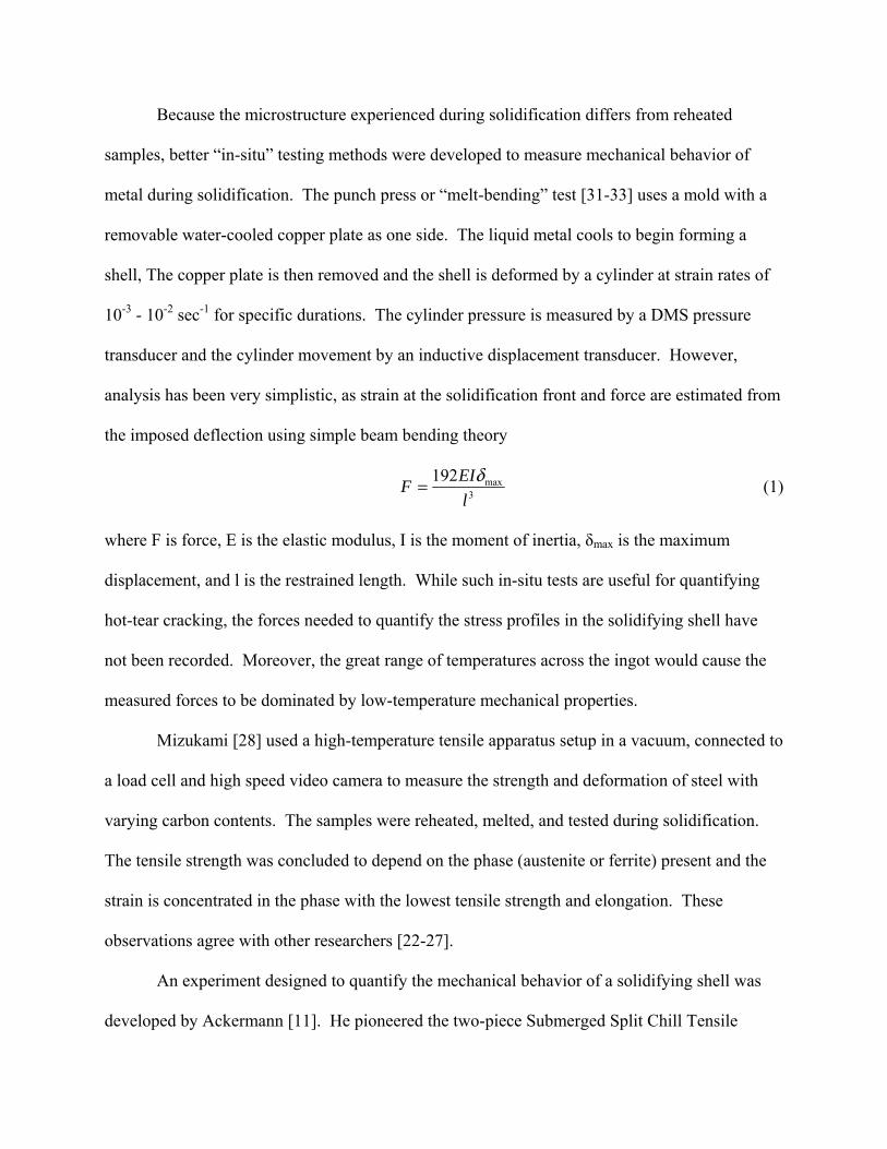
Because the microstructure experienced during solidification differs from reheated

samples, better “in-situ” testing methods were developed to measure mechanical behavior of

metal during solidification. The punch press or “melt-bending” test [31-33] uses a mold with a

removable water-cooled copper plate as one side. The liquid metal cools to begin forming a

shell, The copper plate is then removed and the shell is deformed by a cylinder at strain rates of

10-3 - 10-2 sec-1 for specific durations. The cylinder pressure is measured by a DMS pressure

transducer and the cylinder movement by an inductive displacement transducer. However,

analysis has been very simplistic, as strain at the solidification front and force are estimated from

the imposed deflection using simple beam bending theory

3max192

l

EIF

δ= (1)

where F is force, E is the elastic modulus, I is the moment of inertia, δmax is the maximum

displacement, and l is the restrained length. While such in-situ tests are useful for quantifying

hot-tear cracking, the forces needed to quantify the stress profiles in the solidifying shell have

not been recorded. Moreover, the great range of temperatures across the ingot would cause the

measured forces to be dominated by low-temperature mechanical properties.

Mizukami [28] used a high-temperature tensile apparatus setup in a vacuum, connected to

a load cell and high speed video camera to measure the strength and deformation of steel with

varying carbon contents. The samples were reheated, melted, and tested during solidification.

The tensile strength was concluded to depend on the phase (austenite or ferrite) present and the

strain is concentrated in the phase with the lowest tensile strength and elongation. These

observations agree with other researchers [22-27].

An experiment designed to quantify the mechanical behavior of a solidifying shell was

developed by Ackermann [11]. He pioneered the two-piece Submerged Split Chill Tensile

(SSCT) test, by plunging water-cooled copper cylinders directly into an aluminum melt. After

allowing time for the growing shell to reach a desired thickness, the two pieces of the cylinder

were separated, which applied a tensile load perpendicular to the direction of primary dendrite

arm growth. This allowed measurement of the strength near to the mushy zone. Ackermann

found considerable strength for solid fractions greater than 0.95 and virtually no strength below

this solid fraction.

The most sophisticated experimental apparatus to determine the strength of a solidifying

shell was accomplished by Bernhard and coauthors [34-36]. Their SSCT test is a refined version

of Ackermann’s experiment with better repeatability. It has also been used to determine the

susceptibility of forming hot tear cracks for steels with a wide range of carbon and other alloying

content [1, 37, 38]. Bernhard compared SSCT test results to other measurements of thermo-

mechanical behavior of reheated solid samples. The tensile strength near the solidus temperature

was found to be about 50% less than other measurements for austenite [39,40] due to the SSCT

test being more sensitive to effects of segregation. Tests involving delta-ferrite matched

measurements made by Wray [16], which was attributed to the negligible sensitivity of delta-

ferrite to microstructural effects.

All of these tests reveal only a single measurement about the complex multidimensional,

multi-scale mechanical behavior during solidification of a steel shell. Only by developing a

realistic mathematical model of this behavior, including its spatial and time variations can the

experimental measurement be translated into real understanding.

Hot Tearing

Cracks can occur in steel due to tensile stress combined with any of several different

embrittelement mechanisms, which span a wide range of temperatures. Hot tearing is distinct in

that it develops near the solidus temperature [41], due to strain concentration in the liquid phase

between dendrites which cannot be accommodated by liquid feeding. Hot tearing affects all

alloys, but increases with increasing difference between the liquidus and solidus temperatures

[42]. It is aggravated by the partitioning of alloying elements via segregation during

solidification. Segregation, in turn, is worsened by the slow diffusion in the solid phase, relative

to the liquid, and results in small-scale compositional variations. The result is local suppression

of the solidus temperature, which increases the size of the mushy zone and makes the steel more

susceptible to forming hot tears.

Owing to the great complexity of the phenomena that result in hot tearing, a fundamental

theory to predict this defect is too difficult. Thus, research has instead focused on developing

simple empirical models to predict hot tear formation, based on fitting experimental

measurements. Rappaz [43] proposed a hot tearing criterion with the physical basis of when the

applied tensile stress causes pressure in the liquid in the mushy zone drops low enough to

nucleate voids due to cavitation. Other simpler criteria, such as those postulated by Clyne-

Davies [44], Feurer [45] and Katgerman [46] include the effects of phase fractions, casting

conditions and calculation of the temperature zone most likely to form hot tears. Other criteria

are derived from empirically fitting experimental data to determine strain [47, 48-50], strain rate

[43, 51-57] and stress [7, 47, 58-60] levels that coincide with hot tear formation.

Pierer [7] compared stress based [61], strain based [62], strain rate based [63] and the

Clyne-Davies model [64] with experimental data from SSCT tests. He found that even though

each criterion approaches the problem from a different perspective, the predictions of cracking

susceptibility are nearly the same.

Previous Thermal-Mechanical Models

Initial endeavors to apply computational modeling to the high temperature thermal-

mechanical behavior of steel solidification began with a semi-analytical solution of the elastic-

plastic behavior of a semi-infinite steel plate prevented from bending [65] and models of the

thermal stresses that develop in the shell in and below the mold [66, 67]. Computational

modeling evolved to more complex behavior including coupling the heat conduction and

mechanical equilibrium equations with creep [68, 69] and elastic-viscoplastic behavior [14, 17,

70-73]. Koric, Thomas and coauthors implemented the Kozlowski III model for austenite [13]

and the Zhu model for delta-ferrite [14] into both implicit [17] and explicit [77] integration

schemes to model the high temperature behavior of steel. These models have been applied to

predict crack formation during continuous casting [19].

Several computational models of the SSCT [6] and SSCC [1] tests have been performed

to study phenomena such as shell strength [74, 75], grain size [9], hot tearing [1, 38, 10, 76], and

to evaluate proposed constitutive models [94]. Due the complexity of the phenomena, many

aspects of the test are still not fully understood.

Experimental Methodology

In this work, Submerged Split Chill Contraction (SSCC) experiments on steel

solidification were performed at the Christian Doppler Laboratory, University of Leoben, Austria

[1]. A photograph and schematic of the SSCC test body is given in Figure 1. The test body is

composed of two main pieces. The “lower part”, consists of two stacked cylinders on a common

centerline. The larger lower cylinder has a radius of 26 mm and length of 48 mm and is spray

coated with a 0.4 mm thick ZrO2 layer to control the heat flux to levels experienced in

commercial continuous casting processes. The smaller upper cylinder of the lower part has a

radius of 10 mm and length of 98 mm. The second major piece is a geometrically-complex

“upper part”. The dimensions of both parts are given in Appendix A, Figure A-1.

The top surface of upper part is welded to a fixed steel plate with a hole through which

the smaller upper cylindrical portion of the lower part can move. A servo-hydraulic loader

controls the alignment of these two parts. A gap of 4 mm separates the large radius of the lower

part from the inner wall of the upper part sleeve.

The assembly of the upper and lower parts, initially at room temperature, is immersed

into molten steel, causing a shell to solidify normal to the external surface and at the melt – air

interface as shown in Figures 2 (a-c). During the experiment, the temperature at the SSCC

cylinder-steel melt interface decreases causing a shell to form and subsequently desire to shrink

due to thermal contraction. However, being in contact with the heating and expanding test body,

shrinkage of the solidifying shell is prevented. The net force exerted by the solidifying shell lifts

up on the lower part and pulls down on the upper part, but the servo-hydraulic loader prevents

any vertical motion. The force required to maintain the relative positions of the upper and lower

parts is applied by the servo – hydraulic loader and is the measured ‘solidification force’.

Four thermocouples record temperature histories at different locations: two are located

inside the test body 2 mm from the steel melt interface while the other two are located in the

steel melt 20~25 mm away from this interface. Each pair of thermocouples is positioned on

opposite sides of the test cylinder, 180o apart. The pour temperature was measured prior to

immersing the SSCC test body into the steel melt and was superheated 20 oC above the liquidus

temperature.

The test body is immersed for a period of ~ 20-30 seconds. Then the test body along

with the attached steel shell is removed from the melt and cooled to room temperature. This

process is shown in Figure 2 (a-c). The shell is then detached from the test body and cut into 16

separate pieces, 8 from each half, as shown in Figure 3. The shell thickness is measured at

multiple locations per sample and then micro-analyzed to determine if any defects are present.

The steel melt alloy analyzed in this study is given in Table 1.

Table 1: Composition of Experimental Steel Alloy

%C %Mn %S %P %Si %Al %Fe

0.315 1.44 0.0051 0.0039 0.356 0.0715 Balance

Computational Model

A transient two-dimensional finite-element model of the entire SSCC test has been

developed at the Metals Processing Simulation Laboratory at the University of Illinois at

Urbana-Champaign, taking advantage of the cylindrical symmetry of the process. It consists of

separate heat transfer and mechanical models of both test body pieces, the solidifying steel shell,

and the surrounding liquid.

Heat Conduction Model Governing Equations

Heat transfer in the test body and shell is governed by the energy conservation equation.

The transient heat conduction model is two-dimensional axisymmetric ,with a Lagrangian

reference frame (no material velocities) or and no heat generation and is governed by eq. (2).

' 1p

T T Tc rk k

t r r r z zρ ∂ ∂ ∂ ∂ ∂ = + ∂ ∂ ∂ ∂ ∂

(2)

where ρ is the temperature dependent density, 'pc is the temperature and solid fraction dependent

specific heat, T is temperature, t is time, k is the temperature dependent thermal conductivity, r is

the radial coordinate and z is the vertical coordinate. The latent heat effects during solidification

are included as an adjustment to the specific heat term as a function of solid fraction when

cooling between the liquidus and solidus temperatures according to eq. (3).

' sp p f

dfc = c L

dT− (3)

where cp is found from eq. 3B in the appendix, Lf is the latent heat, assumed to be 271,000 J/kg

and fs is the solid fraction.

Mechanical Model Governing Equations

Strains that develop during solidification are small, so the small strain assumption is used

for formulating the mechanical behavior. The linearized strain tensor is

( )[ ]Tuu ∇+∇=

2

1ε (4)

The spatial displacement gradient ruu ∂∂=∇ /

is small and the Cauchy stress tensor is balanced

by the body forces, b, according to the initial configuration of the material as:

[ ] b+⋅∇ σ =0 (5)

Details of the derivation of these material states are given elsewhere [19].

The total strain rate is represented by summation inclusion of the elastic, inelastic (plastic

+ creep) and thermal components:

thermalinelaticelastic εεεε ++= (6)

The stress rate depends on the elastic strain rate only for this particular case where large rotations

are negligible and the material having a linear isotropic behavior

( )thermalinelasticD εεεσ −−= : (7)

where D is the fourth order isotropic tensor of elasticity

IIkID B ⊗

−+= μμ

3

22 (8)

with μ and kB being the temperature dependent shear and bulk modulus respectively, I and I are

the fourth and second order identity tensors.

Determination of the Thermal Strain

Volume changes caused by temperature differences and phase transformations must be

considered. The thermal strain tensor is found from eq. (9).

( ) ( )=T

T

ijijthermal dTT0

δαε (9)

where α(T) is the temperature dependent coefficient of thermal expansion, T0 is the reference

temperature and δij is the Kronecker delta.

The thermal expansion coefficient is found by computing the slope of the thermal linear

expansion (TLE) vs. temperature curve. The reference temperature was chosen to be 300 oC

with a reference TLE of -1.66 x 10-2(-).

( )ref

ref

TLE TLE Tα

T T

−=

− (10)

Determination of the Inelastic Strain

The elastic-viscoplastic response of the solidifying steel shell is modeled by using

separate constitutive equations to calculate the inelastic strain rate in the liquid, delta-ferrite and

austenite phases.

The delta ferrite model [14] is a power law empirical fit that relates the stress, σ, inelastic

strain, εinelastic, temperature, T, carbon content, %C and several empirical parameters to the

inelastic strain rate, given in eq. (11)

( )( )

( ) ( )

( ) ( )( )

( )( )

-2

n

m

inelastic-1inelastic -5.52

-5.56×104

-5

-1-4

σ MPa 1 + 1000 εε sec = 0.1

T Kf %C

300

f %C =1.3678 × 10 %C

m = -9.4156×10 T K + 0.3495

n = 1.617×10 T K - 0.06166

⋅

(11)

The austenite model [13], given in eq. (12) was developed as a curve fit to measurements

made by Wray [15, 16] and creep tests by Suzuki [21].

( ) ( ) ( ) ( )( ) ( )( )

( )( ) ( )( )( ) ( )

( )( ) ( )( ) ( )

4f -1-1 2

inelastic 1 inelastic inelastic

-31

-32

-33

4 4

-4.465×10 Kε sec =f %C σ MPa - f T K ε ε exp

T K

f T K = 130.5 - 5.128 10 T K

f T K = -0.6289 + 1.114 10 T K

f T K = 8.132 - 1.54 10 T K

f %C = 4.655 10 + 7.14 10 %C + 1.

⋅

⋅

⋅

⋅ ⋅

( )252 10 %C⋅

(12)

Where temperature is above the solidus, the liquid model is used. The liquid is modeled

as an elastic – perfectly plastic material with an elastic modulus of 10 GPa, a low yield stress of

0.01 MPa and Poisson’s ratio of 0.3. The validity of using this method is found elsewhere [77].

The effectiveness of using separate constitutive model for austenite and delta – ferrite to

predict the tensile behavior of the Wray [15, 16] and Suzuki [21] experiments has been shown

elsewhere as well [78]. Figure 4 [78] shows that the constitutive models for delta-ferrite and

austenite match well with tensile data from Wray for samples strained to 5%. This figure also

shows that delta-ferrite and mixtures of delta-ferrite and austenite are both considerably weaker

than austenite alone. There is no clear transition for the stress magnitude during the phase

transformation other than a steep increase in the stress at low delta-ferrite phase fractions. This

is incorporated into the model by assuming that if the temperature is below the solidus and the

delta – ferrite phase fraction exceeds 10%, then the delta – ferrite constitutive model is used, eq.

(11). Otherwise, for temperatures below the solidus, the constitutive equation for austenite is

used, eq. (12). If the temperature is greater than the solidus, then the elastic – perfectly plastic

model of liquid is used.

Other Thermal and Mechanical Properties

The temperature dependent thermal conductivity, specific heat and thermal linear

expansion (TLE) for the steel listed in Table 1 were obtained from the software package CON1D

v.9.7 [79]. The density was adopted from Harste [80, 81] and Jimbo and Cramb [82] and

depends on phase fractions. The thermal expansion coefficient was determined from the slope of

the TLE curve. The elastic modulus was determined from data from Mizukami [83].

The phase fractions were determined from CON1D using the segregation analysis

procedure outlined by Won [84]. The liquidus temperature was found to be 1500.95 oC, the

solidus temperature 1430.1 oC and the peritectic reaction occurs at 1486.4 oC. The phase fraction

history, thermal conductivity, specific heat, density, thermal expansion coefficient and elastic

modulus for the steel in Table 1 along with the determining equations for determining each

property are given in Appendix B.

Finite Element Implementation

The governing differential equations defined at the integration points in each element by

the results of the constitutive, eqs. (11 and 12), is transformed into two integrated equations by

invoking the backward Euler method and is solved by using a specialized Newton-Raphson

method [10, 13, 85]. The updated global equilibrium equations are then solved using the non-

linear procedures in the commercial software ABAQUS v. 6.9-1[18].. This approach has been

successfully implemented [17, 59] and has been validated by matching temperature and stress in

the semi-analytical solidification problem posed by Boley and Weiner [65]. The modeled

domain, shown in Figure 5, uses a total of 35,100 4-node linear axisymmetric finite elements for

the upper part, lower part, ZrO2 layer and steel melt. The mesh resolution was variable with

those regions of the melt that solidify having 0.25 x 0.25 mm elements which transition

gradually in regions that remain all liquid to 5.2 x 5.2 mm elements at the container wall. These

variable element sizes were chosen to reasonably determine the stress and temperature gradients

in the shell during solidification without incurring a large computation cost. Each simulation

required ~11 hours CPU time on a 3.1 GHz, 64-bit personal computer.

Boundary Conditions

The radial displacement of the upper and lower parts is restricted at the centerline due to

symmetry. Restriction of the vertical direction displacement are enforced at the top edge of the

lower and upper parts to impose the physical restraints of the hydraulic cylinder and welded steel

plate. Zero traction boundary conditions were applied to the steel melt at the top, right and

bottom edges. Zero heat flux boundary conditions are applied at the line of symmetry, as well as

at the bottom and right edge of the melt.

Immersion of the test body is modeled by varying the heat transfer coefficient (HTC)

between the steel melt and SSCC body with time and position. The origin of the model is

located in the lower left corner. The interface of the test body and steel melt is treated with a

Langrangian reference frame fixed on the test body, in which the melt moves in the positive z-

direction upward along the test body. At time t = 0 sec, the bottom edge of the test body is 0.04

m from the origin. The three distinct regions in Figure 5 of the two test body-melt interfaces

indicate the use of different coefficients of friction and heat transfer coefficient values.

Assuming that the immersion velocity, Vz, is 0.1 m/sec, the interfacial boundary conditions are:

z

z

z2

z

z

0, 0.040 m V t 0

1850, 0.047 m V t 0.040 mW

HTC 2500, 0.088 m V t 0.047 mm K

1850, 0.110 m V t 0.088 m

0, V t 0.110

> ⋅ > ≥ ⋅ ≥ = > ⋅ >

≥ ⋅ ≥ ⋅ >

(13)

These boundary conditions indicate that the bottom surface of the lower part touches the

melt at 0.4 sec into the simulation and was chosen to verify the immersion effect on the melt and

cylinder thermocouple measurements. The melt thermocouple touches the top surface of the

melt at 0.7 s, and complete immersion occurs at 1.1 s. The HTC values were selected to best

match thermocouple measurements and solidified shell thickness contours and are implemented

into ABAQUS using a GAPCON subroutine. Convection and radiation from the top surface of

the steel melt is simulated by assuming a heat transfer coefficient of 10 W/m2/K and emissivity

of 0.28 to ambient air at 30 oC.

The frictional interaction between the SSCC body and melt is separated into two distinct

regions. The coefficient of friction between the steel melt and ZrO2 was assumed to be 0.4

(labeled ‘B’ in Figure 5). The coefficient of friction between the steel melt and all other

interfacial regions was assumed to be 0.3 (labeled ‘A’ in Figure 5).

Results

Owing to the hostile, high-temperature environment of the solidifying steel experiment,

only a few measurements are possible. Without an accurate model, this data is very difficult to

interpret. The first step in a complete interpretation of the data is to ensure that the model

simultaneously matches all of experimental measurements, including thermocouple temperature

histories, final solidified shell thickness profile, reaction force history, and the location of cracks.

Temperature

Temperature has a great influence on stress during solidification, so it is not possible to

predict stresses without first achieving accurate temperature histories. Matching the measured

cylinder temperatures is important to verify that reasonable thermal properties and boundary

conditions are being used. A comparison of the thermocouple measurements and the

corresponding simulated nodal temperature histories in the SSCC cylinder body is given in

Figure 6 (a). The difference between the simulation and the cylinder thermocouple TC-2 is less

than the difference between the two measurements. Differences between the measurements may

be due to asymmetry in the placement of the thermocouples. Note that there is a short delay in

the onset of increasing temperature in the cylinder. This is due to immersion of the SSCC body.

The initial temperature of the measurements is near 40 oC even though the room temperature was

closer to 30 oC. This can be attributed to the SSCC body being suspended over the melt for a

time period before the experiment began and being heated slightly from convection and radiation

from the steel melt. The simulation of the melt temperature, shown in Figure 6 (b), closely

matches both measurements at early times. The sudden increase in the melt thermocouple, TM-

1, around 10 sec and decrease of TM-2 around 16 sec is due to thermocouple failure.

Figure 7 labels different regions of the interface between the melt and the test cylinder

around the interior perimeter of the shell. Starting at the melt surface, the interface includes the

melt contacting the upper part, air gap, lower part, ZrO2 layer and the bottom of the lower part.

Figure 8 plots temperature along this interface at different times.

Figure 8 reveals that the shell temperature at 7 sec is still slightly above the solidus

temperature at region ‘6’. At 7.1 sec, the entire interface has cooled below the solidus

temperature. For later times of 15 and 25 sec significant additional cooling of the shell is only

found in regions 1, near the top surface of the melt and at regions 8 and 9, where the ZrO2 layer

exists.

Figure 9 shows relevant temperature contours, which includes a mirrored image to give a

2-D cross sectional representation, along with a close-up of the melt at the interface with the

upper part at the end of the simulation and a scale representation of the shell. The contours

represent the liquidus, 10% solid fraction, peritectic, 90% solid fraction, 99% solid fraction and

solidus temperatures. Following the shape of the 10% solid fraction contour, it is apparent that

the shape is similar to the photo of the test after it has been removed from the melt, including the

formation of solid shell at the melt – air interface. Also, note that the distance from the thin

vertical section of the upper part to the solidus contour is relatively thin.

Shell Thickness

The thickness of the shell was measured at 3 locations on 8 equally-spaced cut sections of

the odd-numbered specimens pictured in Figure 3. Figure 9 also shows the specimen orientation

and the 3 shell thickness measurement locations, denoted (a), (b) and (c). The shell thickness

measurements in Table 2 average 12.5 ± 0.9 mm. The standard deviation is nearly 10% at

location (a), which is nearest to the thin section of the upper part. The other regions show more

uniformity.

Table 2: Shell Thickness Measurements

0.315 %C Measured Shell Thickness mm

(a) (b) (c ) Mean

Cut Section - - - -

S01 11.6 12.9 12.1 12.2

S03 11.3 11.6 12.2 11.7

S05 11.3 11.7 11.9 11.6

S07 13.0 12.7 12.7 12.8

S09 14.2 13.5 13.1 13.6

S11 14.3 13.8 13.6 13.9

S13 12.7 12.6 12.6 12.6

S15 11.8 11.6 12.0 11.8

Mean Value 12.5 12.5 12.5 12.5

Standard Deviation 1.2 0.9 0.6 0.9

The simulated shell thickness from the axisymmetric analysis was based on the

temperature for 10% solid fraction. At the three measured locations (a), (b) and (c), the

predicted shell thickness is 11.5, 11.0 and 10.8 mm respectively. It is unlikely that the heat

transfer coefficients were inappropriate since the model over-predicted the cylinder temperature

thermocouple measurement. The most likely explanation is the neglect of liquid convection and

heat extraction in the steel melt pool and subsequent cooling of the shell to room temperature.

Including these effects might make the good match of the shell thickness distribution even better.

Temperature and Stress Profiles in the Shell

The highly nonlinear constitutive behavior of the steel and different interfacial heat

transfer conditions result in drastically different temperature and stress profiles at different times

and sections through the solidified shell, such as given in Figure 10. The surface temperature at

the interface with the upper part, cuts a) and b), cools rapidly to ~1400 oC but does not decrease

much further during the test as the shell grows and lowers the temperature gradient. Stress is

high in the solid austenite layer near the surface, and drops sharply to nearly zero in the liquid.

The different z-stress profiles taken at different horizontal cuts, shown in Figure 10, all drop to

near zero in the mushy zone and liquid. The stress in the fully solidified region is much greater

than zero and is reflection of variation in the solid shell thickness as shown in Figure 9.

The surface temperature at the interface with the lower part, cuts c) and d) continues to

drop for the duration of the test. The temperature gradients remain more uniform and the shell

grows much thicker. This results in lower magnitude stress levels as the stress is distributed

across a relatively thicker shell.

Force

During the simulation, the force that the shell exerts on the SSCC body is counteracted by

an imposed reaction in order to maintain the upper and lower parts at their original positions.

This force is determined by summing the individual nodal reaction forces in the z-direction at

nodes at the top edge of the lower part. The corresponding sum across the upper part matched

within the ~0.1% numerical error to maintain equilibrium.

The simulated reaction force and the measured force are compared together in Figure 11.

The measured force increases slowly from 0 to 4 seconds, then decreases linearly to a low of

-806 N at 16 sec, before linearly increasing and leveling off at ~ -500 N until the end of the

experiment. The simulated force remains nearly zero until 7 sec and then abruptly decreases to

the force level of the experiment and continually increases. The simulation does not see the

gradual increase and leveling off of force levels as in the experiment.

The sudden decrease of the simulation force at 7.1 sec is a reflection of the modeling

approach. Recall, the interfacial temperature of the shell does not cool below the solidus

temperature until 7.1 sec, as shown in Figure 8. The model assumes a very low yield stress when

the temperature is above the solidus. The non-zero measured stress during this initial time

indicates that interlocking dendrites within the mushy zone must give it some strength, which is

not part of the current model.

This is an important finding because the temperature and strength of a small region of the

interface appears to determine the measured force output, even when other regions of the shell at

the interface are more than 100 oC below the solidus temperature, have high complex stress

profiles, and are capable of carrying much higher loads levels.

What is the SSCC Measuring?

Six different cuts of the shell at 10 seconds solidification were analyzed to determine how

the reaction force at the boundary condition displacement relates to the local force in a

solidifying shell. The six locations, labeled a-f are given in Figure 12.

Each horizontal cut, beginning at the interface with the SSCC test body is comprised of

solid shell, a mushy zone and then liquid. Table 3 summarizes the individual contributions to the

total force in the solidifying shell using the methodology of extracting forces from the NFORC2

variable. Recall, that at 10 sec, the simulated reaction force at the displacement boundary

condition was - 476 (N). As indicated by Table 3, there is quite a disagreement in what the force

is in the fully solidified region and in the total force.

Table 3: Summary of Forces in Cuts Indicated in Figure 1 at 10 sec Cut Fully Solid (N) Mushy Zone (N) Fully Liquid (N) Total (N)

a 0 0.12 0 0.12

b -498.16 -85.79 -15.04 -589.99

c -442.35 1.35 -15.48 -456.48

d -588.1 7.26 -10.28 -591.12

e -1017.47 3.11 -12.68 -1027.04

f -1102.38 3.52 -17.53 -1116.39

What does the Reaction Force at the Displacement Boundary Indicate?

At contacting surfaces, the shear and normal components of force balance the nodal force

to satisfy equilibrium [18].

i i iCSHEARF CNORMF NFORC+ = (14)

where CSHEARF and CNORMF are the nodal shear and normal contact forces in the i direction

and are ABAQUS field variables at contact surfaces.

The interfacial forces are determined from the shear stress generation caused by contact

pressure and friction at the interface according to eq. (15)

ii eq

eq

γτ τγ

=

(15)

where iτ is the interface shear stress in the slip direction, eqτ is the equivalent interface shear

stress, eq pτ μ= , where μ is the coefficient of friction, p is the contact pressure, iγ is the slip rate

and eqγ is the magnitude of the slip velocity, ( ) ( )2 2

1 2eqγ γ γ= + .

For 2D axisymmetric problem, tangential motion of the surfaces during contact are only

relative between two surfaces. Therefore, i = 1 only and is relabeled as ‘slip’.

Figures 10 and 12 and the data in Table 3 show that there was non-uniformity in the shell

stress and subsequently strength when strictly analyzing horizontal cuts through arbitrary

locations in the shell. Using the interface demarcation as given in Figure 7, the total

accumulated interfacial force beginning at the melt surface and proceeding in the negative z

direction is plotted.

At contacting surfaces, the nodal force (NFORC) resulting from elemental stresses is

balanced by contact normal force (CNORMF) and contact shear force (CSHEARF) according to

eq. (14).

Recall that at the displacement boundary conditions, nodal forces balance reaction forces

0i iNFORC RF+ = (16)

The location where the interfacial forces balances the reaction force, far from the interface, in

the z-direction at any node along the interface can then be calculated by eq. (17)

( )=

++=k

iiibalance RFCSHEARFCNORMFF

12,2,2 (17)

Where i =1 is the first node along the interface and the force at any node k can be computed. By

using this method, analyzing where eq. (17) is zero, indicates the node(s) that are driving the

determination of the reaction force at the displacement boundary condition.

As indicated by Figure 13, the different cuts in Figure 12, offset by the reaction force at

10 sec, -476 (N) lie along the same curve. Most important however, is that there is only one part

of Figure 13 where the contact forces and reaction force balance. This traverses region 6, 7 and

part of 8 of Figure 7 and corresponds to the section of the shell that connects the upper and lower

parts. At 10 sec solidification time, the shell has formed a gap with the SSCC body in these

regions forming a gap. Recall that region 6 also corresponded to where the temperature of the

shell at the interface was highest. The portion of the shell that connects the upper and lower

parts are determining the reaction force being measured by the experiment.

Figure 13 also shows that the six cuts of the shell have a solidification force equal to the

net interfacial force . This indicates that the shell strength at locations other than the connection

between the upper and lower parts include the effects of contact pressure and shear stresses that

develop during the cooling/shrinking of the shell and the heating/expanding of the test cylinder

The shell that connects the upper and lower parts is the shell strength being measured by

the SSCC experiment. This region also corresponds to where the shell is hottest and therefore

weakest. So for this particular case, the measured force is a reflection of the shell at its weakest

point and does not reflect the strength of the shell at a cut at the interface with the lower part as

indicated by previous investigations [12].

Hot Tearing

As discussed earlier, many different criteria have been developed to predict hot tearing,

and it is beyond the scope of this work to develop a new criterion. This work adopts a criterion

by Won [84], in which hot tear cracks form if a critical strain level is exceeded.

8638.03131.0

0282.0

B

criticalTΔ

=ε

ε (14)

Won collected data from 37 previously published experiments and related the strain of

hot tear formation, criticalε , to the strain rate, -1ε sec and brittle temperature range, oBΔT C . The

brittle temperature range is the region in which the mushy zone is between 90% and 99% solid.

( ) ( )90% 99%b s sT T f T fΔ = = − = (15)

The strain rate was assumed to be the change in the inelastic strain perpendicular to the direction

of solidification. For this work, this inelastic strain is the z-component.

( ) ( )( ) ( )

2 299% 90%

99% 90%s s

s s

f f

t f t f

ε εε

= − ==

= − = (16)

Larger values of strain rate and/or brittle temperature range will result in a lower strain to

form a hot tear. The strain rate is a function of testing conditions, casting geometry and phase

transformations, but the brittle temperature range includes effects of chemical composition,

cooling rate and dendrite arm spacing.

To determine the propensity for hot tear formation, the Won critical strain was compared

to a damage strain in which the inelastic strain compounds in the brittle temperature zone. As

shown in Figure 10, temperature gradients below the liquidus in the shell are nearly linear, so the

damage strain is taken to be

( ) ( )2 299% 90%Damage s sf fε ε ε= = − = (17)

The potential formation of hot tears is then simply the ratio of the damage strain and the Won

criterion.

Damage

critical

Damageεε

= (18)

If the damage index is greater than unity, the probability of forming a hot tear is very high.

Figure 14 shows a plot of damage index in the steel melt, with a close-up nearest the lowest

protruding portion of the upper part, which was the last location to cool beneath the solidus

temperature. This region has a damage index greater than one and is likely to form hot tears.

Figure 14 shows scale close-up photos of the post-SSCC test shell at the same location. Thus,

the simulation and experiment agree and both show a tendency to crack in this region.

The damage index is less than 1 everywhere, which indicates that hot tears should not be

found. However, it appears that additional localization of strain likely occurred in the

experiment, due to an extra gap observed beneath the hot tear. The results of this work suggest

that this gap occurred due to a random surface-tension effect during the solidification process,

and is responsible for lowering heat flux, raising local shell temperature, and concentrating

inelastic strain in this region. A crack index exceeding 1 would likely be achieved if the details

of this localization had been modeled. This finding indicates that strain localization at surface

thin spots is an important cause of crack formation.

Conclusion

A transient 2D-axisymmetric finite-element model of the SSCC test has been developed.

This model can successfully simulate thermal-mechanical behavior during steel solidification,

owing to its agreement with measurements of temperature, shell thickness, axial force and the

location of hot-tear cracks. This demonstrates that the constitutive equations assumed in the

model are reasonable. The model also reveals new insight into the SSCC test. The experiment

measures the strength of the shell that forms a connection between the upper and lower parts,

which appears to be much lower than the force found by integrating the stress profile across

typical cuts through the solidifying shell. The model shows that very non-uniform stress profiles

develop across different cuts through a solidifying shell. The model accurately predicts where

hot tear cracks are likely to form, although the criterion appears to under-predict the damage and

needs further work. Combining this modeling tool to extend the SSCC measurements comprises

a powerful new system to investigate the constitutive behavior, strength, ductility, and cracking

susceptibility of different steel grades under different casting conditions. The model can then be

applied and to gain new insight into commercial casting processes.

Figures

(a) (b) (c)

Figure 1. Submerged-Split-Chill Contraction test showing (a) Immersion of test body assembly,

(b) Extraction, (c) Final Shape of Solidified Shell

.

Figure 2. Schematic representation of the SSCC Test.

Figure 3. Illustration of Shell Cutting for Analysis

0.1112001250130013Te

0.1

1

10

1200 1250 1300 1350 1400 1450 1500 1550

ELEC FE - 2.3x10 -2 (s-1)

ELEC FE - 2.8x10-5 (s

-1)

FE 0.028%C - 2.3x10-2 (s

-1)

FE 0.028%C - 2.8x10-5 (s

-1)

FE 0.044%C - 2.3x10-2 (s

-1)

FE 0.044%C - 2.8x10 -5 (s-1)

FE 3.0%Si - 2.3x10-2

(s-1)

FE 3.0%Si - 2.8x10 -5 (s-1)

dε/dt 2.3x10 -2 (s-1)

dε/dt 2.8x10 -5 (s-1)

Temperature ( oC)

δ+L

δδ+γ

γ

Figure 4. Constitutive Model Performance Compared to Measured Data [78]

Figure 5. Domain and Boundary Conditions of Computational Model of SSCC Test

ContainerSidewall

Upper Part

Lower Part

SteelMelt

No Heat Flux

Zero Traction

Zirconia

r

z

A

B

A

Convection & Radiation

Container Bottom

Centerline

B

A

Zirconia

Upper Part

Lower PartAir

Gap

ContainerSidewall

Upper Part

Lower Part

SteelMelt

No Heat Flux

Zero Traction

Zirconia

r

z

r

z

A

B

A

Convection & Radiation

Container Bottom

Centerline

B

A

Zirconia

Upper Part

Lower PartAir

Gap

(a) (b)

Figure 6. Comparison of simulation and experimental measurements of (a) melt and (b) cylinder

thermocouples

1

2

3

4

5

67

8

9

10

1112

Figure 7. Interfacial demarcation

1000

1100

1200

1300

1400

1500

0 0.02 0.04 0.06 0.08 0.1

Interfacial Distance [m]

Tem

pera

ture

[o C]

7 [sec]

7.1 [sec]

9 [sec]

25 [sec]

1 63 9 11

T solidus

Figure 8. Interface temperature for different simulation times.

Figure 9. Temperature contour at 25 sec including shell and thickness measurement locations

Figure 10. Temperature and z-direction stress profiles for different locations and times within the

shell

1300

1350

1400

1450

1500

1550

0.02 0.03 0.04 0.05

Distance from Centerline [m]

Tem

per

atu

re [o C

]

-2

0

2

4

6

Temperature, 5 [sec]

Temperature, 15 [sec]

Temperature, 25 [sec]

Stress, 5 [sec]

stress, 15 [sec]

Stress, 25 [sec]

Str

ess

[MP

a]

Low

er P

art

1350

1400

1450

1500

1550

0.025 0.03 0.035 0.04 0.045 0.05

Distance from Centerline [m]

Tem

per

atu

re [o C

]

-2

0

2

4

6

Temperature, 5 [sec]

Temperature, 15 [sec]

Temperature, 25 [sec]

Stress, 5 [sec]

Stress, 15 [sec]

Stress, 25 [sec]

Stre

ss [M

Pa]

Upp

er P

art

1350

1400

1450

1500

1550

0.025 0.03 0.035 0.04 0.045 0.05

Distance from Centerline [m]

Tem

pera

ture

[o C]

-2

0

2

4

6

Temperature, 5 [sec]

Temperature, 15 [sec]

Temperature, 25 [sec]

Stress, 5 [sec]

Stress, 15 [sec]

Stress, 25 [sec]

Str

ess

[MP

a]

Upp

er P

art

a

b

c

d

a b

c

r

z1300

1350

1400

1450

1500

1550

0.02 0.03 0.04 0.05

Distance from Centerline [m]

Tem

per

atu

re [o C

]

-2

0

2

4

6

Temperature, 5 [sec]

Temperature, 15 [sec]

Temperature, 25 [sec]

Stress, 5 [sec]

Stress, 15 [sec]

Stress, 25 [sec]

Str

ess

[MP

a]

Low

er P

art

d

1300

1350

1400

1450

1500

1550

0.02 0.03 0.04 0.05

Distance from Centerline [m]

Tem

per

atu

re [o C

]

-2

0

2

4

6

Temperature, 5 [sec]

Temperature, 15 [sec]

Temperature, 25 [sec]

Stress, 5 [sec]

stress, 15 [sec]

Stress, 25 [sec]

Str

ess

[MP

a]

Low

er P

art

1350

1400

1450

1500

1550

0.025 0.03 0.035 0.04 0.045 0.05

Distance from Centerline [m]

Tem

per

atu

re [o C

]

-2

0

2

4

6

Temperature, 5 [sec]

Temperature, 15 [sec]

Temperature, 25 [sec]

Stress, 5 [sec]

Stress, 15 [sec]

Stress, 25 [sec]

Stre

ss [M

Pa]

Upp

er P

art

1350

1400

1450

1500

1550

0.025 0.03 0.035 0.04 0.045 0.05

Distance from Centerline [m]

Tem

pera

ture

[o C]

-2

0

2

4

6

Temperature, 5 [sec]

Temperature, 15 [sec]

Temperature, 25 [sec]

Stress, 5 [sec]

Stress, 15 [sec]

Stress, 25 [sec]

Str

ess

[MP

a]

Upp

er P

art

a

b

c

d

a b

c

r

z

r

z1300

1350

1400

1450

1500

1550

0.02 0.03 0.04 0.05

Distance from Centerline [m]

Tem

per

atu

re [o C

]

-2

0

2

4

6

Temperature, 5 [sec]

Temperature, 15 [sec]

Temperature, 25 [sec]

Stress, 5 [sec]

Stress, 15 [sec]

Stress, 25 [sec]

Str

ess

[MP

a]

Low

er P

art

d

Figure 11. Comparison of Experimental and Simulated Force Curves

Figure 12. Six Cuts for Analyzing Solidification Force

abcd

e

f

abcd

e

f

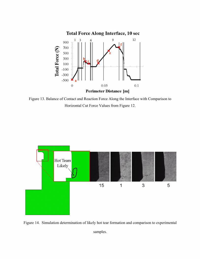
Figure 13. Balance of Contact and Reaction Force Along the Interface with Comparison to

Horizontal Cut Force Values from Figure 12.

Figure 14. Simulation determination of likely hot tear formation and comparison to experimental

samples.

References 1 Bernhard C, Xia G. Influence of alloying elements on the thermal contraction of peritectic steels during initial solidification. Ironmaking and Steelmaking, vol. 33 (1) , 2006, pp 52–56. 2. C. Bernhard, H. Hiebler and M. Wolf: Ironmaking Steelmaking, 2000, 27, 450-454. 3. C. Bernhard, W. Schutzenho¨fer, H. Hiebler and M. Wolf: Proc. 2nd Int. Conf. on ‘Science and technology of steelmaking’, April2001, Swansea, UK, 87. 4. C. Bernhard, H. Hiebler and M. Wolf: Rev. Metall., Cah. dInf.Tech., 2000, 97, 333-344. 5. P. Ackermann, J.-D. Wagniere, W.Kurz, EPFL1985, unpublished work 6. C. Bernhard, H. Hiebler, M.M. Wolf, “Simulation of Shell Strength Properties by the SSCT Test“, ISIJ Intern. 36 (1996) suppl., pp S163-S166 7. R. Pierer, C. Bernhard, C. Chimani: “A contribution to hot tearing in the continuous casting process”, La Revue de Métallurgie– CIT, February 2007, 72-83 8. C. Bernhard, H. Hiebler and M. Wolf. Simulation of Shell Strength Properties by the SSCT Test. ISIJ International, 36: 1996, pp S163-S166. 9. Reiter J., Bernhard C. & Presslinger H., Austenite grain size in the continuous casting process: Metallographic methods and evaluation, Metals Characterization, vol. 59, 2008, pp. 737-746. 10. Gigacher G., Pierer R., Wiener J. & Bernhard C., Metallurgical Aspects of Casting High-Manganese Steel Grades, Advanced Engineering Materials, vol. 8 (11), 2006, pp. 1096-1100. 11..Ackermann P., Kurz W., Heinemann W. In situ tensile testing of solidifying aluminum and Al–Mg-shells. Materials Science Engineering, vol. 75, 1985, pp. 79–86. 12. Pierer R., Bernhard C. and Chimani C. Evaluation of Common Constitutive Equations for Solidifying Steel. BHM, 150, 2005, pp. 163-169. 13. Kozlowski, P.F., Thomas, B.G., Azzi, J.A., Wang, H., Simple constitutive equations for steel at high temperature. Metallurgical and Materials Transactions, vol. 23A, 1992, pp. 903–918. 14. Zhu, H.,. Coupled thermal–mechanical finite-element modelwith application to initial solidification. Ph.D. Thesis. 1993, University of Illinois at Urbana-Champaign. 15. Wray, P.J., Plastic deformation of austenitic iron at intermediate strain rates, Metall. Trans. A, vol. 6A, 1975, pp. 1189-1196. 16. Wray, P.J., Plastic deformation of delta-ferritic iron at intermediate strain rates, Metall. Trans. A, vol. 7, 1976, pp. 1621-1627. 17. Koric, S., Thomas, B.G., Efficient thermo-mechanical model for solidification processes. International Journal for Numerical Methods in Engineering, vol. 66, 2006, pp. 1955–1989. 18. ABAQUS User Manuals v6.9 Dassault Systèmes Simulia Corp., 2009. 19. L. Hibbeler, “Thermo-Mechanical Behavior During Steel Continuous Casting in Funnel Molds”. Master’s Thesis, 2009, The University of Illinois at Urbana-Champaign. 20. K. Wiirmenberg: Stahl und Eisen, 1978, vol. 98, pp. 254-59. 21. T. Suzuki, K.-H. Tacke, and K. Schwerdtfeger: Ironmaking and Steelmaking, 1988, vol. 15, pp. 90-100. 22. Shin, G., Kajitani, T., Suzuki, T. and Umeda, T., Tetsu-to-Hagané, vol. 78, 1992, p. 587. 23. H. Mizukami, K. Nakajima, M. Kawamoto, T. Watanabe and T.Umeda: Tetsu-to-Hagané, vol, 84, 1998, p. 417. 24. H. Mizukami, S. Hiraki, M. Kawamoto and T. Watanabe: Tetsu-to-Hagané, vol. 84 (1998), 763.

25. H. Mizukami, A. Yamanaka and T. Watanabe: Tetsu-to-Hagané, vol. 85, 1999, p. 592. 26. T. Umeda, J. Matsuyama, H. Murayama and M. Sugiyama: Tetsu-to-Hagané, vol. 63, 1977, p. 441. 27. H. Suzuki, T. Nakamura and T. Nishimura: Final Report of Committee on Mechanics Related Behavior in Continuous Casting, ISIJ, Tokyo, 1985, p. 87. 28. Mizukami, H., Yamanaka, A. and Watanabe, T. High Temperature Deformation Behavior of Peritectic Carbon Steel during Solidification, ISIJ International, vol. 42 (9), 2002, pp. 964–973. 29. K. Miyazawa and K. Schwerdtfeger: lronmaking and Steelmaking,1979, pp. 68-74. 30. T. Suzuki, K.H. Tacke and K. Schwerdtfeger, “Influence of Solidification Structure on Creep Behavior of Nonalloyed Steel at High Tempertures, Met. Trans. A., 1991, vol.19A, pp. 2857-2859. 31. Sugitani, Y., Nakamura, M., Kawashima, H., Kanazawa, K., Tomono, H., and Hashio, M., Tetsu-to-Hagane´, vol. 68, 1982, pp. A149-A152. 32. Wunnenberg K. and Flender, R., Ironmaking and Steelmaking, vol. 12, 1985, pp. 22-29. 33. Nagata, S., Matsumiya T., Ozawa, K., and T. Ohashi, T. Tetsu-to-Hagane, vol. 76, 1990, pp. 214-21. 34. G. Xia, J. Zirngast, H. Hiebler and M.M. Wolf, Proceedings of the Conference on Continuous Casting of Steels in Developing Countries, The Chinese Society for Metellurgy, Beijing, 1993, p.200. 35. H. Hiebler and M.M. Wolf: CAMP-ISIJ, vol. 6, 1993, p. 1132 36. H. Hiebler, J. Zirngast, C. Bernhard and M.M. Wolf: Steelmaking Conference Proceedings, vol. 77, 1994, p. 405. 37. Hiebler H, Bernhard C. Mechanical properties and crack susceptibility of steel during solidification. Steel Research, vol. 69 (8+9), pp. 349–55. 38. Bernhard C, Hiebler H, Wolf M. Experimental Simulation of Subsurface Crack Formation in Continuous Casting. Revue Métallurgi CIT, 2000, pp. 333–344. 39. B.G. Thomas, "Modeling of Hot Tearing and Other Defects in Casting Processes," in ASM Handbook - Defects, Vol. 22, S. Viswanathan and E. DeGuire, eds., ASM, 449-461 (2008). 40. Palmaers, A., Met. Rep. CRM, No. 53, 1978, p. 23 41. Hertel, J. Litterscheidt, H., Lotter, U. And Pircher, H., Rev. Met.- CIT, vol. 89, 1992, p. 73. 42. M. Rappaz, I. Farup and J.-M. Drezet. “Study and modeling of hot tearing formation.", In Proceedings of the Merton C. Flemmings Symposium on Solidifcation and Materials Processing, pp. 213- 222 (2001). 43. M. Rappaz, J.-M. Drezet, and M. Gremaud: Metall. Mater. Trans. A, vol. 30A, pp. 449-55 (1999). 44. T.W. Clyne T.W. and G.J. Davies: Solidification and Casting of Metals, Metals Society, London, pp. 275-78 (1979). 45. U. Feurer: in Quality Control of Engineering Alloys and the Role of Metals Science, H. Nieswaag and J.W. Schut, eds., Delft University of Technology, Delft, The Netherlands, 1977, pp. 131-45. 46. L. Katgerman, J. Met., vol. 34 (2), pp. 46-49 (1982). 47. D.G. Eskin, and L Katgerman,., “A Quest for a New Hot Tearing Criterion”, Metallurgical and Materials Transactions A, Vol. 38(A) , 1511-1519 (2007). 48. B. Magnin, L. Maenner, L. Katgerman, and S. Engler: Mater. Sci. Forum, vols. 217–222, pp. 1209-14 (1996).

49. L. Zhao, Baoyin, N.Wang, V. Sahajwalla, and R.D. Pehlke: Int. J. Cast Met. Res., vol. 13 (3), pp. 167-74 (2000). 50. Y.M. Won, T.J. Yeo, D.J. Seol and K.H. Oh, “A new criterion for internal crack formation in continuously cast steels”,Met. Trans. B, vol. 31B, pp.779-794 (2000). 52. M. Braccini, C.L. Martin, M. Sue´ry, and Y. Bre´chet: in Modelling of Casting, Welding and Advanced Solidification Processes IX, P.R. Sahm, P.N. Hansen, and J.G. Conley, eds., Shaker Verlag, Aachen, Germany, 2000, pp. 18-24. 53. N.N. Prokhorov: Russ. Castings Production, No. 2, pp. 172-75 (1962). 54. E. Niyama: in Japan–US Joint Seminar on Solidification of Metals and Alloys, Japan Society for Promotion of Science, Tokyo, pp. 271-82 (1977). 55. J.F. Grandfield, D.J. Cameron, and J.A. Taylor: in Light Metals 2001, J.L. Anjier, ed., TMS, Warrendale, PA, pp. 895-901 (2001). 56. J.-M. Drezet and M. Rappaz: in Light Metals 2001, J.L. Anjier, ed., TMS, Warrendale, PA, pp. 887-93, (2001). 57. C.H. Dickhaus, L. Ohm, and S. Engler: Trans. Am. Foundrymen’s Soc., vol. 101, pp. 677-84, (1994). 58. J. Langlais and J.E. Gruzleski: Mater. Sci. Forum, vols. 331-37, pp. 167-72, (2000). 59. D.J. Lahaie and M. Bouchard: Metall. Mater. Trans. B, vol. 32B, pp. 697-705 (2001). 60. J.A. Williams and A.R.E. Singer: J. Inst. Met., vol. 96, pp. 5-12, (1968). 61. Rogberg, B., An Investigation on the hot ductility of steels by performing tensile tests on In situ solidified samples, Scand.J. Metall., vol. 12, 1983, pp.51-66. 62. Suzuki, M., M. Suzuki, C. Yu and T. Emi. “In-situ measurement of fracture strength of solidifying steel shells to predict upper limit of casting speed in continuous caster with oscillating mold." ISIJ International 37(4), 375-382 (1997). 63. Yavari, P., Miller, D.A. and Langdon, T.G., An investigation of Harper-Dorn creep, I, Mechanical and microstructural characteristics, Acta Metall., vol. 30, 1982, pp. 871-879. 64. Clyne, T.W., Davies, G.J., The influence of composition on solidification cracking susceptibility in binary alloy systems, ,Br. Foundryman, vol. 74,1981, pp. 65-73. 65. Weiner, J.H., Boley, B.A., Elastic–plastic thermal stresses in a solidifying body. Journal of the Mechanics and Phyics of Solids, vol. 11, 1963, 145–154. 66. Grill, A., Brimacombe, J.K., Weinberg, F., Mathematical analysis of stress in continuous casting of steel. Ironmaking and Steelmaking, vol. 3, 1976, pp. 38–47. 67. Wimmer, F., Thone, H., Lindorfer, B., Thermomechanically-coupled analysis of the steel solidification process in continuous casting mold. ABAQUS Users Conference, 1996. 68. Rammerstrofer, F.G., Jaquemar, C., Fischer, D.F., Wiesinger, H., Temperature Fields, Solidification Progress and Stress Development in the Strand During A Continuous Casting Process of Steel, Numerical Methods in Thermal Problems., Pineridge Press, 1979 ed., pp. 712–722. 69. Kristiansson, J.O., Thermomechanical behavior of thesolidifying shell within continuous casting billet molds—a numerical approach. Journal of Thermal Stresses, vol. 7, 1984, pp. 209–226. 70. Boehmer, J.R., Funk, G., Jordan, M., Fett, F.N., Strategies for coupled analysis of thermal strain history during continuous solidification processes. Advanced Software Engineering, vol. 29 (7–9), 1998, pp. 679–697. 71. Farup, I., Mo, A., Two-phase modeling of mushy zone parameters associated with hot tearing. Metallurgical and Materials Transactions, vol. 31, 2000, pp. 1461–1472.

72. Li, C., Thomas, B.G., Thermo-mechanical finite-element model of shell behavior in continuous casting of steel. Metallurgical and Materials Transactions B, vol. 35B (6), 2005, pp. 1151–1172. 73. Risso, J.M., Huespe, A.E., Cardona, A., Thermal stress evaluation in the steel continuous casting process. International Journal for Numerical Methods in Engineering, vol. 65 (9), 2006, pp.1355–1377. 74. Bernhard C., Pierer R., Tubikanec A. And Chimani C.M. Experimental Characterization of Crack Sensitivity under Continuous Casting Conditions, CCR, Continuous-Casting Innovation Session, paper no. 06.03, 2004, pp. 1-9. 75. Bernhard C. & Pierer R., High Temperature Behavior During Solidification of Peritectic Steels under Continuous Casting Conditions, MS&T, 2006. 76. Kurz W., About Initial Solidification in Continuous Casting of Steel, La Metallurgia Italiana, Lugio/Agosto, 2008, pp. 56-64. 77. Seid Koric, Lance C. Hibbeler, and Brian G. Thomas, “Explicit Coupled Thermo-Mechanical Finite Element Model of Steel Solidification”, International Journal for Numerical Methods in Engineering, vol. 78, 2009, pp. 1-31. 78.Li, C., Thermal-Mechanical Model of Solidifying Steel Shell Behavior and Its Applications in High Speed Continuous Casting of Billets. Ph.D. Thesis, 2004, The University of Illinois at Urbana-Champaign. 79.Y. Meng and B.G. Thomas, Heat Transfer and Solidification Model of Continuous Slab Casting: CON1D, Metallurgical and Materials Transactions B, 34 (B5), 2003, pp. 685-705. 80.Harste, K., Investigation of the shrinkage and the origin of mechanical tension during solidification and successive cooling of cylindrical bars of Fe–C alloys. Ph.D. Thesis. 1989, Technical University of Clausthal. 81. Harste, K., A. Jablonka and K. Schwerdtfeger. Shrinkage and formation of mechanical stresses during solidification of round steel strands." In 4th International Conference Continuous Casting, D.-. D. . F. Verlag Stahleisen, Vol. 2, pp. 633-644. 82. Jimbo, I. and A. A. W. Cramb. The density of liquid iron carbon alloys. Metallurgical and Materials Transactions B. 24B (1), 1993, pp. 5-10. 83. Mizukami, H., K. Murakami and Y. Miyashita. Elastic modulus of steels at high temperature." Tetsu-to-Hagane, 63 (146), S652 (1977). 84. Won Y.M. and Thomas B.G., Simple Model of Microsegregation during Solidification of Steels, Metallurgical and Materials Transactions. A, vol. 32 (A), 2003, pp. 1755-1767. 85. A.M. Lush, G. Weber and L. Anand, An implicit time–integration procedure for a set of integral variable constitutive equations for isotropic elasto-viscoplasticity, International Journal of Plasticity 5 (1989) 521-549.

Appendices

Appendix A – SSCC Test Simulation Dimensions

Figure A-1. SSCC Dimensions (mm)

Appendix B – Material Properties of Steel Melt and SSCC Test Body

Figure B-2. Phase Fractions for SSCC PP05

The temperature dependent thermal conductivity (below) was taken from Harste and Jablonka

[80, 81] and Jimbo and Cramb [82]

[ ]

[ ]

2

2

α α γ γ δ δ l l

2 a2 o 5 oα 1

3 oγ

a3 oδ 1

l

4 o1

2

k[W/m/K] k f k f k f k f

k 80.91 9.9269 10 T C 4.613 10 T C 1 a %C

k 21.6 8.35 10 T C

k 20.14 9.313 10 T C 1 a %C

k 39.0

a 0.7425 4.385 10 T C

a 0.20

− −

−

−

−

= + + +

= − × + × − = − × = − × −

=

= − ×

= 3 o9 1.09 10 T C− + ×

(A-1)

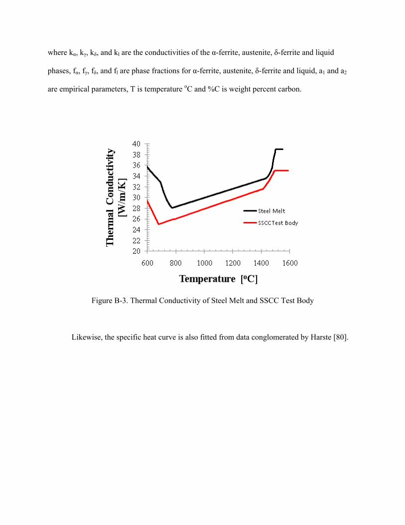
where kα, kγ, kδ, and kl are the conductivities of the α-ferrite, austenite, δ-ferrite and liquid

phases, fα, fγ, fδ, and fl are phase fractions for α-ferrite, austenite, δ-ferrite and liquid, a1 and a2

are empirical parameters, T is temperature oC and %C is weight percent carbon.

Figure B-3. Thermal Conductivity of Steel Melt and SSCC Test Body

Likewise, the specific heat curve is also fitted from data conglomerated by Harste [80].

[ ]( )[ ]( )

[ ]

[ ]( ) [ ][ ]( ) [ ]

[ ]( )[ ]( )

p p α α p,γ γ p,δ δ p l l

3

2

p α

2

c [J/kg] c , f c f c f c , f

5217657 1010068.18 5.98686 T K , T K 1060

T K

34871.21 32.02658 T K , 1042 T K ,1060

11501.07 12.476362 T K , 1000 T K 1042c ,

11094834720.324 4.583364 T K

T K

= + + +

× − + × + >

− × <

− + × < <=

− + × +

[ ]

[ ]( )[ ]( )

[ ]( )( ) [ ]

( )

[ ]( )[ ]( )

2

2

p δ

p γ

p l

A 2

, 800 T K 1000

5187583.4504.8146 0.1311139 T K 0.000448666 T K , T K 800

T K

c , 441.3942 0.17744236 T K

c , 429.8495 0.1497802 T K

c , 824.6157

− < < − × + + + <

= + ×

= + ×

=

Where cp,α, cp, γ, cp, δ, and cp,l is the specific heat of the α-ferrite, austenite, δ-ferrite and liquid

phases respectively and T is temperature in K.

The latent heat, Lf, was assumed to be 271,000 J/kg. The effective specific heat, *pc , is

used to distribute the latent heat in the mushy zone according to the increase in the solid fraction,

fs as the shell cools from the liquidus to the solidus temperature according to eq. (A-3)

dT

dfLcc s

fpp −=* (A-3)

Figure B-4. Specific Heat of Steel Melt and SSCC Test Body

The thermal linear expansion (TLE) is determined from solid phase density measurements of

Harste [80] and Jablonka [81] and by Jimbo and Cramb [82] for liquid steels. Equations for both

TLE and density are given in eq. (4).

[ ] ( )( )

( )( )

( )( ) ( )( )( )

( )( ) ( )( )( ) ( )( ) ( )( )

3

3

25

3

3

1

where

7881 0.324 3 10

100 8106 0.51

100 % 1 0.008 %

100 8011 0.47

100 % 1 0.013 %

7100 73 % 0.8 0.09 % 1550

ref

l l

o o

o

o

ol

TTLE

T

kg f f f fm

T C T C

T C

C C

T C

C C

C C T C

α α γ γ δ δ

α

γ

δ

ρρ

ρ ρ ρ ρ ρ

ρ

ρ

ρ

ρ

−

− = −

= + + +

= − − ×

− =− +

− =− +

= − − − −

(A-4)

where TLE is the thermal linear expansion, ρα, ργ , ρδ, and ρl are the densities kg/m3 of the α-

ferrite, austenite, δ-ferrite and liquid phases and T is temperature oC. The TLE is converted to a

thermal expansion coefficient, α, by computing the slope of the TLE vs. temperature curve. The

reference temperature was chosen to be 300 oC with a reference TLE of -1.66 x 10-2.

( )ref

oref

TLE TLE T1α

T TC

− = − (A-5)

Figure B-7. Density of Steel Melt and SSCC Test Body

The elastic modulus used is a function of data obtained by Mizukami [83].

Figure B-8. Elastic Modulus

Appendix D – Zirconium Oxide Material Properties

Specific Heat J/kg/K Temperature oC

100 0

100 300

100 800

100 1000

100 1500

Thermal Conductivity W/m/K Temperature oC

2.72 400

2.26 800

2.2 1200

Density kg/m3 Temperature oC

3030 300

3010 800

2990 1000

2940 1500

Elastic Modulus = 300 GPa

Poisson’s Ratio = 0.3 [-]

Thermal Expansion Coefficient = 12 x 10-6 1/ oC, reference temperature = 25 oC