Measuring impacts and adaptations to climate change: a ...huardda/articles/seo08.pdf · AGRICULTURAL ECONOMICS Agricultural Economics 38 (2008) 151–165 Measuring impacts and adaptations

AGRICULTURALECONOMICS

Agricultural Economics 38 (2008) 151–165

Measuring impacts and adaptations to climate change: a structural Ricardianmodel of African livestock management1

S. Niggol Seoa,∗, Robert Mendelsohnb

aWorld Bank, 8508 16th Street, Suite 302, Silver Spring, MD 20910, USAbSchool of Forestry and Environmental Studies, 230 Prospect St., New Haven, CT 06511, USA

Received 29 April 2007; received in revised form 15 August 2007; accepted 15 August 2007

Abstract

This article develops a new cross-sectional methodology that explicitly incorporates adaptation into an analysis of the impacts of climate change.The methodology examines how a farmer will change choices of species and number to adapt to climate. The approach is applied to study Africa,where the impacts of climate change are expected to be the most severe. The results indicate that in warmer places, African farmers switch frombeef cattle to more heat-tolerant goats and sheep. In wetter places, farmers switch from cattle and sheep to goats and chickens. The results indicatethat large commercial livestock operations specializing in beef cattle will be hard hit from climate change whereas small farmers who can easilysubstitute to goats and/or sheep will be more resilient.

JEL classification: C53, O13, O18, O55, R11

Keywords: Climate change; Africa; Livestock; Cross-sectional adaptation analysis

1. Introduction

This article uses cross-sectional evidence to explore howfarmers adapt to exogenous environmental factors such as cli-mate and soils. The model builds on the original insights ofthe Ricardian model that explored the locus of land valueper hectare (Mendelsohn et al., 1994). Although the Ricardianmodel captures adaptation in its measure of impacts, it doesnot provide any insight into how farmers adapt. In this arti-cle, we develop a new approach, a Structural Ricardian Model,that explicitly models the underlying endogenous decisions byfarmers. By comparing choices of farmers who face differentconditions, the model uncovers how farmers adapt. Conditionalincomes, using a Ricardian approach, are then estimated foreach choice made by each farmer.

∗Corresponding author: Tel.: 203-432-9771. Fax: 203-432-3809.

E-mail address: [email protected] (S. Niggol Seo).1The authors wish to thank the World Bank and Global Environment Facility

for funding and the Center for Environmental Economics and Policy in Africaat the University of Pretoria for their overall management of this project. Weare especially thankful to Ariel Dinar at the World Bank, Rashid Hassan atCEEPA, and Pradeep Kurukulasuriya at UNDP. We would also like to thankProfessors Robert Evenson, Donald Andrews, Daniel Esty, and Erin Mansurat Yale University, Professor Kenneth Train at the University of California atBerkeley, many seminar participants at Yale University and Purdue University,and two anonymous reviewers for their valuable comments.

We develop this new method and then apply it to study howAfrican farmers adapt livestock management to climate. Weexplore which species they choose, how many animals theyown, and how net revenue per animal for each species changes.Understanding adaptation is an important goal in itself to assistplanning by policy makers and private individuals. However,understanding adaptation is also important if one is interestedin quantifying the impacts of climate change. Forecasts thatover- or underpredict adaptation will under- or overpredict theresidual damages from climate change.

Climate impact studies have consistently predicted extensiveimpacts to the agricultural sector from climate change acrossthe globe (Pearce et al., 1996; McCarthy et al., 2001; Tol, 2002).The bulk of agricultural studies on the effect of climate changehave focused on crops. However, a large fraction of agriculturaloutput is from livestock. In the United States, livestock accountfor about 40% of the market value of agricultural products sold(USDA, 2002). Almost 80% of African agricultural land is usedfor grazing. Yet there are very few economic analyses of cli-matic effects on livestock. An important exception is the studyof the effects of climate change on American livestock (Adamset al., 1999). American livestock appear not to be vulnerableto climate change because most live in protected environments(sheds, barns, etc.) and rely heavily on supplemental feed (e.g.,hay and corn). African livestock have no protective structuresand they graze off the land. As a result, we anticipate that

c© 2008 International Association of Agricultural Economists

152 S. N. Seo, R. Mendelsohn / Agricultural Economics 38 (2008) 151–165

Profit

Temperature

All Livestock Species 1 Species 2 Species 3

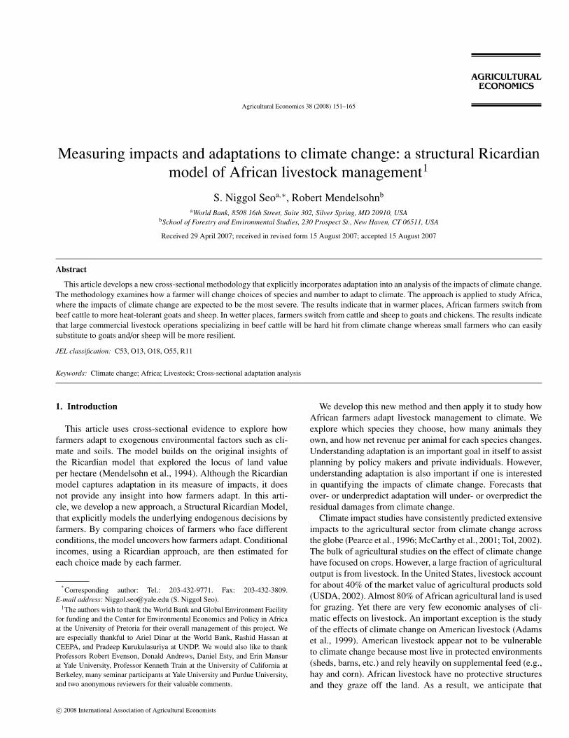
Fig. 1. Theoretical livestock response functions.

African livestock will be sensitive to climate change. In a sepa-rate article, the Ricardian model is applied to African livestockdata (Seo et al., 2007) and shows that livestock are sensitiveto climate. In this article we provide insight into how farmersadjust to climate and what they might do in the future.

The underlying theory of the Structural Ricardian Model isdeveloped in the next section. Section 3 discusses how datawere collected from over 5,000 farmers who own livestock in10 countries across Africa for this study. Section 4 discussesthe estimation procedure and the cross-sectional empirical re-sults. Forecasted impacts from three climate change scenariosgenerated by Atmospheric Oceanic General Circulation Mod-els (AOGCMs) are then examined in Section 5. The articleconcludes with a summary of results and policy implications.

2. Theory

A farmer’s optimization decision can be seen as a simulta-neous multiple-stage procedure. The farmer chooses the levelsof inputs, the desired number of animals, and the species thatwill yield the highest net profit. Given the profit-maximizinginputs from each farmer, one can estimate the loci of profit-maximizing choices for each species across exogenous envi-ronmental factors such as temperature or precipitation. Theseare the individual loci that lie beneath the overall profit functionfor the farm (Mendelsohn et al., 1994). We call the approacha “cross-sectional adaptation model” because it estimates thechoice of a specific animal, the number of animals, and the un-derlying profit response functions per animal for each species

that form the overall profit function. For example, in Fig. 1we display a traditional Ricardian response function with re-spect to temperature. Underneath the locus of all choices is aset of species-specific response functions. Given the climate,the farmer must choose the most profitable species and also theinputs that will maximize the value of that species. We examinethe individual net revenue functions for each species as well asthe overall net revenue function across all species. We assumethat each farmer makes his animal husbandry decisions to max-imize profit.2 Hence, the probability that a species is chosendepends on the profitability of that animal species (or crop ifone wants to examine the crop sector). We assume that farmeri’s profit in choosing livestock j (j = 1, 2, . . . , J) is

πji = V (Zji) + εji, (1)

where Z is a vector of independent variables that includes cli-mate variables, soils, and other socioeconomic variables suchas household characteristics. The profit function in Eq. (1) iscomposed of two components: the observable component V andan error term ε. The error term is unknown to the researcher, butmay be known to the farmer. The farmer will choose the live-stock that gives him the highest profit. The farmer will choose

2 The theory of profit maximization can be contested especially in Africa (DeJanvry et al., 1991; Moll, 2005; Singh et al., 1986). We made the following twoadjustments to address the issues arising from special situations of African mar-kets. First, we assume that if a farmer consumes his own product, it is valued atmarket price. Second, most farms depend on their own labor. Although it mightbe reasonable to value own labor by market wages, empirical examinations didnot support any specific wage.

S. N. Seo, R. Mendelsohn / Agricultural Economics 38 (2008) 151–165 153

animal j over all other animals if

π∗(Zji) > π∗(Zki) for ∀k �= j

× [or if εk − εj < V (Zji) − V (Zki) for k �= j]. (2)

More succinctly, farmer i’s problem is

arg maxj

[π∗(Z1i), π∗(Z2i), . . . , π

∗(ZJi)]. (3)

The probability Pji for the jth livestock to be chosen is then

Pji = Pr[εk − εj < Vj − Vk] ∀k �= j where Vj = V (Zji). (4)

Assuming ε is independently and identically Gumbel dis-tributed3 and Vk can be written linearly in the parameters

Pji = exp(Zjiγj )∑Jk=1 exp(Zkiγk)

, (5)

which gives the probability that farmer i will choose livestockj among J animals (Chow, 1983; McFadden, 1981).

The parameters can be estimated by the maximum likeli-hood method using an iterative nonlinear optimization tech-nique such as the Newton–Raphson method. These estimatesare CAN (Consistent and Asymptotically Normal) under stan-dard regularity conditions (McFadden, 1999).

Note that farmers can choose more than one species of live-stock among the five species in our study. That is, there are manycombinations of livestock species that the farmer could choose.In this analysis, we assume that farmers choose one primaryspecies from the five species. A primary species is defined asthat which generates the highest total net revenue for the farm(Train, 2003). In another analysis of livestock choice, we com-pare this approach using the primary species with an alternativeportfolio approach that examines all possible choices includingcombinations of species (Seo and Mendelsohn, 2007). The twoapproaches yield similar results.

Conditional on the livestock species chosen, we estimate theoptimal number of animals per farm for each species and thenet revenue per animal for each species. We rely on a two-stagemodel. In the first stage, we estimate the probability of selectinga species (Eq. 5). In the second stage, conditional on the choiceof a specific species, we estimate the optimal number of thatspecies and the net revenue per animal. We identify the specieschoice equations using the relative prices of each choice. Weidentify the number of animal equations using the percentageof grassland in the district. Note that this more general variablewas used instead of grassland on the farm because many Africanlivestock owners graze animals on common lands.

3 Two common assumptions about the error term are either the Normal orthe Gumbel distribution. Normal random variables have the property that anylinear combination of normal varieties is normal. The difference between twoGumbel random variables has a logistic distribution, which is similar to thenormal but with larger tails. Thus the choice is somewhat arbitrary with largesamples (Greene, 1998).

Because the profit described in Eq. (1) is observed only forthe chosen species, one must correct for possible selection biaswhen estimating the conditional net revenues or numbers ofanimals (Heckman, 1979). Since the farmer maximizes net rev-enue conditional on the choice of that species, the error in thesecond-stage equation may be correlated with the error in thefirst stage. According to Dubin and McFadden (1984), with theassumption of the following linearity condition4:

E(uj |ε1, . . . , εJ ) = σ ·J∑

j=1

rj · (εj − E(εj )), withJ∑

j=1

rj = 0,

(6)

where uj is the error from the profit equation in the secondstage, εj is the error from the choice equation in the first stage,σ is the standard error of the profit equation, and rj the corre-lation between the profit equation and choice equations, thenthe selection bias-corrected conditional profit functions can beconsistently estimated as

πj = Xjϕj + σ ·J∑

i �=j

ri ·(

Pi · ln Pi

1 − Pi

+ ln Pj

)+ wj, (7a)

where the second term on the right-hand side is the selectionbias correction term; Xj is a set of independent variables thatinclude climate variables, soils, and socioeconomic variables;ϕj is a vector of parameters; and wj is the error term.

The optimal number of animals can be estimated in the samemanner:

Nj = Xjηj + σ ·J∑

i �=j

ri ·(

Pi · ln Pi

1 − Pi

+ ln Pj

)+ vj , (7b)

where the various terms are defined similarly as in Eq. (7a).The two-stage model is composed of Eq. (5) and equations

(7a) and (7b). Expected net revenue is therefore

Wi(Zi) =J∑

j=1

Pj (Zji) · πj (Zji) · Nj (Zji). (8)

Because climate is an independent variable in all three termsin Eq. (8), the marginal effect on welfare of a change in aclimate variable, say Zc, has three components: the effect on theprobability of the livestock to be chosen, the direct effect on theconditional profit per animal, and the effect on the conditionalnumber of animals:

∂Wj

∂zc

= ∂Pj

∂zc

· πj · Nj + ∂πj

∂zc

· Pj · Nj + ∂Nj

∂zc

· Pj · πj , (9)

4 See Bourguignon et al. (2004) for the details of the selection bias correc-tions from the multinomial choice. They find that in most cases, Dubin andMcFadden’s method is preferable to the most commonly used Lee method,as well as to Dhal’s semiparametric method. Monte Carlo experiments showthat selection bias correction based on the multinomial logit model can providefairly good correction for the outcome equation even when the IIA hypothesisis violated.


where the marginal effect on the probability can be obtained bydifferentiating Eq. (5):

∂Pj

∂zc

= Pj

[γj −

J∑k=1

Pkγk

], (10)

and the marginal effect on the net revenue per animal, assuminga quadratic relationship between the net revenue and the cor-responding climate variable, can be obtained by differentiatingEq. (7a):

∂πj

∂zc

= ϕj1 + 2 · ϕj2 · zc, (11)

and the marginal effect on the number of animals per farm,also assuming a quadratic relationship between the number ofanimals and the relevant climate variable, can be found bydifferentiating Eq. (7b):

∂Nj

∂zc

= ηj1 + 2 · ηj2 · zc, (12)

where the subscripts 1 and 2 in equations (11) and (12) denotethe estimated parameters for the linear term and the quadraticterm for the climate variable zc.

The change in welfare resulting from a nonmarginal changein climate can be computed as the difference in the expectednet revenues in the two states before and after climate change.Suppose that climate changes from Cbefore to Cafter. Then thechange in welfare can be approximated as

Wi = Wi(Cafter) − Wi(Cbefore). (13)

The uncertainty surrounding our measure of the welfarechange can be described by the 95% confidence interval ofthe expected climate change impact. In principle, there are twoways to calculate confidence intervals: parametric and non-parametric. It is difficult to calculate the variance of the climatechange impact parametrically in this model because welfare isthe product of three predictions. We provide uncertainty esti-mates in this study via a bootstrap method by resampling 200times from the original sample and calculating the 95% con-fidence interval using the mean and the standard deviation ofthe resulting climate change impacts (Andrews and Buchinsky,2000).

3. Data

Data for this study come from a larger Global Environmen-tal Facility (GEF)–World Bank project to study climate changeimpacts on agriculture in Africa (Dinar et al., 2008). The coun-tries included were Burkina Faso, Cameroon, Egypt, Ethiopia,Ghana, Kenya, Niger, Senegal, South Africa, and Zambia. (Zim-babwe had to be dropped from the livestock analysis becauseof turbulent conditions in that country during the survey.) The

countries were selected to represent the wide range of climatethroughout Africa. Districts within each country were selectedto provide as much within-country climate variation as possible.Because existing economic data were not sufficient to supportan analysis, an economic survey of farmers was conducted. Theoriginal survey interviewed more than 9,000 farmers from 11countries. Within that sample, more than 5,000 were livestockfarmers (Kurukulasuriya et al., 2006).

The livestock data include information on species, the stockof livestock owned, and the livestock products and animalssold during the period of July 2002 to June 2003 (the datafrom Kenya, Ethiopia, and Cameroon cover the period July2003 to June 2004). The data identify the five major types oflivestock in Africa as beef cattle, dairy cattle, goats, sheep,and chickens. Other less frequently recorded animals includepigs, breeding bulls, oxen, camels, ducks, guinea fowl, horses,bees, and doves. The major livestock products sold were milk,meat, eggs, wool, and leather. Other products included butter,cheese, honey, skins, and manure. The five major livestockaccounted for 93% of the total net livestock revenue in thesample (Seo and Mendelsohn, 2007).

All countries in the sample had a large number of livestockfarms. Most of the farms in our survey were small householdfarms, but a majority of the farms in South Africa and Kenya lo-cated in temperate climate zones were large commercial farms.Definitions of what constitutes a small household farm versusa large commercial farm are country-specific. South Africa hada large number of commercial beef cattle farms while Kenyanfarmers kept dairy cattle and beef cattle in large numbers. Farm-ers in Egypt tended to raise chickens while West African farm-ers depended more on goats and sheep (Seo and Mendelsohn,2007).

Climate data come from two sources: U.S. Defense Depart-ment satellites and weather station observations. We relied onsatellite temperature observations and interpolated precipita-tion observations from ground stations (see Mendelsohn et al.[2007] for a detailed explanation). The climate data measuresthe long-run average weather (17 to 30 years), not the weatherin the particular year of the economic survey. Climate datawere gathered in monthly measures of temperature (◦C) andprecipitation (mm/month) and then aggregated by season: Win-ter (May, June, July), Spring (August, September, October),Summer (November, December, January), and Fall (February,March, April). Seasons for locations north of the equator weredefined in reverse. Soil data were obtained from the FAO dig-ital soil map of the world (Food and Agriculture Organization[FAO] 2004). Soil data were extrapolated to the district levelusing GIS. The data set reports 116 dominant soil types and 26aggregated soil types.

4. Empirical results

As indicated above, although there are many livestockspecies in Africa, we focus on the five primary species that


Table 1Multinomial logit species selection model

Beef cattle Dairy cattle Goats Sheep

Variable Estimate χ2 Odds ratio Estimate χ2 Odds ratio Estimate χ2 Odds ratio Estimate χ2 Odds ratio

Intercept 5.94 5.58 10.85 45.7 −0.22 0.01 4.92 6.85Temperature summer 0.31 2.82 1.37 −0.942 76.5 0.39 −0.168 1.74 0.85 −0.105 0.68 0.90Temperature summer sq −0.0047 1.62 1.00 0.0157 53.3 1.02 0.0049 3.79 1.01 0.0023 0.83 1.00Precipitation summer 0.0058 0.94 1.01 −0.0201 27.6 0.98 −0.0119 8.54 0.99 −0.0155 12.7 0.99Precipitation summer sq 0.0000 0.22 1.00 0.0001 12.6 1.00 0.0001 14.4 1.00 0.0000 3.03 1.00Temperature winter −1.18 73.7 0.31 0.296 5.41 1.35 0.0755 0.16 1.08 −0.435 8.63 0.65Temperature winter sq 0.0284 52.6 1.03 −0.0036 1.17 1.00 0.0003 0.00 1.00 0.0139 12.07 1.01Precipitation winter 0.020 5.53 1.02 0.0065 1.44 1.01 −0.0178 8.98 0.98 −0.0243 14.5 0.98Precipitation winter sq −0.0001 1.52 1.00 −0.0001 5.98 1.00 0.0001 5.07 1.00 0.0000 0.22 1.00Soil Cambisols 1.09 1.30 2.97 1.59 7.04 4.93 0.503 0.79 1.65 0.6404 1.33 1.90Soil Gleysols −1.86 1.17 0.16 −7.35 25.1 0.00 −2.63 4.23 0.07 −3.67 5.90 0.03Electricity 0.96 18.3 2.60 −0.078 0.19 0.93 0.0658 0.16 1.07 0.336 4.23 1.40Beef cattle price −0.0027 10.06 1.00 0.0002 0.07 1.00 −0.0016 3.32 1.00 −0.0033 16.1 1.00Milk price −0.482 11.25 0.62 0.511 24.4 1.67 0.0489 0.20 1.05 −0.0323 0.09 0.97Goat price 0.0212 5.10 1.02 0.0136 3.92 1.01 −0.0180 3.90 0.98 −0.0261 8.31 0.97Sheep price 0.0066 1.85 1.01 0.0034 0.79 1.00 −0.0085 2.57 0.99 −0.0037 0.53 1.00Chicken price −0.513 14.4 0.60 −1.074 142 0.34 0.416 18.9 1.52 0.765 66.5 2.15

Notes: (1) The base case is chickens.(2) The critical value of chi-square statistic for the significance at 5% is 3.7.(3) Three tests of global significance of the model: Likelihood ratio test: P < 0.0001, Lagrange multiplier test: P < 0.0001, and Wald test: P < 0.0001.

generated the most livestock income: beef cattle, dairy cat-tle, goats, sheep, and chickens.5 We model the probability ofchoosing each species as a function of summer and winter tem-perature and summer and winter precipitation. We also includeother explanatory variables such as dominant soils and a dummyvariable for electricity. We identified the selection equations bythe input and output prices of the five species. For example, thehigher the price of milk (one of the primary outputs) the morelikely farmers are to choose dairy cattle and goats, but the lesslikely they are to choose sheep and beef cattle.

Table 1 shows the results of the multinomial logit regressionof the probability of choosing each of the five species. The basecase is a household that chose chickens. Most of the coefficientestimates are significantly different from zero. The three testsof the global significance of the model—likelihood ratio test,Lagrange multiplier test, and Wald test—verify that the modelis highly significant. The coefficients report the odds ratio. Forexample, the odds ratio of the electricity dummy for beef cattleis 2.6, which implies that farms with electricity are 2.6 times(odds ratio) more likely to own beef cattle than farms withoutelectricity. Farms with electricity are also more likely to choosesheep but less likely to choose dairy cattle and goats. Soil vari-ables are weakly significant and their coefficients vary acrosslivestock species. For example, dairy cattle are more likely tobe chosen under Cambisol soils, but not under Gleysol soils.Under Gleysol soils, beef cattle are more likely to be selected,compared with other species.

5 Species can be further differentiated by breeds (Oklahoma State University,2007). For example, some breeds of beef cattle and sheep are more heat tolerantthan others. Information about breeds was not collected in the survey and sothis study does not distinguish between different breeds within species.

Coefficients for livestock prices are significantly differentfrom zero in most cases. As the price of milk, the primary out-put from dairy cattle and goats, rises, more farmers choose dairycattle and goats. Own animal price was difficult to interpret be-cause it is both the price of buying an animal (input price) andthe price of selling it (output price). In general, higher ownprices led farmers away from choosing a species. For example,higher beef cattle prices discouraged farmers from selectingbeef cattle. Cross price effects are also evident in Table 1. Neg-ative cross price terms imply that two animals are incompatiblewhereas positive cross price terms imply that they can be raisedjointly. For example, the coefficient on the price of goats (chick-ens) is positive (negative) for beef and dairy cattle but negative(positive) for sheep, implying that goats (chickens) can be raisedwith cattle (sheep) but not sheep (cattle).

Most climate variables are significantly different from zero.The quadratic summer temperature coefficients are positive forgoats, sheep, and dairy cattle implying a U-shaped functionbut the temperature response function for beef cattle is hill-shaped. The quadratic coefficients of the precipitation variablesare generally positive, indicating a U shape except for beef cattleand dairy cattle responses to winter precipitation. Althoughnot shown in Table 1, we also tested for the effects of otherimportant control variables such as water availability, altitude,and other social factors such as religion. These variables weredropped because they were not significant. We also tested anumber of variables describing the farmer including gender,age, and education but these too were not significant and sowere dropped.

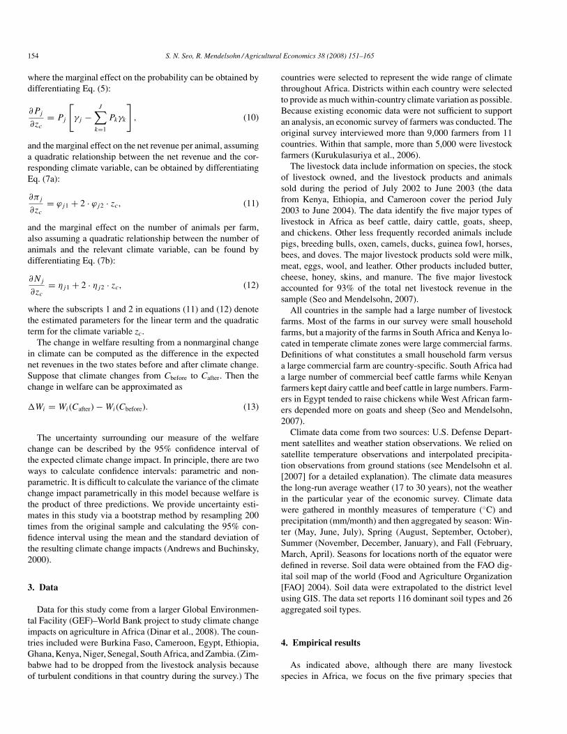
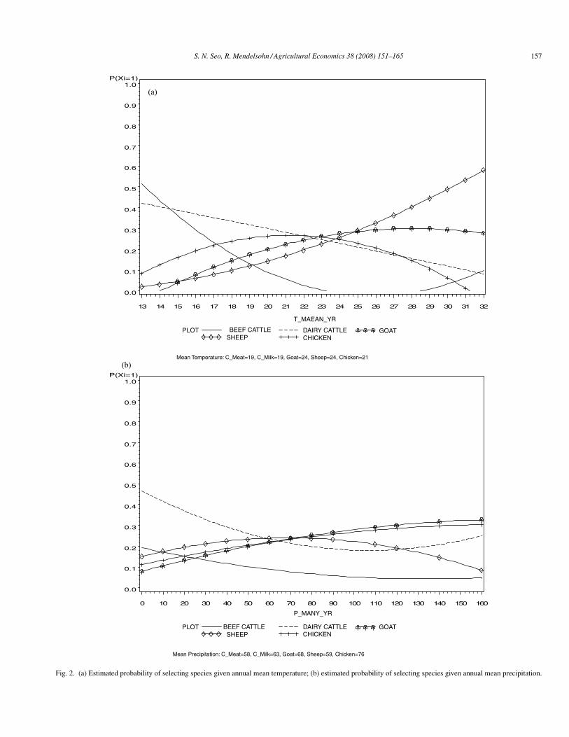
Fig. 2a graphs the relationship between the probability ofchoosing a species and annual temperature. Note that the meantemperature in sub-Saharan Africa is 22◦C. The probability of


choosing beef cattle and dairy cattle decreases rapidly as tem-perature rises. In contrast, the probability of choosing goats andsheep climbs as temperature rises. With chickens, the estimatedprobability is hill-shaped, with a maximum at the current meantemperature of Africa. The graph clearly reveals that farmersin Africa today choose animal species selectively to make thebest use of the current temperature.

Fig. 2b displays the estimated relationship between the prob-ability of choosing a species and annual precipitation. Theprobability of choosing beef cattle, dairy cattle, and sheep alldecreases as precipitation increases. Greater rainfall increasesthe probability of diseases such as Trypanosomiasis (Nagana),Theileriasis (East Coast Fever), and Rift Valley Fever (Fordand Katondo 1977; University of Georgia, 2007) and, perhapsmore importantly, in the long term, shifts the ecosystem fromsavanna to forest (Sankaran et al., 2005). All three of the largegrazing animals are clearly more productive in grasslands. Incontrast to the above results, goats and especially chickens aremore likely as rainfall increases. Goats may be relatively betterable to forage successfully in forest settings.

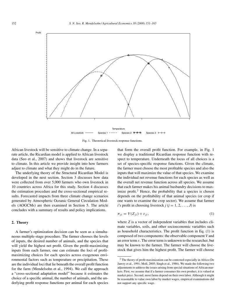
In the second stage of the analysis, we estimate the condi-tional net revenue functions. The net revenue per animal foreach chosen species is regressed on climate variables, soil vari-ables, a dummy variable for electricity, and sale price of thecorresponding livestock. We identify these net revenue regres-sions by the sale prices. We account for selection bias by usingthe Dubin–McFadden selection bias correction terms. Theseconditional net revenue regressions use the same seasonal cli-mate variables used in the choice regressions. The functionalform is quadratic in both temperature and precipitation.

Table 2Conditional net revenue per animal regression

Beef cattle Dairy cattle Chickens Goats Sheep

Variable Estimate T-statistic Estimate T-statistic Estimate T-statistic Estimate T-statistic Estimate T-statistic

Intercept 280 0.90 6.83 0.04 3.92 1.19 −17.1 −0.45 69.3 2.82Temp summer 63.3 2.35 −7.98 −0.53 0.621 2.66 −5.35 −2.04 3.47 1.84Temp summer sq −1.15 −2.37 0.300 1.11 −0.010 −2.16 0.119 2.54 −0.041 −1.16Temp winter −143 −6.22 0.639 0.04 −1.29 −4.81 7.13 1.88 −10.04 −3.72Temp winter sq 3.94 6.26 0.129 0.32 0.031 4.33 −0.196 −2.27 0.21 2.93Prec Summer −2.76 −3.71 −0.390 −0.78 0.007 1.08 0.033 0.56 −0.068 −1.30Prec Summer Sq 0.009 2.74 0.002 0.84 0.000 2.32 0.000 0.77 0.000 0.92Prec Winter −0.882 −0.76 −0.409 −0.66 0.006 0.78 0.028 0.26 0.004 0.04Prec Winter Sq −0.003 −0.46 0.002 0.64 0.000 3.36 0.000 0.73 0.000 0.03Soil Cambisols −78.4 −0.70 92.9 1.80 −0.789 −1.10 −1.24 −0.27 −3.33 −0.90Soil Gleysols −428 −1.90 −516 −3.08 0.680 0.46 −18.07 −0.82 58.1 2.67Electricity 147 4.96 −24.08 −1.35 0.376 1.87 2.13 1.01 8.18 3.94Sale Price −44.1 −1.67 27.2 2.39 0.419 4.00 4.82 3.34 37.7 4.76Cattle beef—selection −139 −2.01 3.25 3.60 −8.04 −0.54 51.2 4.75Cattle dairy—selection −61.2 −1.22 −1.83 −3.49 13.6 1.71 −21.8 −3.16Goats—selection 205 0.99 380 3.39 5.65 3.55 −6.09 −0.48Sheep—selection 313 2.47 232 2.29 −6.33 −5.14 −16.7 −1.80Chickens—selection −562 −4.13 −489 −7.07 5.38 0.44 −19.2 −1.76ADJ RSQ 0.75 0.27 0.14 0.17 0.20N 333 1043 888 775 842

Table 2 summarizes the results of the regression of the con-ditional net revenue per animal. These regressions confirm thatthe conditional net incomes from the five livestock are sensi-tive to climate. For beef cattle and chickens, the linear termsfor summer temperature are positive and quadratic terms arenegative, implying a hill-shaped response function. For goatsand dairy cattle, the response functions are U-shaped, but thecoefficients of the second-order terms are not significant. Sum-mer precipitation response functions for all the species are U-shaped. Some soil variables are significant. Gleysol soils areespecially harmful to dairy cattle, but beneficial to sheep. Theprice of dairy cattle, goats, chickens, and sheep have a positiveown price elasticity while the own price elasticity of beef cattleis insignificant.

The selection bias coefficients reveal interactions among thespecies. If the coefficients are negative (positive), they suggestthat conditions which make the farm attractive to one specieswould make it less (more) attractive to the other. For example, inthe beef cattle income regression, the coefficient on the selectionterm for sheep is positive, but the selection term for chickensis negative. The results reveal that farmers who the selectionmodel predicted would choose sheep (but who actually chosebeef cattle) have higher than expected beef incomes. Whereasif the selection model predicted the farmer would have chosenchickens but the farmer actually chose beef cattle, that farmerwould have lower beef cattle income.

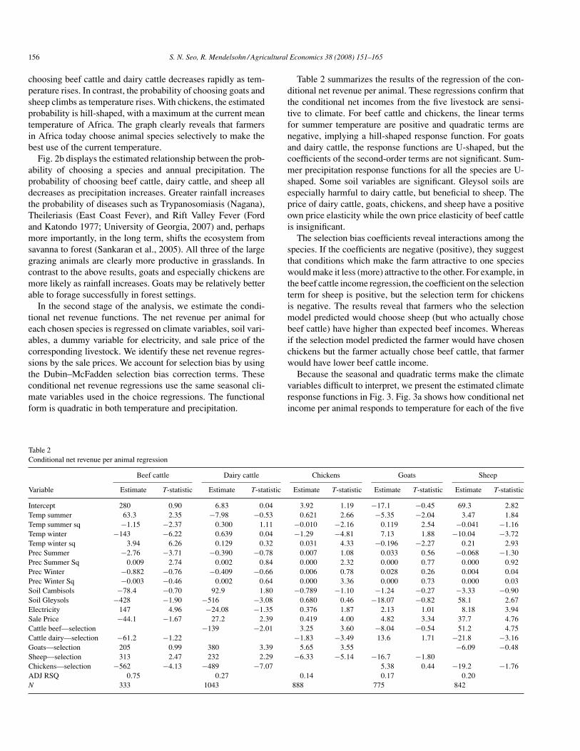
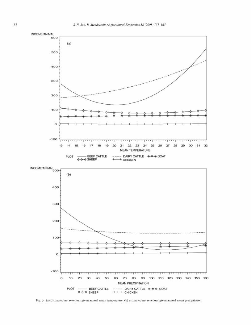
Because the seasonal and quadratic terms make the climatevariables difficult to interpret, we present the estimated climateresponse functions in Fig. 3. Fig. 3a shows how conditional netincome per animal responds to temperature for each of the five


Mean Temperature: C_Meat=19, C_Milk=19, Goat=24, Sheep=24, Chicken=21

P(Xi=1)

0.0

0.1

0.2

0.3

0.4

0.5

0.6

0.7

0.8

0.9

1.0

13 14 15 16 17 18 19 20 21 22 23 24 25 26 27 28 29 30 31 32

PLOT BEEF CATTLE DAIRY CATTLE

T_MAEAN_YR

SHEEP CHICKENGOAT

(a)

Mean Precipitation: C_Meat=58, C_Milk=63, Goat=68, Sheep=59, Chicken=76

P(Xi=1)

0.0

0.1

0.2

0.3

0.4

0.5

0.6

0.7

0.8

0.9

1.0

0 10 20 30 40 50 60 70 80 90 100 110 120 130 140 150 160

P_MANY_YR

PLOT BEEF CATTLE DAIRY CATTLESHEEP CHICKEN

GOAT

(b)

Fig. 2. (a) Estimated probability of selecting species given annual mean temperature; (b) estimated probability of selecting species given annual mean precipitation.


Fig. 3. (a) Estimated net revenues given annual mean temperature; (b) estimated net revenues given annual mean precipitation.


species. The conditional net income per animal is generallyhigher for beef cattle but it decreases rapidly as temperaturerises until the temperature reaches the African mean temper-ature, at which point farmers stop choosing beef cattle (seeFig. 2a). Commercial beef cattle are very profitable but theyare largely restricted to temperate zones in Africa. By con-trast, dairy cattle net revenue increases with higher tempera-ture. Dairy cattle operations are currently concentrated in thetemperate zones in East Africa and Southern Africa, but theyare more widely spread across the continent than beef cattle.The conditional net income per animal for goats, sheep, andchickens changes with temperature, but the magnitude of thechange is relatively small compared to cattle. Ceteris paribus,compared to beef cattle, these smaller animals—goats, sheep,and chickens—are likely to become relatively more attractiveto African farmers as temperatures rise. The figure also indi-cates that dairy cattle might substitute for beef cattle in highertemperatures.

Fig. 3b shows how conditional net revenue responds to pre-cipitation. It is important in interpreting these results to rec-ognize that increases in precipitation in Africa imply that landshifts from grassland to forest (not from unproductive to moreproductive pastureland). The conditional net revenue of beefcattle decreases precipitously the wetter it gets, whereas dairycattle net revenues remain quite stable over a large range of pre-cipitation. Sheep conditional net revenue also decreases withprecipitation. The conditional net revenues of goats and chick-ens increase slightly.

We also estimate a third set of regressions that predict thenumber of animals chosen of each species. We identify this thirdset of regressions by the percentage of grassland in each district.

Table 3Conditional number of animal regression

Beef cattle Dairy cattle Chickens Goats Sheep

Variable Estimate T-statistic Estimate T-statistic Estimate T-statistic Estimate T-statistic Estimate T-statistic

Intercept 223 0.82 −58.05 −3.20 1, 981 1.80 20.8 0.65 14.5 0.70Temp Summer −12.6 −0.52 3.78 2.90 −160 −2.08 2.35 1.28 7.59 4.31Temp Summer Sq 0.229 0.51 −0.063 −2.77 3.66 2.42 −0.037 −1.07 −0.123 −3.81Temp Winter −25.5 −1.09 1.21 0.83 0.046 0.00 −5.55 −1.96 −10.6 −4.34Temp Winter Sq 0.488 0.72 −0.055 −1.43 0.143 0.06 0.142 2.12 0.224 3.65Prec Summer 2.13 3.14 0.089 1.76 −2.42 −1.20 −0.042 −0.88 0.212 4.36Prec Summer Sq −0.01 −3.36 0.000 −1.89 0.022 2.85 0.000 0.71 0.000 −0.66Prec Winter −0.378 −0.39 0.204 3.10 1.96 0.80 0.010 0.13 0.148 1.69Prec Winter Sq −0.002 −0.29 −0.001 −2.45 −0.008 −0.49 0.000 −0.03 0.002 2.43Soil Cambisols 8.87 0.09 −4.31 −0.77 251 1.05 0.806 0.21 −2.33 −0.73Soil Gleysols 4.32 0.02 12.6 0.73 −436 −0.89 −26.8 −1.47 62.4 3.17Electricity dummy 145 5.35 0.665 0.36 298 3.59 6.04 3.51 −1.33 −0.71% grasslands 261 3.41 14.1 1.72 −208 −0.92 3.91 0.70 41.5 6.37Cattle beef—selection −4.73 −0.75 219 0.63 29.7 3.21 12.5 1.19Cattle dairy—selection 3.71 0.08 −132 −0.70 −5.34 −0.94 −35.2 −4.98Goats—selection −546 −3.14 −5.45 −0.48 497 0.89 17.9 1.59Sheep—selection 426 3.74 −16.5 −1.58 −325 −0.79 1.51 0.24Chickens—selection 86.1 0.72 23.3 3.44 −25.9 −2.53 16.6 1.67ADJ RSQ 0.33 0.12 0.12 0.03 0.09N 381 1036 876 774 810

Districts with more natural grassland can support more animals.As reported in Table 3, farms in districts with more grasslandchoose to own more beef cattle, dairy cattle, goats, and sheep perhousehold. Farms with electricity own more animals in generalbut fewer sheep. Soil variables are mostly insignificant, exceptfor the positive correlation between Gleysol soils and numberof sheep. Some of the selection bias correction terms are alsosignificant.

The number of each species of livestock is defined to be aquadratic function of summer and winter temperature and pre-cipitation as in the two previous regressions. For each animal,some of the climate variables are significant determinants of thenumber of that species. Summer temperature is significant fordairy cattle, chickens, and sheep, while winter temperature issignificant for goats and sheep. The number of goats and sheephas a U-shaped relationship with winter temperature. Summerprecipitation is significant for beef cattle, chickens, and sheep.The response is U shaped for chickens, but hill shaped for beefcattle and sheep.

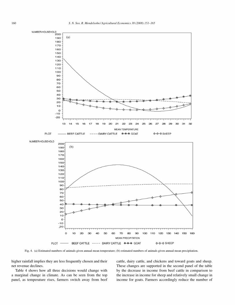
In Figs. 4a and b, we present how the estimated numbers oflivestock change in response to temperature and precipitation.Fig. 4a shows that the number of beef cattle decreases sharply astemperature increases while that of dairy cattle shows a slightdecrease. There are slight increases in the numbers of goatsand sheep. Chickens have a U-shaped response function withrespect to both temperature and precipitation, but we omit themfrom both figures because they are at an incompatible scale.Fig. 4b shows that the numbers of dairy cattle and goats arequite stable over a large range of precipitation, but the numberof beef cattle decreases rapidly with more rainfall. The sheepincrease in number as rainfall increases, despite the fact that


Fig. 4. (a) Estimated numbers of animals given annual mean temperature; (b) estimated numbers of animals given annual mean precipitation.

higher rainfall implies they are less frequently chosen and theirnet revenue declines.

Table 4 shows how all three decisions would change witha marginal change in climate. As can be seen from the toppanel, as temperature rises, farmers switch away from beef

cattle, dairy cattle, and chickens and toward goats and sheep.These changes are supported in the second panel of the tableby the decrease in income from beef cattle in comparison tothe increase in income for sheep and relatively small change inincome for goats. Farmers accordingly reduce the number of


Table 4Marginal effects of climate on outcomes

Beef cattle Dairy cattle Goats Sheep Chickens

Probability (%)Baseline 9.40% 27.3% 20.8% 21.8% 22.9%Temperature −1.29% −1.34% +1.09% +1.68% −0.84%Precipitation +0.2% −0.02% −0.01% −0.36% +0.22%

Net revenue ($/head)Baseline 221 145 11.5 17.8 1.55Temperature −5.57 +11.07 −0.42 +0.13 +0.07Precipitation −0.72 −0.01 +0.08 −0.02 +0.03

Number (head/farm)Baseline 57.4 5.65 11.3 13.07 137Temperature −7.99 +0.01 +1.24 +0.25 +11.1Precipitation −0.32 +0.02 −0.01 +0.21 +3.48

Note: Temperature is measured in ◦C and precipitation in mm/month.

beef cattle substantially as observed in the third panel while theyincrease the number of goats and sheep. As rainfall increases,farmers move away from beef cattle, dairy cattle, and sheeptoward goats and chickens. With the increase in rainfall, thenet income of beef cattle, dairy cattle, and sheep declines, butthe net income of goats and chickens increases. Although notcompletely consistent across the three analyses, the table clearlyindicates that farmers would substitute beef cattle for goats andsheep as temperature rises and they would substitute cattle andsheep for goats and chickens as rainfall increases.

5. Climate simulations

We now simulate the consequences of climate change usingthe parameter estimates from the previous section. We exam-ine a set of climate change scenarios predicted by AtmosphericOceanic General Circulation Models (AOGCMs). The climatescenarios reflect the A2 SRES scenarios from the followingthree models: the Canadian Climate Center (CCC) scenario(Boer et al., 2000), Center for Climate System Research (CCSR)(Emori et al., 1999), and Parallel Climate Model (PCM) (Wash-ington et al., 2003). The models were selected to provide a rangeof climate scenarios from mild (PCM) to severe (CCC). For eachmodel, we examine country-level climate change scenarios in2020, 2060, and 2100. For each climate scenario, we added

Table 5African average AOGCM climate scenarios

Current 2020 2060 2100

Temperature (◦C)CCC 23.3 +1.6 +3.6 +6.7CCSR 23.3 +2.0 +2.8 +4.1PCM 23.3 +0.6 +1.6 +2.5

Rainfall(mm/month)CCC 79.8 −3.7% −9.9% −18.4%CCSR 79.8 −7.0% −4.0% −22.0%PCM 79.8 +12.5% +1.1% +4.3%

the change in temperature predicted by each climate model tothe baseline temperature in each district. We also multiplied thepercentage change in precipitation predicted by each climatemodel by the baseline precipitation in each district or province.This gave us a new climate for every district in Africa for eachmodel and each time period.

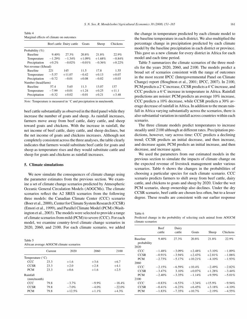
Table 5 summarizes the climate scenarios of the three mod-els for the years 2020, 2060, and 2100. The models predict abroad set of scenarios consistent with the range of outcomesin the most recent IPCC (Intergovernmental Panel on ClimateChange) report (Houghton et al., 2001; IPCC, 2007). In 2100,PCM predicts a 2◦C increase, CCSR predicts a 4◦C increase, andCCC predicts a 6◦C increase in temperature in Africa. Rainfallpredictions are noisier: PCM predicts an average 10% increase,CCC predicts a 10% decrease, while CCSR predicts a 30% av-erage decrease of rainfall in Africa. In addition to the mean rain-fall in Africa varying substantially across the scenarios, there isalso substantial variation in rainfall across countries within eachscenario.

The three climate models predict temperatures to increasesteadily until 2100 although at different rates. Precipitation pre-dictions, however, vary across time: CCC predicts a decliningtrend; CCSR predicts an initial decrease, and then increase,and decrease again; PCM predicts an initial increase, and thendecrease, and increase again.

We used the parameters from our estimated models in theprevious section to simulate the impacts of climate change onthe expected revenue of livestock management under variousscenarios. Table 6 shows the changes in the probabilities ofchoosing a particular species for each climate scenario. CCCscenario predicts farmers to shift away from beef cattle, dairycattle, and chickens to goats and sheep by 2020. Under the wetPCM scenario, sheep ownership also declines. Under the dryCCSR scenario, beef cattle are chosen less often, but to a lesserdegree. These results are consistent with our earlier response

Table 6Predicted change in the probability of selecting each animal from AOGCMclimate scenarios

Beef Dairycattle cattle Goats Sheep Chickens

Baseline 9.40% 27.3% 20.8% 21.8% 22.9%probability

2020CCC −1.48% −3.09% +2.48% +3.10% −1.89%CCSR −0.91% −3.94% +2.43% +2.81% −1.06%PCM −2.73% −5.17% +10.21% −4.10% −1.93%

2060CCC −2.15% −6.59% +10.4% −2.49% −2.82%CCSR −3.47% 3.10% +0.07% +1.28% −3.44%PCM −2.40% −3.35% −1.14% +9.59% −5.01%

2100CCC −0.83% −6.53% −3.34% +15.9% −9.94%CCSR −0.41% −6.23% +6.45% +3.18% −4.10%PCM −1.83% −7.35% +10.7% −2.19% −4.55%


Table 7Predicted change in net income per animal from AOGCM climate scenarios(US$/animal)


Baseline 224 150.1 11.1 16.7 1.602020

CCC +6.71 +19.9 −1.45 −1.06 +0.26CCSR −0.89 +19.9 −1.48 −1.12 +0.45PCM −82.7 +29.4 +3.75 −4.10 +3.02

2060CCC −78.8 +33.8 +2.37 −3.30 +3.08CCSR −44.6 +12.5 −1.92 −3.51 +0.84PCM +30.8 +32.8 −5.07 +0.17 +0.70

2100CCC +100.6 +68.1 −7.84 +1.69 +1.82CCSR −24.9 +49.8 +1.13 +0.75 +1.85PCM −66.8 +44.8 +1.90 −4.12 +3.46

Table 8Predicted change in numbers of each animal per farm from AOGCM climatescenarios (animals/farm)


Baseline 58.3 5.50 11.7 13.6 140.92020

CCC −12.9 +0.39 +3.94 +1.68 +41.8CCSR −9.91 +0.95 +4.13 +3.30 +8.86PCM −24.8 −0.46 +3.99 +31.1 +122.7

2060CCC −22.9 −0.34 +6.34 +29.8 +108CCSR −19.2 −1.07 +4.73 +7.13 +27.9PCM −19.8 −0.39 +12.4 +2.61 +60.7

2100CCC −27.6 −1.39 +24.8 +9.97 +204CCSR −37.2 +1.18 +8.54 +14.1 +207PCM −30.4 −0.59 +8.95 +34.1 +178

functions of species choices in Figs. 2a and b. This generaltrend also continues until 2100.

We show the changes in the conditional net incomes per ani-mal in Table 7. By 2100, the net income from beef cattle will

Table 9Predicted change in expected income from AOGCM climate scenarios (US$)

Mean (US$/farm) % Change Total (billions US$) Bootstrap lower 95% Bootstrap upper 95%

Expected income 882 602020

CCC −162 −18.4% −11.05 −220.1 −104CCSR −176 −19.9% −11.9 −236 −115PCM −137 −15.5% −9.33 −214 −60

2060CCC −101 −11.4% −6.88 −178 −23.9CCSR −220.1 −24.9% −14.9 −292 −148PCM +5.1 +0.58% +0.35 −70.8 +81.1

2100CCC +1488 +168% +101.2 +1343 +1633CCSR −71.3 −8.08% −4.85 −143 +0.59PCM 55.2 6.26% +3.76 −24.8 +135

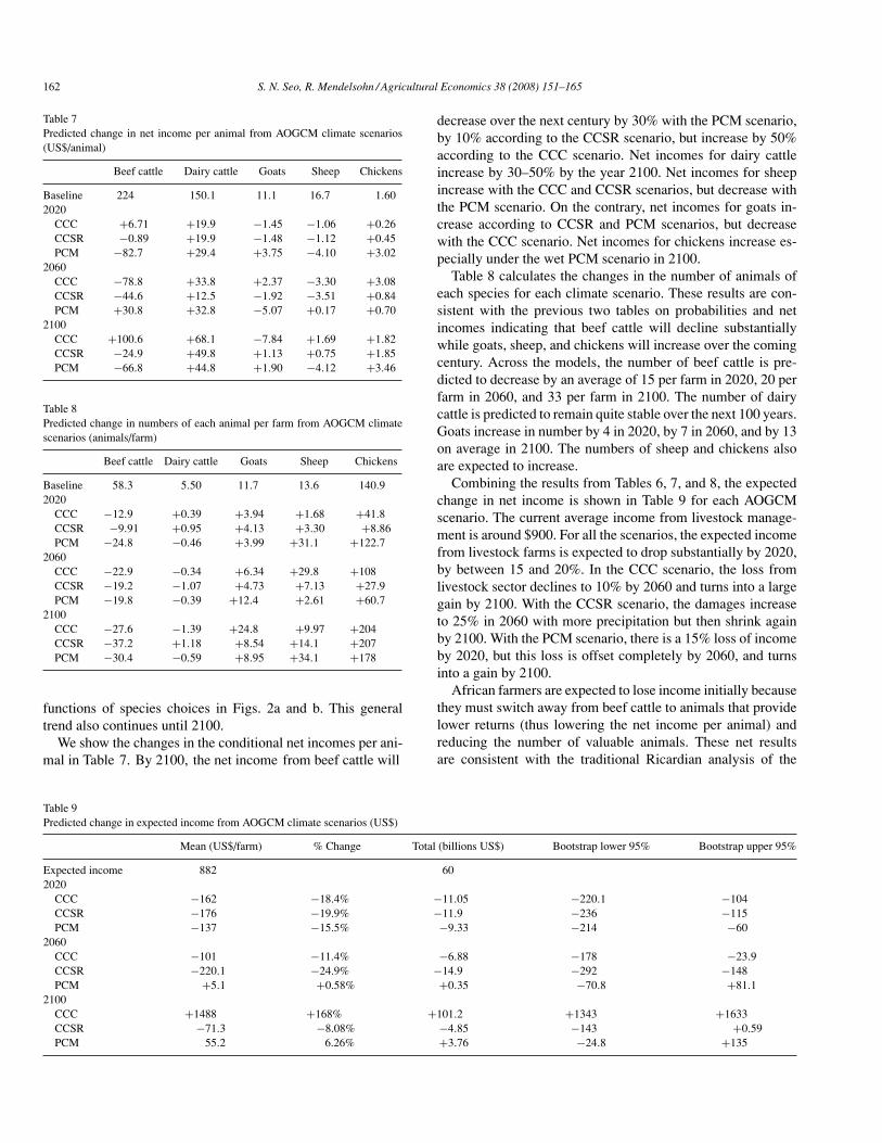
decrease over the next century by 30% with the PCM scenario,by 10% according to the CCSR scenario, but increase by 50%according to the CCC scenario. Net incomes for dairy cattleincrease by 30–50% by the year 2100. Net incomes for sheepincrease with the CCC and CCSR scenarios, but decrease withthe PCM scenario. On the contrary, net incomes for goats in-crease according to CCSR and PCM scenarios, but decreasewith the CCC scenario. Net incomes for chickens increase es-pecially under the wet PCM scenario in 2100.

Table 8 calculates the changes in the number of animals ofeach species for each climate scenario. These results are con-sistent with the previous two tables on probabilities and netincomes indicating that beef cattle will decline substantiallywhile goats, sheep, and chickens will increase over the comingcentury. Across the models, the number of beef cattle is pre-dicted to decrease by an average of 15 per farm in 2020, 20 perfarm in 2060, and 33 per farm in 2100. The number of dairycattle is predicted to remain quite stable over the next 100 years.Goats increase in number by 4 in 2020, by 7 in 2060, and by 13on average in 2100. The numbers of sheep and chickens alsoare expected to increase.

Combining the results from Tables 6, 7, and 8, the expectedchange in net income is shown in Table 9 for each AOGCMscenario. The current average income from livestock manage-ment is around $900. For all the scenarios, the expected incomefrom livestock farms is expected to drop substantially by 2020,by between 15 and 20%. In the CCC scenario, the loss fromlivestock sector declines to 10% by 2060 and turns into a largegain by 2100. With the CCSR scenario, the damages increaseto 25% in 2060 with more precipitation but then shrink againby 2100. With the PCM scenario, there is a 15% loss of incomeby 2020, but this loss is offset completely by 2060, and turnsinto a gain by 2100.

African farmers are expected to lose income initially becausethey must switch away from beef cattle to animals that providelower returns (thus lowering the net income per animal) andreducing the number of valuable animals. These net resultsare consistent with the traditional Ricardian analysis of the


same data (Seo et al., 2007). However, farmers will be ableto substitute species, reducing this initial damage over time.The 95% confidence interval was calculated for all of theseestimates using 200 bootstrap runs. The estimated damagesare significantly different from zero for most of the AOGCMscenarios in 2020, 2060, and 2100 except for the PCM scenariosin 2060 and 2100.

Table 9 also extends the analysis from the sample to all farmsin Africa. This leads to an estimate of the aggregate livestockimpact across Africa. The results suggest that the damage willvary from a loss of $9 to $12 billion in livestock income in2020, from zero to a $15 billion loss in 2060, and finally froma loss of $5 billion to a gain of $100 billion in 2100. In the longrun, climate change will be beneficial to the livestock sector inAfrica and this will offset some of the expected losses to crops(Kurukulasuriya et al., 2006).

6. Conclusion

This article uses a structural equation model to capture theendogenous choices made by farmers and their resulting ex-pected income. The model assumes that farmers choose theprofit-maximizing level of inputs for each animal, the speciesthat provides the highest net revenue, and the number of ani-mals of that species. The article tests whether these decisionsare influenced by climate. The resulting model gives insightsinto how farmers might adapt to climate change.

The model is applied to 5,000 livestock farmers in Africa.The multinomial choice model reveals that the probability ofselecting beef cattle, dairy cattle, and chickens diminish sharplyin warmer places. This is completely consistent with the obser-vation that commercial cattle operations are currently locatedonly in temperate locations across Africa, such as South Africaand Kenya. Furthermore, the model predicts that numbers ofgoats and sheep will increase with warming. This again is con-sistent with observations of where goats and sheep are currentlylocated, in relatively hot locations such as Burkina Faso, Niger,and Senegal. The model also reveals that beef cattle and sheepare more common in dryer areas, whereas goats and chickensare more common in wetter locations.

The conditional net revenue analysis supports the multino-mial choice results in general. Net revenue of beef cattle islower in warmer places, but net revenue of sheep is higherin warmer places. In a wetter place, net revenue from goatsand chickens is higher, but sheep net revenue is lower. Con-sequently, farmers move away from beef cattle to goats andsheep in warmer places. Farmers shift from cattle and sheepto goats and chickens in wetter places and the reverse in dryerplaces.

Finally, the predicted number of animals of each speciesis also consistent with the results from the multinomial logitchoice and conditional net revenue analysis. The number ofbeef cattle declines rapidly with warming while the number ofdairy cattle changes little. By contrast, the number of goats,

sheep, and chickens increases. With a precipitation increase(decrease), the number of beef cattle declines (increase) whilethe number of chickens increases (falls). As the net profitabilityof livestock falls, farmers will reduce their investments in thatlivestock and reduce their herds. This is especially evident withbeef cattle and warmer temperatures.

There has been very little quantitative research on animalhusbandry in Africa so there are few empirical studies withwhich to compare these results. A standard Ricardian analysiswas done by Seo et al. (2007), using the same data. The resultsof the standard Ricardian model are not exactly the same but areconsistent with the results in this article. That is, the Ricardiananalysis predicted that net revenues of large commercial farmswill fall with either rising temperature or rising rainfall levels,but those of small household farms will increase with warmingdue to their reliance on goats and sheep.

All the AOGCM predictions suggest that the expected profitfrom African livestock management will fall as early as 2020.Most of this effect is from the falling profitability of large beefcattle operations. Even small changes in temperature will besufficient to have a relatively large effect on beef cattle oper-ations. Additional warming will still be harmful, but farmerswill be able to make necessary substitutions to avoid furtherdamages, thereby lessening the magnitude of damage. Largefarms dependent on beef cattle will be especially hard hit. Incontrast, small farms that switch to sheep or goats may not be asvulnerable to higher temperatures compared with large farmsthat cannot make this switch.

Precipitation also plays an important role in the AOGCM re-sults. Scenarios with more precipitation, for example the CCSR2060 scenario, are more harmful. Because pastures and ecosys-tems in general are more productive with more rain, this resultmay seem counterintuitive. However, in Africa, increased pre-cipitation may increase animal diseases such as Nagana, EastCoast Fever, and Rift Valley Fever that are quite significantfor livestock (Ford and Katondo 1977; University of Geor-gia, 2007). Perhaps more importantly, more rain shifts savannaor grasslands into forest ecosystems (Sankaran et al., 2005).These grasslands are more productive for sheep, dairy cattle,and beef cattle. Reductions in precipitation from large to mod-erate levels appear to be beneficial to livestock. As long as thereis sufficient precipitation to support grasslands, livestock willgain.

This analysis reveals one way that farmers will be able toadapt to climate change. It suggests that small farmers willswitch species and move away from beef cattle, dairy cattle,and chickens toward goats and sheep. Small farmers will beable to make these changes without much change in expectedincome. However, climate change is predicted to reduce thenet incomes of large farms considerably. African policy mak-ers must be careful to encourage private adaptation during thisperiod of change. There may be nothing that can be done to sus-tain the large cattle operations that depend on current climate.Providing subsidies or other enticements for such operationsto continue once climate changes occur would only compound


the situation. Instead, governments should encourage farmersto change the composition of animals on their farms as needed.That is, they should inform farmers about how other livestockowners have coped with higher temperatures and share indige-nous knowledge. Governments should anticipate that farmerswill make changes on their lands and do whatever is needed tofacilitate these changes.

In interpreting these results, there are several caveats thatshould be kept in mind. First, this analysis does not include theeffect of global warming on prices. We assumed global mar-ket prices of livestock are relatively stable over the century. Ifinstead there are large changes in livestock prices, these resultswill overestimate the welfare effects of climate change. Second,we assumed adaptations can take place as needed. For exam-ple, farmers can switch across types of livestock as temperatureincreases and rainfall decreases. However, this may not be thecase if the adjustment requires a heavy capital investment orsubstantial learning. Third, we assumed that in forecasting cli-mate change impacts, the only thing that changes in the future isclimate. Many things, however, will change over the century, in-cluding population, technologies, institutional conditions, and

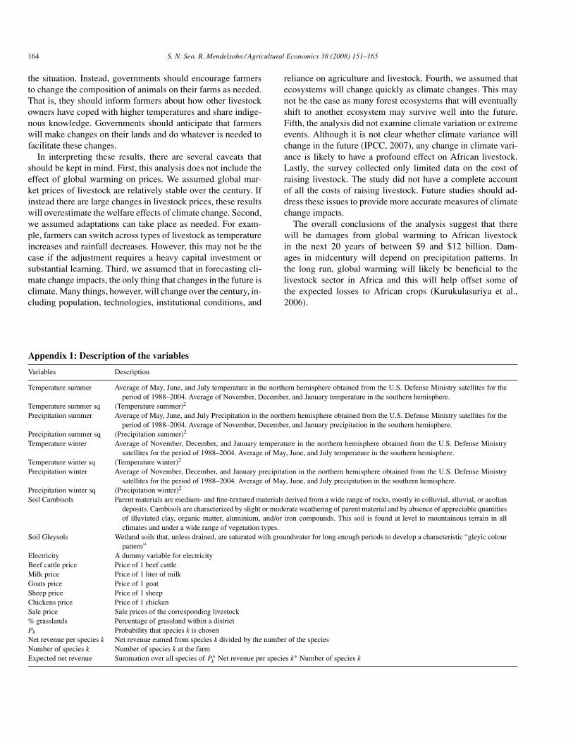
Appendix 1: Description of the variables

Variables Description

Temperature summer Average of May, June, and July temperature in the northern hemisphere obtained from the U.S. Defense Ministry satellites for theperiod of 1988–2004. Average of November, December, and January temperature in the southern hemisphere.

Temperature summer sq (Temperature summer)2

Precipitation summer Average of May, June, and July Precipitation in the northern hemisphere obtained from the U.S. Defense Ministry satellites for theperiod of 1988–2004. Average of November, December, and January precipitation in the southern hemisphere.

Precipitation summer sq (Precipitation summer)2

Temperature winter Average of November, December, and January temperature in the northern hemisphere obtained from the U.S. Defense Ministrysatellites for the period of 1988–2004. Average of May, June, and July temperature in the southern hemisphere.

Temperature winter sq (Temperature winter)2

Precipitation winter Average of November, December, and January precipitation in the northern hemisphere obtained from the U.S. Defense Ministrysatellites for the period of 1988–2004. Average of May, June, and July precipitation in the southern hemisphere.

Precipitation winter sq (Precipitation winter)2

Soil Cambisols Parent materials are medium- and fine-textured materials derived from a wide range of rocks, mostly in colluvial, alluvial, or aeoliandeposits. Cambisols are characterized by slight or moderate weathering of parent material and by absence of appreciable quantitiesof illuviated clay, organic matter, aluminium, and/or iron compounds. This soil is found at level to mountainous terrain in allclimates and under a wide range of vegetation types.

Soil Gleysols Wetland soils that, unless drained, are saturated with groundwater for long enough periods to develop a characteristic “gleyic colourpattern”

Electricity A dummy variable for electricityBeef cattle price Price of 1 beef cattleMilk price Price of 1 liter of milkGoats price Price of 1 goatSheep price Price of 1 sheepChickens price Price of 1 chickenSale price Sale prices of the corresponding livestock% grasslands Percentage of grassland within a districtPk Probability that species k is chosenNet revenue per species k Net revenue earned from species k divided by the number of the speciesNumber of species k Number of species k at the farmExpected net revenue Summation over all species of P ∗

k Net revenue per species k∗ Number of species k

reliance on agriculture and livestock. Fourth, we assumed thatecosystems will change quickly as climate changes. This maynot be the case as many forest ecosystems that will eventuallyshift to another ecosystem may survive well into the future.Fifth, the analysis did not examine climate variation or extremeevents. Although it is not clear whether climate variance willchange in the future (IPCC, 2007), any change in climate vari-ance is likely to have a profound effect on African livestock.Lastly, the survey collected only limited data on the cost ofraising livestock. The study did not have a complete accountof all the costs of raising livestock. Future studies should ad-dress these issues to provide more accurate measures of climatechange impacts.

The overall conclusions of the analysis suggest that therewill be damages from global warming to African livestockin the next 20 years of between $9 and $12 billion. Dam-ages in midcentury will depend on precipitation patterns. Inthe long run, global warming will likely be beneficial to thelivestock sector in Africa and this will help offset some ofthe expected losses to African crops (Kurukulasuriya et al.,2006).


References

Adams, R., McCarl, B., Segerson, K., Rosenzweig, C., Bryant, K. J., Dixon,B. L., Conner, R., Evenson, R. E., Ojima, D., 1999. The economic effectsof climate change on US agriculture. In: Mendelsohn, Neumann (Eds.),The Impact of Climate Change on the United States Economy. CambridgeUniversity Press, Cambridge, UK, pp. 18–54.

Andrews, D. K., Buchinsky, M., 2000. A three-step method for choosing thenumber of bootstrap repetitions. Econometrica 68, 23–51.

Boer, G., Flato, G., Ramsden, D., 2000. A transient climate change simulationwith greenhouse gas and aerosol forcing: projected climate for the 21stcentury. Clim. Dyn. 16, 427–450.

Bourguignon, F., Fournier, M., Gurgand, M., 2004. Selection bias correctionsbased on the multinomial logit model: Monte-Carlo comparisons. DELTA:Working Paper no. 20, DELTA.

Chow, G., 1983. Econometrics. McGraw-Hill Book Company, New York.De Janvry, A., Fafchamps, M., Sadoulet, E., 1991. Peasant household behavior

with missing markets: some paradoxes explained. Econ. J. 101(409), 1400–1417.

Dinar, A., Hassan, R., Mendelsohn, R., Benhin, J., 2008. Climate Changeand Agriculture in Africa: Impact Assessment and Adaptation Strategies.EarthScan, London.

Dubin, J. A., McFadden, D. L., 1984. An econometric analysis of residentialelectric appliance holdings and consumption. Econometrica 52(2), 345–362.

Emori, S. T. N., Abe-Ouchi, A., Namaguti, A., Kimoto, M., 1999. Coupledocean-atmospheric model experiments of future climate change with anexplicit representation of sulfate aerosol scattering. J. Meteorol. Soc. Jpn.77, 1299–1307.

Food and Agriculture Organization, 2004. The Digital Soil Map of the World(DSMW) CD-ROM, FAO, Rome, Italy.

Ford, J., Katondo, K., 1977. The Distribution of Tsetse flies in Africa. Organi-zation of African Unity, Nairobi, Kenya.

Greene, W. H., 1998. Econometric Analysis (3rd ed.). Prentice Hall, UpperSaddle River, NJ.

Heckman, J. J., 1979. Sample selection bias as a specification error. Economet-rica 47(1), 153–162.

Houghton, J. T., Ding, Y., Griggs, D. J., Noguer, M., van der Linden, P. J.,Xiaosu, D. (Eds.), 2001. Climate Change 2001: The Scientific Basis. Cam-bridge University Press, Cambridge, UK.

Intergovernmental Panel on Climate Change (IPCC), 2007. Summary for policymakers. In: Climate Change 2007: The Physical Science Basis. Contributionof Working Group I to the Fourth Assessment Report. Cambridge UniversityPress, Cambridge, UK.

Kurukulasuriya, P., Mendelsohn, R., Hassan, R., Benhin, J., Diop, M., Eid, H.M., Fosu, K. Y., Gbetibouo, G., Jain, S., Mahamadou, A., El-Marsafawy,S., Ouda, S., Ouedraogo, M., Sene, I., Maddision, D., Seo, S. N., Dinar, A.,2006. Will African agriculture survive climate change? World Bank Econ.Rev. 20(3), 367–388.

McCarthy, J., Canziani, O. F., Leary, N. A., Dokken, D. J., White, C. (Eds.),

2001. Climate Change 2001: Impacts, Adaptation, and Vulnerability. Cam-bridge University Press, Cambridge, UK.

McFadden, D. L., 1981. Econometric models of probabilistic choice. In: Mc-Fadden, D. (Ed.). Structural Analysis of Discrete Data and EconometricApplications. MIT Press, Cambridge, MA, pp. 198–272.

McFadden, D. L., 1999. Chapter 1. Discrete response models. University ofCalifornia at Berkeley, Lecture Note.

Mendelsohn, R., Nordhaus, W. D., Shaw, D., 1994. The impact of globalwarming on agriculture: a Ricardian analysis. Am. Econ. Rev. 84, 753–771.

Mendelsohn, R., Kurukulasuriya, P., Basist, A., Kogan, F., Williams, C., 2007.Measuring climate change impacts with satellite versus weather station data.Clim. Change 81, 71–83.

Moll, H. A. J., 2005. Costs and benefits of livestock systems and the role ofmarket and nonmarket relationships. Agric. Econ. 32, 181–193.

Oklahoma State University, 2007. Breeds of Livestock. Available athttp://www.ansi.okstate.edu/breeds

Pearce, D. W., Achanta, A. N., Cline, W. R., Fankhauser, S., Pachauri, R., Tol,R. S. J., Vellinga, P., 1996. The social costs of climate change: greenhousedamage and benefits of control. In: Bruce, J., Lee, H., Haites, E. (Eds.).Climate Change 1995: Economic and Social Dimensions of Climate Change.Cambridge University Press, Cambridge, UK.

Sankaran, M., Hanan, N., Scholes, R., Ratnam, J., Augustine, D., Cade, B.,Gignoux, J., Higgins, S., Le Roux, X., Ludwig, F., Ardo, J., Banyikwa, F.,Bronn, A., Bucini, G., Caylor, K., Coughenour, M., Diouf, A., Ekaya, W.,Feral, C., February, E., Frost, P., Hiernaux, P., Hrabar, H., Metzger, K.,Prins, H., Ringrose, S., Sea1, W., Tews, J., Worden, J., Zambatis, N., 2005.Determinants of woody cover in African savannas. Nature 438, 846–849.

Seo, S. N., Mendelsohn, R., Kurukulasuriya, P., 2007. Climate change impactson animal husbandry in Africa: a Ricardian analysis. World Bank PolicyResearch Working Paper 4261, Washington, DC.

Seo, S. N., Mendelsohn, R., 2007. Climate change adaptation in Africa: amicroeconomic analysis of livestock choice. World Bank Policy ResearchWorking Paper 4277, Washington, DC.

Singh, I., Squire, L., Strauss, J., 1986. A survey of agricultural householdmodels: recent findings and policy implications. World Bank Econ. Rev.1(1), 149–179.

Tol, R. S. J., 2002. New estimates of the damage costs of climate change, partI: benchmark estimates. Environ. Resour. Econ. 21(1), 47–73.

Train, K., 2003. Discrete Choice Methods with Simulation. Cambridge Univer-sity Press, Cambridge, UK.

United States Department of Agriculture (USDA), 2002. Censusof Agriculture, Available at http://www.nass.usda.gov/census/census02/volume1/us/st99_1_002_002.pdf

University of Georgia, College of Veterinary Medicine, 2007. For-eign Animal Diseases: The Greybook, Available at http://www.vet.uga.edu/vpp/grey_book02

Washington, W., Weatherly, J., Meehl, G., Semtner, A., Bettge, T., Craig, A.,Strand, W., Arblaster, J., Wayland, V., James, R., Zhang, Y., 2003. Parallelclimate model (PCM): control and transient scenarios. Clim. Dyn. 16, 755–774.

Documents

Measuring impacts and adaptations to climate change: a ...huardda/articles/seo08.pdf · AGRICULTURAL ECONOMICS Agricultural Economics 38 (2008) 151–165 Measuring impacts and adaptations