Embed Size (px)
Citation preview
A&A 585, A68 (2016)DOI: 10.1051/0004-6361/201526485c© ESO 2015
Astronomy&
Astrophysics
Measuring dark energy with the Eiso – Ep correlationof gamma-ray bursts using model-independent methods
J. S. Wang1, F. Y. Wang1,2,3, K. S. Cheng2, and Z. G. Dai1,3
1 School of Astronomy and Space Science, Nanjing University, 210093 Nanjing, PR Chinae-mail: [email protected]
2 Department of Physics, University of Hong Kong, Pokfulam Road, Hong Kong, PR China3 Key Laboratory of Modern Astronomy and Astrophysics (Nanjing University), Ministry of Education, 210093 Nanjing, PR China
Received 7 May 2015 / Accepted 28 September 2015
ABSTRACT
We use two model-independent methods to standardize long gamma-ray bursts (GRBs) using the Eiso − Ep correlation (log Eiso =a + b log Ep), where Eiso is the isotropic-equivalent gamma-ray energy and Ep is the spectral peak energy. We update 42 long GRBsand attempt to constrain the cosmological parameters. The full sample contains 151 long GRBs with redshifts from 0.0331 to 8.2. Thefirst method is the simultaneous fitting method. We take the extrinsic scatter σext into account and assign it to the parameter Eiso . Thebest-fitting values are a = 49.15± 0.26, b = 1.42± 0.11, σext = 0.34± 0.03 and Ωm = 0.79 in the flat ΛCDM model. The constraint onΩm is 0.55 < Ωm < 1 at the 1σ confidence level. If reduced χ2 method is used, the best-fit results are a = 48.96±0.18, b = 1.52±0.08,and Ωm = 0.50 ± 0.12. The second method uses type Ia supernovae (SNe Ia) to calibrate the Eiso − Ep correlation. We calibrate 90high-redshift GRBs in the redshift range from 1.44 to 8.1. The cosmological constraints from these 90 GRBs are Ωm = 0.23+0.06
−0.04 forflat ΛCDM and Ωm = 0.18 ± 0.11 and ΩΛ = 0.46 ± 0.51 for non-flat ΛCDM. For the combination of GRB and SNe Ia sample, weobtain Ωm = 0.271± 0.019 and h = 0.701± 0.002 for the flat ΛCDM and the non-flat ΛCDM, and the results are Ωm = 0.225± 0.044,ΩΛ = 0.640 ± 0.082, and h = 0.698 ± 0.004. These results from calibrated GRBs are consistent with that of SNe Ia. Meanwhile,the combined data can improve cosmological constraints significantly, compared to SNe Ia alone. Our results show that the Eiso − Ep
correlation is promising to probe the high-redshift Universe.
Key words. cosmological parameters – dark energy – gamma rays: general
1. Introduction
Gamma-ray bursts (GRBs) are the most violent explosions inthe Universe, with the highest isotropic energy up to 1054 erg(for reviews, see Mészáros 2006; Zhang 2007; Gehrels et al.2009). Thus, they can be detected to the edge of the visibleUniverse (Ciardi & Loeb 2000; Lamb & Reichart 2000; Wanget al. 2012). For instance, the spectroscopically confirmed red-shift of GRB090423 is about 8.2 (Tanvir et al. 2009; Salvaterraet al. 2009). Therefore, they are promising probes for the high-redshift Universe (for a recent review, see Wang et al. 2015).Many studies have been carried out to use GRBs for cosmologi-cal purposes, such as the star formation rate (Totani 1997; Wijerset al. 1998; Porciani & Madau 2001; Wang & Dai 2009, 2011a),the intergalactic medium metal enrichment (Barkana & Loeb2004; Wang et al. 2012), dark energy (Dai et al. 2004; Friedman& Bloom 2005; Schaefer 2007; Basilakos & Perivolaropoulos2008; Wang et al. 2011b), reionization (Totani et al. 2006;Gallerani et al. 2008; Wang 2013), possible anisotropic acceler-ation (Wang & Wang 2014a), and the two-point correlation (Li& Lin 2015).
To constrain the cosmological parameters, standard rulersor candles such as baryon acoustic oscillations (BAO; Coleet al. 2005; Eisenstein et al. 2005; Anderson et al. 2014), cos-mic microwave background (CMB; Komatsu et al. 2011; PlanckCollaboration XVI 2013; Planck Collaboration XIII 2015) and
SNe Ia (Riess et al. 1998; Perlmutter et al. 1999; Suzuki et al.2012) are required. The redshifts of BAO and SNe Ia are low,however, and the CMB is only a snapshot of cosmic expansion.Some parameters, such as the density and EOS parameter of darkenergy (Wang 2012; Wang & Dai 2014; Wang & Wang 2014b),might evolve with redshift. GRBs can probe the evolution ofthese parameters at high redshifts and serve as complementarytools for SNe Ia. The study of these evolutions can differenti-ate dark energy models. Some luminosity correlations have beenproposed to standardize GRBs (Amati et al. 2002; Ghirlandaet al. 2004a; Liang & Zhang 2005). Ghirlanda et al. (2004a)found a tight correlation between collimated energy Eγ and thepeak energy Ep of νFν spectrum. Dai et al. (2004) used this cor-relation to constrain cosmological parameters with 12 GRBs.Liang & Zhang (2005) found the Eiso − Ep − tb correlationand used this correlation to constrain cosmological parameters.Recently, Wang et al. (2011b) constrained cosmological param-eters with 109 GRBs using six GRB empirical correlations, andfound Ωm = 0.31+0.13
−0.10 in the flat Λ cold dark matter (CDM)model. Other attempts have also been made to standardize GRBs(Ghirlanda et al. 2004b; Friedman & Bloom 2005; Schaefer2007; Wang et al. 2007; Liang et al. 2008; Kodama et al. 2008;Qi et al. 2009; Cardone et al. 2010; Wang & Dai 2011c). Thesemethods of standardizing the long GRBs are mainly based onsome empirical correlations, such as the Eiso − Ep (Amati et al.2002), Ep − Lp (Schaefer 2003; Wei & Gao 2003), and Ep − Eγ
Article published by EDP Sciences A68, page 1 of 9
A&A 585, A68 (2016)
(Ghirlanda et al. 2004a), where Lp is the peak luminosity, Ep isthe peak energy in cosmological rest frame, Eiso is the isotropic-equivalent energy, and Eγ is the collimation-corrected energy.Correlations within X-ray afterglow light curves have also beenstudied (Dainotti et al. 2008, 2010; Qi & Lu 2010).
In this paper, we focus on the usage of the Eiso − Ep correla-tion. Amati et al. (2002) discovered this correlation with a smallsample of BeppoSAX GRBs. Since many more GRBs are de-tected, attempts have been made to use this correlation for thepurpose of cosmology. Amati et al. (2008) used a simultaneousfitting method to constrain the Eiso − Ep correlation coefficientsand cosmological parameters together with 70 long GRBs. Theextrinsic scatter σext was taken into consideration in this method(D’Agostini 2005). Amati et al. (2008) assigned σext to Ep andfound 0.04 < Ωm < 0.40 and σext = 0.17 ± 0.02 at 1σ con-fidence level in the flat ΛCDM Universe. For non-flat ΛCDMmodel, the results are Ωm ∈ [0.04, 0.40] and ΩΛ < 1.05 (Amatiet al. 2008). However, Ghirlanda (2009) doubted this result. Heclaimed that the extrinsic scatter term should be assigned to Eiso.This is consistent with D’Agostini (2005), who described thatthe extrinsic scatter σext should be assigned to the parameter thatalso depends on hidden variables (cosmological parameters inour study). We discuss this point in detail in Sect. 3.1. However,this would lead to no constraint on cosmological parameters withthe same 70 GRBs from Amati et al. (2008). We test it again witha larger sample in this paper.
The calibration method is also helpful to standardize GRBs.Imitating the example of standardizing the standard candleof SNe Ia with Cepheid variables, GRBs can also be cali-brated with SNe Ia (Liang et al. 2008; Kodama et al. 2008;Wei 2010; Lin et al. 2016). This method is also cosmologi-cal model independent. Liang et al. (2008) calibrated 42 highredshift GRBs with SNe Ia. Five interpolation methods wereused and the results were consistent with each other. Wei (2010)standardized 59 high-redshift GRBs with SNe Ia, using theEiso − Ep correlation, and found that GRBs can improve theconstraint on cosmological parameters. Wang & Dai (2011c)calibrated 116 GRBs with Union 2 SNe Ia with cosmographicparameters.
We use 151 GRBs, 109 of which are taken from Amatiet al. (2008) and Amati et al. (2009). The remaining 42 GRBsare the updated long GRBs, which were detected by FermiGBM, Konus-Wind, Swift-BAT, and Suzaku-WAM. The energyband, fluence, low (α), high (β) energy photon indices, spec-tral peak energy, and redshift are taken from the refined anal-ysis of the corresponding GRB team. We test whether this largerGRB sample can help to constrain cosmological models better.First, we constrain the cosmological parameters and coefficientsof the Eiso − Ep correlation simultaneously. Then, we calibratethese GRBs with SNe Ia using the Eiso − Ep correlation. At last,we compare these two methods and discuss them.
This paper is organized as follows. In the next section, we in-troduce the GRBs data and perform the K-correction. In Sect. 3,we test whether the redshift evolution of the Eiso−Ep correlationis significant, and use a simultaneous fitting method to constraincosmological parameters and coefficients of the Eiso − Ep corre-lation. In Sect. 4, we use SNe Ia to calibrate the Eiso−Ep correla-tion, then we use these calibrated GRBs to constrain cosmologi-cal parameters. Summary and discussions are given in Sect. 5.
2. Updated GRB sample
We collect all GRBs with information of redshift, flu-ence, peak energy, and photon indices from GCN Circulars
Archive1 Cucchiara et al. (2011) and Gendre et al. (2013) un-til February 13, 2014. The updated sample contains 42 updatedlong GRBs. We list these GRBs in Table 1. The spectra of theseGRBs are obtained from the refined analysis of Fermi GBMteam, Konus-Wind team, Swift-BAT team, and Suzaku-WAMteam. The redshifts extend from 0.34 to 5.91. The spectrum ismodeled by a broken power law (Band et al. 1993),
Φ(E) =
⎧⎪⎪⎪⎨⎪⎪⎪⎩AEαe−(2+α)E/Ep,obs if E ≤ α−β2+αEp,obs
BEβ otherwise,(1)
where Ep,obs is the observed peak energy, α and β are the lowand high energy photon indices, respectively. We take the typicalspectral index values for those GRB whose indices are not givenout in the references, i.e., α = −1.0 and β = −2.2 (Salvaterraet al. 2009).
With these spectra parameters, we can obtain the peak energyin the cosmological rest frame by Ep = Ep,obs × (1 + z) and thebolometric fluence in the band of 1 − 104 keV by (Bloom et al.2001)
S bolo = S ×∫ 104/(1+z)
1/(1+z)EΦ(E)dE∫ Emax
EminEΦ(E)dE
, (2)
where S is the observed fluence, Emin and Emax are the detectionlimits of the instrument, and z is the redshift.
In the Eiso − Ep plane, Ep is an observed value, which is notdependent on the cosmological model. However, Eiso dependson the cosmological model from
Eiso = 4πd2LS bolo(1 + z)−1, (3)
where dL is the luminosity distance. Assuming a flat ΛCDMmodel, the dL can be expressed with Hubble expansion rate
dL(Ωm, z) = (1 + z)c
H0
∫ z
0
dz′√Ωm(1 + z)3 + 1 −Ωm
, (4)
where Ωm is the matter density at present, and H0 is the Hubbleconstant. Since the Hubble constant is precisely measured, wetake H0 = 67.8 km s−1 Mpc−1 (Planck Collaboration XVI 2013;Planck Collaboration XIII 2015), except when we use the combi-nation data of SNe and GRB to constrain cosmological models.
We list 42 updated GRBs in Table 1. The isotropic en-ergy Eiso is calculated with benchmark parameters with Ωm =0.308 for the flat ΛCDM Universe (Planck Collaboration XVI2013; Planck Collaboration XIII 2015). During the calculation,we only take the errors propagating from the spectrum parame-ters, namely observed fluence S and peak energy Ep,obs. The un-certainties from other parameters are attributed into the extrinsicscatter σext.
3. The Eiso – Ep correlation and constraintson cosmological parameters
3.1. The Eiso – Ep correlation
To constrain cosmological models more precisely, we combineour updated 42 GRBs with 109 GRBs from Amati et al. (2008)and Amati et al. (2009). The full sample contains 151 GRBs and
1 http://gcn.gsfc.nasa.gov/gcn3_archive.html
A68, page 2 of 9
J. S. Wang et al.: Measuring dark energy with Eiso − Ep correlation
Table 1. 42 updated long GRBs.
GRB Redshift S bolo(10−5 erg cm−2) Ep(keV) Eisoa (1053 erg) Instrumentsb Refs. for spectrum
100413 3.90 2.36 ± 0.77 1783.60 ± 374.85 7.31 ± 4.56 SW (1)100621 0.54 5.75 ± 0.64 146.49 ± 23.90 0.46 ± 0.20 KW (2)100704 3.60 0.70 ± 0.07 809.60 ± 135.70 1.91 ± 0.61 KW (3)100728B 2.45 0.29 ± 0.01 359.11 ± 48.34 0.42 ± 0.12 FG (4)100814 1.44 1.39 ± 0.23 312.32 ± 48.80 0.77 ± 0.31 KW (5)100906 1.73 3.56 ± 0.55 387.23 ± 244.07 2.77 ± 1.18 KW (6)110205 2.22 3.32 ± 0.68 740.60 ± 322.00 4.04 ± 1.82 KW/SB/SW (7)110213 1.46 1.55 ± 0.23 223.86 ± 70.11 0.88 ± 0.41 KW (8)110422 1.77 9.32 ± 0.02 421.04 ± 13.85 7.58 ± 1.67 KW (9)110503 1.61 2.76 ± 0.21 572.25 ± 50.95 1.89 ± 0.55 KW (10)110715 0.82 2.73 ± 0.24 218.40 ± 20.93 0.51 ± 0.16 KW (11)110731 2.83 2.51 ± 0.01 1164.32 ± 49.79 4.62 ± 1.06 KW (12)110818 3.36 1.05 ± 0.08 1117.47 ± 241.11 2.56 ± 0.85 FG (13)111008 5.00 1.06 ± 0.11 894.00 ± 240.00 4.82 ± 1.61 KW (14)111107 2.89 0.18 ± 0.03 420.44 ± 124.58 0.34 ± 0.14 FG (15)111209 0.68 69.47 ± 8.72 519.87 ± 88.88 8.77 ± 3.61 KW (16)120119 1.73 4.62 ± 0.59 417.38 ± 54.56 3.60 ± 1.17 KW (17)120326 1.80 0.44 ± 0.02 129.97 ± 10.27 0.37 ± 0.11 FG (18)120724 1.48 0.15 ± 0.02 68.45 ± 18.60 0.09 ± 0.05 SB (19)120802 3.80 0.43 ± 0.07 274.33 ± 93.04 1.28 ± 0.78 SB (20)120811C 2.67 0.74 ± 0.07 157.49 ± 20.92 1.24 ± 0.74 SB (21)120909 3.93 2.69 ± 0.23 1651.55 ± 123.25 8.44 ± 2.72 KW (22)120922 3.10 1.59 ± 0.18 156.62 ± 0.04 3.41 ± 2.12 SB (23)121128 2.20 0.87 ± 0.07 243.20 ± 12.80 1.04 ± 0.35 KW (24)130215 0.60 4.84 ± 0.12 247.54 ± 100.61 0.47 ± 0.24 FG (25)130408 3.76 0.99 ± 0.17 1003.94 ± 137.98 2.89 ± 0.96 KW (26)130420A 1.30 1.73 ± 0.06 128.63 ± 6.89 0.79 ± 0.22 FG (27)130427A 0.34 311.17 ± 0.47 1112.20 ± 6.70 9.51 ± 3.01 FG (28)130505 2.27 4.56 ± 0.09 2063.37 ± 101.37 5.77 ± 1.79 KW (29)130514 3.60 1.88 ± 0.25 496.80 ± 151.80 5.13 ± 2.05 KW/SB (30)130518 2.49 12.34 ± 0.08 1382.04 ± 31.41 18.31 ± 4.97 FG (31)130606 5.91 0.49 ± 0.09 2031.54 ± 483.70 2.86 ± 1.16 KW (32)130610 2.09 0.82 ± 0.05 911.83 ± 132.65 0.90 ± 0.30 FG (33)130612 2.01 0.08 ± 0.01 186.07 ± 31.56 0.08 ± 0.03 FG (34)130701A 1.16 0.46 ± 0.04 191.80 ± 8.62 0.17 ± 0.05 KW (35)130831A 0.48 1.29 ± 0.07 81.35 ± 5.92 0.08 ± 0.03 KW (36)130907A 1.24 75.21 ± 4.76 881.77 ± 24.62 31.40 ± 7.97 KW (37)131030A 1.29 1.05 ± 0.10 405.86 ± 22.93 0.48 ± 0.15 KW (38)131105A 1.69 4.75 ± 0.16 547.68 ± 83.53 3.54 ± 1.28 FG (39)131117A 4.04 0.05 ± 0.01 221.85 ± 37.31 0.16 ± 0.09 SB (40)140206A 2.73 1.69 ± 0.03 447.60 ± 22.38 2.93 ± 0.74 FG (41)140213A 1.21 2.53 ± 0.04 176.61 ± 4.42 1.01 ± 0.26 FG (42)
Notes. (a) Eiso is computed with benchmark parameters: H0 = 67.8 km s−1 Mpc−1 and Ωm = 0.308; (b) Instruments: FG = Fermi GBM,KW = Konus-Wind, SB = Swift-BAT and SW = Suzaku-WAM.
References. for the spectrum parameters: (1) Sugita et al. (2010); (2) Golenetskii et al. (2010a); (3) Golenetskii et al. (2010b); (4) von Kienlin(2010); (5) Golenetskii et al. (2010c); (6) Golenetskii et al. (2010d); (7) Cucchiara et al. (2011); (8) Golenetskii et al. (2011a); (9) Golenetskiiet al. (2011b); (10) Golenetskii et al. (2011c); (11) Golenetskii (2011d); (12) Golenetskii et al. (2011e); (13) Xiong (2011); (14) Golenetskii et al.(2011f); (15) Pelassa (2011); (16) Golenetskii et al. (2012c); (17) Golenetskii et al. (2012a); (18) Collazzi (2012); (19) Krimm et al. (2012a);(20) Stamatikos et al. (2012); (21) Krimm et al. (2012b); (22) Golenetskii et al. (2012b); (23) Krimm et al. (2012c); (24) Golenetskii et al.(2013a) (25) Younes & Bhat (2013); (26) Golenetskii et al. (2013b); (27) Xiong & Rau (2013); (28) von Kienlin (2013); (29) Golenetskii et al.(2013c); (30) Palshin et al. (2013); (31) Xiong (2013); (32) Golenetskii et al. (2013d) (33) Fitzpatrick & Pelassa (2013); (34) Fitzpatrick (2013);(35) Golenetskii et al. (2013e); (36) Golenetskii et al. (2013f) (37) Golenetskii et al. (2013g); (38) Golenetskii et al. (2013h); (39) Fitzpatrick &Jenke (2013); (40) Krimm et al. (2013); (41) von Kienlin & Bhat (2014); (42) Zhang et al. (2014).
covers the redshift range from 0.0331 to 8.2. We parameterizethe Eiso − Ep correlation as follows:
logEiso
erg= a + b log
Ep
keV, (5)
where a and b are the intercept and slope. Here Ep has beencorrected into the cosmological rest frame.
Before constraining cosmological models, we test the pos-sible redshift evolution of the Eiso − Ep correlation using themaximum likelihood method. The full data is divided into fourredshift bins: [0.0331, 0.958], [0.966, 1.613], [1.619, 2.671],and [2.69, 8.2]. Each bin almost includes the same number ofGRBs. The results are shown in Table 2. We give out the best-fitvalues and 1σ uncertainties in the coefficients a, b, and the ex-trinsic scatter σext. The σext is almost constant in different bins.
A68, page 3 of 9
A&A 585, A68 (2016)
Table 2. Eiso − Ep correlation fitting results of full data and four redshift bins.
Redshift range a b σext GRB numberFull data 49.21 ± 0.24 1.48 ± 0.09 0.34 ± 0.04 151[0.0331, 0.958] 48.92 ± 0.36 1.58 ± 0.15 0.34 ± 0.07 37[0.966, 1.613] 49.54 ± 0.61 1.37 ± 0.23 0.40 ± 0.07 38[1.619, 2.671] 49.62 ± 0.64 1.33 ± 0.24 0.33 ± 0.07 38[2.69, 8.1] 49.62 ± 0.60 1.34 ± 0.22 0.25 ± 0.07 38
Notes. The best-fit value, 1σ uncertainties, and extrinsic scatter σext are given.
0.0 0.5 1.0 1.5 2.0 2.5 3.0 3.5
49
50
51
52
53
54
55
Log�Ep�keV�
Log�E
iso�
erg�
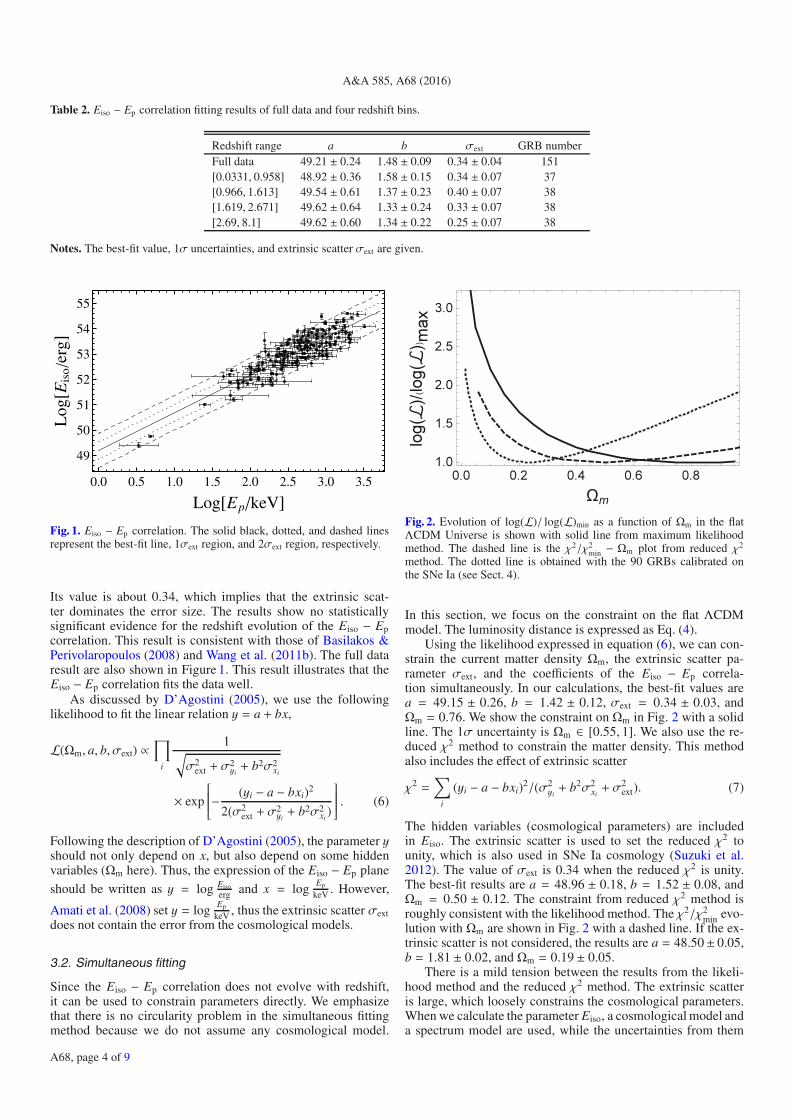
Fig. 1. Eiso − Ep correlation. The solid black, dotted, and dashed linesrepresent the best-fit line, 1σext region, and 2σext region, respectively.
Its value is about 0.34, which implies that the extrinsic scat-ter dominates the error size. The results show no statisticallysignificant evidence for the redshift evolution of the Eiso − Epcorrelation. This result is consistent with those of Basilakos &Perivolaropoulos (2008) and Wang et al. (2011b). The full dataresult are also shown in Figure 1. This result illustrates that theEiso − Ep correlation fits the data well.
As discussed by D’Agostini (2005), we use the followinglikelihood to fit the linear relation y = a + bx,
L(Ωm, a, b, σext) ∝∏
i
1√σ2
ext + σ2yi+ b2σ2
xi
× exp
⎡⎢⎢⎢⎢⎢⎣− (yi − a − bxi)2
2(σ2ext + σ
2yi+ b2σ2
xi)
⎤⎥⎥⎥⎥⎥⎦ . (6)
Following the description of D’Agostini (2005), the parameter yshould not only depend on x, but also depend on some hiddenvariables (Ωm here). Thus, the expression of the Eiso − Ep plane
should be written as y = log Eisoerg and x = log Ep
keV . However,
Amati et al. (2008) set y = log Ep
keV , thus the extrinsic scatter σextdoes not contain the error from the cosmological models.
3.2. Simultaneous fitting
Since the Eiso − Ep correlation does not evolve with redshift,it can be used to constrain parameters directly. We emphasizethat there is no circularity problem in the simultaneous fittingmethod because we do not assume any cosmological model.
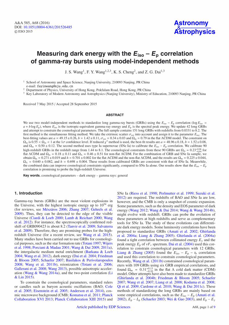
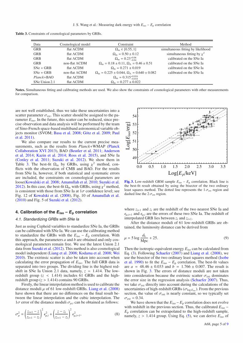
Fig. 2. Evolution of log(L)/ log(L)min as a function of Ωm in the flatΛCDM Universe is shown with solid line from maximum likelihoodmethod. The dashed line is the χ2/χ2
min − Ωm plot from reduced χ2
method. The dotted line is obtained with the 90 GRBs calibrated onthe SNe Ia (see Sect. 4).
In this section, we focus on the constraint on the flat ΛCDMmodel. The luminosity distance is expressed as Eq. (4).
Using the likelihood expressed in equation (6), we can con-strain the current matter density Ωm, the extrinsic scatter pa-rameter σext, and the coefficients of the Eiso − Ep correla-tion simultaneously. In our calculations, the best-fit values area = 49.15 ± 0.26, b = 1.42 ± 0.12, σext = 0.34 ± 0.03, andΩm = 0.76. We show the constraint on Ωm in Fig. 2 with a solidline. The 1σ uncertainty is Ωm ∈ [0.55, 1]. We also use the re-duced χ2 method to constrain the matter density. This methodalso includes the effect of extrinsic scatter
χ2 =∑
i
(yi − a − bxi)2/(σ2yi+ b2σ2
xi+ σ2
ext). (7)
The hidden variables (cosmological parameters) are includedin Eiso. The extrinsic scatter is used to set the reduced χ2 tounity, which is also used in SNe Ia cosmology (Suzuki et al.2012). The value of σext is 0.34 when the reduced χ2 is unity.The best-fit results are a = 48.96 ± 0.18, b = 1.52 ± 0.08, andΩm = 0.50 ± 0.12. The constraint from reduced χ2 method isroughly consistent with the likelihood method. The χ2/χ2
min evo-lution with Ωm are shown in Fig. 2 with a dashed line. If the ex-trinsic scatter is not considered, the results are a = 48.50± 0.05,b = 1.81 ± 0.02, and Ωm = 0.19 ± 0.05.
There is a mild tension between the results from the likeli-hood method and the reduced χ2 method. The extrinsic scatteris large, which loosely constrains the cosmological parameters.When we calculate the parameter Eiso, a cosmological model anda spectrum model are used, while the uncertainties from them
A68, page 4 of 9
J. S. Wang et al.: Measuring dark energy with Eiso − Ep correlation
Table 3. Constraints of cosmological parameters by GRBs.
Data Cosmological model Constraint MethodGRB flat ΛCDM Ωm ∈ [0.55, 1] simultaneous fitting by likelihoodGRB flat ΛCDM Ωm = 0.50 ± 0.12 simultaneous fitting by χ2
GRB flat ΛCDM Ωm = 0.23+0.06−0.04 calibrated on the SNe Ia
GRB non-flat ΛCDM Ωm = 0.18 ± 0.11, ΩΛ = 0.46 ± 0.51 calibrated on the SNe IaSNe + GRB flat ΛCDM Ωm = 0.271 ± 0.019 calibrated on the SNe IaSNe + GRB non-flat ΛCDM Ωm = 0.225 ± 0.044, ΩΛ = 0.640 ± 0.082 calibrated on the SNe IaPlanck+BAO flat ΛCDM Ωm = 0.315+0.016
−0.018
SNe Union 2.1 flat ΛCDM Ωm = 0.277 ± 0.022
Notes. Simultaneous fitting and calibrating methods are used. We also show the constraints of cosmological parameters with other measurementsfor comparison.
are not well established, thus we take these uncertainties into ascatter parameter σext. This scatter should be assigned to the pa-rameter Eiso. In the future, this scatter can be reduced, since pre-cise observation and data analysis will be performed by the teamof Sino-French space-based multiband astronomical variable ob-jects monitor (SVOM; Basa et al. 2008; Götz et al. 2009; Paulet al. 2011).
We also compare our results to the current precise mea-surements, such as the results from Planck+WMAP (PlanckCollaboration XVI 2013), BAO (Beutler et al. 2011; Andersonet al. 2014; Kazin et al. 2014; Ross et al. 2015), and SNe Ia(Conley et al. 2011; Suzuki et al. 2012). We show them inTable 3. The best-fit Ωm by GRBs, using χ2 method, con-flicts with the observation of CMB and BAO. For the resultsfrom SNe Ia, however, if both statistical and systematic errorsare included, the constraints on cosmological parameters areloose(Kowalski et al. 2008; Amanullah et al. 2010; Suzuki et al.2012). In this case, the best-fit Ωm with GRBs, using χ2 method,is consistent with those from SNe Ia at 1σ confidence level; seeFig. 12 of Kowalski et al. (2008), Fig. 10 of Amanullah et al.(2010) and Fig. 5 of Suzuki et al. (2012).
4. Calibration of the Eiso – Ep correlation
4.1. Standardizing GRBs with SNe Ia
Just as using Cepheid variables to standardize SNe Ia, the GRBscan be calibrated with SNe Ia. We can use the calibrating methodto standardize the GRBs with the Eiso − Ep correlation. Withthis approach, the parameters a and b are obtained and only cos-mological parameters remain free. We use the latest Union 2.1data from Suzuki et al. (2012). This method is also cosmologicalmodel independent (Liang et al. 2008; Kodama et al. 2008; Wei2010). The extrinsic scatter is also be taken into account whencalculating the error propagation of Eiso. The full GRB data isseparated into two groups. The dividing line is the highest red-shift in SNe Ia Union 2.1 data, namely, z = 1.414. The low-redshift group (z < 1.414) includes 61 GRBs and the high-redshift group (z > 1.414) contains 90 GRBs.
Firstly, the linear interpolation method is used to calibrate thedistance moduli μ of 61 low-redshift GRBs. Liang et al. (2008)have shown that there are no differences on the final result be-tween the linear interpolation and the cubic interpolation. The1σ error of the distance moduli σμ,i can be obtained as follows:
σ2μ =
(zi+1 − zzi+1 − zi
)2
ε2μ,i +
(z − zi
zi+1 − zi
)2
ε2μ,i+1, (8)
0.0 0.5 1.0 1.5 2.0 2.5 3.0 3.5
49
50
51
52
53
54
Log�Ep�keV�
Log�E
iso�
erg�
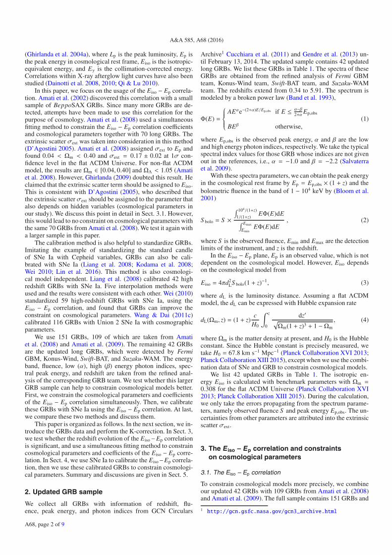
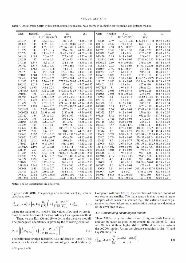
Fig. 3. Low-redshift GRM sample Eiso − Ep correlation. Black line isthe best-fit result obtained by using the bisector of the two ordinaryleast squares method. The dotted line represents the 1σext region anddashed line the 2σext region.
where zi+1 and zi are the redshift of the two nearest SNe Ia andεμ,i+1 and εμ,i are the errors of these two SNe Ia. The redshift ofinterpolated GRB lies between zi and zi+1.
After the distance moduli of 61 low-redshift GRBs are ob-tained, the luminosity distance can be derived from
μ = 5 logdL
Mpc+ 25. (9)
Then the isotropic-equivalent energy Eiso can be calculated fromEq. (3). Following Schaefer (2007) and Liang et al. (2008), weuse the bisector of the two ordinary least squares method (Isobeet al. 1990) to fit the Eiso − Ep correlation. The best-fit valuesare a = 48.46 ± 0.033 and b = 1.766 ± 0.007. The result isshown in Fig. 3. The errors of distance moduli are not takeninto consideration because the extrinsic scatter σext dominatesthe error size in the regression analysis (Schaefer 2007). Thus,we take σext directly into account during the calculations of theuncertainties of high-redshift GRBs (σlog Eiso ). From the previoussection, the value of σext is nearly constant, so we typically setσext = 0.34.
We have shown that the Eiso −Ep correlation does not evolvewith redshift in the previous section. Thus, the calibrated Eiso −Ep correlation can be extrapolated to the high-redshift sample,namely, z > 1.414 group. Using Eq. (5), we can derive Eiso of
A68, page 5 of 9
A&A 585, A68 (2016)
Table 4. 90 calibrated GRBs with redshift, bolometric fluence, peak energy in cosmological rest frame, and distance moduli.
GRB Redshift S bolo Ep μcal GRB Redshift S bolo Ep μcal
z (10−5 erg cm−2) (keV) z (10−5 erg cm−2) (keV)
050318 1.44 0.42 ± 0.03 115 ± 25 44.48 ± 1.28 130518 2.49 12.34 ± 0.08 1382.04 ± 31.41 45.96 ± 0.86100814 1.44 1.39 ± 0.23 312.32 ± 48.80 45.09 ± 1.11 081121 2.512 1.71 ± 0.33 871 ± 123 47.23 ± 1.08110213 1.46 1.55 ± 0.23 223.86 ± 70.11 44.34 ± 1.63 081118 2.58 0.27 ± 0.057 147 ± 14 45.84 ± 0.98010222 1.48 14.6 ± 1.5 766 ± 30 44.28 ± 0.88 080721 2.591 7.86 ± 1.37 1741 ± 227 46.92 ± 1.04120724 1.48 0.15 ± 0.02 68.45 ± 18.60 44.62 ± 1.48 050820 2.612 6.4 ± 0.5 1325 ± 277 46.63 ± 1.26060418 1.489 2.3 ± 0.5 572 ± 143 45.73 ± 1.41 030429 2.65 0.14 ± 0.02 128 ± 26 46.31 ± 1.25030328 1.52 6.4 ± 0.6 328 ± 55 43.56 ± 1.13 120811C 2.671 0.74 ± 0.07 157.49 ± 20.92 44.91 ± 1.04070125 1.547 13.3 ± 1.3 934 ± 148 44.79 ± 1.11 080603B 2.69 0.64 ± 0.058 376 ± 100 46.74 ± 1.45090102 1.547 3.48 ± 0.63 1149 ± 166 46.64 ± 1.08 140206A 2.73 1.69 ± 0.03 447.60 ± 22.38 46.03 ± 0.88040912 1.563 0.21 ± 0.06 44 ± 33 43.44 ± 3.43 091029 2.752 0.47 ± 0.044 230 ± 66 46.15 ± 1.53990123 1.6 35.8 ± 5.8 1724 ± 466 44.91 ± 1.48 081222 2.77 1.67 ± 0.17 505 ± 34 46.29 ± 0.91071003 1.604 5.32 ± 0.59 2077 ± 286 47.34 ± 1.05 050603 2.821 3.5 ± 0.2 1333 ± 107 47.36 ± 0.92090418 1.608 2.35 ± 0.59 1567 ± 384 47.69 ± 1.40 110731 2.83 2.51 ± 0.01 1164.32 ± 49.79 47.46 ± 0.87110503 1.613 2.76 ± 0.21 572.25 ± 50.95 45.58 ± 0.94 111107 2.893 0.18 ± 0.03 420.44 ± 124.58 48.39 ± 1.57990510 1.619 2.6 ± 0.4 423 ± 42 45.07 ± 0.97 050401 2.9 1.9 ± 0.4 467 ± 110 46.03 ± 1.36080605 1.6398 3.4 ± 0.28 650 ± 55 45.61 ± 0.93 090715B 3 1.09 ± 0.17 536 ± 172 46.93 ± 1.66131105A 1.686 4.75 ± 0.16 547.68 ± 83.53 44.94 ± 1.09 080607 3.036 8.96 ± 0.48 1691 ± 226 46.85 ± 1.04091020 1.71 0.11 ± 0.034 280 ± 190 47.75 ± 3.13 081028 3.038 0.81 ± 0.095 234 ± 93 45.67 ± 1.95100906 1.727 3.56 ± 0.55 387.23 ± 244.07 44.60 ± 2.91 120922 3.1 1.59 ± 0.18 156.62 ± 0.04 44.19 ± 0.86120119 1.728 4.62 ± 0.59 417.38 ± 54.56 44.46 ± 1.04 020124 3.2 1.2 ± 0.1 448 ± 148 46.53 ± 1.69110422 1.77 9.32 ± 0.02 421.04 ± 13.85 43.74 ± 0.86 060526 3.21 0.12 ± 0.06 105 ± 21 46.25 ± 1.34120326 1.798 0.44 ± 0.02 129.97 ± 10.27 44.81 ± 0.92 080810 3.35 1.82 ± 0.2 1470 ± 180 48.40 ± 1.02080514B 1.8 2.027 ± 0.48 627 ± 65 46.17 ± 1.00 110818 3.36 1.05 ± 0.08 1117.47 ± 241.11 48.47 ± 1.28090902B 1.822 32.38 ± 1.01 2187 ± 31 45.56 ± 0.85 030323 3.37 0.12 ± 0.04 270 ± 113 48.10 ± 2.07020127 1.9 0.38 ± 0.01 290 ± 100 46.55 ± 1.74 971214 3.42 0.87 ± 0.11 685 ± 133 47.75 ± 1.22080319C 1.95 1.5 ± 0.3 906 ± 272 47.26 ± 1.59 060707 3.425 0.23 ± 0.04 279 ± 28 47.47 ± 0.98081008 1.9685 0.96 ± 0.09 261 ± 52 45.36 ± 1.23 060115 3.53 0.25 ± 0.04 285 ± 34 47.45 ± 1.02030226 1.98 1.3 ± 0.1 289 ± 66 45.23 ± 1.32 090323 3.57 14.98 ± 1.83 1901 ± 343 46.65 ± 1.17130612 2.006 0.08 ± 0.01 186.07 ± 31.56 47.43 ± 1.14 100704 3.6 0.70 ± 0.07 809.60 ± 135.70 48.35 ± 1.13000926 2.07 2.6 ± 0.6 310 ± 20 44.65 ± 0.93 130514 3.6 1.88 ± 0.25 496.80 ± 151.80 46.34 ± 1.60130610 2.092 0.82 ± 0.05 911.83 ± 132.65 47.98 ± 1.07 130408 3.758 0.99 ± 0.17 1003.94 ± 137.98 48.42 ± 1.06090926 2.1062 15.08 ± 0.77 974 ± 50 44.95 ± 0.88 120802 3.796 0.43 ± 0.07 274.33 ± 93.04 46.85 ± 1.73011211 2.14 0.5 ± 0.06 186 ± 24 45.48 ± 1.03 100413 3.9 2.36 ± 0.77 1783.60 ± 374.85 48.61 ± 1.31071020 2.145 0.87 ± 0.4 1013 ± 160 48.13 ± 1.21 120909 3.93 2.69 ± 0.23 1651.55 ± 123.25 48.33 ± 0.92050922C 2.198 0.47 ± 0.16 415 ± 111 47.11 ± 1.50 131117A 4.042 0.05 ± 0.01 221.85 ± 37.31 48.83 ± 1.15121128 2.2 0.87 ± 0.07 243.20 ± 12.80 45.42 ± 0.89 060206 4.048 0.14 ± 0.03 394 ± 46 48.82 ± 1.02110205 2.22 3.32 ± 0.68 740.60 ± 322.00 46.10 ± 2.11 090516 4.109 1.96 ± 0.38 971 ± 390 47.70 ± 1.98130505 2.27 4.56 ± 0.09 2063.37 ± 101.37 47.74 ± 0.88 080916C 4.35 10.13 ± 2.13 2646 ± 566 47.88 ± 1.29060124 2.296 3.4 ± 0.5 784 ± 285 46.21 ± 1.82 000131 4.5 4.7 ± 0.8 987 ± 416 46.86 ± 2.05021004 2.3 0.27 ± 0.04 266 ± 117 46.89 ± 2.13 111008 5 1.06 ± 0.11 894.00 ± 240.00 48.38 ± 1.46051109A 2.346 0.51 ± 0.05 539 ± 200 47.57 ± 1.85 060927 5.6 0.27 ± 0.04 475 ± 47 48.76 ± 0.97060908 2.43 0.73 ± 0.07 514 ± 102 47.12 ± 1.23 130606 5.91 0.49 ± 0.09 2031.54 ± 483.70 50.94 ± 1.37080413 2.433 0.56 ± 0.14 584 ± 180 47.65 ± 1.63 050904 6.29 2 ± 0.2 3178 ± 1094 50.33 ± 1.75090812 2.452 3.077 ± 0.53 2000 ± 700 48.17 ± 1.77 080913 6.695 0.12 ± 0.035 710 ± 350 50.57 ± 2.36100728B 2.453 0.29 ± 0.01 359.11 ± 48.34 47.44 ± 1.04 090423 8.2 0.12 ± 0.032 491 ± 200 50.05 ± 2.01
Notes. The 1σ uncertainties are also given.
high-redshift GRBs. The propagated uncertainties of Eiso can becalculated from
σ2log Eiso
= σ2a +
(σb log
Ep
keV
)2
+
(b
ln 10
σEp
Ep
)2
+ σ2ext, (10)
where the value of σext is 0.34. The values of σa and σb are de-rived from the bisector of the two ordinary least squares method.
Then, we use Eqs. (3) and (9) to derive the distance moduli.The propagated uncertainty is given by the following equation:
σμ =
⎡⎢⎢⎢⎢⎢⎣(52σlog Eiso
)2
+
(5
2 ln 10
σS bolo
S bolo
)2⎤⎥⎥⎥⎥⎥⎦1/2
. (11)
The calibrated 90 high-redshift GRBs are listed in Table 4. Thissample can be used to constrain cosmological models directly.
Compared with Wei (2010), the error bars of distance moduli ofour results are smaller. The main reason is that we use a largersample, which leads to a smaller σext. The extrinsic scatter pa-rameter has been taken into consideration during the calculationof the error size of Eiso.
4.2. Constraining cosmological models
These GRBs carry the information of high-redshift Universe,and can be taken as good complements to the Union 2.1 dataset. We test if these high-redshift GRBs alone can constrainthe ΛCDM model. Using the distance modulus in Eq. (4) andEq. (9), the χ2 is
χ2GRB(Ωm) =
90∑i=1
[μcal(zi) − μ(zi)
]2
σ2(zi), (12)
A68, page 6 of 9
J. S. Wang et al.: Measuring dark energy with Eiso − Ep correlation
where μcal is the calibrated GRB distance modulus listed inTable 4. The best-fit result is Ωm = 0.23+0.06
−0.04 with 1σ uncer-tainty. The χ2 evolution withΩm is shown in Fig. 2. This result isconsistent with the constraints from SNe Ia (Conley et al. 2011;Suzuki et al. 2012), CMB (Planck Collaboration XVI 2013;Planck Collaboration XIII 2015), and BAO (Beutler et al. 2011;Anderson et al. 2014; Kazin et al. 2014; Ross et al. 2015) at 1σconfidence level, as shown in Table 3.
Since this GRB sample can constrain cosmological parame-ters successfully, we also combine the calibrated GRB data withSNe Ia from Union 2.1 sample to constrain cosmological mod-els. For the flat ΛCDM, we obtain Ωm = 0.271 ± 0.019 andh = 0.701 ± 0.002, where h is the Hubble constant in units of100 km s−1 Mpc−1. This is very consistent with the Union 2.1SNe Ia data. For the non-flat ΛCDM, the luminosity distance isdifferent and can be expressed as follows:
dL =
⎧⎪⎪⎪⎨⎪⎪⎪⎩cH−1
0 (1 + z)(−Ωk)−1/2 sin[(−Ωk)1/2I], Ωk < 0,cH−1
0 (1 + z)I, Ωk = 0,cH−1
0 (1 + z)Ω−1/2k sinh[Ω1/2
k I], Ωk > 0,(13)
where
Ωk = 1 − Ωm −ΩΛ, (14)
and
I =∫ z
0
dz√(1 + z)3Ωm + ΩΛ + (1 + z)2Ωk
· (15)
The χ2 of SNe Ia is constructed as follows:
χ2SNe(h,Ωm,ΩΛ) =
580∑i=1
[μobs(zi) − μ(zi)
]2
σ2(zi)· (16)
Then the total χ2 is
χ2total(h,Ωm,ΩΛ) = χ2
SNe(h,Ωm,ΩΛ) + χ2GRB(h,Ωm,ΩΛ)· (17)
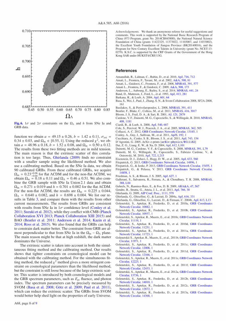
The best-fit values with 1σ uncertainties areΩm = 0.225±0.044,ΩΛ = 0.640 ± 0.082, and h = 0.698 ± 0.004 for the com-bined sample (SNe+GRB). For the GRB sample, we obtainΩm = 0.18±0.11 andΩΛ = 0.46±0.51, which is consistent withthe SNe Ia results at 1σ confidence level. The combined sam-ple can help to constrain cosmological parameters much tighterbecause not only is the sample enlarged, but also the redshiftcovers a much wider. The flatness of the Universe depends onthe curvature parameter, that is to say, Ωk = 1 − ΩΛ − Ωm.In Fig. 4, we use three samples, GRB, SNe, and combinationof GRB+SNe to constrain the cosmological model. Both resultsprefer a flat Universe at the 1σ confidence level. The constraintfrom the GRB is almost perpendicular to that from SNe Ia in theΩm − ΩΛ plane. Thus GRBs can significantly help to constrainΩm because, in this redshift domain, the dark matter dominatesthe evolution of the Universe. We also show constraints onΩm−hin Fig. 5, and ΩΛ − h in Fig. 6.
5. Discussions and summary
In this paper, we update 42 long GRBs for the Eiso − Ep corre-lation and combine them with 109 long GRBs from Amati et al.(2008) and Amati et al. (2009). This sample contains GRBs de-tected by different detectors with different sensitivities. Thus, thesample might be biased, but this bias should only have a weak
Flat Universe
GRB
GRB�SNe
SNe
0.0 0.1 0.2 0.3 0.4 0.50.0
0.2
0.4
0.6
0.8
1.0
1.2
�m��
Fig. 4. 1σ and 2σ constraints on Ωm and ΩΛ. We use three samples andplot them into different colors. The solid line shows the Ωk = 0 case.
0.15 0.20 0.25 0.300.685
0.690
0.695
0.700
0.705
�m
h
Fig. 5. 1σ and 2σ constraints on Ωm and h from SNe Ia and GRB data.
effect on our results. We also use the complete sample to per-form our analysis. We use the same criteria as Salvaterra et al.(2012) and Pescalli et al. (2015) to collect GRBs. The results area = 49.45 ± 0.61, b = 1.24 ± 0.22 and σext = 0.38 ± 0.06, whileno constraint on Ωm is found. These results are in tension withthat of our updated full sample with a larger extrinsic scatter. Nostatistical evidence for the redshift evolution of the Eiso − Ep isfound in the full sample.
For cosmological purposes, we fit the Eiso − Ep plane andthe cosmological parameters simultaneously. Using a likelihood
A68, page 7 of 9
A&A 585, A68 (2016)
0.45 0.50 0.55 0.60 0.65 0.70 0.75 0.80 0.850.685
0.690
0.695
0.700
0.705
0.710
��
h
Fig. 6. 1σ and 2σ constraints on the ΩΛ and h from SNe Ia andGRB data.
function we obtain a = 49.15 ± 0.26, b = 1.42 ± 0.11, σext =0.34 ± 0.03, and Ωm ∈ [0.55, 1]. Using the reduced χ2, we ob-tain a = 48.96 ± 0.18, b = 1.52 ± 0.08, and Ωm = 0.50 ± 0.12.The results from these two fitting methods are in mild tension.The main reason is that the extrinsic scatter of this correla-tion is too large. Thus, Ghirlanda (2009) finds no constraintwith a smaller sample using the likelihood method. We alsouse a calibrating method. Based on the SNe Ia data, we obtain90 calibrated GRBs. From these calibrated GRBs, we acquireΩm = 0.23+0.06
−0.04 for flat ΛCDM and for the non-flat ΛCDM, weobtain Ωm = 0.18 ± 0.11 and ΩΛ = 0.46 ± 0.51. We also com-bine the GRB sample with SNe Ia Union 2.1 data and obtainΩm = 0.271 ± 0.019 and h = 0.701 ± 0.002 for the flat ΛCDM.For the non-flat ΛCDM, the results are Ωm = 0.225 ± 0.044,ΩΛ = 0.640 ± 0.082, and h = 0.698 ± 0.004. We list our re-sults in Table 3, and compare them with the results from othercurrent measurements. The results from GRBs are consistentwith results from SNe Ia in 1σ confidence level (Conley et al.2011; Suzuki et al. 2012), while they conflict with CMB (PlanckCollaboration XVI 2013; Planck Collaboration XIII 2015) andBAO (Beutler et al. 2011; Anderson et al. 2014; Kazin et al.2014; Ross et al. 2015). We also found that the GRBs can helpto constrain dark matter better. The constraint from GRB are al-most perpendicular to that from SNe Ia in the Ωm − ΩΛ plane.The main reason might be that at high redshift, the dark matterdominates the Universe.
The extrinsic scatter is taken into account in both the simul-taneous fitting method and the calibrating method. Our resultsshows that tighter constraints on cosmological model can beobtained with the calibrating method. For the simultaneous fit-ting method, the reduced χ2 method gives a more stringent con-straint on cosmological parameters than the likelihood method,but the constraint is still loose because of the large extrinsic scat-ter. This scatter is introduced by both cosmological models andthe GRB spectrum parameters, such as Ep, fluence, and photonindex. The spectrum parameters can be precisely measured bySVOM (Basa et al. 2008; Götz et al. 2009; Paul et al. 2011),which can reduce the extrinsic scatter. The GRBs from SVOMwould better help shed light on the properties of early Universe.
Acknowledgements. We thank an anonymous referee for useful suggestions andcomments. This work is supported by the National Basic Research Program ofChina (973 Program, grant No. 2014CB845800), the National Natural ScienceFoundation of China (grants 11422325, 11373022, 11103007, and 11033002),the Excellent Youth Foundation of Jiangsu Province (BK20140016), and theProgram for New Century Excellent Talents in University (grant No. NCET-13-0279). K.S.C. is supported by the CRF Grants of the Government of the HongKong SAR under HUKST4/CRF/13G.
ReferencesAmanullah, R., Lidman, C., Rubin, D., et al. 2010, ApJ, 716, 712Amati, L., Frontera, F., Tavani, M., et al. 2002, A&A, 390, 81Amati, L., Guidorzi, C., Frontera, F., et al. 2008, MNRAS, 391, 577Amati L., Frontera, F., & Guidorzi, C. 2009, A&A, 508, 173Anderson, L., Aubourg, É., Bailey, S., et al. 2014, MNRAS, 441, 24Band, D., Matteson, J., Ford, L., et al. 1993, ApJ, 413, 281Barkana, R., & Loeb, A. 2004, ApJ, 601, 64Basa, S., Wei, J., Paul, J., Zhang, S. N., & Svom Collaboration 2008, SF2A-2008,
161Basilakos, S., & Perivolaropoulos, L. 2008, MNRAS, 391, 411Beutler, F., Blake, C., Colless, M., et al. 2011, MNRAS, 416, 3017Bloom, J. S., Frail, D. A., & Sari, R. 2001, AJ, 121, 2879Cardone, V. F., Dainotti, M. G., Capozziello, S., & Willingale, R. 2010, MNRAS,
408, 1181Ciardi, B., & Loeb, A. 2000, ApJ, 540, 687Cole, S., Percival, W. J., Peacock, J. A., et al. 2005, MNRAS, 362, 505Collazzi, A. C. 2012, GRB Coordinates Network Circular, 13145, 1Conley, A., Guy, J., Sullivan, M., et al. 2011, ApJS, 192, 1Cucchiara, A., Cenko, S. B., Bloom, J. S., et al. 2011, ApJ, 743, 154D’Agostini, G. 2005, ArXiv e-prints [arXiv:physics/0511182]Dai, Z. G., Liang, E. W., & Xu, D. 2004, ApJ, 612, L101Dainotti, M. G., Cardone, V. F., & Capozziello, S. 2008, MNRAS, 391, L79Dainotti, M. G., Willingale, R., Capozziello, S., Fabrizio Cardone, V., &
Ostrowski, M. 2010, ApJ, 722, L215Eisenstein, D. J., Zehavi, I., Hogg, D. W., et al. 2005, ApJ, 633, 560Fitzpatrick, G. 2013, GRB Coordinates Network Circular, 14896, 1Fitzpatrick, G., & Jenke, P. 2013, GRB Coordinates Network Circular, 15455, 1Fitzpatrick, G., & Pelassa, V. 2013, GRB Coordinates Network Circular,
14858, 1Friedman, A. S., & Bloom, J. S. 2005, ApJ, 627, 1Gallerani, S., Salvaterra, R., Ferrara, A., & Choudhury, T. R. 2008, MNRAS,
388, L84Gehrels, N., Ramirez-Ruiz, E., & Fox, D. B. 2009, ARA&A, 47, 567Gendre, B., Stratta, G., Atteia, J. L., et al. 2013, ApJ, 766, 30Ghirlanda, G. 2009, AIP Conf. Proc., 1111, 579Ghirlanda, G., Ghisellini, G., & Lazzati, D. 2004a, ApJ, 616, 331Ghirlanda, G., Ghisellini, G., Lazzati, D., & Firmani, C. 2004b, ApJ, 613, L13Golenetskii, S., Aptekar, R., Frederiks, D., et al. 2010a, GRB Coordinates
Network Circular, 10882, 1Golenetskii, S., Aptekar, R., Frederiks, D., et al. 2010b, GRB Coordinates
Network Circular, 10937, 1Golenetskii, S., Aptekar, R., Mazets, E., et al. 2010c, GRB Coordinates Network
Circular, 11119, 1Golenetskii, S., Aptekar, R., Frederiks, D., et al. 2010d, GRB Coordinates
Network Circular, 11251, 1Golenetskii, S., Aptekar, R., Frederiks, D., et al. 2011a, GRB Coordinates
Network Circular, 11723, 1Golenetskii S., Aptekar, R., Mazets, E., et al., 2011b, GRB Coordinates Network
Circular, 11971, 1Golenetskii, S., Aptekar, R., Frederiks, D., et al. 2011c, GRB Coordinates
Network Circular, 12008, 1Golenetskii, S., Aptekar, R., Frederiks, D., et al. 2011d, GRB Coordinates
Network Circular, 12166, 1Golenetskii, S., Aptekar, R., Mazets, E., et al. 2011e, GRB Coordinates Network
Circular, 12223, 1Golenetskii, S., Aptekar, R., Frederiks, D., et al. 2011f, GRB Coordinates
Network Circular, 12433, 1Golenetskii, S., Aptekar, R., Mazets, E., et al. 2012a, GRB Coordinates Network
Circular, 13736, 1Golenetskii, S., Aptekar, R., Frederiks, D., et al. 2012b, GRB Coordinates
Network Circular, 14010, 1Golenetskii, S., Aptekar, R., Frederiks, D., et al. 2012c, GRB Coordinates
Network Circular, 12872, 1Golenetskii, S., Aptekar, R., Frederiks, D., et al. 2013a, GRB Coordinates
Network Circular, 14368, 1
A68, page 8 of 9
J. S. Wang et al.: Measuring dark energy with Eiso − Ep correlation
Golenetskii, S., Aptekar, R., Frederiks, D., et al. 2013b, GRB CoordinatesNetwork Circular, 14487, 1
Golenetskii, S., Aptekar, R., Frederiks, D., et al. 2013c, GRB CoordinatesNetwork Circular, 14575, 1
Golenetskii, S., Aptekar, R., Mazets, E., et al. 2013d, GRB Coordinates NetworkCircular, 14808, 1
Golenetskii, S., Aptekar, R., Frederiks, D., et al. 2013e, GRB CoordinatesNetwork Circular, 14958, 1
Golenetskii, S., Aptekar, R., Frederiks, D., et al. 2013f, GRB CoordinatesNetwork Circular, 15145, 1
Golenetskii, S., Aptekar, R., Frederiks, D., et al. 2013g, GRB CoordinatesNetwork Circular, 15203, 1
Golenetskii, S., Aptekar, R., Frederiks, D., et al. 2013h, GRB CoordinatesNetwork Circular, 15413, 1
Götz, D., Paul, J., Basa, S., et al. 2009, AIP Conf. Ser., 1133, 25Isobe, T., Feigelson, E. D., Akritas, M. G., & Babu, G. J. 1990, ApJ, 364, 104Kazin, E. A., Koda, J., Blake, C., et al. 2014, MNRAS, 441, 3524Kodama, Y., Yonetoku, D., Murakami, T., et al. 2008, MNRAS, 391, L1Komatsu, E., Smith, K. M., Dunkley, J., et al. 2011, ApJS, 192, 18Kowalski, M., Rubin, D., Aldering, G., et al. 2008, ApJ, 686, 749Krimm, H. A., Barthelmy, S. D., Baumgartner, W. H., et al. 2012a, GRB
Coordinates Network Circular, 13517, 1Krimm, H. A., Barlow, B. N., Barthelmy, S. D., et al. 2012b, GRB Coordinates
Network Circular, 13634, 1Krimm, H. A., Barthelmy, S. D., Baumgartner, W. H., et al. 2012c, GRB
Coordinates Network Circular, 13806, 1Krimm, H. A., Barthelmy, S. D., Baumgartner, W. H., et al. 2013, GRB
Coordinates Network Circular, 15499, 1Lamb, D. Q., & Reichart, D. E. 2000, ApJ, 536, 1Li, M.-H., & Lin, H.-N. 2015, ApJ, 807, 76Liang, E., & Zhang, B. 2005, ApJ, 633, 611Liang, N., Xiao, W. K., Liu, Y., & Zhang, S. N. 2008, ApJ, 685, 354Lin, H.-N., Li, X., & Change, Z. 2016, MNRAS, 455, 2131Mészáros, P. 2006, Rep. Prog. Phys., 69, 2259Palshin, V., et al. 2013, GRB Coordinates Network Circular, 14702, 1Paul, J., Wei, J., Basa, S., & Zhang, S.-N. 2011, Comptes Rendus Physique, 12,
298Pelassa, V. 2011, GRB Coordinates Network Circular, 12545, 1Perlmutter, S., Aldering, G., Goldhaber, G., et al. 1999, ApJ, 517, 565Pescalli, A., Ghirlanda, G., Salvaterra, R., et al. 2015, A&A, submitted
[arXiv:1506.05463v1]Planck Collaboration XVI. 2014, A&A, 571, A16Planck Collaboration XIII. 2015, A&A, submitted [arXiv:1502.01589]
Porciani, C., & Madau, P. 2001, ApJ, 548, 522Qi, S., & Lu, T. 2010, ApJ, 717, 1274Qi, S., Lu, T., & Wang, F.-Y. 2009, MNRAS, 398, L78Riess, A. G., Filippenko, A. V., Challis, P., et al. 1998, AJ, 116, 1009Ross, A. J., Samushia, L., Howlett, C., et al. 2015, MNRAS, 449, 835Salvaterra, R., Della Valle, M., Campana, S., et al. 2009, Nature, 461, 1258Salvaterra, R., Campana, S., Vergani, S. D., et al. 2012, ApJ, 749, 68Schaefer, B. E. 2003, ApJ, 583, L67Schaefer, B. E. 2007, ApJ, 660, 16Stamatikos, M., Barthelmy, S. D., Baumgartner, W. H., et al. 2012, GRB
Coordinates Network Circular, 13559, 1Sugita, S., Yamaoka, K., Ohno, M., et al. 2010, GRB Coordinates Network
Circular, 10604, 1Suzuki, N., Rubin, D., Lidman, C., et al. 2012, ApJ, 746, 85Tanvir, N. R., Fox, D. B., Levan, A. J., et al. 2009, Natur, 461, 1254Totani, T. 1997, ApJ, 486, L71Totani, T., Kawai, N., Kosugi, G., et al. 2006, PASJ, 58, 485von Kienlin, A. 2010, GRB Coordinates Network Circular, 11015, 1von Kienlin, A. 2013, GRB Coordinates Network Circular, 14473, 1von Kienlin, A., & Bhat, P. N. 2014, GRB Coordinates Network Circular,
15796, 1Wang, F. Y. 2012, A&A, 543, A91Wang, F. Y. 2013, A&A, 556, A90Wang, F. Y., & Dai, Z. G. 2009, MNRAS, 400, L10Wang, F. Y., & Dai, Z. G. 2011a, ApJ, 727, L34Wang, F. Y., & Dai, Z. G. 2011c, A&A, 536, A96Wang, F. Y., & Dai, Z. G. 2014, Phys. Rev. D, 89, 023004Wang, F. Y., Dai, Z. G., & Zhu, Z.-H. 2007, ApJ, 667, 1Wang, F.-Y., Qi, S., & Dai, Z.-G. 2011, MNRAS, 415, 3423Wang, F. Y., Bromm, V., Greif, T. H., et al. 2012, ApJ, 760, 27Wang, F. Y., Dai, Z. G., & Liang, E. W. 2015, New Astron. Rev., 67, 1Wang, J. S., & Wang, F. Y. 2014a, MNRAS, 443, 1680Wang, J. S., & Wang, F. Y. 2014b, A&A, 564, A137Wei, D. M., & Gao, W. H. 2003, MNRAS, 345, 743Wei, H. 2010, JCAP, 8, 20Wijers, R. A. M. J., Bloom, J. S., Bagla, J. S., & Natarajan, P. 1998, MNRAS,
294, L13Xiong, S. 2011, GRB Coordinates Network Circular, 12287, 1Xiong, S. 2013, GRB Coordinates Network Circular, 14674, 1Xiong, S., & Rau, A. 2013, GRB Coordinates Network Circular, 14429, 1Younes, G., & Bhat, P. N. 2013, GRB Coordinates Network Circular, 14219, 1Zhang, B. 2007, Chin. J. Astron. Astrophys., 7, 1Zhang, B. B. 2014, GRB Coordinates Network Circular, 15833, 1
A68, page 9 of 9