Measuring Conditional Party Government*

by

John H. AldrichDuke University

and

David W. RohdeMichigan State University

*Prepared for delivery at the Annual Meeting of the Midwest Political Science Association,Palmer House Hotel, Chicago, Ill., April 23-25, 1998. We would like to thank Jim Battista,Adam Frey, Beatriz Magloni, and Lynn Van Scoyoc for their assistance. We bear fullresponsibility for the contents of this paper.

2

Abstract

Measuring Conditional Party Government

by

John H. AldrichDuke University

and

David W. RohdeMichigan State University

In this paper, we extend our theory and measurement of conditional party government.

We define the “condition” in conditional party government more precisely, offering a formal

illustration that indicates how, when the condition is more rather than less well satisfied, the

majority party may skew outcomes from the center of the floor toward the center of their party.

We then provide a number of measures designed to illustrate variation in the degree to which this

condition has been satisfied in post-War Congresses. The evidence suggests that the condition

was relatively more fully satisfied in the early post-War years, its degree of satisfaction declined

in the 1960s and 1970s, from which point its degree of satisfaction increased. By the mid-1990s,

the condition was at a (relative) peak of satisfaction. Finally, we examine variations over time in

two variables concerning the intra-legislative party to provide at least a preliminary indication

whether partisan rules and powers might have been used to achieve majority party preferred

outcomes. As our theory predicts, their use increased as the degree to which the condition was

satisfied increased.

3

Measuring Conditional Party Government

Introduction

Shepsle (1989) employed the metaphor of the “textbook” Congress to describe a set of

beliefs held by congressional scholars about the patterns of structure, process, and outcomes

characteristic of the Congress (usually the House) at any given time. His use of the term was in

an account of how this textbook view can change, and in the case illustrated had changed. Thus,

in the 1950s and 1960s, the textbook view of structure was that of a House dominated by

geography and committees, with party hovering in the background. More recently, the House

has seen the party move more to share the foreground with geography, while the importance of

committees has receded somewhat.

In our prior work (1996a; 1996b; 1997; 1997-98), we have made comparable arguments

about the changing importance of various features of the House. Most especially, we have

argued that the relative importance of the political party in the Congress has waxed and waned.

Following Rohde (1991), we have called the account “conditional party government,” and we

have suggested that the importance of party varies with the degree to which the condition in

conditional party government is satisfied. In this paper, we seek to develop ways to measure this

condition and its changing degrees of satisfaction over the time, specifically over the 25

congresses of the post-War era. To do this, we need to define conditional party government

more precisely, and we offer here two propositions (one new, one from 1997b) that illustrate the

concept. We then develop a measurement strategy and apply it to these 25 congresses. We

complete the account by comparing the resulting variation in the apparent strength of conditional

4

party government to several measures of the use of the procedures of the House to implement

party positions. We hasten to add, however, that our theory is predicated on an understanding

that the importance of party will vary over time, but that the importance of the party, and use of

resources held by the party, will vary cross-sectionally. That is, there will be predictable patterns

in the degree to which the party leadership uses its powers and resources on different types of

legislation within the same Congress. We reserve that inquiry, however, for another paper.

Theory

The theory of conditional party government begins with the policy preferences Members

bring with them to the House and which they would choose to reveal in voting and other policy-

making actions. These preferences may contain a healthy component of the Member’s personal

views. Indeed, many Members entered politics in the first place because of their policy beliefs.

Still, a second, potentially independent source of a Member’s policy preferences, and an

explanation of why a Member with these particular policy views (if he or she has them) was

chosen in the first place, is the electoral process. Thus implicated are the preferences of the

Member’s core, primary, election-reelection, and geographic constituencies, resource providers,

etc.

Members’ behavior, we assume, may also be shaped to a considerable degree by the

legislative party. Parties as electoral institutions likely have a larger impact on behavior,

presumably revealed primarily in their effect on the preferences the Members bring with them to

the Congress, but we take these electoral forces as exogenous for our purposes here. We do

5

assume, in addition, that the parties may have considerable effect on Members’ behavior through

their partisan legislative institutions. Further, the relative effectiveness of the party as a

legislative institution is partially endogenous. It is endogenous to the degree to which the

condition in conditional party government is satisfied. This degree of satisfaction is, we

presume, due to electoral forces and/or ideological commitments of the candidates. That is, the

electoral and internal, legislative party are closely related.

The condition in conditional party government concerns the distribution of policy

preferences in the two parties. It is increasingly well satisfied the more homogenous the

preferences of Members are within each party (especially the majority party), and the more

different the preferences are between the two parties’ Members. The more one party agrees that

it wants outcomes that are different from those desired by the opposition, the more the condition

is satisfied.

Three sets of consequences flow from the increasing degree to which this condition is

satisfied. First, Members of a party are increasingly likely to chose to provide their legislative

party institutions and party leadership with stronger rules and with greater resources, the greater

the degree to which the condition is met. Second, the party will be expected to employ those

powers and resources more often, the greater the satisfaction of the condition. Third, provided

that the majority party has, by virtue of its being the majority party that organizes the House,

more powers and resources to employ than the minority party, then legislation should reveal that

fact. In particular, the greater the degree of satisfaction of the condition in conditional party

government, the farther policy outcomes should be skewed from the center of the whole

6

Congress toward the center of opinion in the majority party. This policy consequence can be

seen as a tug-of-war between the policy center of the House as a whole that, even in multi-

dimensional policy spaces, likely exerts considerable centripetal tendencies. Countering that

force is the centrifugal pull towards the center of the majority party, a centrifugal force that

should increase with increasing strength of the majority party.

Two Formal Illustrations

A Unidimensional Example of Conditional Party Government: Aldrich (1995) claimed

that, if the policy space is effectively unidimensional, then there would be no incentives for party

formation. To the contrary, we earlier demonstrated (1997) that, at least given that there are two

parties, there still may be incentives for Members to strengthen the legislative party in a

unidimensional policy world. These incentives will increase as the degree of satisfaction of the

condition in conditional party government increases. This case is one of the empowerment of a

collective organization to provide collective goods more effectively. Thus, it is concerned with

situations in which all in the party can be made better off by acting collectively and by choosing

some option closer to the center of the party than toward the center of the floor.1 Non-organized,

individual choices would result in simple, direct spatial voting and thus would lead to the median

voter result applying. If instead, the majority party caucused at the outset, they could thereby

realize (if true) that there were potential collective gains to be made. They could achieve those

gains by contributing powers and resources to the collective agents (the party leadership) of the

party. We then show in a simple illustration that all members of the majority party can be made

better off contributing and re-allocating to compensate marginal (moderate) members for voting

7

for options closer to the center of the party than by voting the party affiliates’ individual

preferences.

A Two-Dimensional Example of Conditional Party Government: The following two-

dimensional example provides an even clearer illustration of the workings of conditional party

government and the nature of the condition, doing so purely within the spatial voting theory

context.2 Consider a three-person legislature, with two members of the majority party (r1 and r2)

and one minority party member (d1). Let us begin with the distribution of ideal points that would

be the farthest from satisfying the condition in conditional party government. In particular, let

the ideal points be at the vertices of an equilateral triangle. Thus there is no greater commonality

of preferences between the members of party r than either have with party d’s representative.

Suppose that each representative has preferences that decline linearly with increasing distance

(simple Euclidean or “Type I” utility). Thus, nothing distinguishes members of this simple

legislature but their party label. Finally, let the status quo point (xs) be at the exact center of the

triangle (see Figure 1).3

In accord with Aldrich (1994), let the majority party be able to propose a bill, and the

minority party be able to propose an amendment (with agenda control possible through, for

example, control of committees and their chairs). The bill must be able to pass, of course, and it

also must make (at least a majority in) the majority party better off, or they would not propose it.

The amendment must do likewise for the minority party. That is the amendment must be

feasible (it will pass by beating the bill and the status quo), and it must be desirable (the minority

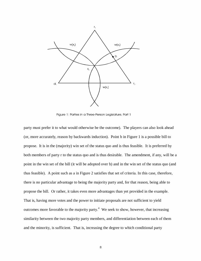
8

party must prefer it to what would otherwise be the outcome). The players can also look ahead

(or, more accurately, reason by backwards induction). Point b in Figure 1 is a possible bill to

propose. It is in the (majority) win set of the status quo and is thus feasible. It is preferred by

both members of party r to the status quo and is thus desirable. The amendment, if any, will be a

point in the win set of the bill (it will be adopted over b) and in the win set of the status quo (and

thus feasible). A point such as a in Figure 2 satisfies that set of criteria. In this case, therefore,

there is no particular advantage to being the majority party and, for that reason, being able to

propose the bill. Or rather, it takes even more advantages than yet provided in the example.

That is, having more votes and the power to initiate proposals are not sufficient to yield

outcomes more favorable to the majority party.4 We seek to show, however, that increasing

similarity between the two majority party members, and differentiation between each of them

and the minority, is sufficient. That is, increasing the degree to which conditional party

9

government is satisfied yields outcomes that do benefit the majority at the expense of the

minority.

Let the equilateral triangle become an isosceles triangle, with the ideal points of members of

party r relatively closer together and thereby being relatively farther from that of the minority

party member, as in Figure 3. Figure 3 was drawn so that the win set of xs and the win set of b

no longer overlap. Put alternatively, there is no longer an amendment that d1 can offer that both

defeats b (i.e., that she can get a member of party r to support with her) and defeats the status

quo.5 Thus, if party r proposes b, it is feasible and, for them, desirable to the status quo, and the

minority party has no amendment to offer to make anyone in party r better off. Thus, as the

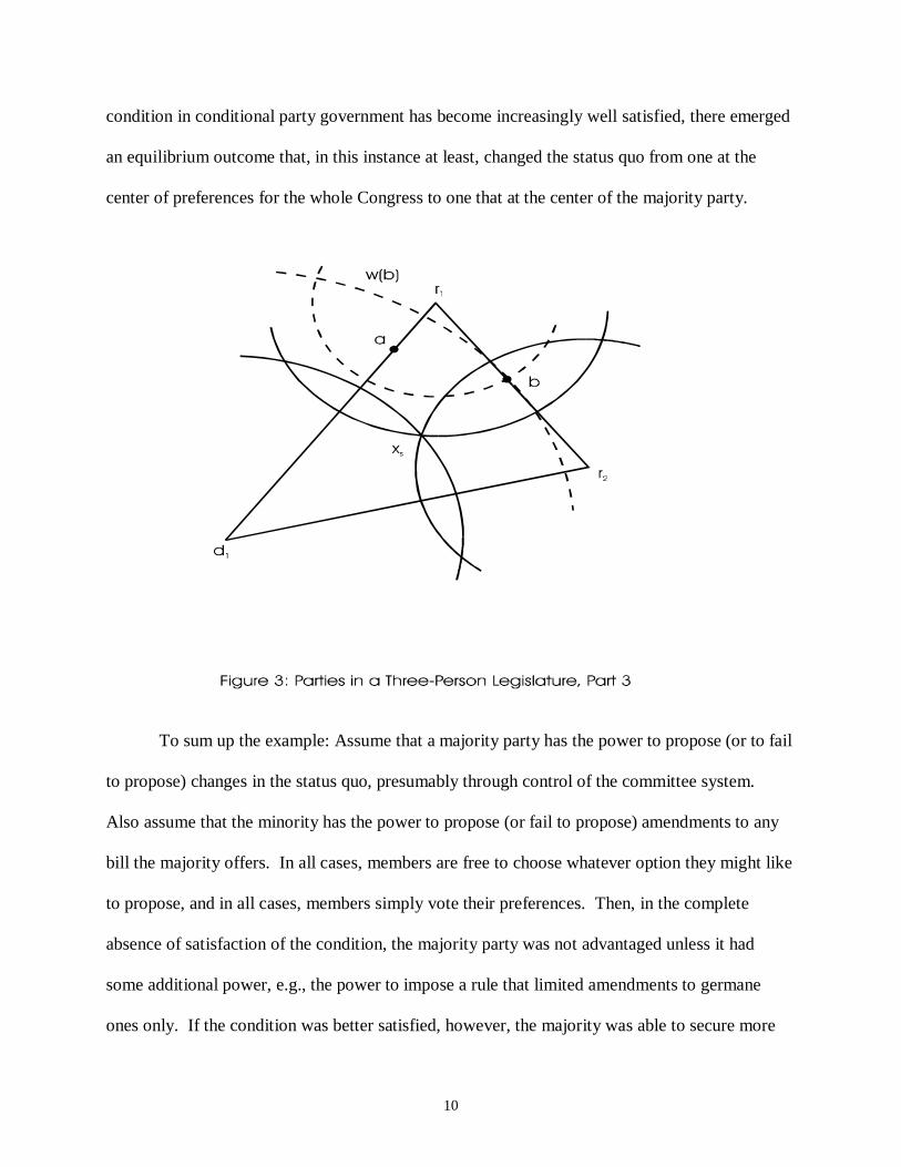
10

condition in conditional party government has become increasingly well satisfied, there emerged

an equilibrium outcome that, in this instance at least, changed the status quo from one at the

center of preferences for the whole Congress to one that at the center of the majority party.

To sum up the example: Assume that a majority party has the power to propose (or to fail

to propose) changes in the status quo, presumably through control of the committee system.

Also assume that the minority has the power to propose (or fail to propose) amendments to any

bill the majority offers. In all cases, members are free to choose whatever option they might like

to propose, and in all cases, members simply vote their preferences. Then, in the complete

absence of satisfaction of the condition, the majority party was not advantaged unless it had

some additional power, e.g., the power to impose a rule that limited amendments to germane

ones only. If the condition was better satisfied, however, the majority was able to secure more

11

collectively and move outcomes quite far from the center. This circumstance differs from a

decision due to preferences alone, because of the agenda control powers held by the majority.

There are two distinct situations in which the distribution of preferences in Figure 1

increasingly satisfies the condition. One is as drawn in Figure 3, that is, when elections select

majority party members whose ideal points are located closer to those of their partisans than to

the opposition. A second and potentially distinctive case is when ideal preferences are, as in

Figure 1, distributed such that there is no intra-party homogeneity, but in which all members

share a weighting of the dimensions that differs from equal saliency of the two dimensions. In

particular, consider the hypothetical line passing through d1 and b. This line is the dimension of

party cleavage, that is, the dimension that distinguished the preferences of members of party r

from those of members of party d. The second dimension runs through the ideal points of the

two members of the majority party and is, thus, the line of division within the majority party. If

ideal points are distributed as in Figure 1 but the party cleavage dimension is weighted more

heavily in all members’ utility functions, then Figure 1 with unequal saliency is identical to the

case in Figure 3, and party d has no feasible amendment it would desire to offer.6 This weighting

of partisan cleavages more strongly than intra-party divisions is a likely consequence of

elections, as well. After all, the general election is fought between candidates of the two parties,

so that the campaigns are likely to “prime” the electorate to consider party cleavages more

important. Thus, elections could induce satisfaction of the condition either through affecting the

distribution of ideal points, or shaping the importance of dimensions, or both.

12

Measuring the Variation in Conditional Party Government over Time

Measuring the Condition, per se: In this section we report some measures of the degree

to which the condition in conditional party government has been satisfied in the U.S. House.7

We do not offer an absolute measure, permitting us, for example, to say that the condition is 83%

satisfied. We are, however, able to compare variation in these measures over the post-War era

(more accurately, from the 80th through the 104th Congresses). We would ideally like an

exogenously determined measure of Member’s preferences. Many use estimated ideal point

positions from the procedure developed by Poole and Rosenthal (1985; 1997), and we will do so

here, as well. We have also performed all analyses on an alternative method recently developed

by Heckman and Snyder (1997; see also Snyder and Groseclose, 1997).

Krehbiel has recently (1998) critiqued the use of voting based measures of party, such as

party unity scores and the like. What we perceive to be the central claims of his argument in that

work should apply in at least some measure to these two measures (which we refer to as the

Poole and the Snyder data, for convenience). In our way of putting the argument, these ideal

point estimates are based on votes taken at the end of the democratic (i.e., electoral and

legislative) process. Thus, these measures of roll call voting include within their determination

all those elements that go into the preferences MC’s would like to express in voting (their own

preferences, those induced by constituents, etc.). But they also include the impact, if any, of

institutional structure, whether norms induced by, say, committee structures, effects of partisan

actions within the House, the consequences from bicameralism, and/or the influence of the

president. Any one set of observations, such as roll call votes, must therefore be considered a

13

complex mix of preferences and institutional considerations, inter alia. For purposes of this

section, however, we will follow convention and consider them as close to measures of

preference as can be obtained systematically. We will return to these considerations in the next

section.

We therefore use as our basic data the ideal point locations, as estimated by Poole and

Snyder, from their respective first dimensions.8 In both cases, that first dimension is the one

most closely associated with party cleavages.9 We then have developed a number of summary

measures based on the distribution of ideal points for all Members and the distributions of each

party’s affiliates. The full distributions of ideal point estimates by party for each of the 25

Congresses are reproduced in an Appendix (available in the on-line version of this paper, as well

as being available upon request).

We report the distribution over time of the following measures (in no particular order):

1. The difference between the location of the median Democrat and the median

Republican.10 This measure gets at one aspect of inter-party heterogeneity.

2. The ratio of the standard deviation of ideal points in the Democratic party to that of

the full House, which indicates variation in intra-party homogeneity.11

3. The proportion of overlap between the two parties’ distribution of ideal points

subtracted from one. Overlap is measured by the minimum number of ideal points

that would have to be changed to yield a complete separation of the two parties, with

all Democrats’ ideal points being to the left of all Republicans’ ideal points.

14

4. The R2 resulting from regressing the Member’s ideal point location on party

affiliation.

Each of these tap different aspects of the condition, and collectively they cumulate to a

reasonably full picture of how well or poorly the condition is satisfied in each Congress.

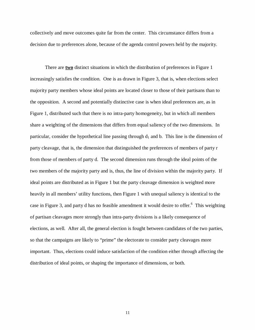
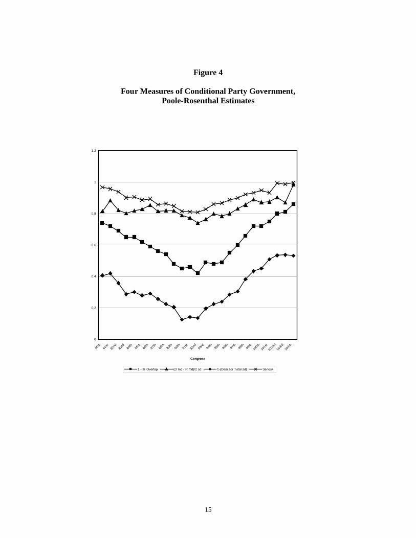
These mesures are reported in Figures 4 and 5, for the Poole and Snyder data,

respectively. While these two sets of estimates are not identical, they share a basic structure that

is visually evident in all four measures. The condition was at a relatively high degree of

satisfaction in the late 1940s and early 1950s. This degree of satisfaction slumped in the late

1960s and into the 1970s. It began to climb again in the 1980s and returned to another relative

high point from about the 100th Congress through the 104th Congress. The decline appears a bit

sharper in the Snyder data. Perhaps the R2 measure is most easily comparable. In Snyder, it

goes from the .9 ranges, dropping to .31 in the 91st Congress, and returning to the .9 levels at the

end. With the Poole estimates, the variation is from .74 in the 80th Congress, dropping to .42 in

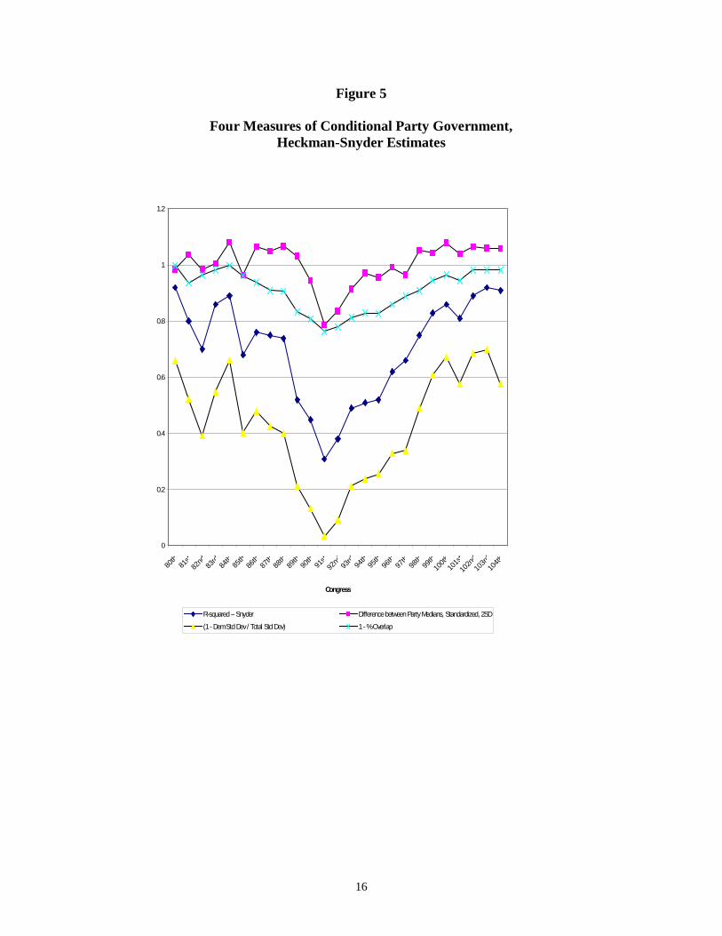
the 92nd Congress, and then climbing to .86 in the 104th Congress. Just what these numbers

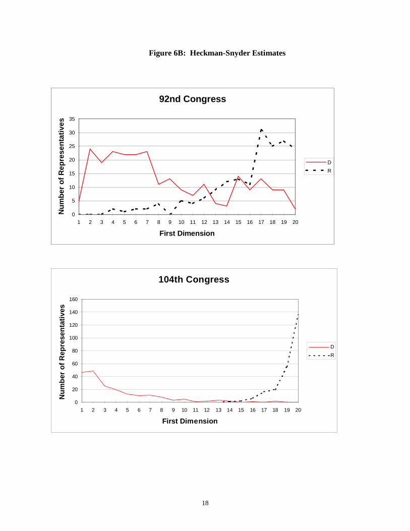
mean can perhaps best be appreciated by a visual representation. In Figure 6A, we reproduce the

distribution of ideal points as estimated by Poole and Rosenthal for their first dimension for two

Congresses, while 6B contains comparable reporting for the Heckman-Snyder data. One of the

two Congresses is the 92nd, that is among the most heterogeneous cases for ideal points among

the majority party, while the other is the 104th, in which the condition is as well approximated as

in any other post-War Congress. The ideal point positions were collapsed into 20 equal units to

illustrate the frequency distributions.

15

Figure 4

Four Measures of Conditional Party Government,Poole-Rosenthal Estimates

0

0.2

0.4

0.6

0.8

1

1.2

8

0th

81st

82nd

83r

d

84th

8

5th

8

6th

87th

8

8th

8

9th

9

0th

91st

92n

d

9

3rd

9

4th

9

5th

9

6th

9

7th

9

8th

9

9th

1

00th

1

01st

1

02nd

1

03rd

1

04th

Congress

1 - % Overlap (D md - R md)/2 sd 1-(Dem sd/ Total sd) Series4

16

Figure 5

Four Measures of Conditional Party Government,Heckman-Snyder Estimates

0

0.2

0.4

0.6

0.8

1

1.2

8

0th

81st

82nd

83r

d

84th

8

5th

8

6th

87th

8

8th

8

9th

9

0th

91st

92n

d

9

3rd

9

4th

9

5th

9

6th

9

7th

9

8th

9

9th

1

00th

1

01st

1

02nd

1

03rd

1

04th

Congress

R-squared -- Snyder Difference between Party Medians, Standardized, 2SD

(1 - Dem Std Dev / Total Std Dev) 1 - % Overlap

17

Figure 6

Distributions of Members’ Preferences byParty in the 92nd and 104th Congresses

Figure 6A: Poole-Rosenthal Estimates

92nd Congress

0

10

20

30

40

50

60

1 2 3 4 5 6 7 8 9 10 11 12 13 14 15 16 17 18 19 20

First Dimension

Nu

mb

er o

f R

epre

sen

tati

ves

D

R

104th Congress

0

10

20

30

40

50

60

70

1 2 3 4 5 6 7 8 9 10 11 12 13 14 15 16 17 18 19 20

First Dimension

Nu

mb

er o

f R

epre

sen

tati

ves

D

R

18

Figure 6B: Heckman-Snyder Estimates

92nd Congress

0

5

10

15

20

25

30

35

1 2 3 4 5 6 7 8 9 10 11 12 13 14 15 16 17 18 19 20

First Dimension

Nu

mb

er o

f R

epre

sen

tati

ves

D

R

104th Congress

0

20

40

60

80

100

120

140

160

1 2 3 4 5 6 7 8 9 10 11 12 13 14 15 16 17 18 19 20

First Dimension

Nu

mb

er o

f R

epre

sen

tati

ves

D

R

19

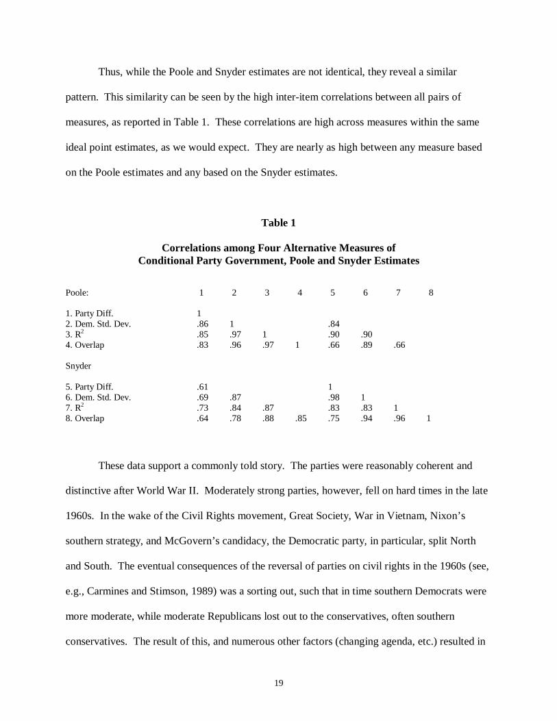
Thus, while the Poole and Snyder estimates are not identical, they reveal a similar

pattern. This similarity can be seen by the high inter-item correlations between all pairs of

measures, as reported in Table 1. These correlations are high across measures within the same

ideal point estimates, as we would expect. They are nearly as high between any measure based

on the Poole estimates and any based on the Snyder estimates.

Table 1

Correlations among Four Alternative Measures ofConditional Party Government, Poole and Snyder Estimates

Poole: 1 2 3 4 5 6 7 8

1. Party Diff. 12. Dem. Std. Dev. .86 1 .843. R2 .85 .97 1 .90 .904. Overlap .83 .96 .97 1 .66 .89 .66

Snyder

5. Party Diff. .61 16. Dem. Std. Dev. .69 .87 .98 17. R2 .73 .84 .87 .83 .83 18. Overlap .64 .78 .88 .85 .75 .94 .96 1

These data support a commonly told story. The parties were reasonably coherent and

distinctive after World War II. Moderately strong parties, however, fell on hard times in the late

1960s. In the wake of the Civil Rights movement, Great Society, War in Vietnam, Nixon’s

southern strategy, and McGovern’s candidacy, the Democratic party, in particular, split North

and South. The eventual consequences of the reversal of parties on civil rights in the 1960s (see,

e.g., Carmines and Stimson, 1989) was a sorting out, such that in time southern Democrats were

more moderate, while moderate Republicans lost out to the conservatives, often southern

conservatives. The result of this, and numerous other factors (changing agenda, etc.) resulted in

20

the increasing homogeneity and deepening of party cleavages in the 1980s, culminating in the

100th and 104th Congresses (Rohde, 1991).

The Condition, the Parties, and the Rules: As we noted above, the data in Figures 4 and

5 tell a commonly told story, including reproducing patterns similar to those found in analyzing

the various party voting measures. If these estimates are essentially the same as party voting

measures, are they vulnerable to Krehbiel’s recent critique of those measures (1998)? That is,

are these measures also unable to distinguish between Members voting their preferences and

Members being influenced to some significant degree by intra-legislative party institutions?

We agree with the basic thrust of his methodological critique – one set of observations so

far down the path to legislation surely cannot distinguish all the forces that shape Members’

behavior. Even more, the theory of conditional party government demands that Members’

preferences and the endogenous rules and powers of the parties be intertwined. It is precisely the

fact of increasing satisfaction of the condition that leads Members to seek to strengthen their

party in the House, and its decrease leads them to withdraw their support from the internal party

structures. The consequence is that the data in Figures 4 and 5 should be understood as

something different than a pure measure of preferences. Instead, it should be perceived as a

mixture of preferences that are indicating more or less satisfaction of the condition and the

impact of the rules and powers by which the parties affiliates are seeking to realize their

collective partisan interests, if any.

21

According to the theory of conditional party government, we should find that the

adoption and use of rules should vary in line with, and contribute to, the strength of over-time

changes in the Poole and Snyder estimates and the measures of conditional party government we

have constructed from them. If party procedures are irrelevant, a la Krehbiel’s argument, we

should find no relationship between increasing homogeneity in voting and the use of rules and

procedures.

There are two measures of the use of rules, presumably by and for parties, that we have

systematically available for at least significant amounts of the time series. One is a short series

drawn from Oleszek (1996, Table 5-4, p. 142). There, he reports the percentage of bills that

were considered in the 95th through 103rd Congresses under restrictive rules. Thus, these were

the percentage of times that floor amendments were limited. It is, of course, not necessarily the

case that amendments are restricted to achieve the outcomes preferred by the majority party,

rather than restrictions being imposed for some other reason. Still, the Republicans, for example,

understood the Democratic majority’s use of restrictive rules in partisan terms. Indeed, at the

outset of the 104th Congress, they promised to use more open amending procedures, because of

the constraints they had so long felt they lived under. Shortly thereafter, however, Democratic

tactics under open rules led them to appreciate the majority party’s advantage in their use, and

the GOP begin to use more restrictive rules more commonly (Aldrich and Rohde, 1997-98). The

second measure we use is one developed by Snyder and Groseclose (1997). They develop a

“…simple procedure to estimate the extent to which party pressure affects roll-call voting,

independently of legislators’ preferences.” (1997, p. 1, italics in original). They are able to

estimate this measure of party pressure for both the House and Senate from 1871-1995. They

22

found that “… party pressure appears to be significant in over 40 percent of the close roll-calls.

There are just two Houses – the 42nd and the 93rd – in which significant party pressure is evident

on fewer than 30 percent of the close roll-calls.” (p. 19). Here, we want to see if the variation in

the degree to which there was party pressure varied with the degree to which conditional party

government was more nearly approximated.

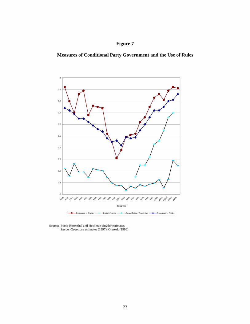
The results are visually evident in Figure 7. We report there the R2 measure from the

Poole and the Snyder estimates, since they are the most comparable between the two sets of

estimates and since they are neither the most nor least variable measure of conditional party

government. Of course, the restrictive rule measure is only available for a brief period, but it is

clear that it climbs dramatically and in line with increasing conditionality. The relationship with

the Snyder-Groselcose, party pressure measure is less visually apparent. Still, it is correlated

strongly with the conditional party government measures (e.g., r = .51 with Poole and .60 with

Snyder R2, with correlations with the other measures similar, if often slighter smaller). These

results support the theory of conditional party government. Precisely when the condition is

increasingly well satisfied, the majority party (at least) uses its powers to achieve what are now

increasingly evident collective aims among its members.

23

Figure 7

Measures of Conditional Party Government and the Use of Rules

Source: Poole-Rosenthal and Heckman-Snyder estimates, Snyder-Grosclose estimates (1997), Olesezk (1996)

0

0.1

0.2

0.3

0.4

0.5

0.6

0.7

0.8

0.9

1

8

0th

81st

82nd

83r

d

84th

8

5th

8

6th

87th

8

8th

8

9th

9

0th

91st

92n

d

9

3rd

9

4th

9

5th

9

6th

9

7th

9

8th

9

9th

1

00th

1

01st

1

02nd

1

03rd

1

04th

Congress

R-squared -- Snyder Party Influence Closed Rules - Proportion R-squared -- Poole

24

Discussion and Conclusions

In this paper, we have extended and more sharply defined the concept of conditional

party government. In particular, we have motivated the theory more clearly. Earlier (1997), we

demonstrated that, in a unidimensional policy space, there was at least the possibility (and, at

least given that the space was unidimensional, the possibility was realized under seemingly

plausible, perhaps even common conditions) of a collective action problem that the party could

solve. That is, every member of the majority party could be made better off by acting

collectively than by simply voting their preferences. That result did not demonstrate that the

party would solve the collective action problem, but indicated under what seemed to be the least

likely circumstances (i.e., unidimensionality) for parties to be “strong,” that they could do so.

Here, we extended that theoretical possibility result. We examined a two-dimensional

policy space, beginning with no commonality of preferences within the parties and with the

status quo already located centrally. We then demonstrated that the majority party could move

policy toward outcomes that its members preferred by a combination of preferences and

structure. As we might expect, when there was no commonality of preferences, it took a great

deal of structure to effect such a move – the majority party not only had more votes, but control

of the agenda (presumably through the committee system) and restrictions on amendments (i.e., a

strict germaneness rule). As the condition was increasingly satisfied, however, the ability of the

majority party to achieve outcomes preferable to its members over the policy center required less

structure and resources (e.g., only agenda control, plus the power of numbers and homogeniety

of preferences). As the theory of conditional party government predicts, the majority party was

25

not invulnerable based solely on relatively homogenous preferences. Finally, this example

allowed us to demonstrate that the condition could be increasingly well satisfied in two ways.

One is the election of Members with ideal point distributions that increasingly reflect the

condition – presumably the consequence of the changing nature of southern congressional

elections, for example (see Rohde, 1991). The second way is increasing saliency of the

dimensions that define partisan cleavages, relative to those that divide (at least) the majority

party. This second way sharpens the point that the distribution of policy preferences of Members

within the Congress is a consequence of elections, and that elections are also partisan. Thus, the

condition may be increasingly well satisfied either by having constituencies elect partisans who

hold similar preferences as their peers from elsewhere in the nation, or by having elections that

raise the salience of party cleavages, without necessarily imposing uniformity of position on

those dimensions. We return to this point below.

We next examined the Poole and Snyder estimates of ideal points for the Members of the

House over the 25 post-World War II Congresses. We examined four summary measures of

these distributions (across the primary dimension in both data sets) that tap aspects of the

condition in conditional party government. These aspects are how far apart are the typical

Democrat and Republican, how much variation is there in the ideal points of members of the

majority party, in comparison to the whole House, how much overlap is there of estimated ideal

points of Democrats and Republicans, and how strongly is party affiliation related to position on

the primary dimension. We then found that there was systematic variation over time in the

degree to which these aspects of the condition were satisfied in the post-War years. Starting at a

relatively high degree of satisfaction in the 1940s, these measures declined during the late 1960s

26

and early 1970s, only to climb again in the 1980s, reaching high points in the 100th through 104th

Congresses. While there is no absolute measure of the condition, the range of variation in the R2

measures and the comparison of the actual distribution of ideal point estimates for Congresses at

low and high degrees of satisfaction indicate that the variation is genuine and substantial.

The two sets of ideal point estimates do not yield identical results. Nonetheless, the two

yield similar patterns of change over time, thus reinforcing the basic conclusion – the condition

in conditional party government has been well and poorly satisfied, at least in the Poole and

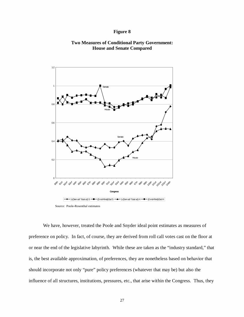
Snyder estimates, over the last fifty years. In Figure 8 we compare two measures of the

condition in House and Senate using the Poole estimates. We would not expect that the House

and Senate would be identical. Nonetheless, the variation over time is broadly similar. Both

House and Senate, by these measures, had relatively unified parties in the 1940s with substantial

decline in the late 1960s (perhaps less so in the Senate than in the House) and with a substantial

resurgence in the last decade. Indeed, it appears that the Senate may satisfy the condition even

more strongly than in the House in the 1990s. This finding reinforces our belief, as we will

discuss in more detail shortly, that electoral forces are partisan and that, therefore, the

preferences Members bring with them to the Congress are already shaped by partisan

institutions, even if those are partisan electoral institutions. It also supports our arguments that

we must systematically evaluate the agenda facing the Congress. For example, one reason that

Democrats were divided in the 1960s and 1970s was the salience of – and relatively frequent

voting on the floor on – civil rights.

27

Figure 8

Two Measures of Conditional Party Government:House and Senate Compared

Source: Poole-Rosenthal estimates

We have, however, treated the Poole and Snyder ideal point estimates as measures of

preference on policy. In fact, of course, they are derived from roll call votes cast on the floor at

or near the end of the legislative labyrinth. While these are taken as the “industry standard,” that

is, the best available approximation, of preferences, they are nonetheless based on behavior that

should incorporate not only “pure” policy preferences (whatever that may be) but also the

influence of all structures, institutions, pressures, etc., that arise within the Congress. Thus, they

0

0.2

0.4

0.6

0.8

1

1.2

8

0th

8

1st

82nd

83rd

8

4th

8

5th

8

6th

8

7th

8

8th

8

9th

90th

91st

92nd

9

3rd

9

4th

9

5th

9

6th

9

7th

9

8th

9

9th

10

0th

10

1st

1

02nd

1

03rd

10

4th

Congress

1-(Dem sd/ Total sd) S (D md-Rmd)/2sd S 1-(Dem sd/ Total sd) H (D md-Rmd)/2sd H

Senate

House

Senate

House

28

incorporate any influence of party, committee, lobbyist, presidential influence, etc. In our case,

we are particularly concerned with party and, indeed, have as a central part of our theoretical

claims the hypothesis that preference and intra-legislative party powers should be closely related.

We were able to assess systematically two indicators of intra-chamber rules and powers, and we

found them clearly and strongly related to the measures of conditional party government.

The finding that the use of rules and party organizational resources is positively

correlated with the measures has two important implications. Methodologically, it supports our

understanding of Krehbiel’s basic claim (1998) about the use of party or other roll call voting

measures. They are not “pure” measures of party strength – or of preferences. Rather they are

mixtures of all the forces that shape roll call voting on the floor of the Congress. Theoretically,

the correlation between the use of party-controlled resources within the House and both the

Poole and Snyder estimates that are based on roll call voting behavior is strong evidence in favor

of the theory of conditional party government. The theory predicts that the majority party will

want, collectively, to empower their party and use those resources precisely when their

preferences yield high degree of satisfaction of the condition.12

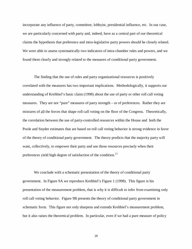
We conclude with a schematic presentation of the theory of conditional party

government. In Figure 9A we reproduce Krehbiel’s Figure 1 (1998). This figure is his

presentation of the measurement problem, that is why it is difficult to infer from examining only

roll call voting behavior. Figure 9B presents the theory of conditional party government in

schematic form. This figure not only sharpens and extends Krehbiel’s measurement problem,

but it also raises the theoretical problem. In particular, even if we had a pure measure of policy

29

preferences, as well as of rules and behavior, the measurement model would still be under-

identified. The connection between the electoral and legislative institutions of the party must

also be incorporated, both in statistical and in substantive-theoretical terms. Policy preferences

are not simply exogenous forces, but rather are the product of party and constituency (inter alia).

In the terms of the theory of conditional party government, the degree of satisfaction of the

condition is due, at least in part, to the effect of the party-in-elections. Thus, it is no mere

coincidence that, with a relative high degree of satisfaction of the condition, partisan Members of

Congress empower intra-legislative party organizations. Rather, the party-in-government is

strengthened, at least in part, because of the impact of the party-in-elections.

Figure 9Schematic Representation of Conditional Party Government

9A: Krehbiel’s Measurement Problem (1998, Figure 1)

Measurement model

Consequences

Not Observable Primary model (e.g., of parties)

9B: Conditional Party Government

Preferences Behavior

Party-in-Elections Party-in-government

Preferences Behavior Policy Outcomes

30

Bibliography

Aldrich, John H. (1995) Why Parties? The Origin and Transformation of Party Politics in America (Chicago, Ill.: University of Chicago Press).

______________ (1994) “A Model of a Legislature with Two Parties and a Committee System,”Legislative Studies Quarterly, 13 3:313-339.

Aldrich, John H., and David W. Rohde (1996a) “A Tale of Two Speakers: A Comparison ofPolicy Making in the 100th and 104th Congresses,” Paper delivered at the Annual Meetingof the American Political Science Association.

______________ (1996b) “The Republican Revolution and the House AppropriationsCommittee,” Paper delivered at the Annual Meeting of the Southern Political ScienceAssociation.

______________ (1997) “”Balance of Power: Republican Party Leadership and the CommitteeSystem in the 104th House,” Paper delivered at the Annual Meeting of the MidwestPolitical Science Association.

______________ (1997-98) “The Transition to Republican Rule in the House: Implications forTheories of Congressional Politics,” Political Science Quarterly, 112 4:541-567.

Carmines, Edward G., and James A. Stimson (1989) Issue Evolution: Race and theTransformation of American Politics (Princeton, N.J.: Princeton University Press).

Heckman, James J., and James M. Snyder, Jr. (1997) “Linear Probability Models of the Demandfor Attributes with an Empirical Application to Estimating the Preferences ofLegislators,” RAND Journal of Economics 28: S142-S189.

Krehbiel, Keith (1998) “Party Voting in a Nonpartisan Legislature,” Paper delivered at theAnnual Meeting of the Public Choice Society.

Oleszek, Walter J. (1996) Congressional Procedures and the Policy Process, 4th ed. (Washington,D.C.: CQ Press).

Poole, Keith T., and Howard Rosenthal (1985) “A Spatial Model for Legislative Roll CallAnalysis,” American Journal of Political Science, 29 2:357-84.

______________ (1997) Congress: A Political-Economic History of Roll Call Voting (NewYork: Oxford University Press).

Rohde, David W. (1991) Parties and Leaders in the Postreform House (Chicago, Ill.: Universityof Chicago Press).

31

Shesple, Kenneth A. (1989) “The Changing Textbook Congress,” in Can the GovernmentGovern?, ed. John Chubb and Paul Peterson (Washington, D.C.: Brookings Institution),pp. 238-66.

Snyder, James M. Jr., and Tim Groseclose (1997) “Party Pressure in Congressional Roll-CallVoting,” unpublished paper, MIT.

32

Endnotes

1 This is true even for the most moderate members of the majority party, and therefore those most vulnerable to theappeals from the minority to support policies closer to the median of the whole House. Essentially, the moreextreme partisans divert the resources granted the party under the conditional party government hypothesisdisproportionately toward their more moderate peers.

2 We would like to thank Keith Krehbiel for proposing the example in Figure 1. While we illustrate the logic in two-dimensions, there seems to be nothing special about two dimensions, and so we presume it is effectively an n-dimensional example.

3 Technically, the status quo is at the centroid of the ideal points in the policy space. We also assume that xs is thereversion point.

4 A third power, for example the ability to demand that any amendment be germane, if by that we mean that anyamendment can only change proposals in the dimensions the proposals themselves seek to change the status quo, issufficient. With a germaness rule, amendments are limited. A common spatial interpretation is that onlyamendments that change along the dimension or dimensions raised by the bill are germane. In this case, thedimension could be the line passing through xs and b. That is, the dimension is the dimension of party cleavage. Ifso, amendment a is out of order, and there is only a very small region in which successful amendments can beproposed. Indeed, if an amendment has to be literally on the line between xs and b, then d1 has no amendment thatmakes him or her better off and is also feasible.

5 More accurately, there is nothing in the petal of the win set of xs that includes d1 as part of its supporting majorityand that overlaps with the win set of b.

6 That is, if all Members have quadratic-based utility, and the only thing that changes from Figure 1 is an alterationof the quadratic base for determining the metric of distance, changing from the simple to the weighted Euclideannorm of distance, then there is a transformation of the norm back from weighted to simple Euclidean distance thatyields the distribution of ideal points as in Figure 3.

7 Nothing limits the argument to the House, of course (see below for a glimpse at Senate data).

8 We got the Poole-Rosenthal data off their web site. Jim Snyder provided us with the Heckman-Snyder estimatesand other data reported below. We are grateful to all of these scholars.

9 Party is strongly related to the first Poole dimension, but consistently if considerably less strongly related to theirsecond dimension. Party is related strongly to the first dimension in Snyder’s estimates, and essentially unrelated toany other dimension. We report the strength of these relationships to the two first dimensions as one of our fourmeasures of conditional party government, below.

10 We weight these by dividing by two times the standard deviation of the distribution of all ideal points in thatCongress, as a “standardized” measure, to facilitate comparison across Congresses and between measures. We usetwo times the standard deviation for scaling purposes (and, of course, corresponding to a range that, if done at thefloor median, would effectively encompass about two-thirds of all Members’ ideal points).

11 We use the Democratic party because it was the majority party for such a high proportion of these 25 Congresses.Switching to the Republican party when it formed the majority would include the unnecessary complication ofdifferences between the two parties (had we done so, it would have strengthened our assessments, so this was themore conservative choice). We do lose from this measure how very tight the distribution of ideal points of theRepublicans was in the 104th (less than half the most cohesive Democratic value for any Congress, and under three-quarters the magnitude of the next most cohesive Republican distribution [the 103rd]).

33

12 Put in slightly different terms, the methodological problem is that we observe behavior and assume that it is afunction of both preferences and institutions. By at least partially measuring institutional forces, we have taken onesignificant step towards identifying a still-unidentified equation (as implied in Figure 9).