Embed Size (px)
Citation preview
Measuring and modelling air mass flow rate in the injection stretchblow moulding process
Salomeia Y Menary G H Armstrong C G Nixon J amp Yan S (2016) Measuring and modelling air massflow rate in the injection stretch blow moulding process International Journal of Material Forming 9(4) 531-545DOI 101007s12289-015-1240-0
Published inInternational Journal of Material Forming
Document VersionPeer reviewed version
Queens University Belfast - Research PortalLink to publication record in Queens University Belfast Research Portal
Publisher rightsCopyright 2015 SpringerThe final publication is available at Springer via httpdxdoiorg101007s12289-015-1240-0rdquo
General rightsCopyright for the publications made accessible via the Queens University Belfast Research Portal is retained by the author(s) and or othercopyright owners and it is a condition of accessing these publications that users recognise and abide by the legal requirements associatedwith these rights
Take down policyThe Research Portal is Queens institutional repository that provides access to Queens research output Every effort has been made toensure that content in the Research Portal does not infringe any persons rights or applicable UK laws If you discover content in theResearch Portal that you believe breaches copyright or violates any law please contact openaccessqubacuk
Download date10 May 2018
1
Measuring and Modelling Air Mass Flow Rate in the Injection Stretch Blow Moulding Process
Y Salomeia1 G H Menary2 C G Armstrong2 J Nixon2 S Yan2
1 Blow Moulding Technologies 125 Stranmillis Road BT9 5AH Belfast Northern Ireland UK
yannisbmt-nicom
2 School of Mechanical and Aerospace Engineering Queenrsquos University of Belfast BT9 5AH
Belfast Northern Ireland UK
Contact Information for Corresponding Author
James Nixon
Queens University Belfast
School of Mechanical amp Aerospace Engineering
Ashby Building
Stranmillis Road
Belfast BT9 5AH
Northern Ireland
Tel +44 (0)28 9097 5523
Email jnixon05qubacuk
2
Abstract
The injection stretch blow moulding process involves the inflation and stretching of a hot preform
into a mould to form bottles A critical process variable and an essential input for process
simulations is the rate of pressure increase within the preform during forming which is regulated
by an air flow restrictor valve The paper describes a set of experiments for measuring the air flow
rate within an industrial ISBM machine and the subsequent modelling of it with the FEA package
AbaqusABAQUS Two rigid containers were inserted into a Sidel SBO1 blow moulding machine
and subjected to different supply pressures and air flow restrictor settings The pressure and air
temperature were recorded for each experiment enabling the mass flow rate of air to be determined
along with an important machine characteristic known as the lsquodead volumersquo The experimental
setup was simulated within the commercial FEA package AbaqusABAQUSExplicit using a
combination of structural fluid and fluid link elements that idealize the air flowing through an
orifice behaving as an ideal gas under isothermal conditions Results between experiment and
simulation are compared and show a good correlation
Keywords Stretch blow moulding simulation
3
10 Introduction
Injection Stretch Blow Moulding (ISBM) is the widely used process to manufacture Polyethylene
terephthalate (PET) bottles for the beverage and consumer goods industry With the ever growing
cost of raw materials and rapidly increasing competition PET bottle manufacturers have been
trying to push their limits to reduce the weight of the bottle without compromising the in service
performance and aesthetics of the bottle
The existing industrial state of the art in injection stretch blow moulding involves trial and error
approaches on a single cavity ISBM machine to determine appropriate machine settings for
industrial production Depending on the bottle and performpreform design this can take several
days to complete Most of the research over the last 20 years has focused on developing numerical
simulations to overcome this empirical approach and replace it with a more scientific method
whereby one can predict the process conditions and their effect on material thickness distribution
and material properties in advance
Chevalier et al has focused on modelling how PET behaves during processing and how processing
influences microstructure and macroscopic material properties [12] An aspect of their work has
focused on developing a blow moulding simulation based on the Constrained Natural Elements
Method (C-NEM) which has the advantage of not requiring any re-meshing even when the
elements are subjected to high strains [3] The simulation is still at an early stage of development
and no correlation between simulation and experiment is available Billon et al [4] has focused
on understanding how PET behaves during stretch blow moulding The microstructure of formed
bottles and lsquofree blownrsquo bottles have been analysed showing how the crystallinity and orientation
develops during stretch blow moulding and a numerical model of PET has been developed to
capture these features based on an Edwards Vilgis hyperelastic model Hopmann et al [5] have
4
developed an integrated blow moulding simulation approach where 3 simulations are integrated
together to model the complete history of the performpreform The 1st stage simulates the preform
during the heating phase which predicts a temperature profile of the preform This temperature
profile is subsequently used in a blow moulding simulation which predicts wall thickness and
mechanical properties These predictions are then fed into in-service performance simulations for
top load and shelf life Results for all stages correlate well with experiment although the results
are only presented for one test case and no information is provided on the validity of the
temperature predictions The work by Erichiqu et al [6] identified the need for modelling inflation
processes by using a fluid flow approach when considering inflation of a thin membrane however
their focus was on the mathematical implementation of this within FEA code rather than
measurement and validation
Bordival et al [7] developed an IR heating and ISBM simulation They coupled the ISBM
simulation to an optimization algorithm with the aim of predicting optimum preform temperature
profile that gave the most uniform wall thickness The IBSM simulation used a fluid structure
type approach within the commercial FEA package ABAQUS to calculate the air pressure
Corresponding experiments were performed on a simple prototype rig which could heat the
preform and then blow it into a simple mould without a stretch-rod The rig was able to measure
the pressure inside the preform whilst the mass flow rate was measured using a hot wire sensor
The sensor indicated that the mass flow was non-linear rising exponentially to a peak before
decaying gradually to zero It is not mentioned about the response time of the sensor and its
possible effect on the measurements and there are no details of the pneumatic circuit on the test
rig used It is important to note however that the timescale of inflation on this simple rig (4 sec)
is not comparable with that observed on an industrial ISBM machine where the bottle is typically
5
inflated in under 300ms [8] The difference in timescales suggests that the sensor may be
unsuitable for use on an industrial blow moulding machine as it is unlikely to be able to cope with
the transient flows experienced The ISBM simulation also incorporates heat transfer between the
mould and the preform and experimental data is presented for the heat transfer coefficient The
simulation had reasonable predictions for pressure evolution although the aggressive pressure drop
due to the large volume increase rate during bubble formation was predicted to be too fast ie the
bubble initiated too quickly in the simulation The thickness distribution of the formed bottle was
predicted with a 15 error An example of the potential power of ISBM simulation is shown by
coupling it to an optimization algorithm with the objective to produce a bottle with a uniform wall
thickness by modifying the preform temperature Schmidt et al [9] incorporated instrumentation
on a stretch blow moulding machine and noted that the pressure in the preform was substantially
different to that of the line pressure They propose a coupled model for the thermodynamics of
the air and for the thermo mechanical inflation of the preform They highlight the importance of
measuring the flow rate to accurately capture the pressure in the preform and suggest an
experiment involving pressurizing of a rigid volume This methodology is explored in this paper
Mir et al [10] also highlighted the fact that the pressure inside the preform is not constant and the
need to impose a mass flow rate of air rather than a directly applied pressure to accurately model
this They use a thermodynamic energy balance approach to calculate the flow rate based on the
energy supplied from the air compressor This is a reasonable first approximation but it is important
to note that there are no validation measurements and that the process is more complex than this
idealization eg typically the machine operator when optimizing their process tweaks a flow
control valve as the air enters the preform thus altering the flow rate Menary et al [11] in
collaboration with Billon conducted free-blow trials on an instrumented prototype rig Simulations
6
of the free-blow trials were developed and compared with the videos and the measured process
variables of pressure stretch rod force and local stretch ratio on the preform Two approaches
were taken for the simulation (i) the pressure was applied directly and measured (ii) a uniform
mass flow rate was applied to the preform that was calculated based on the volume evolution of
the preform and pressure inside it The results highlighted that the mass flow rate approach was
more realistic with excellent correlation between experiment and simulation In order to develop
reliable validated modelling instrumentation of the process is vital to ensure accurate and reliable
input of processing conditions into the simulation and for validating the outputs from the
simulation Recent work by the authors [812] has involved building a wireless data acquisition
system for measuring pressure inside the preform stretch rod force stretch rod displacement and
air temperature inside the preform This device is distinctive in that it is portable and can be
mounted on industrial ISBM machines In addition sensors have been incorporated inside a mould
to measure the moment of contact when the preform touches the mould surface and a separate
patented rig has been developed for measuring the inner and outer surface temperatures of the
preform These devices have enabled exact quantification of the process variables that are needed
as inputs to the ISBM simulation The challenge remains however to accurately quantify the flow
rate of air in an ISBM machine and to accurately represent it within an ISBM simulation The work
in this paper will use this instrumentation system to measure the pressure and temperature within
the preform and hence enable the mass flow rate to be calculated
It is clear from the reviewing the literature that there is a need to measure and model the air flow
within an ISBM machine in order to accurately represent the critical process variable of pressure
within an ISBM process simulation In this paper we perform practical experiments to measure the
7
mass flow rate and setup a corresponding model of the thermodynamic process within the
commercial finite element package ABAQUS
20ExperimentalSetup
All experiments were performed at Logoplaste Technologies (Cascais Portugal) In this case the
blow moulding machine used was a single mould automatic SBO1 stretch blow moulding machine
from Sidelcopy Company A simplified schematic diagram of the ISBM pneumatic system is shown
in Fig 1
The ISBM machine has a large buffer tank that stores air at 35MPa gauge pressure Subsequently
two lines for the pre-blow and final blow stages run from this tank For the pre-blow the pressure
is regulated down to a pressure in the range of 06 to 11 MPa gauge pressure The two lines are
fed to a complex valve block that commutes between pre-blow final-blow and exhaust For
simplicity in Fig 1 only the shut off valve corresponding to the pre-blow stage is represented In
addition upstream of the shut off valve a flow control valve is mounted to limit the maximum rate
at which the air enters the cavity The flow control valve used in this work has a scale of 12 units
however beyond index 6 in this system it behaves as a fully opened valve How an index on the
valve corresponds to flow resistance in a given set of units is not known
During the pre-blow stage the preform expands rapidly requiring a large mass of air For this reason
the pre-blow supply pipe between the pressure regulator and valve block is typically large in
diameter and in this case equates to a volume around 6 times the volume of the final bottle This
arrangement behaves as a buffer and prevents a large drop in the pressure upstream of the valve
block
8
The network of pipes typically found in industry connecting the compression stations and the
ISBM machine buffer are vast and heat gained during compressing is lost to the environment It is
therefore reasonable to assume that the air entering the system is at room temperature
Following the valve block the air flows through complex geometries such as pipes elbows sudden
changes of section ending with a flow straightener before it reaches the preform Pressure drops
are expected for such a pneumatic circuit however in this work they will not be considered
The main attention is directed towards the flow control valve It is typically used to finely adjust
the process and it is the scope of this work to understand its effect Such a restricting device causes
significant pressure drop in the fluid In the presented case air can be considered both an ideal and
compressible gas For such a gas the flow speed through a small cross section such as the flow
restrictor reaches a limit when the absolute pressure ratio between the inlet and outlet is 0528 It
is said that the flow is choked when the following condition is met
(1)
Where is the pressure measured inside the bottle and is the supply pressure measured
in the line
The mass flow rate through the restriction is
(2)
Where is the restrictor area ρ is the density of the fluid at the restriction which is assumed to be
constant as we assume constant inlet pressure and is the fluid velocity at the restriction
For downstream pressures smaller than 0528 Pline the mass flow is only influenced by the fluid
conditions upstream of the nozzle In this sense if the pressure and temperature of air in the
9
buffer tank remain constant the mass flow also remains constant as long as the choked condition
is met due to velocity limitations Eventually the downstream pressure will rise above 0528Pline
as the volume of the bottle fills with air and the pressure increases Beyond this condition the
increase in pressure in the cavity reduces the mass flow rate through the nozzle
In order to characterize the air mass flow a series of experiments summarized in Table 1 were
carried out involving charging two known fixed volumes These volumes are essentially a rigid
preform ie a preform at room temperature and a previously fully formed bottle constrained in a
mould Two levels of pressure and four settings of the flow restrictor over the range of interest
were selected resulting in 16 measurements
21 Rigid Volume Pressurisation
Along with the pressure measurement the temperature of the air within the cavity was also
measured via a fine wire thermocouple of 0075mm diameter embedded in the stretch rod Fig 2
and Fig 3 shows the pressure and temperature vs time for preform charging using a supply
pressure of 07MPa respectively whilst Fig 4 and Fig 5 shows the pressure and temperature vs
time for bottle charging using a supply pressure of 07MPa respectively Fig 6 and Fig 7 shows
the pressure and temperature vs time for preform charging using a supply pressure of 09MPa
respectively whilst Fig 8 and 9 shows the pressure and temperature vs time for bottle charging
respectively using a supply pressure of 09MPa respectively
Once the shut off valve is opened the pressure increases until equilibrium with the pressure in the
supply line is reached Yet the pressure plateau reached is less than the nominal pressure The
10
inaccuracy comes from the analogue pressure gauge fitted on the machine which is subject to
human error when set Nevertheless this systematic error does not affect the measurements as
great care was taken to be consistent in the adjustment of the pressure regulator
The high index experiments reveal two characteristics of the pressure history At the beginning the
pressure has a gradual rise This could be explained by inertia of the thermodynamic system or by
a hysteresis of the pressure sensor The second characteristic of the pressure measurement is the
overshoot in pressure that appears with indexes greater than 3 on this particular flow restrictor
valve Such a simple experiment cannot reveal the precise reason for this phenomenon however
it is thought to be a due to shockwave over imposed on the real measurement This is not likely to
appear in the actual forming process as the preform will deform resulting in a reduction of pressure
It was observed that the air temperature inside the cold preformbottle rose during the experiment
Moreover the temperature differs for different levels of line pressure and especially with flow
index This increase in temperature is normal and is due to the conversion of flow energy of the
stream of air filling the chamber into internal energy and the compression of the air already found
in the chamber As expected the minimum temperature rise of ~5degC occurred for the low flow
valve setting during pressurization of the bottle at the 07MPa supply pressure whilst the maximum
temperature rise occurred for the high flow valve setting pressurizing the preform with a 09 MPa
supply pressure
In order to explain the difference for different charging rates analysis of what would be the
expected temperature rise is performed Referring back to Fig 1 the dotted line indicates the
control volume of interest This is an unsteady process since the conditions within the control
volume are changing over time However this can be analysed as a uniform-flow process assuming
11
that the state of the fluid remains constant at the inlet The case of an adiabatic vessel is considered
where the volume is equal to the value of the dead volume plus the volume of the rigid container
The calculation of the dead volume inferred here is explained in detail in the next section
Noting that the microscopic energies of flowing and non-flowing fluids are represented by
enthalpy h and internal energy u respectively the mass and energy balances for this uniform-flow
system can be expressed
Mass balance
∆ (3)
Where is the mass of air entering the system is the mass of air leaving the system
is the mass of air in the preformbottle at the end of the experiment and is initial mass of air in
the preformbottle
Since 0
(4)
Energy balance
∆ (5)
Where is the Energy put in to the system is the Energy leaving the system and ∆
is the change in Energy
Since 0
(6)
Which can be written as
12
(7)
Where is the temperature of air entering the system is the temperature of air in the
preformbottle at the end of the experiment and is the initial temperature of air in the
preformbottle is the specific heat capacity of air at constant pressure is the specific heat
capacity of air at constant volume
Combining equation 4 and 7
(8)
The initial and final masses are given by the equation of state
(9)
Where is the intial pressure in the preform is the final pressure in the preform V is the
volume of the preformbottle plus the dead volume and R is the gas constant
Substituting the gas constant of air R=287 Pa m3 kg K and the specific heats of air at the system
temperature cp air20oC=1004 Jkg K and cv air20oC=716 Jkg K and the boundary conditions
line pressure of 07 MPa inlet air at 20oC and volume V=670middot10-6m3 yields the temperature
T2asymp118oC for 07 MPa line pressure and asymp122oC for 09 MPa line pressure
These values indicate that if no heat is exchanged with the environment a significant increase in
temperature is expected The variation in temperature with the rate of charging is justified by the
variation in time necessary to fill the volume which allows more time for heat exchange with the
metallic components of the system
13
Due to difficulties encountered during mounting of the fine wire thermocouple only a 0075mm
thermocouple wire could be installed Some underestimation of the real temperature was expected
however the maximum value recorded is around 53oC which is well below the calculated value
In addition it should be noted that the plotted temperature values are interpolated values and in
reality the temperature acquisition rate was only 7Hz due to hardware restrictions In these
conditions there is likelihood for aliasing to occur as the temperature oscillation happens quicker
than the sampling rate resulting in measurements that may be potentially higher in magnitude being
missed Using a lumped capacitance method and treating the bead of the thermocouple as a sphere
equation 9 can be used to estimate the time constant of the thermocouple to detect a rise in air
temperature from 20degC to 100 degC to be approximately 008 seconds Considering the peak
temperature rise is recorded within 006 seconds it seems likely that the response time of the
thermocouple is affecting the results
(10)
Where ρ is the metallic bead density (8665 kgm3) D is the bead diameter (01875 ∙ 10 m c is
specific heat respectively of the bead (486 J kg ∙ Kfrasl ) and h is the convection coefficient which is
estimated to be 1600 ∙frasl from calculations based on a Nusselt number of 10 and a
conductivity of air of 3010-3 (WmK)
It can be concluded that the charging process in the given conditions is neither adiabatic nor
isothermal but is more a ldquoquasi-adiabaticrdquo process with a polytropic index γ in the range 1 to 14
depending on the charging rate
14
30Deadvolume
The summation of the individual volumes described in the previous section downstream of the
flow control valve is part of the thermodynamic system considered in this work and it is referred
to as lsquodead volumersquo as it remains unchanged An accurate value could not be found in the machine
documentation and the detailed technical drawings are confidential From visual inspection
however it was clear the volume is at least the same order of magnitude as the final volume of the
bottle hence some sort of calculation is needed to eliminate the inaccuracy in its value that could
introduce significant errors in subsequent calculations for the mass flow rate
The calculation is based on the experiment that involves charging of two containers of different
known volumes in the case closest to an isothermal process ie low supply pressure (07 MPa and
high restriction (index =1)
An assumption is made that the time scale of the experiments are considered slow to enable any
heat generated to be dissipated and therefore both processes are isothermal We also assume that
due to the small opening of the flow restrictor the mass flow at that control volume is considered
choked as long as the condition Pbottle lt 0528Pline is satisfied
Based on the equation of state and assuming isothermal conditions we define the rate of mass of
air at any point in time in the system to be
∙ (11)
Writing the mass flow for both cases
15
RT
VV
dt
dP
RT
V
dt
dPm pDAAA
preform
)(
RT
VV
dt
dP
RT
V
dt
dPm pDAAA
preform
)(
(12)
Where VA = Volume composed of the volume that remains unchanged over the experiments (dead
volume VD) plus the volume of a pre-form (Vp)
RT
VV
dt
dP
RT
V
dt
dPm bDBBB
bottle
)(
RT
VV
dt
dP
RT
V
dt
dPm bDBBB
bottle
)(
(13)
Where VB = Volume composed of dead volume plus the volume of a fully formed bottle (Vb)
The choked condition therefore implies
(14)
Rearranging equations 1011 and 12
∙ ∙ (15)
and can be found from the initial gradient in Fig 10 to be 037 MPasec and 019 MPasec
respectively whilst the volume of the preform and bottle were measured to be 215 ml and 675ml
respectively Substituting these values in to eq 15 yields a value of asymp670ml Since the dead
volume is of the order 30 times greater than the original preform volume it is obvious of the
need to incorporate it into any calculations
It was shown in Fig 3 5 7 and 9 that the recorded temperature history of the cavity air during
charging of the cold rigid preforms and bottles indicate that the process is neither isothermal nor
adiabatic Some heat is lost to the machine parts and in the actual forming process it can be
expected that heat will be gained from the hot preform However during the blowing process
work is done from the inflating preform and without accurate knowledge of the volume evolution
Field Code Changed
Field Code Changed
16
it cannot be estimated It therefore is more sensible to calculate the flow rate from the pressure
curves generated from charging of the rigid containers Assuming isothermal conditions the mass
flow rate in the initial choked phase can then be evaluated by eq 11 where frasl is the initial
slope of the pressure in the cavity and the volume V represents the volume downstream of the flow
restrictor composed of the dead volume and the preformbottle volume
Eq 11 or eq 16 both enable the flow rate to be estimated assuming choked conditions however it
can be expected that during the ISBM forming process that the condition of Pbottle lt 0528Pline will
not always be met Fig 11 shows how the mass flow rate changes with the ratio between line
pressure (Pline) and the pressure in the bottle (Pbottle)
By definition the flow in the choked region is constant up until a ratio of 0528 after which the
flow decays in a non-linear fashion towards zero when the pressure in the bottle equals the line
pressure This graph can be described mathematically by eq 16 and 17 where eq 16 describes
the flow in the choked region and the eq 17 describes the flow in the un-choked region [13]
fraslfrasl
(16)
frasl frasl
(17)
Where CD is the coefficient of discharge AT is the cross section of the nozzle R is ideal gas
constant γ is the specific heat ratio Pline is the absolute Air pressure in the supply line and Pbottle
is the absolute air pressure in the bottle
Formatted equationY Left
Formatted equationY Centered
17
The discharge coefficient and the cross section of the valve are not known however their product
can be calculated The implementation of these equations into AbaqusABAQUS will be discussed
in the following section
Using eq 11 and 16 a value for the product of coefficient of discharge and the cross section of the
nozzle ( ) can be determined which can be substituted into eq 17 to find the un-choked flow
behaviour for each of the 8 combinations of flow index and supply pressure (Fig 13)
40RigidPressurisationSimulation
The pressure during blowing is a function of the supply line flow control valve index the volume
of the preform and the ldquodead volumerdquo The simulation package AbaqusABAQUSExplicit used in
this work conveniently permits input of the fluid mass flow rate as a function of pressure difference
using the fluid exchange process The volume is then calculated based on the deformation of the
material caused by the accumulated pressure in each time step
The objective of this simulation was to validate the mass flow and dead volume calculations by
comparing the simulated internal pressure in the preformbottle with the experimental internal
pressure
For the rigid pressurization simulation an axisymmetric model representing the preformbottle
volume and the dead volume was created in AbaqusABAQUS shown in Fig 14 The symmetric
design of the preform along an axis can be utilized in building an axisymmetric model which
reduces the simulation time The entire model is encastred (held rigidly) so that the preformbottle
does not expand under pressure which replicates the rigid pressurization tests The shape or
properties of the preformbottle do not have any effect on the results as the model is completely
18
rigid A fluid exchange process was used for simulating the air flow seen in rigid pressurization
test by supplying it with mass flow as function of ∆P (Fig 15) where ∆P is the difference between
supply pressure and the preform internal pressure AbaqusABAQUS interpolates linearly between
the values specified The calculated dead volume was incorporated into simulation such that the
mass flow of air fills the dead volumepreform combination thereby replicating the real rigid
pressurization tests It is also possible for the dead volume to be represented by a single node with
an ldquoadded volumerdquo equal to a value of 670ml as measured experimentally
The fluid exchange process in the AbaqusABAQUSExplicit package requires the mass flow
value to be supplied as a function of ∆P The mass flow values as function of ∆P are different for
each experiment Fig 15 shows the mass flow values as function of ∆P for the rigid pressurization
experiment of a 675ml bottle at 7 bar pressure and n=1
41 Rigid Pressurization Simulation Results
From section 21 it can be recalled that flow characterization for the preform was carried out
assuming isothermal conditions For the rigid volume pressurization simulations the cavity
pressure output was compared to that obtained from the experimental analysis The preform and
bottle pressurization was compared for flow conditions 9 bar n=1 Fig 16 and for flow conditions
9 bar n=6 Fig 16
It can be seen in Fig 16 and 17 that the simulation result matches very closely with the experiment
The predicted linear pressure gradient matched extremely well to that of the experimental gradient
with an R2 value of 0999 for all rigid pressurization scenarios This highlighted the fact that the
flow calculation method and application to the simulation proved successful The transition from
choked flow to un-choked flow was also well predicted for the low flow condition ie the gradient
19
reduction to constant pressure This transition was predicted less successfully for the high flow
rate A large lsquospikersquo in pressure was evident for the high flow rate condition after the linear gradient
and before the pressure levelled out to the line pressure value As was discussed earlier this
speculated to be as a result of a shock wave This prediction is not achievable using the fluid
exchange options in AbaqusABAQUS and would require some form of computational fluid
dynamics (CFD) in order to accurately calculate the air flow into the cavity at the higher flow rates
It is also not of great importance as this situation is as a result of the characterization method and
is unlikely to occur in an actual stretch blow moulding process
50ImplicationstoISBMSimulation
As previously mentioned the air mass flow rate is calculated directly from the linear pressure
gradient for a given cavitydead volume ie the air mass flow rate varies relative to the volume in
order to return the correct pressure gradient The dead volume therefore has no direct effect on the
predicted cavity pressure results adjustment of the air mass flow rate will account for this
Critically however the acknowledged dead volume and correct air mass flow rate has a significant
effect on the cavity pressure during the deformation of the preform ie non-rigid pressurization
To demonstrate this a simulation has been setup of a previously performed free blow experiment
[15]
A full Design of Experiments was carried out at different preform temperatures while varying the
air flow rate and the pre-blow timing The experiments were carried out on a semi-automatic lab
scale machine produced by Vitalli and Son This machine has a dead volume of 85ml which was
calculated using the method described in sectionSection 30 The corresponding simulation was
20
then also constructed with the calculated air mass flow rate for both rigid pressurization and free-
blow scenarios
51 Free-blow Simulation Set-up
The free-blow simulation was constructed in the same manner as the rigid pressurization
simulation with the addition of a suitable sub-routine to represent the viscoelastic material
behaviour of PET at temperature above Tg The PET material used for the free-blow trail had a Tg
of approximately 79degC an IV value of 081dLg and a density of 133gcm3 The material model
was developed by Shiyong Yan [16] and applied to the ABAQUSExplicittrade FEA using a
VUMAT user sub-routine The model was primarily based on the established Buckley model [17
18] a constitutive model that utilised two parallel parts the bond stretching part and the
conformation part Fig 18 Each part of the constitutive model was represented by complex
equations that required a large amount of data to perform accurate curve fitting procedures The
material data used for the curve fitting procedure and as a result the material constants were
determined from extensive material testing using the QUB biaxial stretcher [19 20] and strain
history form the DIC analysis of the FSB trials The biaxial testing was performed on
76x76x05mm samples of PET cut from extruded sheet the same grade as the preform material
Yan then modified the model to take into account strain rate and deformation mode During
material testing the temperature strain rate and deformation mode were used as the parameters to
attain the appropriate stress-strain curves Table 2 displays the test parameters used to provide data
for the characterisation procedure
21
The material model was built to take into consideration axisymmetric simulations (SAX1 shell
elements) and full 3D simulations (S4R shell elements) Only SAX1 shell elements were used
however for the preform for all the simulations in this work
52 Effect of Dead-volume
The simulation of the rigid pressurization for the preform volume was initially performed using
two volumes for the air mass flow calculation the preform on its own and the preform attached
to the dead volume The calculated air mass flow rate for the low flow rate setting was 14gs for
preform only and 67gs for attached dead volume For the high flow rate trial the air mass flow
rate was calculated to be 87gs for preform only and 401gs for attached dead volume The air
mass flow rate reduces as the volume is reduced in order to reproduce the same pressure gradient
Fig 1819 indicates that as expected the rigid pressurization for the two volume scenarios is the
same both scenarios would appear to be correct
However taking the cavity pressure results from two trials and comparing them to the predicted
cavity pressure during free-blow analysis highlights the effect of neglecting the dead volume
These air mass flow rates with respective volumes were then applied to the free-blow simulation
and the cavity pressure for each scenario was then compared to the experimental data Fig 1920
and 2021
The delay in the pressure rise for the low flow setting was due to a deliberate pre-blow timing
delay The effect of not accounting for the dead volume clearly had an effect on the cavity pressure
results and to a further extent how the bottle deformed each flow rate trial significantly under-
predicted the cavity pressure Examining each dead volume blowing scenario compared to the
experimental results yields that the low flow set-up had an R2 value of 0861 with the dead volume
22
neglected and 0985 when the dead volume was attached The high flow set-up had an R2 value of
0031 and 093 for the two dead volume set-ups respectively It is important to remember that
during the initial phase as the pressure rises and contrary to the rigid pressurization trials the
stretch rod deforms the preform therefore increasing the cavity volume The change in cavity
volume with respect to the initial volume is greater for the scenario where no dead volume is
attached and therefore has a greater effect on the resultant output cavity pressure
Although the experimental and predicted pressure curves correlated successfully when the
appropriate dead volume was attached there was a certain amount of deviation as the free-blow
bottle deformed This was accounted for by the preform temperature profile used for the simulation
and the material model used to capture the viscoelastic behaviour of PET This can also be seen
when the bottle shape evolution is examined
53 Free-blow Analysis
The free-blow experiments were performed using the lab-scale ISBM instrument located at
Queenrsquos University Belfast employing a speckle patterned preform and theheated using a silicone
oil bath The deformation was captured using high-speed stereoscopic CCD cameras [R] Digital
image correlation analyses were then carried out to determine the strain levels on the deforming
surface The evolving bottle shape from the experiment was compared to that determined from the
Abaqus simulation Fig 21 along with the bottle shape at critical time points on the pressure
curveABAQUS simulation along with the cavity pressure and true strain from the outside surface
midpoint of the sidewall of the preform The predicted results were then compared to the
experimental values for low flow rate (Fig 22) and high flow rate (Fig 23) trials using the same
preform temperature of 100degC
23
The bottle shape comparison success deteriorates as the blowing process progresses from point A
to point E contrary to the pressure curve which appeared to correlate with greater accuracy This
highlights the fact that the mass flow rate and cavity pressure calculation is not governed by the
cavity shape but primarily the cavity volume
The low flow rate trial exhibits excellent cavity pressure comparison with an R2 value of 095 The
evolving bottle comparison however indicated that the bottle profile differed between the
simulation and the experiment the simulation appeared to expand faster than the experiment This
was confirmed examining the true strain results with an R2 value of 092 for both the hoop and
axial directions The final strain values also indicate that the experimental bottle shape was bias in
the axial direction ie slender bottle while the predicted bottle shape was bias in the hoop direction
ie fatter bottle The high flow rate trial comparison shows a less accurately predicted cavity
pressure than the low flow trial with an R2 value of 092 Comparing the evolving bottles of the
experiment and the simulation indicates that shape profile was predicted with high accuracy
emphasised by the surface strain results comparison of the strain results had R2 values of 099 and
096 in the hoop and the axial directions respectively The results highlight the fact that the mass
flow rate and cavity pressure calculation is not governed by the cavity shape but primarily the
cavity volume
The nature of the high flow rate preform expansion is primarily a form of biaxial deformation
although not purely equal biaxial the deformation occurs simultaneously in the hoop and axial
directions The construction of the material model using the biaxial stretching machine utilised
biaxial deformation therefore resulting in an accurately predicted high flow rate free-blow
simulation Contrary to this the low flow rate preform expansion takes the form of a sequential
type ie a linear axial stretch followed by a biaxial inflation The material characterisation
24
technique using the biaxial stretching machine was not able to replicate the sequential deformation
type for every foreseeable stretch scenario indeed only constant width and pure biaxial
deformation were captured The amount of initial linear stretch and therefore the onset of
orientation and eventual strain hardening [19-29] significantly affects the inflation of the preform
60Conclusions
An experimental methodology for determining the flow rate on an industrial injection stretch blow
moulding machine has been described The ideal gas law with the assumption of isothermal
conditions for the air has been used to calculate the flow rate Whilst the experimental
measurement of temperature indicates that this assumption is not ideal it has been demonstrated
that it is adequate for giving a realistic representation of the flow rate for an injection stretch blow
moulding process
The experiments have also highlighted a methodology for determining the ldquodead volumerdquo on a
blow moulding machine and the corresponding numerical simulations highlight the importance of
representing this volume in order to obtain accurate blow moulding simulations The data
generated has been used to setup a coupled fluid structure interaction problem in the commercial
finite element package AbaqusABAQUS assuming an ideal gas law for an incompressiblea
compressible fluid under isothermal conditions The simulations are able to replicate the rigid
charging experiments accurately except in the case where shock waves occur due to the high flow
The methodology developed has been applied to determine the flow characteristics of an additional
blow moulding machine which has the capability of performing free-blow experiments whilst
monitored via high speed camera The correlations between the model and the experimental data
25
for both evolving preform shape and the pressure vs time inside the preform validate the mass flow
measurements
26
Table 1 Summary of experiments used in charging fixed volumes
Flow index
(preform)
Flow index
(bottle)
Gauge pressure
(MPa)
07 1 2 4 6 1 2 4 6
09 1 2 4 6 1 2 4 6
Table 2 Summary of testing parameters for material characterisation
Temperature (degC) Strain Rate (s) Deformation Mode
90 1 Biaxial
95 2 Constant width
100 4
105 8
110 16
Formatted Font 16 pt
Formatted Centered
27
References
1 L Chevalier Y Marco Mech Mater 39 6 596 (2007)
2 Chevalier L Luo YM Monteiro E Menary GH Mech Mater 52 (2012)
3 B Cosson L Chevalier J Yvonnet Int J Mater Form 1 707 (2008)
4 Billon N Picard M Gorlier E Int J Mater Form DOI 101007s12289-013-1131-1
5 Hopmann C Michaeli W Rasche S 14th International Esaform conference on
Material Forming Belfast N Ireland (2011)
6 F Erichiqui A Bendana IJSPM 27 3 (2007)
7 M Bordival F M Schmidt Y Le Maoult V Velay Polym Eng Sci 49 4 783 (2009)
8 Y M Salomeia G H Menary C G Armstrong Adv Poly Tech 32 436 (2013)
9 F M Schmidt JF Agassant M Bellet Polym Eng Sci 38 9 1399 (1998)
10 H Mir F Thibault R Diraddo Polym Int 2011 2 173 (2011)
28
11 GH Menary CW Tan CG Armstrong Y Salomeia M Picard N Billon E Harkin-
Jones Polym Eng Sci 50 5 1047 (2010)
12 Y M Salomeia G H Menary C G Armstrong Adv Poly Tech 32 771 (2013)
13 J B Heywood Internal Combustion Engine Fundamentals McGraw-Hill New York
(1988)
14 M D Bughardt and J A Harbach ldquoEngineering Thermodynamicsrdquo Cornell Maritime
Press Centreville Maryland 4 ed (1993)
15 J Nixon S Yan G Menary Key Eng Mater 554-557 1729 (2013)
16 S Yan ldquoModelling the Constitutive Behaviour of Poly(ethylene terephthalate) for the
Stretch Blow Moulding Processrdquo PhD thesis Queenrsquos University Belfast (2013)
17 C P Buckley D P Jones Polymer 36 3301 (1995)
18 CP Buckley D P Jones Polymer 17 2403 (1996)
19 G H Menary C W Tan C G Armstrong Key Eng Mat 1117 504 (2012)
20 G H Menary C W Tan E M Harkin-Jones C G Armstrong P J Martin Polym Eng
Sci 52 671 (2011)
21 L Chevalier Y Marco Mech of Mat 39 596 (2007)
22 Y Marco L Chevalier M Chaouche Polymer 43 6569 (2002)
23 S Ahzi A Makradi R V Gregory D D Edie Mech of Mat 35 1139 (2003)
24 E Gorlier J M Haudin N Billon Polymer 42 9514 (2001)
25 CI Martins M Cakmak Polymer 48 2109 (2007)
26 E Deloye J-M Haudin N Billon Int J Mater Form 1 715 (2008)
27 N Billon M Picard E Golier Int J Mater Form 7 369 (2014)
29
28 A Mahendrasingam C Martin W Fuller D J Blundell R J Oldman J L Harvie D
H Mackerron C Riekel P Engstrom Polymer 40 5553 (1999)
29 A Mahendrasingam D J Blundell C Martin W Fuller D H MacKerron J L Harvie
R J Oldman C Riekel Polymer 41 7803 (2000)
15
Formatted Normal No bullets or numbering Adjust spacebetween Latin and Asian text Adjust space between Asian textand numbers
30
Figure Captions
Fig 1 Schematic diagram of the ISBM pneumatic system
Fig 2 Experimental measurement of pressure for preform charging with 07MPa supply pressure
Fig 3 Experimental measurement of temperature for preform charging with 07MPa supply
pressure
Fig 4 Experimental measurement of pressure for bottle charging with 07MPa supply pressure
Fig 5 Experimental measurement of temperature for bottle charging with 07MPa supply pressure
Fig 6 Experimental measurement of pressure for preform charging with 09MPa supply pressure
Fig 7 Experimental measurement of temperature for preform charging with 09MPa supply
pressure
Fig 8 Experimental measurement of pressure for bottle charging with 09MPa supply pressure
Fig 9 Experimental measurement of temperature for bottle charging with 09MPa supply pressure
Fig 10 Linear pressure gradient for preform and bottle pressurisation under flow conditions 7 bar
and n=1
Fig 11 Schematic of choked and un-choked flow
Fig 12 Maximum (choked) mass flow rate as a function of line pressure and flow index
Fig 13 Calculated un-choked mass flow rate of rigid pressurization tests as a function of pressure
ratio
Fig 14 Screen shot of 2D axisymmetric model used for the simulation of the rigid pressurisation
test
Fig 15 Mass flow as function of ∆P for the rigid pressurisation test of bottle at 7 bar and n=1
Fig 16 Comparison of predicted and experimental pressure for rigid pressurisation using flow
conditions at 9 bar and n=1 rigid preform and bottle
31
Fig 17 Comparison of predicted and experimental pressure for rigid pressurisation using flow
conditions at 9 bar and n=6 rigid preform and bottle
Fig 18Fig 18 Constitutive characteristic of the Buckley model
Fig 19 Rigid pressurisation of preform with and without dead volume attached low flow and high
flow rate
Fig 19 Experiential and predicted cavity pressure comparison for each dead volume scenario low
flow rate
Fig 20 Experiential and predicted cavity pressure comparison for each dead volume scenario low
flow rate
Fig 21 Experiential and predicted cavity pressure comparison for each dead volume scenario high
flow rate
Fig 2122 Evolving bottle shape for low flow rate trial with critical time points from pressure curve
and strain mapping experiment and simulation
Fig 23 Evolving bottle shape for high flow rate trial with critical time points from pressure curve
and strain mapping experiment and simulation
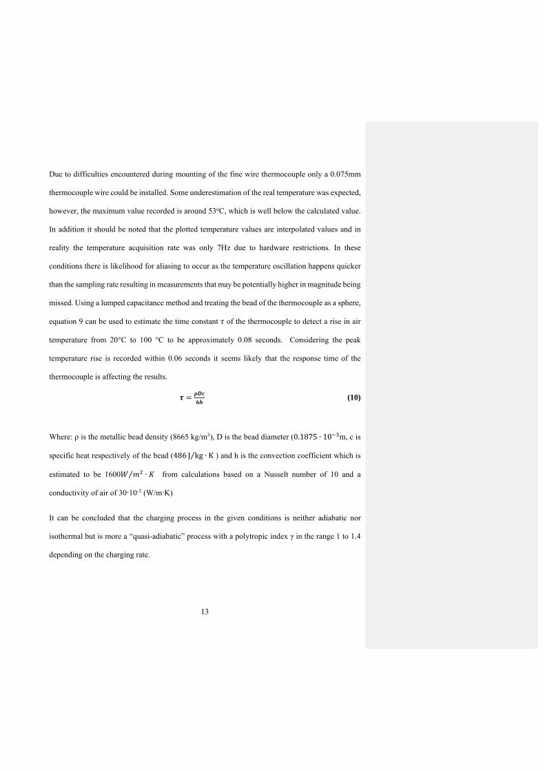
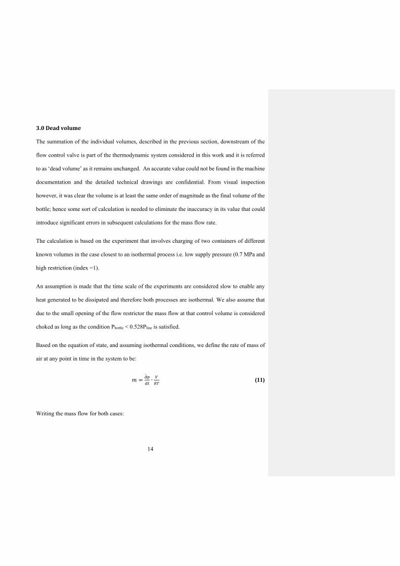
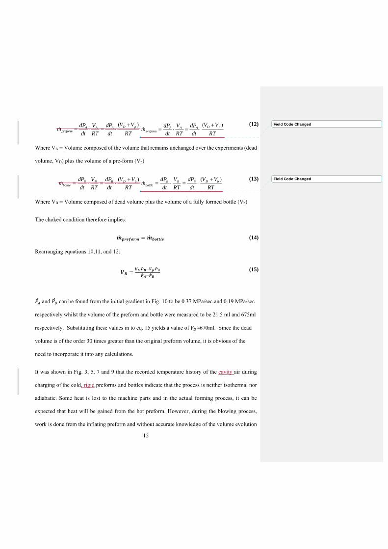
15
RT
VV
dt
dP
RT
V
dt
dPm pDAAA
preform
)(
RT
VV
dt
dP
RT
V
dt
dPm pDAAA
preform
)(
(12)
Where VA = Volume composed of the volume that remains unchanged over the experiments (dead
volume VD) plus the volume of a pre-form (Vp)
RT
VV
dt
dP
RT
V
dt
dPm bDBBB
bottle
)(
RT
VV
dt
dP
RT
V
dt
dPm bDBBB
bottle
)(
(13)
Where VB = Volume composed of dead volume plus the volume of a fully formed bottle (Vb)
The choked condition therefore implies
(14)
Rearranging equations 1011 and 12
∙ ∙ (15)
and can be found from the initial gradient in Fig 10 to be 037 MPasec and 019 MPasec
respectively whilst the volume of the preform and bottle were measured to be 215 ml and 675ml
respectively Substituting these values in to eq 15 yields a value of asymp670ml Since the dead
volume is of the order 30 times greater than the original preform volume it is obvious of the
need to incorporate it into any calculations
It was shown in Fig 3 5 7 and 9 that the recorded temperature history of the cavity air during
charging of the cold rigid preforms and bottles indicate that the process is neither isothermal nor
adiabatic Some heat is lost to the machine parts and in the actual forming process it can be
expected that heat will be gained from the hot preform However during the blowing process
work is done from the inflating preform and without accurate knowledge of the volume evolution
Field Code Changed
Field Code Changed
16
it cannot be estimated It therefore is more sensible to calculate the flow rate from the pressure
curves generated from charging of the rigid containers Assuming isothermal conditions the mass
flow rate in the initial choked phase can then be evaluated by eq 11 where frasl is the initial
slope of the pressure in the cavity and the volume V represents the volume downstream of the flow
restrictor composed of the dead volume and the preformbottle volume
Eq 11 or eq 16 both enable the flow rate to be estimated assuming choked conditions however it
can be expected that during the ISBM forming process that the condition of Pbottle lt 0528Pline will
not always be met Fig 11 shows how the mass flow rate changes with the ratio between line
pressure (Pline) and the pressure in the bottle (Pbottle)
By definition the flow in the choked region is constant up until a ratio of 0528 after which the
flow decays in a non-linear fashion towards zero when the pressure in the bottle equals the line
pressure This graph can be described mathematically by eq 16 and 17 where eq 16 describes
the flow in the choked region and the eq 17 describes the flow in the un-choked region [13]
fraslfrasl
(16)
frasl frasl
(17)
Where CD is the coefficient of discharge AT is the cross section of the nozzle R is ideal gas
constant γ is the specific heat ratio Pline is the absolute Air pressure in the supply line and Pbottle
is the absolute air pressure in the bottle
Formatted equationY Left
Formatted equationY Centered
17
The discharge coefficient and the cross section of the valve are not known however their product
can be calculated The implementation of these equations into AbaqusABAQUS will be discussed
in the following section
Using eq 11 and 16 a value for the product of coefficient of discharge and the cross section of the
nozzle ( ) can be determined which can be substituted into eq 17 to find the un-choked flow
behaviour for each of the 8 combinations of flow index and supply pressure (Fig 13)
40RigidPressurisationSimulation
The pressure during blowing is a function of the supply line flow control valve index the volume
of the preform and the ldquodead volumerdquo The simulation package AbaqusABAQUSExplicit used in
this work conveniently permits input of the fluid mass flow rate as a function of pressure difference
using the fluid exchange process The volume is then calculated based on the deformation of the
material caused by the accumulated pressure in each time step
The objective of this simulation was to validate the mass flow and dead volume calculations by
comparing the simulated internal pressure in the preformbottle with the experimental internal
pressure
For the rigid pressurization simulation an axisymmetric model representing the preformbottle
volume and the dead volume was created in AbaqusABAQUS shown in Fig 14 The symmetric
design of the preform along an axis can be utilized in building an axisymmetric model which
reduces the simulation time The entire model is encastred (held rigidly) so that the preformbottle
does not expand under pressure which replicates the rigid pressurization tests The shape or
properties of the preformbottle do not have any effect on the results as the model is completely
18
rigid A fluid exchange process was used for simulating the air flow seen in rigid pressurization
test by supplying it with mass flow as function of ∆P (Fig 15) where ∆P is the difference between
supply pressure and the preform internal pressure AbaqusABAQUS interpolates linearly between
the values specified The calculated dead volume was incorporated into simulation such that the
mass flow of air fills the dead volumepreform combination thereby replicating the real rigid
pressurization tests It is also possible for the dead volume to be represented by a single node with
an ldquoadded volumerdquo equal to a value of 670ml as measured experimentally
The fluid exchange process in the AbaqusABAQUSExplicit package requires the mass flow
value to be supplied as a function of ∆P The mass flow values as function of ∆P are different for
each experiment Fig 15 shows the mass flow values as function of ∆P for the rigid pressurization
experiment of a 675ml bottle at 7 bar pressure and n=1
41 Rigid Pressurization Simulation Results
From section 21 it can be recalled that flow characterization for the preform was carried out
assuming isothermal conditions For the rigid volume pressurization simulations the cavity
pressure output was compared to that obtained from the experimental analysis The preform and
bottle pressurization was compared for flow conditions 9 bar n=1 Fig 16 and for flow conditions
9 bar n=6 Fig 16
It can be seen in Fig 16 and 17 that the simulation result matches very closely with the experiment
The predicted linear pressure gradient matched extremely well to that of the experimental gradient
with an R2 value of 0999 for all rigid pressurization scenarios This highlighted the fact that the
flow calculation method and application to the simulation proved successful The transition from
choked flow to un-choked flow was also well predicted for the low flow condition ie the gradient
19
reduction to constant pressure This transition was predicted less successfully for the high flow
rate A large lsquospikersquo in pressure was evident for the high flow rate condition after the linear gradient
and before the pressure levelled out to the line pressure value As was discussed earlier this
speculated to be as a result of a shock wave This prediction is not achievable using the fluid
exchange options in AbaqusABAQUS and would require some form of computational fluid
dynamics (CFD) in order to accurately calculate the air flow into the cavity at the higher flow rates
It is also not of great importance as this situation is as a result of the characterization method and
is unlikely to occur in an actual stretch blow moulding process
50ImplicationstoISBMSimulation
As previously mentioned the air mass flow rate is calculated directly from the linear pressure
gradient for a given cavitydead volume ie the air mass flow rate varies relative to the volume in
order to return the correct pressure gradient The dead volume therefore has no direct effect on the
predicted cavity pressure results adjustment of the air mass flow rate will account for this
Critically however the acknowledged dead volume and correct air mass flow rate has a significant
effect on the cavity pressure during the deformation of the preform ie non-rigid pressurization
To demonstrate this a simulation has been setup of a previously performed free blow experiment
[15]
A full Design of Experiments was carried out at different preform temperatures while varying the
air flow rate and the pre-blow timing The experiments were carried out on a semi-automatic lab
scale machine produced by Vitalli and Son This machine has a dead volume of 85ml which was
calculated using the method described in sectionSection 30 The corresponding simulation was
20
then also constructed with the calculated air mass flow rate for both rigid pressurization and free-
blow scenarios
51 Free-blow Simulation Set-up
The free-blow simulation was constructed in the same manner as the rigid pressurization
simulation with the addition of a suitable sub-routine to represent the viscoelastic material
behaviour of PET at temperature above Tg The PET material used for the free-blow trail had a Tg
of approximately 79degC an IV value of 081dLg and a density of 133gcm3 The material model
was developed by Shiyong Yan [16] and applied to the ABAQUSExplicittrade FEA using a
VUMAT user sub-routine The model was primarily based on the established Buckley model [17
18] a constitutive model that utilised two parallel parts the bond stretching part and the
conformation part Fig 18 Each part of the constitutive model was represented by complex
equations that required a large amount of data to perform accurate curve fitting procedures The
material data used for the curve fitting procedure and as a result the material constants were
determined from extensive material testing using the QUB biaxial stretcher [19 20] and strain
history form the DIC analysis of the FSB trials The biaxial testing was performed on
76x76x05mm samples of PET cut from extruded sheet the same grade as the preform material
Yan then modified the model to take into account strain rate and deformation mode During
material testing the temperature strain rate and deformation mode were used as the parameters to
attain the appropriate stress-strain curves Table 2 displays the test parameters used to provide data
for the characterisation procedure
21
The material model was built to take into consideration axisymmetric simulations (SAX1 shell
elements) and full 3D simulations (S4R shell elements) Only SAX1 shell elements were used
however for the preform for all the simulations in this work
52 Effect of Dead-volume
The simulation of the rigid pressurization for the preform volume was initially performed using
two volumes for the air mass flow calculation the preform on its own and the preform attached
to the dead volume The calculated air mass flow rate for the low flow rate setting was 14gs for
preform only and 67gs for attached dead volume For the high flow rate trial the air mass flow
rate was calculated to be 87gs for preform only and 401gs for attached dead volume The air
mass flow rate reduces as the volume is reduced in order to reproduce the same pressure gradient
Fig 1819 indicates that as expected the rigid pressurization for the two volume scenarios is the
same both scenarios would appear to be correct
However taking the cavity pressure results from two trials and comparing them to the predicted
cavity pressure during free-blow analysis highlights the effect of neglecting the dead volume
These air mass flow rates with respective volumes were then applied to the free-blow simulation
and the cavity pressure for each scenario was then compared to the experimental data Fig 1920
and 2021
The delay in the pressure rise for the low flow setting was due to a deliberate pre-blow timing
delay The effect of not accounting for the dead volume clearly had an effect on the cavity pressure
results and to a further extent how the bottle deformed each flow rate trial significantly under-
predicted the cavity pressure Examining each dead volume blowing scenario compared to the
experimental results yields that the low flow set-up had an R2 value of 0861 with the dead volume
22
neglected and 0985 when the dead volume was attached The high flow set-up had an R2 value of
0031 and 093 for the two dead volume set-ups respectively It is important to remember that
during the initial phase as the pressure rises and contrary to the rigid pressurization trials the
stretch rod deforms the preform therefore increasing the cavity volume The change in cavity
volume with respect to the initial volume is greater for the scenario where no dead volume is
attached and therefore has a greater effect on the resultant output cavity pressure
Although the experimental and predicted pressure curves correlated successfully when the
appropriate dead volume was attached there was a certain amount of deviation as the free-blow
bottle deformed This was accounted for by the preform temperature profile used for the simulation
and the material model used to capture the viscoelastic behaviour of PET This can also be seen
when the bottle shape evolution is examined
53 Free-blow Analysis
The free-blow experiments were performed using the lab-scale ISBM instrument located at
Queenrsquos University Belfast employing a speckle patterned preform and theheated using a silicone
oil bath The deformation was captured using high-speed stereoscopic CCD cameras [R] Digital
image correlation analyses were then carried out to determine the strain levels on the deforming
surface The evolving bottle shape from the experiment was compared to that determined from the
Abaqus simulation Fig 21 along with the bottle shape at critical time points on the pressure
curveABAQUS simulation along with the cavity pressure and true strain from the outside surface
midpoint of the sidewall of the preform The predicted results were then compared to the
experimental values for low flow rate (Fig 22) and high flow rate (Fig 23) trials using the same
preform temperature of 100degC
23
The bottle shape comparison success deteriorates as the blowing process progresses from point A
to point E contrary to the pressure curve which appeared to correlate with greater accuracy This
highlights the fact that the mass flow rate and cavity pressure calculation is not governed by the
cavity shape but primarily the cavity volume
The low flow rate trial exhibits excellent cavity pressure comparison with an R2 value of 095 The
evolving bottle comparison however indicated that the bottle profile differed between the
simulation and the experiment the simulation appeared to expand faster than the experiment This
was confirmed examining the true strain results with an R2 value of 092 for both the hoop and
axial directions The final strain values also indicate that the experimental bottle shape was bias in
the axial direction ie slender bottle while the predicted bottle shape was bias in the hoop direction
ie fatter bottle The high flow rate trial comparison shows a less accurately predicted cavity
pressure than the low flow trial with an R2 value of 092 Comparing the evolving bottles of the
experiment and the simulation indicates that shape profile was predicted with high accuracy
emphasised by the surface strain results comparison of the strain results had R2 values of 099 and
096 in the hoop and the axial directions respectively The results highlight the fact that the mass
flow rate and cavity pressure calculation is not governed by the cavity shape but primarily the
cavity volume
The nature of the high flow rate preform expansion is primarily a form of biaxial deformation
although not purely equal biaxial the deformation occurs simultaneously in the hoop and axial
directions The construction of the material model using the biaxial stretching machine utilised
biaxial deformation therefore resulting in an accurately predicted high flow rate free-blow
simulation Contrary to this the low flow rate preform expansion takes the form of a sequential
type ie a linear axial stretch followed by a biaxial inflation The material characterisation
24
technique using the biaxial stretching machine was not able to replicate the sequential deformation
type for every foreseeable stretch scenario indeed only constant width and pure biaxial
deformation were captured The amount of initial linear stretch and therefore the onset of
orientation and eventual strain hardening [19-29] significantly affects the inflation of the preform
60Conclusions
An experimental methodology for determining the flow rate on an industrial injection stretch blow
moulding machine has been described The ideal gas law with the assumption of isothermal
conditions for the air has been used to calculate the flow rate Whilst the experimental
measurement of temperature indicates that this assumption is not ideal it has been demonstrated
that it is adequate for giving a realistic representation of the flow rate for an injection stretch blow
moulding process
The experiments have also highlighted a methodology for determining the ldquodead volumerdquo on a
blow moulding machine and the corresponding numerical simulations highlight the importance of
representing this volume in order to obtain accurate blow moulding simulations The data
generated has been used to setup a coupled fluid structure interaction problem in the commercial
finite element package AbaqusABAQUS assuming an ideal gas law for an incompressiblea
compressible fluid under isothermal conditions The simulations are able to replicate the rigid
charging experiments accurately except in the case where shock waves occur due to the high flow
The methodology developed has been applied to determine the flow characteristics of an additional
blow moulding machine which has the capability of performing free-blow experiments whilst
monitored via high speed camera The correlations between the model and the experimental data
25
for both evolving preform shape and the pressure vs time inside the preform validate the mass flow
measurements
26
Table 1 Summary of experiments used in charging fixed volumes
Flow index
(preform)
Flow index
(bottle)
Gauge pressure
(MPa)
07 1 2 4 6 1 2 4 6
09 1 2 4 6 1 2 4 6
Table 2 Summary of testing parameters for material characterisation
Temperature (degC) Strain Rate (s) Deformation Mode
90 1 Biaxial
95 2 Constant width
100 4
105 8
110 16
Formatted Font 16 pt
Formatted Centered
27
References
1 L Chevalier Y Marco Mech Mater 39 6 596 (2007)
2 Chevalier L Luo YM Monteiro E Menary GH Mech Mater 52 (2012)
3 B Cosson L Chevalier J Yvonnet Int J Mater Form 1 707 (2008)
4 Billon N Picard M Gorlier E Int J Mater Form DOI 101007s12289-013-1131-1
5 Hopmann C Michaeli W Rasche S 14th International Esaform conference on
Material Forming Belfast N Ireland (2011)
6 F Erichiqui A Bendana IJSPM 27 3 (2007)
7 M Bordival F M Schmidt Y Le Maoult V Velay Polym Eng Sci 49 4 783 (2009)
8 Y M Salomeia G H Menary C G Armstrong Adv Poly Tech 32 436 (2013)
9 F M Schmidt JF Agassant M Bellet Polym Eng Sci 38 9 1399 (1998)
10 H Mir F Thibault R Diraddo Polym Int 2011 2 173 (2011)
28
11 GH Menary CW Tan CG Armstrong Y Salomeia M Picard N Billon E Harkin-
Jones Polym Eng Sci 50 5 1047 (2010)
12 Y M Salomeia G H Menary C G Armstrong Adv Poly Tech 32 771 (2013)
13 J B Heywood Internal Combustion Engine Fundamentals McGraw-Hill New York
(1988)
14 M D Bughardt and J A Harbach ldquoEngineering Thermodynamicsrdquo Cornell Maritime
Press Centreville Maryland 4 ed (1993)
15 J Nixon S Yan G Menary Key Eng Mater 554-557 1729 (2013)
16 S Yan ldquoModelling the Constitutive Behaviour of Poly(ethylene terephthalate) for the
Stretch Blow Moulding Processrdquo PhD thesis Queenrsquos University Belfast (2013)
17 C P Buckley D P Jones Polymer 36 3301 (1995)
18 CP Buckley D P Jones Polymer 17 2403 (1996)
19 G H Menary C W Tan C G Armstrong Key Eng Mat 1117 504 (2012)
20 G H Menary C W Tan E M Harkin-Jones C G Armstrong P J Martin Polym Eng
Sci 52 671 (2011)
21 L Chevalier Y Marco Mech of Mat 39 596 (2007)
22 Y Marco L Chevalier M Chaouche Polymer 43 6569 (2002)
23 S Ahzi A Makradi R V Gregory D D Edie Mech of Mat 35 1139 (2003)
24 E Gorlier J M Haudin N Billon Polymer 42 9514 (2001)
25 CI Martins M Cakmak Polymer 48 2109 (2007)
26 E Deloye J-M Haudin N Billon Int J Mater Form 1 715 (2008)
27 N Billon M Picard E Golier Int J Mater Form 7 369 (2014)
29
28 A Mahendrasingam C Martin W Fuller D J Blundell R J Oldman J L Harvie D
H Mackerron C Riekel P Engstrom Polymer 40 5553 (1999)
29 A Mahendrasingam D J Blundell C Martin W Fuller D H MacKerron J L Harvie
R J Oldman C Riekel Polymer 41 7803 (2000)
15
Formatted Normal No bullets or numbering Adjust spacebetween Latin and Asian text Adjust space between Asian textand numbers
30
Figure Captions
Fig 1 Schematic diagram of the ISBM pneumatic system
Fig 2 Experimental measurement of pressure for preform charging with 07MPa supply pressure
Fig 3 Experimental measurement of temperature for preform charging with 07MPa supply
pressure
Fig 4 Experimental measurement of pressure for bottle charging with 07MPa supply pressure
Fig 5 Experimental measurement of temperature for bottle charging with 07MPa supply pressure
Fig 6 Experimental measurement of pressure for preform charging with 09MPa supply pressure
Fig 7 Experimental measurement of temperature for preform charging with 09MPa supply
pressure
Fig 8 Experimental measurement of pressure for bottle charging with 09MPa supply pressure
Fig 9 Experimental measurement of temperature for bottle charging with 09MPa supply pressure
Fig 10 Linear pressure gradient for preform and bottle pressurisation under flow conditions 7 bar
and n=1
Fig 11 Schematic of choked and un-choked flow
Fig 12 Maximum (choked) mass flow rate as a function of line pressure and flow index
Fig 13 Calculated un-choked mass flow rate of rigid pressurization tests as a function of pressure
ratio
Fig 14 Screen shot of 2D axisymmetric model used for the simulation of the rigid pressurisation
test
Fig 15 Mass flow as function of ∆P for the rigid pressurisation test of bottle at 7 bar and n=1
Fig 16 Comparison of predicted and experimental pressure for rigid pressurisation using flow
conditions at 9 bar and n=1 rigid preform and bottle
31
Fig 17 Comparison of predicted and experimental pressure for rigid pressurisation using flow
conditions at 9 bar and n=6 rigid preform and bottle
Fig 18Fig 18 Constitutive characteristic of the Buckley model
Fig 19 Rigid pressurisation of preform with and without dead volume attached low flow and high
flow rate
Fig 19 Experiential and predicted cavity pressure comparison for each dead volume scenario low
flow rate
Fig 20 Experiential and predicted cavity pressure comparison for each dead volume scenario low
flow rate
Fig 21 Experiential and predicted cavity pressure comparison for each dead volume scenario high
flow rate
Fig 2122 Evolving bottle shape for low flow rate trial with critical time points from pressure curve
and strain mapping experiment and simulation
Fig 23 Evolving bottle shape for high flow rate trial with critical time points from pressure curve
and strain mapping experiment and simulation
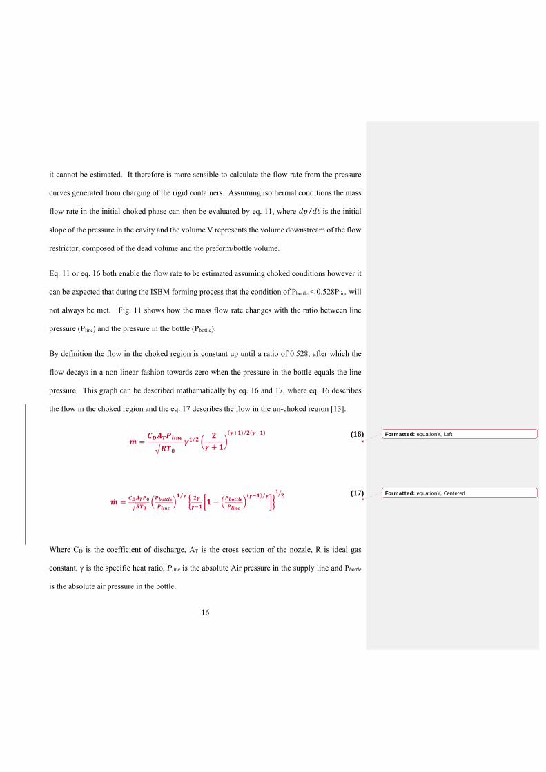
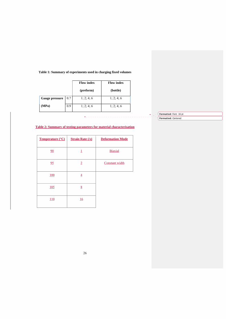