Measuring and modeling the dissolution of nonideally

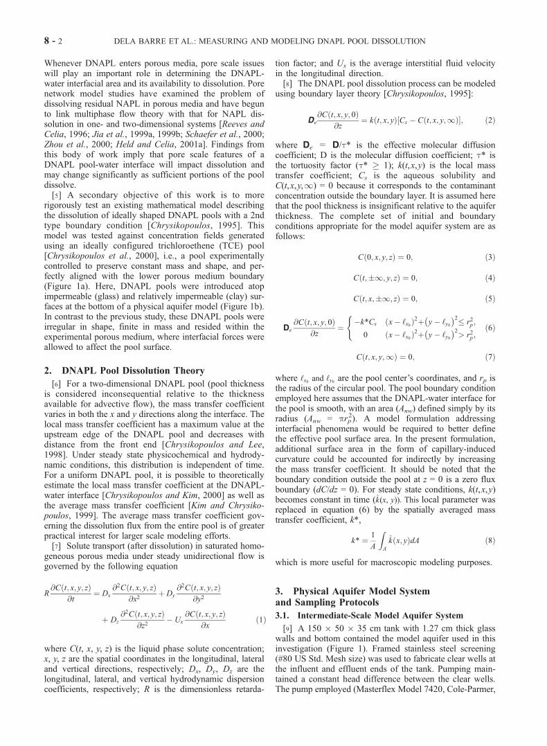
Measuring and modeling the dissolution of nonideally shaped dense

nonaqueous phase liquid pools in saturated porous media

Brian K. Dela Barre1 and Thomas C. Harmon

Department of Civil and Environmental Engineering, University of California, Los Angeles, California, USA

Constantinos V. Chrysikopoulos

Department of Civil and Environmental Engineering, University of California, Irvine, California, USA

Received 23 February 2001; revised 16 February 2002; accepted 4 March 2002; published 3 August 2002.

[1] A three-dimensional physical aquifer model was used to study the dissolution of adense nonaqueous phase liquid (DNAPL) pool. The model aquifer comprised a packing ofhomogeneous, medium-sized sand and conveyed steady, unidirectional flow.Tetrachloroethene (PCE) pools were introduced within model aquifers atop glass- andclay-lined aquifer bottoms. Transient breakthrough at an interstitial velocity of 7.2 cm/h,and three-dimensional steady state concentration distributions at velocities ranging from0.4 to 7.2 cm/h were monitored over periods of 59 and 71 days for the glass- and clay-bottom experiments, respectively. Pool-averaged mass transfer coefficients were obtainedfrom the observations via a single-parameter fit using an analytical model formulated witha second type boundary condition to describe pool dissolution [Chrysikopoulos, 1995].Other model parameters (interstitial velocity, longitudinal and transverse dispersioncoefficients, and pool geometry) were estimated independently. Simulated and observeddissolution behavior agreed well, except for locations relatively close to the pool or theglass-bottom plate. Estimated mass transfer coefficients ranged from 0.15 to 0.22 cm/h,increasing weakly with velocity toward a limiting value. Pool mass depletions of 31 and43% for the glass- and clay-bottom experiments failed to produce observable changes inthe plumes and suggested that changes in pool interfacial area over the period of theexperiment were negligible. Dimensionless mass transfer behavior was quantified using amodified Sherwood number (Sh*). Observed Sh* values were found to be about 2–3times greater than values predicted by an existing theoretical mass transfer correlation,and 3–4 times greater than those estimated previously for an ideally configuredtrichloroethene (TCE) pool (circular and smooth). It appeared that the analytical model’sfailure to account for pore-scale pool-water interfacial characteristics and larger scale poolshape irregularities biased the Sh* estimates toward greater values. INDEX TERMS: 1831

Hydrology: Groundwater quality; 1832 Hydrology: Groundwater transport; KEYWORDS: DNAPL, pool,

dissolution, mass transfer, three-dimensional

1. Introduction

[2] Dense nonaqueous phase liquid (DNAPL) can act as along-term source of groundwater contamination. The natureof a contaminant plume emanating from the DNAPL is aresult of the interplay between dissolution at the DNAPL-water interface, the interfacial area and its availability to theflow regime, and advection-dispersion processes in hetero-geneous porous media [Miller et al., 1998; Khachikian andHarmon, 2000]. DNAPL entrapped in a porous medium isconventionally categorized as a distribution of residualganglia or as pooled bodies. The latter occur when thepathway of a migrating DNAPL is impeded by a lowpermeability geologic unit. This research investigates thecontrolled dissolution of a pooled DNAPL.

[3] A body of theoretical work has shown that DNAPLpools have the potential to persist in the environment due totheir relatively low surface-to-volume ratio [Johnson andPankow, 1992; Chrysikopoulos et al., 1994; Chrysikopoulos,1995; Holman and Javandel, 1996; Lee and Chrysikopou-los, 1998; Kim and Chrysikopoulos, 1999]. Intermediate-scale box experiments [Pfannkuch, 1984; Anderson et al.,1992; Saba and Illangasekare, 2000; Chrysikopoulos et al.,2000] employing realistic DNAPL configurations have beenused to link laboratory and field observations by providingcontrolled three-dimensional data sets for model testing.Early experimental work on pool dissolution qualitativelycorroborates dissolution theory [Chrysikopoulos et al., 1994;Pearce et al., 1994; Voudrias and Yeh, 1994; Whelan et al.,1994]. However, data from such experiments are relativelysparse and inadequate to conclusively quantify the dissolu-tion rate from pools in three dimensions.[4] The primary goal of this research is to observe the

controlled dissolution of DNAPL pools into an overlyingporous medium, and to quantify the longevity of such pools.

1Now at Tetra Tech EM Inc., Reno, Nevada, USA.

Copyright 2002 by the American Geophysical Union.0043-1397/02/2001WR000444$09.00

8 - 1

WATER RESOURCES RESEARCH, VOL. 38, NO. 8, 10.1029/2001WR000444, 2002

Whenever DNAPL enters porous media, pore scale issueswill play an important role in determining the DNAPL-water interfacial area and its availability to dissolution. Porenetwork model studies have examined the problem ofdissolving residual NAPL in porous media and have begunto link multiphase flow theory with that for NAPL dis-solution in one- and two-dimensional systems [Reeves andCelia, 1996; Jia et al., 1999a, 1999b; Schaefer et al., 2000;Zhou et al., 2000; Held and Celia, 2001a]. Findings fromthis body of work imply that pore scale features of aDNAPL pool-water interface will impact dissolution andmay change significantly as sufficient portions of the pooldissolve.[5] A secondary objective of this work is to more

rigorously test an existing mathematical model describingthe dissolution of ideally shaped DNAPL pools with a 2ndtype boundary condition [Chrysikopoulos, 1995]. Thismodel was tested against concentration fields generatedusing an ideally configured trichloroethene (TCE) pool[Chrysikopoulos et al., 2000], i.e., a pool experimentallycontrolled to preserve constant mass and shape, and per-fectly aligned with the lower porous medium boundary(Figure 1a). Here, DNAPL pools were introduced atopimpermeable (glass) and relatively impermeable (clay) sur-faces at the bottom of a physical aquifer model (Figure 1b).In contrast to the previous study, these DNAPL pools wereirregular in shape, finite in mass and resided within theexperimental porous medium, where interfacial forces wereallowed to affect the pool surface.

2. DNAPL Pool Dissolution Theory

[6] For a two-dimensional DNAPL pool (pool thicknessis considered inconsequential relative to the thicknessavailable for advective flow), the mass transfer coefficientvaries in both the x and y directions along the interface. Thelocal mass transfer coefficient has a maximum value at theupstream edge of the DNAPL pool and decreases withdistance from the front end [Chrysikopoulos and Lee,1998]. Under steady state physicochemical and hydrody-namic conditions, this distribution is independent of time.For a uniform DNAPL pool, it is possible to theoreticallyestimate the local mass transfer coefficient at the DNAPL-water interface [Chrysikopoulos and Kim, 2000] as well asthe average mass transfer coefficient [Kim and Chrysiko-poulos, 1999]. The average mass transfer coefficient gov-erning the dissolution flux from the entire pool is of greaterpractical interest for larger scale modeling efforts.[7] Solute transport (after dissolution) in saturated homo-

geneous porous media under steady unidirectional flow isgoverned by the following equation

R@C t; x; y; zð Þ

@t¼ Dx

@2C t; x; y; zð Þ@x2

þ Dy

@2C t; x; y; zð Þ@y2

þ Dz

@2C t; x; y; zð Þ@z2

� Ux

@C t; x; y; zð Þ@x

ð1Þ

where C(t, x, y, z) is the liquid phase solute concentration;x, y, z are the spatial coordinates in the longitudinal, lateraland vertical directions, respectively; Dx, Dy, Dz are thelongitudinal, lateral, and vertical hydrodynamic dispersioncoefficients, respectively; R is the dimensionless retarda-

tion factor; and Ux is the average interstitial fluid velocityin the longitudinal direction.[8] The DNAPL pool dissolution process can be modeled

using boundary layer theory [Chrysikopoulos, 1995]:

De

@C t; x; y; 0ð Þ@z

¼ k t; x; yð Þ Cs � C t; x; y;1ð Þ½ �; ð2Þ

where De = D/t* is the effective molecular diffusioncoefficient; D is the molecular diffusion coefficient; t* isthe tortuosity factor (t* 1); k(t,x,y) is the local masstransfer coefficient; Cs is the aqueous solubility andC(t,x,y,1) = 0 because it corresponds to the contaminantconcentration outside the boundary layer. It is assumed herethat the pool thickness is insignificant relative to the aquiferthickness. The complete set of initial and boundaryconditions appropriate for the model aquifer system are asfollows:

C 0; x; y; zð Þ ¼ 0; ð3Þ

C t;1; y; zð Þ ¼ 0; ð4Þ

C t; x;1; zð Þ ¼ 0; ð5Þ

De

@C t; x; y; 0ð Þ@z

¼�k*Cs x� ‘x0ð Þ2þ y� ‘y0

� �2� r2p;

0 x� ‘x0ð Þ2þ y� ‘y0� �2

> r2p;

(ð6Þ

C t; x; y;1ð Þ ¼ 0; ð7Þ

where ‘x0 and ‘y0 are the pool center’s coordinates, and rp isthe radius of the circular pool. The pool boundary conditionemployed here assumes that the DNAPL-water interface forthe pool is smooth, with an area (Anw) defined simply by itsradius (Anw = prp

2). A model formulation addressinginterfacial phenomena would be required to better definethe effective pool surface area. In the present formulation,additional surface area in the form of capillary-inducedcurvature could be accounted for indirectly by increasingthe mass transfer coefficient. It should be noted that theboundary condition outside the pool at z = 0 is a zero fluxboundary (dC/dz = 0). For steady state conditions, k(t,x,y)becomes constant in time (k̂(x, y)). This local parameter wasreplaced in equation (6) by the spatially averaged masstransfer coefficient, k*,

k* ¼ 1

A

ZA

k̂ x; yð ÞdA ð8Þ

which is more useful for macroscopic modeling purposes.

3. Physical Aquifer Model Systemand Sampling Protocols

3.1. Intermediate-Scale Model Aquifer System

[9] A 150 � 50 � 35 cm tank with 1.27 cm thick glasswalls and bottom contained the model aquifer used in thisinvestigation (Figure 1). Framed stainless steel screening(#80 US Std. Mesh size) was used to fabricate clear wells atthe influent and effluent ends of the tank. Pumping main-tained a constant head difference between the clear wells.The pump employed (Masterflex Model 7420, Cole-Parmer,

8 - 2 DELA BARRE ET AL.: MEASURING AND MODELING DNAPL POOL DISSOLUTION

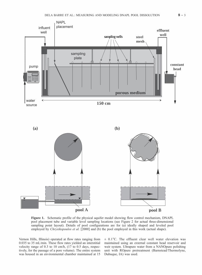
Vernon Hills, Illinois) operated at flow rates ranging from0.035 to 35 mL/min. These flow rates yielded an interstitialvelocity range of 0.3 to 10 cm/h, (17 to 0.5 days, respec-tively, for the passage of a pore volume). The entire systemwas housed in an environmental chamber maintained at 15

± 0.1�C. The effluent clear well water elevation wasmaintained using an external constant head reservoir andweir system. Ultrapure water from a NANOpure polishingunit with ROpure pretreatment (Barnstead/Thermolyne,Dubuque, IA) was used.

Figure 1. Schematic profile of the physical aquifer model showing flow control mechanism, DNAPLpool placement tube and variable level sampling locations (see Figure 2 for actual three-dimensionalsampling point layout). Details of pool configurations are for (a) ideally shaped and leveled poolemployed by Chrysikopoulos et al. [2000] and (b) the pool employed in this work (actual shape).

DELA BARRE ET AL.: MEASURING AND MODELING DNAPL POOL DISSOLUTION 8 - 3

[10] Two packing configurations were employed: homo-geneous sand supported by the glass tank-bottom and thesame homogeneous sand supported by a clay layer. Thematerial employed to fabricate the aquifer was #60 Lonestarsand (U.S. std. sieve size, Lonestar Sand, Monterey, CA).Grain sizes larger than about 0.425 mm (#40 U.S. Std. Sieve)were removed prior to packing. The geometric mean graindiameter of the resulting sand was 0.33 mm. The claymaterial comprised a pliable mixture of montmorillonite,kaolinite and smectite placed and leveled in a 1-cm thicklayer along the tank bottom. For both the glass- and clay-bottom experiments, the sand was placed in 2–3 cm liftsunder a water head of approximately 5–10 cm to a totalpacking depth of 20 cm. This configuration resulted in apacked volume of about 115,200 cm3 (120 � 48 � 20 cm).The tank was then filled with water (several cm above theupper level of packing) and left overnight to settle andsaturate. Following this initial saturation, the media wasphysically agitated by inserting a mechanically vibrated,5 mm diameter aluminum rod on 5 cm intervals. The finalporosity of the model aquifer was determined to be 0.38, andthe bulk density was determined to be 1.60 g/cm3. The waterlevel stabilized to an average saturated depth of 13 cm. Thesystem was then flushed at maximum velocity until theeffluent clear well was free of suspended fine material.[11] A Plexiglas grid of potential well locations anchored

immediately above the porous medium fixed the horizontallocation of sampling needles in terms of the coordinatesystem assigned for modeling purposes (Figure 2). Thirty-five observation ports were installed in the experimentalaquifer to allow periodic sampling of concentrations resultingfrom tracer injection or pool dissolution. Each port con-sisted of a 20-gauge stainless steel needle (0.58 mm innerdiameter, Hamilton Syringe, Reno, Nevada) guided throughholes in the support grid and anchored to the surface. Wireinserted in the needle during the placement process pre-vented clogging. The sampling points were fixed at eleva-

tions ranging from 0.5 to 3.0 cm above the glass or clayaquifer bottoms as designated in Figure 2. These elevationswere selected on the basis of preliminary model simulationsusing reasonable parameter estimates [Lee and Chrysiko-poulos, 1998; Kim and Chrysikopoulos, 1999], and on thepractical detection limits for organic solutes (discussedbelow). A small stream of 200 mg/L sodium azide solutionwas introduced to the influent clear well to inhibit biologicalgrowth.

3.2. Estimating Hydrodynamic Dispersion andSorption Parameters

[12] Model sensitivity analysis for one-dimensional sys-tems has demonstrated that the effluent concentrations areinsensitive to dispersivity values in the range of 0.01 to 1cm [Powers et al., 1991; Pennell et al., 1993]. In multi-dimensional systems, dispersion plays a critical role indetermining the shape of the plume emanating from aDNAPL. Thus, accurate estimates of mass transfer ratecoefficients for DNAPL pools require accurate dispersionparameter estimates. Pulse-input tracer tests were used toquantify local interstitial velocities. A comparison of pulsetravel times for different regions and elevations in the boxverified that a uniform flow field had been achieved. Localhorizontal velocity values were in agreement with the bulkinterstitial velocity values estimated using the aquiferdimensions and flow rate. Preliminary tests demonstratedthat the pulse-input tracer breakthrough curve shapes wereeasily biased by over-sampling, and therefore not useful forquantifying dispersion. Instead, dispersion coefficient valuesfor the model aquifer were estimated using step-inputbreakthrough tracer tests. The stationary tail offers theadvantage of being insensitive to sampling and highlysensitive to the transverse dispersion coefficients. Theconcentration front, which is not as susceptible to thesampling frequency problem as a pulse signal, is moresensitive to the longitudinal dispersion parameter.

Figure 2. Plan view of the model aquifer sampling plate showing active sampling locations in terms ofthe coordinate system used in the simulations. The numbers denote the elevation (z coordinate) of thesampling point above the aquifer bottom.


[13] Dispersion coefficients were determined by fittingthe observed step breakthrough response to an advection-dispersion transport model for a conservative, nonsorbingsolute in a homogeneous porous medium subject to unidirec-tional flow and three-dimensional dispersion [Chrysikopou-los et al., 2000]. The fits were optimized by coupling thedispersion model solution to the parameter optimizing rou-tine PEST [Doherty et al., 1994]. PEST employs the max-imum neighborhood approach [Marquardt, 1959, 1963],which combines steepest descent and the Gauss-Newtonmethods. Here, the longitudinal and transverse dispersioncoefficients were fitted, assuming equal horizontal (Dy) andvertical (Dz) transverse contributions.[14] The relatively low amount of dispersion observed in

the tracer tests implied that the diffusive contribution wassignificant and required quantification. The tortuosity (t*)value was estimated by monitoring the transport of a tracer(tritiated water) solute within the same sand-packing underquiescent conditions. The effective tortuosity factor for therelatively nonrestrictive interparticle pores associated with awell-sorted sand will be reasonably independent of the

tracer molecule. Thus we chose to use tritiated water, asopposed to the solute of interest (PCE), because of thegreater cost and safety concerns associated with carbon-14labeled PCE. A one-dimensional diffusion column wasfabricated using a brass sleeve (2.54 cm in diameter)situated atop a screened, well-stirred reservoir. The box-packing procedure described earlier was replicated in thissystem. A support apparatus was fabricated for anchoring amicrosyringe to the diffusion column to facilitate thecollection of 2 mL samples as a function of depth [DelaBarre, 1999]. Concentration profiles were measured at 7and 21 days and modeled using the solution to the equationfor diffusive transport from a source of limited volume intoa semi-infinite column [Crank, 1975]. Results for bothprofiles collected yielded a tortuosity estimate of 1.7 for thetritiated water [Dela Barre, 1999], which is reasonable for asandy medium [Perkins and Johnston, 1963]. Estimating anaqueous diffusivity (D) value of 7.1� 10�6 cm2/s at 15�C forPCE [Wilke and Chang, 1955], and assuming the sametortuosity value for both solutes, the corresponding De valuefor PCE is 4.2 � 10�6 cm2/s (0.015 cm2/h).

Table 1. Summary of PCE Dissolution Model Parameter Estimates and Resulting Fitted

Values of the Pool-Averaged Mass Transfer Coefficient (k*)

Parameter Estimatea Source of Estimate

Cs 180 ± 10 mg/L batch measurementrp, glass bottom 1.9 ± 0.1 cm visual measurementrp, clay bottom 2.5 ± 0.1 cm clay depression sizeD 0.026 ± 0.002 cm2/h Wilke and Chang [1955]t* 1.7 ± 0.05 (dimensionless) column diffusion experimentsUx

Slow 0.4 ± 0.003 cm/h pulse tracer tests; Pex = 7.6, Pey = 38Medium 2.6 ± 0.005 pulse tracer tests; Pex = 8.5, Pey = 71Fast 7.2 ± 0.007 pulse tracer tests; Pex = 8.6, Pey = 86Clay bottom 5.6 ± 0.007 pulse tracer tests; Pex = 11.2, Pey = 108

Dx

Low 0.10 ± 0.008 cm2/h step tracer tests (aL = 0.22 ± 0.02 cm)Medium 0.58 ± 0.05 step tracer tests (aL = 0.22 ± 0.02 cm)High 1.59 ± 0.14 step tracer tests (aL = 0.22 ± 0.02 cm)Clay bottom 1.25 ± 0.11 step tracer tests (aL = 0.22 ± 0.02 cm)

Dy = Dz

Low 0.02 ± 0.002 cm2/h step tracer tests (aT = 0.02 ± 0.0015 cm)equation (16)a

Medium 0.07 ± 0.005 step tracer tests (aT = 0.02 ± 0.0015 cm)equation (16)a

High 0.16 ± 0.011 step tracer tests (aT = 0.02 ± 0.0015 cm)equation (16)a

Clay bottom 0.13 ± 0.009 step tracer tests (aT = 0.02 ± 0.0015 cm)equation (16)a

k*Low 0.15 ± 0.02 cm/h single-parameter fit to pool dissolution

modelb

Medium 0.21 ± 0.03 single-parameter fit to pool dissolutionmodelb

High 0.22 ± 0.04 single-parameter fit to pool dissolutionmodelb

Clay bottom 0.21 ± 0.06 single-parameter fit to pool dissolutionmodelb

aError (±) bounds for parameters: Cs, standard deviation (n = 6); rp visual estimate; D, relative errorassociated with Wilke-Chang expression (7.5%); t*, 95% confidence interval (CI) for optimizedparameter in fit to diffusion data [Dela Barre, 1999]; Ux, standard deviation (n = 7 for each velocity).Dispersion coefficients were estimated using Di = aiUx + De with error bounds estimated by propagatingthe error associated with the parameter estimates for dispersivity (95% CI for optimized parameter in fit tostep input tracer data).

bLow-velocity k* estimate based on single data set of 28 observations; medium, high, and clay bottomk* estimates are each the average duplicate data sets of 14 observations. Error bound on k* estimates arebased on fitting extremities achieved using minimum and maximum dispersion parameter values.


[15] The dispersion parameters used to model DNAPLpool dissolution results are summarized in Table 1. To arriveat the values indicated, the fitted dispersion coefficients andeffective diffusivity value from the tracer experiments werefirst used to estimate the porous medium dispersivity values(aL = 0.22 and aT = 0.02 cm) as per Bear [1972]. Thesedispersivity values are in good agreement with thoseobtained for a similar system [0.26 and 0.02 cm, Chrys-ikopoulos et al., 2000]. Given these dispersivity values,dispersion coefficients were calculable for the interstitialvelocities employed in the pool dissolution experiments.[16] The PCE sorption capacity of the sandwas determined

in batch samples contained in flame-sealed ampules [Ball andRoberts, 1991; Harmon and Roberts, 1994]. Triplicate sam-ples were equilibrated at each of five concentrations rangingfrom 1 mg/L to 50 mg/L. The resulting isotherm wasdescribed well by linear isotherm, and yielded a distributioncoefficient (Kd) of 0.30 mL/g. This Kd value corresponds to aretardation factor of approximately 2.3.

3.3. DNAPL Pool Placement and Organic SoluteSampling

[17] In the first experiment, a single DNAPL pool wasplaced on the glass tank-bottom by pumping pure tetrachlor-oethene (PCE) through a 0.3 mm (inner diameter) glass tubepositioned during the packing procedure. In the secondexperiment, a PCE pool was placed in a 3 cm diameterdepression on top of the clay layer. In both cases, the tubefully penetrated the porous medium, contacting the bottomsurface at coordinates x = 7, y = 13 (Figure 2). Initially, theinjection system was filled with water to prevent air-intru-sion into the saturated media during placement. Pools wereinjected at a rate of about 6 mL/h while maintaining aconstant interstitial velocity (0.4 cm/h). After approximately1 mL (1.62 g) of PCE was placed at the bottom of themedium, the injection was halted and the tube was capped.For the case of the glass-bottom, capillary and gravitationalforces caused the pool to spread laterally along the bottom ofthe tank in a roughly circular pattern. The visually observedpool outline was traced with indelible ink on the bottom ofthe glass tank (Figure 1b). The area of the pool shape wasestimated to be about 11.3 ± 1.2 cm2. This corresponds to anominal diameter for a circular pool of 3.8 ± 0.2 cm, andimplies a pool thickness of slightly more than 0.1 mm. Forthe case of the clay-bottom, the pool was not observable, andwas assumed to be distributed evenly in the depression.[18] For the glass-bottom experiment, the velocity was

increased to 7.2 cm/h immediately after pool placement.Temporal sampling was carried out at the designated obser-vation point (Figure 2) approximately 73 cm downgradientof the pool to determine when steady state dissolutionconditions were achieved. Subsequent sampling was synop-tic and occurred at 4.5 12, 17, 31 and 59 days for interstitialvelocities of 7.2, 2.6, 7.2, 2.6 and 0.4 cm/h, respectively. Forthe clay-bottom experiment, synoptic sampling was under-taken 34 and 71 days after pool placement at a constantinterstitial velocity of 5.6 cm/h. The additional time for theclay-bottom experiment was intended to allow for equilibra-tion between the clay and the lower portions of the plume.All aqueous samples were collected using a 1 mL gas-tightsyringe. Approximately 30 to 40 mL of aqueous solutionwere purged from each well immediately prior to sample

collection. Sampling events began at downgradient welllocations and proceeded toward the pool to minimize theeffects of previous sample withdrawal on subsequent sam-pling events. For each sample, a 20 to 60 mL volume(determined gravimetrically) was withdrawn and deliveredto a 2 mL glass receiving vial. The smaller volumes weretaken near the centerline of the plume and deeper in theaquifer, where greater concentrations were expected. Thelarger volumes were collected on the periphery and at higherelevations. The entire system was allowed to recover for thepassage of two to three pore volumes prior to subsequentsampling events.[19] Samples from the model aquifer were prepared for

analysis using a micro-extraction protocol developed toaccommodate the limited sample volumes available in theseexperiments. Receiver vials contained 1.0 to 1.8 mLof pentane spiked with an internal standard (1-bromo,2-chloro-propane). Specific volumes were inversely relatedto the magnitude of the anticipated solute concentration.Samples were dispensed below the surface of the extractingsolvent to minimize volatilization losses. Prior to analysis,the pentane phase was transferred from the receiver vial to amicro-vial and capped using a crimped foil cap with Teflon/silicone septa. Sample PCE levels were quantified via auto-injection into a gas chromatograph (Hewlett Packard Model6890) equipped with an HP-624 column and electron capturedetector. The practical range of detection for PCE in themodel aquifer was from 0.5 to 80 mg/L. Samples observed tobe above the upper detection limit were diluted in greateramounts of pentane in subsequent sampling events.

4. Results and Discussion

[20] PCE breakthrough at the transient observation pointwas used to determine when steady state transport behaviorwas achieved during pool dissolution. The observed behavioris plotted in Figure 3. The vertical lines in Figure 3 denotethe synoptic sampling events (discussed below). Thesimulated transient portions of the breakthrough responsesin Figure 3 are clearly less dispersed relative to theobserved behavior. One possible source of this discrepancyis the effect of sorption. However, the primary (equili-brium) sorption effect is accounted for by the retardationfactor. Thus, this discrepancy is most likely an artifact ofthe high sampling frequency (roughly every 15 min) andlarger volumes (20–60 mL) required for analysis. Thissampling regime drew the contaminant front forward,creating early breakthrough. The sampling also appearedto enhance dilution at the other end of the breakthroughcurve such that a maximum concentration was notobserved until the sampling frequency was markedlydecreased. Sampling problems were less evident in thestep-input tracer tests because the tritiated water could beanalyzed with much lower sample withdrawals (2 mL).Thus, adjustment of the dispersion parameters to bettersimulate the front in Figure 3 would be inappropriate, andthe values estimated via the tracer tests were used.[21] The data in Figure 3 suggest that one to four days

were needed for the dissolving pool to deliver a steadyconcentration roughly 73 cm downgradient from the pool.For reference, one day at a rate of 7.2 cm/h corresponds toabout 2.5 pore volumes passing through this length of the


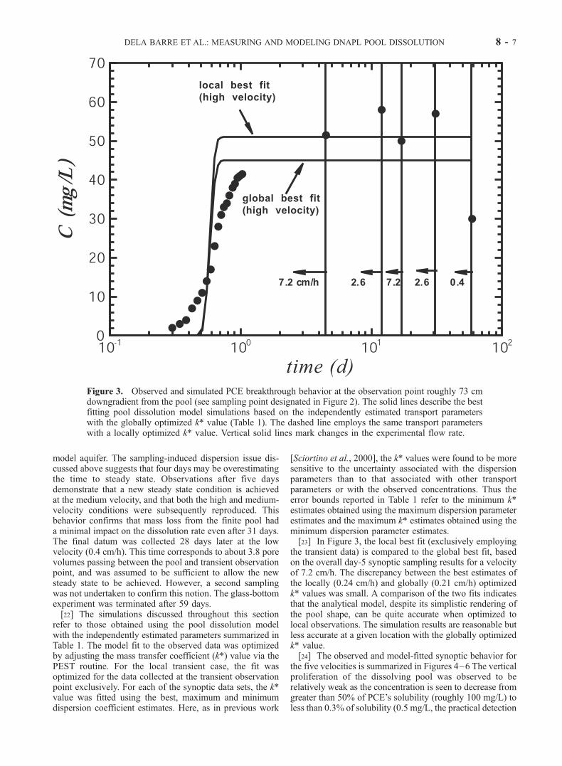
model aquifer. The sampling-induced dispersion issue dis-cussed above suggests that four days may be overestimatingthe time to steady state. Observations after five daysdemonstrate that a new steady state condition is achievedat the medium velocity, and that both the high and medium-velocity conditions were subsequently reproduced. Thisbehavior confirms that mass loss from the finite pool hada minimal impact on the dissolution rate even after 31 days.The final datum was collected 28 days later at the lowvelocity (0.4 cm/h). This time corresponds to about 3.8 porevolumes passing between the pool and transient observationpoint, and was assumed to be sufficient to allow the newsteady state to be achieved. However, a second samplingwas not undertaken to confirm this notion. The glass-bottomexperiment was terminated after 59 days.[22] The simulations discussed throughout this section

refer to those obtained using the pool dissolution modelwith the independently estimated parameters summarized inTable 1. The model fit to the observed data was optimizedby adjusting the mass transfer coefficient (k*) value via thePEST routine. For the local transient case, the fit wasoptimized for the data collected at the transient observationpoint exclusively. For each of the synoptic data sets, the k*value was fitted using the best, maximum and minimumdispersion coefficient estimates. Here, as in previous work

[Sciortino et al., 2000], the k* values were found to be moresensitive to the uncertainty associated with the dispersionparameters than to that associated with other transportparameters or with the observed concentrations. Thus theerror bounds reported in Table 1 refer to the minimum k*estimates obtained using the maximum dispersion parameterestimates and the maximum k* estimates obtained using theminimum dispersion parameter estimates.[23] In Figure 3, the local best fit (exclusively employing

the transient data) is compared to the global best fit, basedon the overall day-5 synoptic sampling results for a velocityof 7.2 cm/h. The discrepancy between the best estimates ofthe locally (0.24 cm/h) and globally (0.21 cm/h) optimizedk* values was small. A comparison of the two fits indicatesthat the analytical model, despite its simplistic rendering ofthe pool shape, can be quite accurate when optimized tolocal observations. The simulation results are reasonable butless accurate at a given location with the globally optimizedk* value.[24] The observed and model-fitted synoptic behavior for

the five velocities is summarized in Figures 4–6 The verticalproliferation of the dissolving pool was observed to berelatively weak as the concentration is seen to decrease fromgreater than 50% of PCE’s solubility (roughly 100 mg/L) toless than 0.3% of solubility (0.5 mg/L, the practical detection

Figure 3. Observed and simulated PCE breakthrough behavior at the observation point roughly 73 cmdowngradient from the pool (see sampling point designated in Figure 2). The solid lines describe the bestfitting pool dissolution model simulations based on the independently estimated transport parameterswith the globally optimized k* value (Table 1). The dashed line employs the same transport parameterswith a locally optimized k* value. Vertical solid lines mark changes in the experimental flow rate.


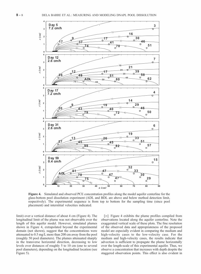
limit) over a vertical distance of about 4 cm (Figure 4). Thelongitudinal limit of the plume was not observable over thelength of this aquifer model. However, simulated plumesshown in Figure 4, extrapolated beyond the experimentaldomain (not shown), suggest that the concentrations wereattenuated to 0.5 mg/L more than 200 cm away from the pool(roughly 50 pool diameters). The plumes attenuated sharplyin the transverse horizontal direction, decreasing to lowlevels over distances of roughly 5 to 10 cm (one to severalpool diameters), depending on the longitudinal location (seeFigure 5).

[25] Figure 4 exhibits the plume profiles compiled fromobservations located along the aquifer centerline. Note theexaggerated vertical scale of these plots. The fine resolutionof the observed data and appropriateness of the proposedmodel are especially evident in comparing the medium andhigh-velocity cases to the low-velocity case. For themedium and high-velocity cases, the results indicate thatadvection is sufficient to propagate the plume horizontallyover the length-scale of this experimental aquifer. Thus, weobserve a concentration that increases with depth despite thestaggered observation points. This effect is also evident in

Figure 4. Simulated and observed PCE concentration profiles along the model aquifer centerline for theglass-bottom pool dissolution experiment (ADL and BDL are above and below method detection limit,respectively). The experimental sequence is from top to bottom for the sampling time (since poolplacement) and interstitial velocities indicated.


the fact that observed concentrations generally increasedafter the change from the high to the medium velocity. Forthe low-velocity case, the plume failed to propagate as far inthe horizontal direction, allowing for the accumulation ofhigher concentrations at many of the observation points. Onthe length-scale of this experiment, the overall effect was

that the staggered observations tended toward constantvalues (tracking the isoconcentration lines). The dynamicsdescribed by these observations are captured well by themodel fits based on the single adjustable parameter.[26] Local discrepancies between simulated and observed

profiles merit further discussion. The most prominent dis-

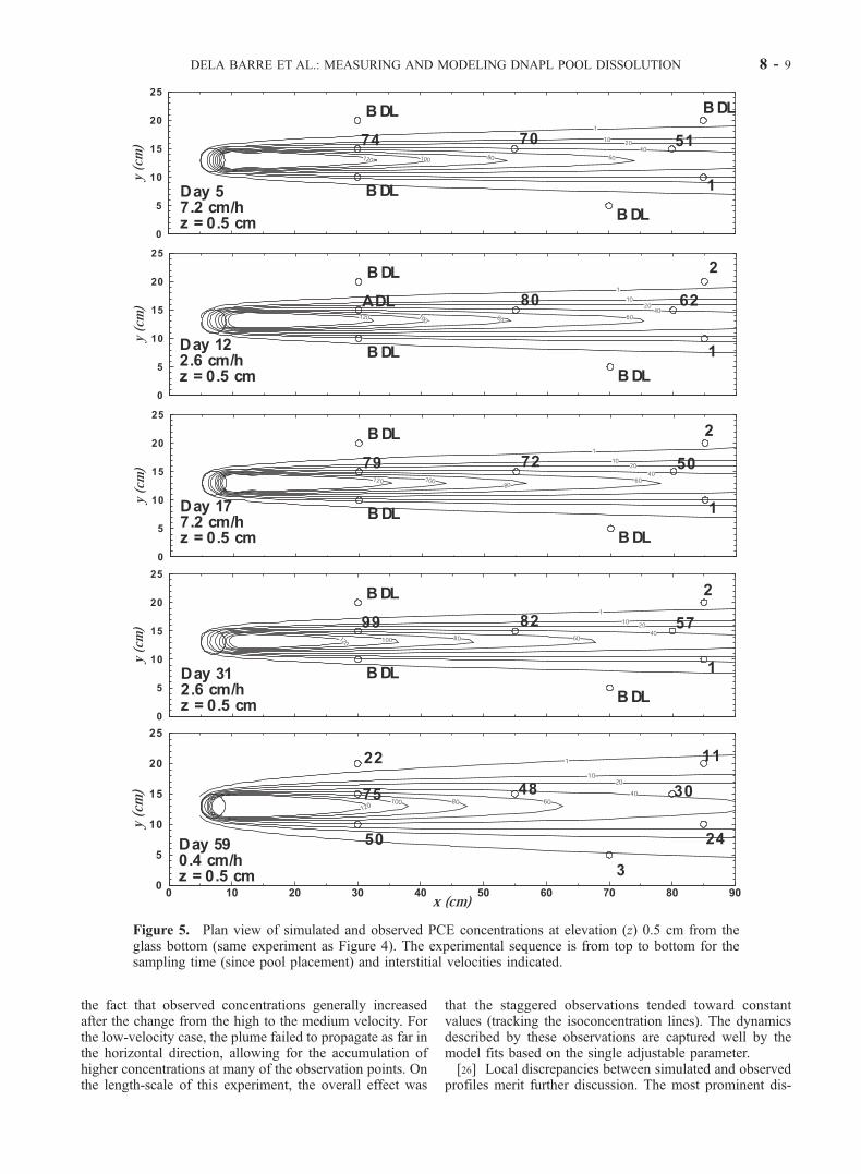
Figure 5. Plan view of simulated and observed PCE concentrations at elevation (z) 0.5 cm from theglass bottom (same experiment as Figure 4). The experimental sequence is from top to bottom for thesampling time (since pool placement) and interstitial velocities indicated.


crepancies for the medium and high velocities in Figure 4are found at the lowermost observation points. For the low-velocity case, observation points near the pool are at oddswith the model for all depths. One potential cause for thisdiscrepancy is that the solubility value measured for this

study was more than 20% lower than the 230 mg/L sug-gested by the data of Imhoff et al. [1997, Figure 3]. Using thegreater value in the dissolution simulations resulted inslightly lower k* values. For example, inputting 230 mg/Lfor the medium-velocity case produced a revised k* value of

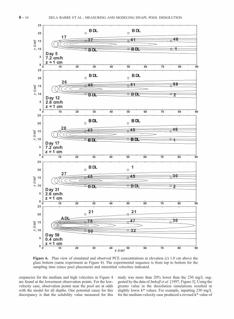
Figure 6. Plan view of simulated and observed PCE concentrations at elevation (z) 1.0 cm above theglass bottom (same experiment as Figure 4). The experimental sequence is from top to bottom for thesampling time (since pool placement) and interstitial velocities indicated.


0.19–0.20 cm/h (compared to 0.21–0.22 cm/h in Table 1).The quality of the fits was not improved as the revisedsimulations continued to fail to match at the near-pool anddeep observation points. Thus, it was concluded that thesolubility value measured here was sufficiently accurate. Amore likely reason for the discrepancies appears to beassociated with the difficulty in making accurate concentra-tion measurements in regions associated with steep concen-tration gradients. This problem pertains to observation pointinstallation, for horizontal and/or vertical deviations by aslittle as 1mm from intended locations will result in significantsampling errors in regions of steep gradient. A potentiallymore significant problem is inherent in modeling an irregu-larly shaped pool using the analytical model for the average(circular) pool shape (see pool rendering in Figure 1b).Sampling points downgradient of pool diameters greater thanthe average feel a stronger source than other regions; thosedowngradient of less-than-average diameters feel a weakersource. Simulations allowing for the adjustment of bothdispersion coefficients and k* values improved the qualityof the simulation at near-pool and low elevation samplingpoints, but at the expense of the more numerous elevatedobservations. Given the potential problems associated withsampling at these locations, the fitting exercises wererepeated while omitting these data. The mass transfer coef-ficient estimates were found to be insensitive to the presenceor absence of these data. This result is not surprising giventhe large number of observations used in fitting exercises (seefootnote to Table 1).[27] Figures 5 and 6 exhibit planar views of the same

plumes at elevations of 0.5 and 1.0 cm, respectively, above

the glass bottom. Agreement between the model andobserved concentrations is poor for the lower elevationfor all cases but the low velocity. This is not surprisinggiven that the centerline observations for these data sets arethe same as those used to develop the profiles in Figure 4.At the 1-cm elevation, there is good agreement between themodel and the observed concentrations. The systemdynamics discussed above are just as apparent from aplanar perspective, as the centerline concentrations arereasonably constant longitudinally for the medium andhigh velocities, but decrease longitudinally for the low-velocity case. Again, the dissolution model results are inaccord with this behavior.[28] Observation point density was insufficient to quan-

tify transverse horizontal plume expanse conclusively inmost cases. Nonquantifiable traces were observed along theplume edges, suggesting that the simulated plumes inFigures 5 and 6 represent a reasonable estimate of theplume width for the medium- and high-velocity cases.However, the low-velocity case indicates that the plume issubstantially wider than the best fitting simulation wouldindicate. Closer inspection of the off-centerline low-velocityobservations (y = 10 cm and y = 20 cm) also confirms adegree of asymmetry in observed plume favoring the side‘‘above’’ the centerline (y = 20 cm). This result is indicativeof the irregular pool shape (Figure 1b), which may havecontributed a stronger mass flux on this side of the system.[29] The clay-bottom experiment yielded the data shown

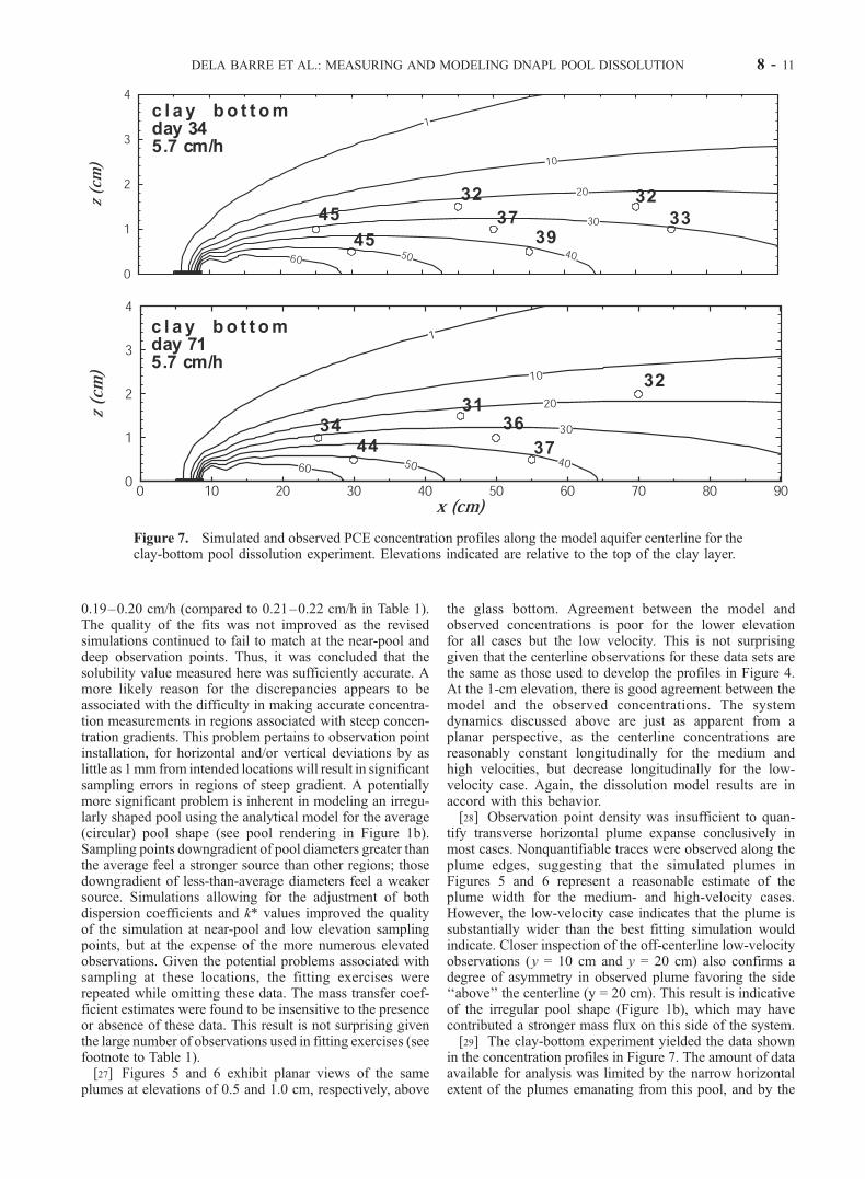
in the concentration profiles in Figure 7. The amount of dataavailable for analysis was limited by the narrow horizontalextent of the plumes emanating from this pool, and by the

Figure 7. Simulated and observed PCE concentration profiles along the model aquifer centerline for theclay-bottom pool dissolution experiment. Elevations indicated are relative to the top of the clay layer.


occurrence of needle-clogging (due to particle intrusionduring sampling). The model fits to the two data sets yieldedsimilar k* values that were consistent with those obtainedfrom the glass-bottom experiments at the high velocity. Incontrast to the high-velocity glass-bottom results, the 0.5-cmelevation clay-bottom observations were slightly less thanbest fitting simulation would dictate. This finding suggeststhat diffusion of the aqueous PCE into the adjacent clay layermay have played a role. However, the lag-time prior tosampling in the clay-bottom experiment was intended toallow for this behavior. Furthermore, the discrepancybetween the model and the simulation in these locations isrelatively minor. These points suggest that the two mediawere nearly in equilibrium by the time sampling occurred.

5. Pool Mass Depletion Estimates

[30] Using the estimated mass transfer coefficients it ispossible to estimate the mass flux from the pool using Fick’sfirst law as expressed in equation (6). The overall mass lossfrom the pool can then be estimated as the product of theflux and the pool area:

dM

dt¼ �k*CsA ð9Þ

where M is the mass of PCE in the pool and A is the pool’ssurface area. Integrating equation (9) over the course of theexperiments and accounting for the different k* values at the

different velocities yields mass losses of about 0.5 g over 51days and 0.7 g over 71 days for the glass- and clay-bottomexperiments, respectively. These losses correspond to about31% and 43% of the initial pool masses. Given that thestationary nature of the plumes was confirmed for all but thelow-velocity experiment (which corresponded to about 4additional pore volumes beyond the termination of thesecond medium-velocity experiment), it was concluded thatthe corresponding change in pool shape and interfacial areawas insufficient to markedly alter the dissolution rate.

6. Correlating Mass Transfer Behavior withHydrodynamic Conditions

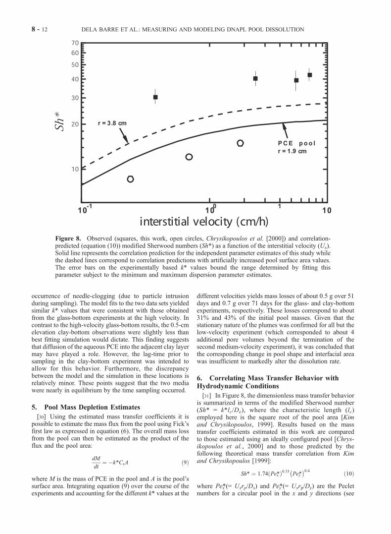
[31] In Figure 8, the dimensionless mass transfer behavioris summarized in terms of the modified Sherwood number(Sh* = k*lc/De), where the characteristic length (lc)employed here is the square root of the pool area [Kimand Chrysikopoulos, 1999]. Results based on the masstransfer coefficients estimated in this work are comparedto those estimated using an ideally configured pool [Chrys-ikopoulos et al., 2000] and to those predicted by thefollowing theoretical mass transfer correlation from Kimand Chrysikopoulos [1999]:

Sh* ¼ 1:74 Pex*ð Þ0:33 Pey*� �0:4 ð10Þ

where Pex*(= Uxrp/Dx) and Pey*(= Uxrp/Dy) are the Pecletnumbers for a circular pool in the x and y directions (see

Figure 8. Observed (squares, this work, open circles, Chrysikopoulos et al. [2000]) and correlation-predicted (equation (10)) modified Sherwood numbers (Sh*) as a function of the interstitial velocity (Ux).Solid line represents the correlation prediction for the independent parameter estimates of this study whilethe dashed lines correspond to correlation predictions with artificially increased pool surface area values.The error bars on the experimentally based k* values bound the range determined by fitting thisparameter subject to the minimum and maximum dispersion parameter estimates.


Table 1 for Peclet number estimates). The Sh* valuesestimated here are two to three times greater than thosepredicted by the correlation parameterized by the best fittingvalues for this work, and roughly three to four times greaterthan those estimated in the previous study of an ideallyconfigured pool.[32] The relatively large discrepancy between the Sh*

values observed in this work and those from the previousinvestigations may be due in part to experimental errors ofthe type mentioned previously (e.g., sampling point mis-alignment, and the idealized pool configuration assumed bythe analytical model). Another possible error source notdiscussed previously could be localized vertical velocitycomponents and the associated enhancement of the disper-sivity in the vicinity of a DNAPL-impacted zone [Pennell etal., 1993]. These types of effects are not accounted for inthis work and their presence would also bias results towardgreater Sh* values.[33] More important than experimental errors discussed

above are the limitations imposed by the ideally shaped poolmodeling assumptions. Whenever a pool develops in aporous medium, pore level effects will tend to increase theinterfacial area relative to the smooth approximation. Largerscale interfacial effects are evident in the deviation fromcircular behavior seen in Figure 1b. The present model willtend to overestimate the mass transfer coefficient in an effortto compensate for the underestimated surface area. Specificinterfacial areas calculated for residual DNAPL using porenetwork models range from about 0.3 to 2 mm2/mm3 [Heldand Celia, 2001b]. Estimating our effective porous mediumvolume as the observed pool area (11.3 cm2)multiplied by thepool thickness (estimated as DNAPL volume injected (1 mL)divided by (the pool area times the porosity)) andmultiplyingthis overall volume by 2 mm2/mm3 yields an Anw value forthe pool of 12 cm2, very similar to the smooth pool approx-imation of 11.3 cm2. Assuming that the pool is thicker, say1 mm in the extreme, the resulting Anw estimate for the poolincreases to 24 cm2. Thus the pore scale effects may besignificant here, but the larger scale effects causing thenoncircular pool shape appear to be equally or more impor-tant in this system.

7. Summary and Conclusions

[34] Aqueous plumes emanating from realistic DNAPLpools placed atop glass and clay aquifer-bottoms weremonitored at downgradient sampling points. All requiredtransport parameters, with the exception of the pool-averagemass transfer coefficient (k*), were estimated independently.With adjustment of the average mass transfer coefficientvalue, the analytical solution for pool dissolution in ahomogeneous porous medium was found to adequatelydescribe the observed PCE plume. Specific conclusionsstemming from this work are as follows.1. Despite the finite pool volume (1 mL), observed

plumes achieved a quasi-steady state distribution overextended time periods (months). A relatively constantmass flux developed at the pool-groundwater interfaceacting as the plume source. This flux was sufficiently slowthat the effect of mass loss on pool geometry (effectivedissolution surface) was minimal over the course of theseexperiments. Thus, it appears that pool-water interfacial

areas change on a slower timescale than do residual-waterinterfacial areas.2. Pool dissolution behavior was reasonably well-

modeled using boundary layer theory (second typeboundary condition) assuming a simplistic (circular) poolshape. The model was especially successful in simulatingthe vertical and longitudinal concentration profile near thecenterline of the plume. However, local discrepanciesbetween the model and observations were significant,especially near the pool. These discrepancies may be theresult of pore scale surface curvature and larger scaleshape irregularities that could not be simulated using thepresent model.3. Estimated mass transfer coefficient (k*) values were

two to three times greater than values predicted by atheoretically based mass transfer correlation for elliptical/circular pools and three to four times greater than thoseestimated in a dissolution study involving an ideallyconfigured pool. The most likely cause of these dis-crepancies was the pool dissolution model’s failure toaddress interfacial issues associated with the emplacedpool and overcompensation in the form of elevated masstransfer coefficients.[35] The rates and steady contaminant distributions sum-

marized here should be useful to contaminant hydrogeol-ogists in search of more accurate source depictions forlarger-scale transport models. For example, it is likely thatalternative boundary conditions (first- and third-type) canbe used to adequately model the pool dissolution process.The appropriate conditions and parameters under whichalternative boundary conditions are valid need to beidentified. Additional future research aimed at elucidatingthe connection between pool dissolution and pore-scalemechanisms defining the pool-water interface is clearlywarranted. Such work will become increasingly compli-cated in heterogeneous porous media.

[36] Acknowledgments. This work was supported by a grant fromthe U.S. Environmental Protection Agency’s Office of ExploratoryResearch (award R-823579-01-0). The content of this manuscript has notbeen subjected to the Agency’s review and no official endorsement shouldbe inferred. The authors thank Priti Brahma for measuring PCE solubility atthe temperature of the study.

ReferencesAnderson, M. R., R. L. Johnson, and J. F. Pankow, Dissolution of densechlorinated solvents into ground-water, 1, Dissolution from a well-de-fined residual source, Ground Water, 30(2), 250–256, 1992.

Ball, W. P., and P. V. Roberts, Long-term sorption of halogenated organicchemicals by aquifer material, 1, Equilibrium, Environ. Sci. Technol.,25(7), 1223–1237, 1991.

Bear, J., Dynamics of Flow in Porous Media, Elsevier Sci., New York,1972.

Chrysikopoulos, C. V., Three-dimensional analytical models of contaminanttransport from nonaqueous phase liquid pool dissolution in saturatedsubsurface formations, Water Resour. Res., 31(4), 1137–1145, 1995.

Chrysikopoulos, C. V., and T.-J. Kim, Local mass transfer correlations fornon-aqueous phase liquid pool dissolution in saturated porous media,Transp. Porous Media, 38(1/2), 167–187, 2000.

Chrysikopoulos, C. V., and K. Y. Lee, Contaminant transport resulting frommulticomponent nonaqueous phase liquid pool dissolution in three-di-mensional subsurface formations, J. Contam. Hydrol., 31(1–2), 1–21,1998.

Chrysikopoulos, C. V., E. A. Voudrias, and M. M. Fyrillas, Modeling ofcontaminant transport resulting from dissolution of nonaqueous phaseliquid pools in saturated porous media, Transp. Porous Media, 16(2),125–145, 1994.


Chrysikopoulos, C. V., K. Y. Lee, and T. C. Harmon, Dissolution of a well-defined trichloroethylene pool in saturated porous media: Experimentaldesign and aquifer characterization, Water Resour. Res., 36(7), 1687–1696, 2000.

Crank, J., The Mathematics of Diffusion, Oxford Univ. Press, New York,1975.

Dela Barre, B. K., Mass transfer coefficient estimation for dense nonaqu-eous phase liquid pool dissolution using a three-dimensional physicalaquifer model, Ph.D. dissertation, 118 pp., Univ. of Calif., Los Angeles,1999.

Doherty, J., L. Brebber, and P. Whyte, PEST: Model-independent parameterestimation, Watermark Computing, Brisbane, Australia, 1994.

Harmon, T. C., and P. V. Roberts, A comparison of intraparticle sorptionand desorption rates for a halogenated alkene in a sandy aquifer material,Environ. Sci. Technol., 28(9), 1650–1660, 1994.

Held, R. J., and M. A. Celia, Pore-scale modeling and upscaling of non-aqueous phase liquid mass transfer, Water Resour. Res., 37(3), 539–549,2001a.

Held, R. J., and M. A. Celia, Modeling support of functional relationshipsbetween capillary pressure, saturation, interfacial area and common lines,Adv. Water Res., 24, 325–343, 2001b.

Holman, H. Y. N., and I. Javandel, Evaluation of transient dissolution ofslightly water-soluble compounds from a light nonaqueous phase liquidpool, Water Resour. Res., 32(4), 915–923, 1996.

Imhoff, P. T., A. Frizzell, and C. T. Miller, Evaluation of the thermal effectson the dissolution of a nonaqueous phase liquid in porous media, En-viron. Sci. Technol., 31, 1615–1622, 1997.

Jia, C., K. Shing, and Y. C. Yortsos, Visualization and simulation of NAPLsolubilization in pore networks, J. Contam. Hydrol., 35, 363–387,1999a.

Jia, C., K. Shing, and Y. C. Yortsos, Advective mass transfer from station-ary sources in porous media, Water Resour. Res., 35(11), 3239–3251,1999b.

Johnson, R. L., and J. F. Pankow, Dissolution of dense chlorinated solventsinto groundwater, 2, Source functions for pools of solvent, Environ. Sci.Technol., 26(5), 896–901, 1992.

Khachikian, C. S., and T. C. Harmon, Nonaqueous phase liquid dissolutionin porous media: Current state of knowledge and research needs, Transp.Porous Media, 38(1/2), 3–28, 2000.

Kim, T.-J., and C. V. Chrysikopoulos, Mass transfer correlations for non-aqueous phase liquid pool dissolution in saturated porous media, WaterResour. Res., 35(2), 449–459, 1999.

Lee, K. Y., and C. V. Chrysikopoulos, NAPL pool dissolution in stratifiedand anisotropic porous formations, J. Environ. Eng., 124(9), 851–862,1998.

Marquardt, D. W., Solution of nonlinear chemical engineering models,Chem. Eng. Progr., 55(6), 65–70, 1959.

Marquardt, D. W., An algorithm for least-squares estimation of nonlinearparameters, J. Soc. Indust. Appl. Math., 11(2), 431–441, 1963.

Miller, C. T., G. Christakos, P. T. Imhoff, J. F. McBride, J. A. Pedit, andJ. A. Trangenstein, Multiphase flow and transport modeling in hetero-

geneous media: Challenges and approaches, Adv. Water Res., 21(2),77–120, 1998.

Pearce, A. E., E. A. Voudrias, and M. P. Whelan, Dissolution of TCE andTCA pools in saturated subsurface systems, J. Environ. Eng., 120(5),1191–1206, 1994.

Pennell, K. D., L. M. Abriola, and W. J. Weber, Surfactant-enhanced solu-bilization of residual dodecane in soil columns, 1, Experimental investi-gation, Environ. Sci. Technol., 27(12), 2332–2340, 1993.

Perkins, T. K., and O. C. Johnston, A review of diffusion and dispersion inporous media, Soc. Pet. Eng. J., 3, 70–80, 1963.

Pfannkuch, H. O., Determination of the contaminant source strength frommass exchange processes at the petroleum-ground-water interface inshallow aquifer systems, paper presented at the NWWA Conference onPetroleum Hydrocarbons and Organic Chemicals in Ground Water, Natl.Well Water Assoc., Dublin, Ohio, 1984.

Powers, S. E., C. O. Loureiro, L. M. Abriola, and W. J. Weber, Theoreticalstudy of the significance of nonequilibrium dissolution of nonaqueousphase liquid in subsurface systems, Water Resour. Res., 27(4), 463–477,1991.

Reeves, P. C., and M. A. Celia, A functional relationship between capillarypressure, saturation, and interfacial area as revealed by a pore-scale net-work model, Water Resour. Res., 32(8), 2345–2358, 1996.

Saba, T., and T. H. Illangasekare, Effect of groundwater flow dimension-ality on mass transfer from entrapped nonaqueous phase liquid contami-nants, Water Resour. Res., 36(4), 971–979, 2000.

Schaefer, C. E., D. E. DiCarlo, and M. J. Blunt, Determination of water-oilinterfacial area during three-phase gravity drainage in porous media,J. Colloid Interface Sci., 221, 308–312, 2000.

Sciortino, A., T. C. Harmon, and W. W.-G. Yeh, Inverse modeling forlocating dense nonaqueous pools in groundwater under steady flow con-ditions, Water Resour. Res., 36(7), 1723–1736, 2000.

Voudrias, E. A., and M. F. Yeh, Dissolution of a toluene pool under constantand variable hydraulic gradients with implications for aquifer remedia-tion, Ground Water, 32(2), 305–311, 1994.

Whelan, M. P., E. A. Voudrias, and A. E. Pearce, DNAPL pool dissolutionin saturated porous media—Procedure development and preliminary re-sults, J. Contam. Hydrol., 15(3), 223–237, 1994.

Wilke, C. R., and P. C. Chang, Correlation of diffusion coefficients in dilutesolutions, AIChE J., 1, 264–270, 1955.

Zhou, D., L. A. Dillard, and M. J. Blunt, A physically based model ofdissolution of nonaqueous phase liquids in the saturated zone, Transp.Porous Media, 39, 227–255, 2000.

��C. V. Chrysikopoulos, Department of Civil and Environmental

Engineering, University of California, Irvine, CA 92697-2175, USA.B. K. Dela Barre, Tetra Tech EM Inc., 1325 Automotive Way, Suite 200,

Reno, NV 89502, USA.T. C. Harmon, Department of Civil and Environmental Engineering,

University of California, 5732 Boelter Hall, Los Angeles, CA 90095-1593,USA. ([email protected])


Documents

Measuring and modeling the dissolution of nonideally