Measures of Brand Loyalty

William J. Allender and Timothy J. Richards�

Arizona State University

May 2, 2009

Abstract

Though brand loyalty has been studied extensively in the marketing literature, the re-lationship between brand loyalty and equilibrium pricing strategies is not well understood.Designing sales pricing strategies involves two key decisions: the percentage reduction inprice from the existing price point, and the number or frequency of promotions within acategory or for a speci�c product. These decisions, in turn, are critically dependent uponhow many consumers can be convinced to switch to a brand by temporarily reducing itsprice, and how many are instead brand loyal. Theoretical models of how the size andstrength of brand loyalty in�uence optimal promotion strategies have been developed,but there are no rigorous tests of their hypotheses. We test how brand loyalty impactspromotion strategies for a frequently purchased consumer package good category. Ourresults largely con�rm that retailers often promote many brands simultaneously and thatdepth and breadth can be complementary.

Selected Paper prepared for presentation at the Agricultural & Applied EconomicsAssociation 2009

AAEA & ACCI Joint Annual Meeting, Milwaukee, Wisconsin, July 26-29, 2009

�Graduate Research Assistant and Morrison Professor of Agribusiness, respectively, Morrison School ofManagement and Agribusiness, Arizona State University, 7001 E. Williams Field Rd. Bldg. 130, Mesa,AZ. 85212. (480) 727-1488, Fax: (480) 727-1961, email: trichards@asu.edu. Support from the EconomicResearch Service of the USDA is gratefully acknowledged. Copyright 2009. Please do not cite or quotewithout permission.

1 Introduction

Recent estimates indicate that consumer packaged good manufacturers allocate fully 58% of

their marketing expenditure toward sales promotion (Low and Mohr, 2000). Despite the

popularity of retail price promotions, why supermarket retailers periodically o¤er products

at discounted prices is not well understood, nor how promotions can exist in a competitive

equilibrium given the law of one price. Explaining how price promotions work, therefore, is

critically important in understanding competitive retail equilibria and the retailing function

more generally. Price promotions are typically measured along two dimensions: their depth,

or the percentage discount from a typical price, and their frequency, which is de�ned as the

number of times a product is promoted during a given week. Consequently, this study seeks

to explain the frequency and depth of retail price promotions using a frequently purchased

food item as a case study. We �nd that some common assumptions of some theoretical models

that explain retail price promotion do not hold within the food category we investigate.

There are a number of studies that try to explain why retailers use sales, each of which

considers the competitive interactions of retailers or manufacturers. Varian (1980) develops

a retailer model in which sales are the result of a mixed strategy equilibrium brought on by

retailers competing over segments of the market that are relatively informed or uninformed.

He argues that price promotions are used by retailers trying to capture the informed con-

sumer�s business. However, his study only considers a single product, while retailing is

inherently multi-product. Pessendorfer (2002) argues that consumer demand increases over

time as inventories are drawn down and, consequently, retailers may use a form of intertem-

poral price discrimination through retail promotions to generate more pro�ts. He empirically

investigates a consumer packaged goods category and concludes that the predicted probabil-

ity of a sale increases in the time since the last one, thus con�rming his central hypothesis.

However, intertemporal demand is not an issue for most food products as they are at least

somewhat perishable. Loss leadership has also been proposed as a possible rationale for price

promotions (Hess and Gerstner, 1987; Walters, and McKenzie, 1988; Bliss, 1988; Epstein,

1998; and Hosken and Rei¤en, 2001). These studies investigate the e¤ect that promoting

one product �even below cost �has on overall sales. However, these studies often do not

include manufacturer competition within their model, neglecting the e¤ect trade deals have

1

on a retailer�s incentive to promote a product. Others extend this research to include the

competitive interaction among retailers (Chintagunta, 2002; and Richards, 2006). Measur-

ing promotion as both the depth and breadth of a price change, Richards (2006) �nds that

promotions will likely have their greatest impact on in-store product share, but promotions

can increase store share if consumers regard the retailers has highly substitutable. However

he looks at pro�ts among categories, which may not extend to products within a category.

Common among these studies is the notion that retailers can exploit some form of segmen-

tation strategy, whether identifying informed and uninformed consumers, high valuation and

low valuation groups, or brand loyalty and non-loyal buyers, to price discriminate across

consumers. The speci�c mechanisms by which they do so, however, is a matter for further

research.

Recognizing that some consumers have a preference for one brand over another, re-

searchers in marketing tend to focus on brand loyalty to explain price promotion as an

equilibrium outcome. Raju, Srinivasan, and Lal (1990) develop a theoretical model that

explains how di¤erences in loyalty leads to variations in the depth and frequency of price

promotions o¤ered by brands in the same product category.1 Agrawal (1996) extends this

theoretical model to examine how media advertising and promotion interact for manufac-

turers of consumer packaged goods. His model suggests that a retailer would o¤er deeper

discounts for brands with little brand loyalty and promote them less often compared to a

brand with more loyal consumers. Similar to Agrawal (1996), Jing, and Wen (2008) develop

a model that assumes consumers will switch to a preferred brand given a su¢ cient price

discount, but also include the possibility of a consumer segment that is completely price

sensitive. They �nd that the equilibrium promotional strategy depends critically on the

brand strength and the number of price sensitive consumers. However, these studies do not

consider competitive interactions among retailers. Lal and Villas-Boas (1998) extend these

theoretical models further by including either loyalty to a retailer, a brand, both a retailer

and brand, or neither. Their model suggests that when retailer loyalty is introduced, the

promotional equilibrium allows for the possibility of promoting more than one brand. All of

these studies assume, however, that loyalty is exogenous to the promotion strategy.

Among empirical studies, Huang, Perlo¤, and Villas-Boas (2006) challenge this assump-

1For example Guadagni and Little, (1983); and Ortmeyer, Lattin and Montgomery, (1987)

2

tion and �nd that promotional frequency e¤ects the share of loyal consumers so that, indeed,

loyalty is endogenous. They investigate the relationship between retailer promotions and

customer choice across brands within a speci�c consumer packaged goods category, conclud-

ing that very little brand loyalty exists. Their �ndings suggest, at least within the consumer

packaged good category they investigated, that brand loyalty likely cannot constitute an ex-

planation for equilibrium promotional strategies. However, their result depends critically on

their de�nition of loyalty. Loyalty can be de�ned as either a time-series method of previous

purchase patterns, or as the discount needed to persuade a loyal consumer to switch to a

less preferred brand, often referred to as the �money-metric�measure. The measure of re-

peat purchase assumes that past purchase decisions will be an indicator of future purchasing

decision (Knox and Walker, 2001). Though this measure is able to capture the behavioral

aspect of brand loyalty, it does not take into account the attitudinal aspects. Consequently

our empirical analysis of brand loyalty follows Pessemier (1959) and operationalizes it as

the price di¤erential needed to persuade a consumer who prefers one brand, switch to a less

preferred brand. This �money metric�measure is able to capture both the attitudinal and

behavioral elements and is commonly used in theoretical studies on equilibrium promotion

to operationalize the measure of brand loyalty.

Most of the theoretical studies on equilibrium promotion revolve around a duopoly as-

sumption, which only holds in a limited number of applications. This assumption does not

allow for complementarity that can exist among products in a retail environment �comple-

mentary that can drive sales on multiple products. Furthermore, many models are built upon

a duopoly assumption which may or may not extend to categories which have a large num-

ber of di¤erentiated products. Our empirical study will relax the overly restrictive duopoly

framework in developing a new empirical model of promotion strategy.

Though brand loyalty has been studied extensively in the marketing literature, the re-

lationship between brand loyalty and equilibrium pricing strategies is not well understood.

Retailer�s promotional decisions are critically dependent upon how many consumers can be

convinced to switch to a brand by temporarily reducing its price, and how many are in-

stead brand loyal. Theoretical models of how the size and strength of brand loyalty in�uence

optimal promotion strategies have been developed, but there are no rigorous tests of their

hypotheses. As a result, the objective of this research is to empirically determine how brand

3

loyalty, measured by the size and strength of loyal cohorts, in�uences equilibrium promotional

strategy for di¤erentiated products by multi-product retailers.

Constructing an empirical test, however, �rst requires a clear theoretical framework to

derive equilibrium promotional strategies. Building on theoretical studies of brand loyalty

and promotion, we develop a theoretical model that describes the relationship between brand

loyalty and promotion in multi-product retailer equilibria. Our empirical analysis focuses

on the ready to eat (RTE) cereal category which is an ideal case study for a number of

reasons. First, the RTE cereal industry is highly concentrated at the manufacturing level.

Despite being highly concentrated, Nevo (2001) and Norman, Pepall, and Richards (2005)

conclude that the high price cost margins are generally attributed to product di¤erentiation

and multi-product �rm pricing. Second, cereal manufacturers often introduce new brands

into a highly di¤erentiated market (Hausman, 1997), attempting to win consumers loyal to

a competing brand. High concentration and strong brands lead to �erce brand rivalry in

both prices and product development. These attributes make the industry well-suited to

empirically determining how brand loyalty in�uences equilibrium promotional strategies by

retailers and manufacturers.

The remainder of the paper is organized as follows. In the next section, we describe the

RTE cereal industry and why we focus on this category for the empirical analysis. The third

section develops the theoretical and empirical models of brand loyalty. A fourth describes

the econometric methods used to estimate the models developed in the third section, while

the �fth section describes the data used to estimate the model. The results are presented in

the sixth section, while the �nal section concludes, describes the implications for the study of

the interaction among brand loyalty and promotional equilibrium, and provides suggestions

for future work in the area.

2 The Ready to Eat Cereal Industry

The RTE cereal industry has many desirable characteristics that �t well with the purposes

of this study. First, the industry has seen relatively stagnant growth in overall consumption

for the past several years. With stagnant growth, �rms will have to actively promote their

products. Second, cereal manufacturers produce a wide variety of highly di¤erentiated

products. Third, RTE cereal products are frequently purchased during regular shopping

4

trips which allows for a larger role for loyal purchases. Finally, the RTE cereal industry is

largely dominated by three manufacturers, with some private label products sold at the retail

level.

The RTE cereal industry is characterized with a number of di¤erentiated products charac-

terized with �erce brand rivalry. The RTE cereal industry, like the food processing industry

in general, has few manufacturers each selling multiple brands, making it a concentrated

di¤erentiated-products market. Within the U.S. Kellogg, General Mills, and Post Cereal ac-

counted for 70.9, 68.0, and 68.1% of the RTE Cereal category sales for 2004, 2005, and 2006

respectively. Furthermore, private label sales account for 14.5, 15.6, and 15.4% of the cereal

category sales for 2004, 2005, and 2006 respectively (Source: A.C. Nielson Homescan data).

Despite being highly concentrated, Nevo (2001) and Norman, Pepall, and Richards (2005)

conclude the high price cost margins are generally attributed to product di¤erentiation and

multi-product �rm pricing. This suggests that brand loyalty likely exists with the industry.

Consumption levels of RTE cereal have remained fairly constant over the last several

years causing the manufacturers to compete over marketshare, thereby making brand loyalty

all the more important. A.C. Nielsen Homescan data suggests that the total consumption

of RTE cereal in 2006 was just under 3.1 billion pounds for a total of $7.9 billion in sales

which is very similar to 1995 estimates. General Mills and Post have been able to maintain

their marketshare since the early 1990�s (Nevo, 2001), currently hovering around 22% and

12% respectively. During that time the private label producers were capturing about 7% of

the market, but have since been able to gain twice as much market share coming in at about

15%. This has been much to the disappointment of Kellogg who has seen their market share

drop from the early 1990 levels of about 35% to a current level of 25%. From 2004 to 2006

Quaker Oaks (owned by PepsiCo) and Malt-O-Meal had just over 5% of the market. All

other cereal manufacturers account for less than half a percent of the marketshare. This

high concentration of the industry in general, and �erce struggle for marketshare has caused

prices to decrease over the years.

With consumption remaining relatively constant and new brands being continually intro-

duced in an e¤ort to gain marketshare, the industry has seen the retail price of RTE cereals

decrease over the years. The average price of all RTE cereals dropped almost 20% since

2000 levels when adjusted for in�ation. From table 1 we can see private label prices have

5

decreased 13% over the same time period while on average remaining almost 35% cheaper

than the overall average. Such a large discount has probably contributed to the reduction

in the price of all other cereal brands. We can also see from table 1 that though General

Mill�s brands have undergone a similar price decrease over time, they have still been able

to maintain generally higher prices compared to the overall average. Except for Kellogg�s

Rice Krispy, Kellogg�s brands are generally priced lower than the overall average. If we look

closely at Kellogg�s Frosted Mini-Wheat we can see that the brand was losing market share

through 2003 until it lowered the price, at which point it began gaining marketshare back.

However, a similar pricing strategy was undertaken by Kellogg�s Frosted Flakes and it still

lost market share through 2006. Lastly, we can see that though Post�s brands have followed

a similar decrease in price over the past several years when adjusted for in�ation, and most

of the brands have been able to maintain a steady market share.

Insert Marketshare Table Here

The downward pressure in prices is likely the result of the RTE cereal industry being

dominated by three manufacturers each competing over marketshare. This competition for

marketshare makes brand loyalty all the more important. Despite this downward pressure,

the industry still has a vast range of prices among the di¤erent products and their man-

ufacturers. This variety in prices along with being a frequently purchased product group

allows for a better understanding of consumer�s preferences. These attributes makes the

industry ideal for empirically determining how brand loyalty changes retailer�s equilibrium

promotional strategy for di¤erentiated products.

3 Theoretical Brand Loyalty Model

In this section, we develop a theoretical model of price promotions in which brand loyalty

plays an important role. We then develop a model to empirically test the hypotheses implied

by the theoretical model. In general, designing sales promotion strategies involves two key

decisions: (1) the depth of the promotion, or the percentage reduction in price from the

existing price point, and (2) the breadth, meaning the number or frequency of promotions

within a category, or for a speci�c product. Several studies have sought to explain the

promotional phenomenon, of which brand loyalty has played a signi�cant role. However,

6

theoretical models of brand loyalty provide mixed results as to their role in framing retailers�

promotional strategies. Furthermore, debate still remains as to the way in which brand

loyalty can be de�ned, operationalized, and applied to the retail setting.

How a retailer de�nes brand loyalty, or loyalty more generally, can a¤ect their decisions

regarding the depth and frequency of promotions in a fundamental way. How they de�ne

loyalty is re�ected in the measure they use to assess whether a consumer is likely to purchase

again, or switch to another brand. Inaccurate measures of brand loyalty could result in

promoting products either too deeply, or too frequently, or not deeply or frequently enough,

which will erode a retailer�s category and store pro�ts. Studies of brand loyalty often follow

Pessemier (1959) and de�ne loyalty as the price di¤erential needed to make a consumer who

prefers one brand switch to a less preferred brand. This concept is able to capture both

the strength and "size" of a loyal segment. Strength is often thought of as the intensity of

a consumer�s loyalty towards a brand, and size being the number of consumers in the loyal

cohort. This measure also captures both the attitudinal and behavioral elements of brand

loyalty as it assumes that the consumer has some preference for a brand (attitudinal) and then

measures the degree of preference by observed purchasing incidents over time (behavioral).

A price-based measure of loyalty is in contrast to a temporal measure of loyalty which uses

repeat purchase behavior to measure brand loyalty. Repeat-purchase measures assume that

past purchase decisions will be an indicator of future purchasing decision (Knox and Walker,

2001). Though these measures are able to capture the behavioral aspect of brand loyalty,

they are not able to account for the attitudinal. As a result, in our theoretical model we

operationalize brand loyalty as the discount needed to make a consumer who prefers one

brand, switch to another. This measure is the same measure used by Agrawal (1996) and

Villas-Boas and Lal (1998), while Guadagni and Little (1983) and Bucklin and Lattin (1991)

are examples of studies that use a repeat-purchase measure.

Theoretical studies of brand loyalty generally model a duopoly market where brands com-

pete for loyal cohorts of consumers. Assumptions regarding loyalty range from models that

assume all consumers prefer a brand (Raju, Srinivasan, and Lal 1990; Agrawal 1996; and

Lal and Villas-Boas 1998) to others that assume market shares are driven by the cheapest

brand (Narasimhan 1988; Knox and Walker 2001; and Jing, and Wen 2008). Furthermore,

studies vary on the level of competition assumed. In general, as the theoretical literature

7

has progressed researchers have built upon previous models to include deeper levels of com-

petition, or relaxing some fundamental assumptions of the model. For example, Lal and

Villas-Boas (1998) extend Agrawal (1996) by modeling both retailer and manufacturer com-

petition. These studies �nd that market structure assumption plays an important role in

the �nal promotional equilibrium of the retailer. However, rigorous empirical tests have yet

to be conducted, even on the most basic models used in each theoretical study. As a result,

we develop a theoretical model of brand loyalty following Raju, Srinivasan, and Lal (1990)

and Agrawal (1996) that describes the in�uence brand loyalty has on price-promotions in

a multi-product retailer equilibrium. Since our objective is to empirically determine how

brand loyalty in�uences retailer�s equilibrium promotional strategy for di¤erentiated prod-

ucts, we focus on the hypotheses implied by these simpler models, and leave tests of more

comprehensive models to future empirical work.

3.1 Model

Our model consists of two national brands: s and w. We assume that the two brands are

sold nationally in a market with M consumers. We let the market consist of consumers who

have a preference for one brand over the other, but can be persuaded to switch to the less

preferred brand if a su¢ cient discount is given. We assume that the proportion of consumers

loyal to brand s is ms and the proportion loyal to brand w is mw, such that ms +mw = 1:

Furthermore, for those consumers loyal to brand s we assume a reservation price r for brand

s and a lower reservation price for brand w of (r � ls). Similarly we assume a reservation

price for those consumers loyal to brand w of r and a lower reservation price of (r � lw) for

brand s. We assume that it takes a larger price di¤erential to persuade a customer loyal to

s to switch to w such that 0 < lw � ls. In general we assume that promotions only a¤ect

brand shares and not the category volume sold. Thus, each consumer is assumed to buy one

unit of a brand per shopping trip such that utility is maximized. So the demand function

for brand s and w can be seen below (Agrawal, 1996):

8

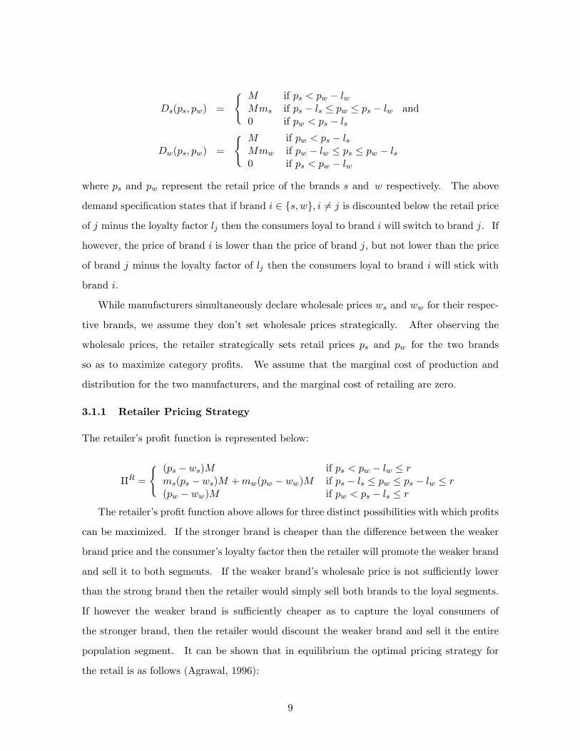
Ds(ps; pw) =

( M if ps < pw � lwMms if ps � ls � pw � ps � lw0 if pw < ps � ls

and

Dw(ps; pw) =

( M if pw < ps � lsMmw if pw � lw � ps � pw � ls0 if ps < pw � lw

where ps and pw represent the retail price of the brands s and w respectively. The above

demand speci�cation states that if brand i 2 fs; wg; i 6= j is discounted below the retail price

of j minus the loyalty factor lj then the consumers loyal to brand i will switch to brand j. If

however, the price of brand i is lower than the price of brand j, but not lower than the price

of brand j minus the loyalty factor of lj then the consumers loyal to brand i will stick with

brand i.

While manufacturers simultaneously declare wholesale prices ws and ww for their respec-

tive brands, we assume they don�t set wholesale prices strategically. After observing the

wholesale prices, the retailer strategically sets retail prices ps and pw for the two brands

so as to maximize category pro�ts. We assume that the marginal cost of production and

distribution for the two manufacturers, and the marginal cost of retailing are zero.

3.1.1 Retailer Pricing Strategy

The retailer�s pro�t function is represented below:

�R =

( (ps � ws)M if ps < pw � lw � rms(ps � ws)M +mw(pw � ww)M if ps � ls � pw � ps � lw � r(pw � ww)M if pw < ps � ls � r

The retailer�s pro�t function above allows for three distinct possibilities with which pro�ts

can be maximized. If the stronger brand is cheaper than the di¤erence between the weaker

brand price and the consumer�s loyalty factor then the retailer will promote the weaker brand

and sell it to both segments. If the weaker brand�s wholesale price is not su¢ ciently lower

than the strong brand then the retailer would simply sell both brands to the loyal segments.

If however the weaker brand is su¢ ciently cheaper as to capture the loyal consumers of

the stronger brand, then the retailer would discount the weaker brand and sell it the entire

population segment. It can be shown that in equilibrium the optimal pricing strategy for

the retail is as follows (Agrawal, 1996):

9

� if ww > ws + (1=mw)lw then charge ps = r � lw � �; pw = r;

� if ws + (1=mw)lw � ww � ws + (1=mw)lw then charge ps = r and pw = r ; and �nally

� if ws > ww + (1=ms)ls then charge pw = r � ls � �; ps = r.

It is important to note that the retailer is maximizing pro�ts for the overall category.

As a result they always have the option to sell both brands at the reservation price to the

corresponding loyal segments of the market. The retailer only discounts one of the brands if

the wholesale price o¤ered for that brand is low enough to warrant a higher pro�t by selling

the one brand at a discounted rate to the entire market.

This equilibrium pricing strategy leads to several hypotheses about the frequency and

depth of discounts o¤ered by a retailer. First, deeper discounts are given by the retailer for

the weaker brand in comparison to the stronger brand. This this result follows directly from

the optimal pricing strategy above because the weaker brand has to o¤er a larger discount ls

in order to attract the stronger brand�s loyal customers and 0 < lw � ls. In other words,

� H1: the average price discount at the retail level is negatively related to the strength

of brand loyalty.

In equilibrium the retailer promotes the stronger brand with a probability: Pr[ww >

ws + (1=mw)lw], and promotes the weaker brand with probability: Pr[ws > ww + (1=ms)ls]:

Given the asymmetry in loyalties (lw � m2wr and ls � ms(r � lw)(1 + msmw)

�1) (Raju,

Srinivasan, and Lal, 1990) it follows that the probability of the weaker brand obtaining the

consumers loyal to the stronger brand is zero, which suggests that the retailer will promote

the stronger brand more frequently. In other words,

� H2: the frequency of price promotions at the retail level is positively related to the

strength of brand loyalty.

Since these hypotheses follow directly from the model described above, their support or

rejection will give valuable insight into the underlying assumptions of our theoretical model.

For example H1 will be able to shed light on the validity of the underlying assumption of the

measure of brand loyalty. If H1 is rejected then our de�nition and distinction of the stronger

or weaker brand would be fundamentally �awed and our operationalization of brand loyalty

10

should be reconsidered. Similarly, rejection of H2 may indicate that retailers use promotions

strategically to compete with other retailers even at the product level as suggested by Lal and

Villas-Boas (1998). In the section that follows we develop an empirical model of consumer

demand that provides household-level estimates of brand preference. These estimates will

then be used to test H1 and H2:

4 Empirical Model of Brand Loyalty

In this section we develop an empirical model of brand loyalty designed to test the hypothe-

ses above. We estimate brand loyalty using a discrete choice approach, as opposed to a

representative consumer demand model. Representative consumer demand models assume

a consumer is, on the whole, average, and thus consumes a small amount of every brand in

the category (Anderson, de Palma and Thisse, 1992). By assuming that the market consists

of millions of representative, utility maximizing consumers, representative consumer demand

models try to explain how demand is likely to change if prices, income, or some other depen-

dent variable changes on the assumption that everyone is alike and has the same preferences.

Examples of representative consumer demand models include the Constant Elasticity of Sub-

stitution (CES) (Dixit and Stiglitz, 1977), and the Almost Ideal Demand System (AIDS)

(Deaton and Muellbauer, 1980).

Representative consumer models, however, are generally written as systems of demand

equations, in which the interrelated nature of consumer demand is explicitly recognized. A

systems approach to demand estimation provides consistently better empirical results that

are more consistent with the underlying theory of constrained utility maximization elemen-

tary economic theory than single-equation alternatives. But, in a di¤erentiated-product

environment, the assumption that consumers buy every product is not tenable. Rather,

when brands are di¤erentiated, consumers prefer di¤erent brands given they perceive prod-

uct attributes di¤erently. Representative consumer demand models do not take into account

this consumer heterogeneity.

As an alternative to representative consumer demand models, Luce (1959) and McFadden

(1973) developed the logic that underlies discrete choice models. In a discrete choice frame-

work, consumers are assumed to buy the one brand that yields the greatest utility over all

other choices. Utility, however, is randomly distributed and depends upon the distribution

11

of unobserved consumer preferences, or unobserved heterogeneity. By specifying a functional

form for the unobserved consumer heterogeneity, discrete choice models are able to more read-

ily capture why consumers buy particular brands. However, the parameters in the utility

function are assumed to be constant over consumers in the simple logit speci�cation. This

assumption is convenient as a closed form demand equations results. Nonetheless, the simple

logit is subject to the independence of irrelevant alternatives (IIA) property, which means

that substitution patterns are based on market share instead of fundamental attributes of

the brand. In order to fully accommodate household heterogeneity we allow the parameters

to vary randomly, which causes substitution between brands to be based on brand attributes

instead of market share. This speci�cation is not without cost, as the mixed logit no longer

yields a closed form demand equation. However, estimation of the closed form demand

equation is not necessary to empirically estimate the strength of loyalty for each product, nor

the size of the loyal segment. We describe the speci�c model we use for this purpose in the

next section.

4.1 Consumer Demand

Breakfast cereals are highly di¤erentiated food products. Consequently, we model their

demand using a discrete choice approach (Anderson, de Palma and Thisse, 1992; Jain, Vil-

cassim, and Chintagunta 1994; Nevo, 2001). Of all possible discrete choice models, we model

consumer demand with a random coe¢ cient logit model (RCL). Compared to the simple, and

nested logit forms, the RCL has several advantages. First, the partial derivatives of the brand

choice probability will not be determined by a single parameter as in the logit and nested logit

models. Instead, each household in the sample will have a di¤erent price sensitivity, which

is important to the objectives of this study. Namely, the price response parameter di¤ers

among brands, which provides an appropriate measure of the brand�s strength. Second, the

RCL model allows for �exible substitution patterns, unlike the simple and nested alternatives

(within nests). Consumer heterogeneity is allowed to enter the model through a composite

random shock term that is dependent on product and individual characteristics. Thus, if

the price of a brand goes up, households are more likely to switch to a brand with similar

characteristics, as opposed to the one that, on average, is most often purchased. Third,

and because of this feature, households with similar characteristics will tend to have similar

12

purchasing patterns.

Formally, we assume that a sample of H households h 2 f1; 2; :::;Hg make a purchase

among N brands b 2 f1; 2; :::; Ng on purchasing occasion t 2 f1; :::; Tg. Then the conditional

indirect utility of household h for alternative b on purchasing occasion t can be written as:

uhbt = hb + �0xhbt � �hbphbt + �hbt + �hbt (1)

where �hbt is an error term that accounts for all product-speci�c variations in demand that are

unobserved by the econometrician.2Brand b�s price is represented by phbt, and hb captures

the intrinsic preference of household h for brand b, � is a k-dimensional vector of parameters

and xhbt is a vector of attributes of the household and the brand, which includes variables

such as household income, an indicator of whether the product is o¤ered on a temporary

discount (dcbt), and an interaction term between the retail price and the discount (dcbtpbt)

(Chintagunta, 2002; Richards, 2006). By including an interaction term we allow for the

possibility that promotion rotates the demand curve in addition to the expected demand-

shifting e¤ect. In this way, we allow items on promotion to become less elastic if households

perceive discounting as a means of di¤erentiating otherwise similar products. These ex-

planatory variables, and their distribution over households, govern the substitution patterns

so that products with similar characteristics will be closer substitutes. Furthermore, we

assume that the error term �hbt is an i.i.d. type I extreme value error term that accounts

for household-speci�c heterogeneity in preferences. With this error assumption, the utility

speci�cation in (1) implies a discrete choice logit demand model.

It is well understood that a simple logit model su¤ers from the IIA property. The

RCL model does not have this attribute because the correlation between random parameter

variation and attributes included in the demand model introduces a degree of curvature that

the simple logit lacks. In the RCL, we allow the product-preference and marginal utility of

income parameters in (1) to vary over consumers in a random way (BLP, 1995; Nevo, 2001).

Speci�cally, the marginal utility of income is normally distributed over households such that:

�hb = �+ ���hb; �hb s N(0; 1) (2)

2Because we use t to denote the time period and T to denote the total number of time periods we use a�0�, instead of the traditional poscript T, to denote the transpose of a vector or matrix.

13

where � is the mean price response across all consumers and �hb is the household-speci�c

variation in response with parameter ��. We can decompose �0into f�1; :::; �L; �L+1:::; �kg

where the �rst L parameters are the random parameters, and the L + 1 parameters rep-

resent the non random parameters, such as the discount indicator and discount interaction

term. We decompose xhbt in a similar way. Households, therefore, are assumed to di¤er in

their attribute preferences such that unobserved consumer heterogeneity is re�ected in the

distribution of each brand�s marginal utility in the following way:

�hl = �l + ��zhl + ��vhl; vhl s N(0; 1) l = 1; :::; L: (3)

where �l represents the �xed constant terms in the means of the distributions for the random

parameters, zhl represents a set of observed variables which do not vary over time and enter

the means of the random parameters, �� is the set of coe¢ cients that form the observation

speci�c term in the mean, vhl is the random term representing the household�s unobserved

heterogeneity and �� is the coe¢ cient of the household�s unobserved heterogeneity. McFad-

den and Train (2000) interpret the elements of (3) in terms of an error-components model of

attribute demand. In contrast to the IIA property of a single logit model, the heterogeneity

assumption in (3) creates a general pattern of substitution over N alternatives through the

unobserved, random part of the utility function given in (1). As a result, the utility from

di¤erent brands is correlated according to the set of attributes included in xhbt.

The mixed logit model introduces a large number of parameters relative to the simple

logit model. Therefore, we follow Nevo (2001), among others, and write the indirect utility

function in terms of two sets of variables - those that are assumed to be random and those

that are not:

uhbt = �hbt(phbt;xhbt; �hbt; hb; �hb;�hl) + �hbt(phbt; �hb; vhl;��; ��; ��) + �hbt (4)

where �hbt is the mean utility level that varies over products, but not households, and �hbt

is the idiosyncratic part that varies by household and product. For convenience let �hbt =

hb+�0xhbt��hbphbt+ �hbt: With this, the probability that household h chooses brand b at

purchasing occasion t conditional on �hl, and �hb can be written:

14

Prht(b j �hl; �hb) =

TYt=1

e�hbt

1 +PN�1i=b e

�hbt: (5)

where the utility of purchasing brand N has been normalized out.

The advantages of the RCL model do not come without a cost. Unlike the logit and nested

logit models, there is no analytical closed form for (5). In order to overcome this di¢ culty,

we integrate over the densities of the random parameters in the model. De�ne the densities

of fvh1; :::; vhLg as ff(vh1); :::; f(vhL)g and �h as g(�h) so that the unconditional probability

of household h purchasing brand b on purchasing occasion t is obtained by integrating over

(5) and the distributions re�ecting consumer heterogeneity. Doing so we obtain:

Prht(b) =

Z:::

Z TYt=1

e�hbt

1 +PN�1i=b e

�hbtf(vh1):::f(vhL)g(�h)dvh1:::dvhLd�h (6)

which can then be estimated using simulated maximum likelihood.

4.2 Measure of Brand Strength

Our study of brand loyalty de�nes brand loyalty as the price di¤erential needed to make a

consumer who prefers one brand switch to a less preferred brand (Pessemier, 1959). Conve-

niently, this measure of brand loyalty is captured by the product-preference term (constant)

in the RCL speci�cation described above. By estimating the RCL over purchase occasion,

time, and household we are able to recover unbiased estimates of each household�s preference

for each brand. Therefore, we use each household�s preference ( hb) as a measure of brand

strength (Agrawal, 1996). We obtain the measure of brand strength for brand b by taking the

average over every household�s preference for that brand which we�ll denote b. In this way,

our measure of brand strength, b, is able to capture the attitudinal and behavioral aspects

of brand loyalty described above. Furthermore, we use this measure of brand strength to de-

termine the number of consumers who prefer that brand, or the brand�s "size." Our method

di¤ers from that of Agrawal (1996) in that our brand strength is estimated for household

h and brand b which provides a richer set of data with which to estimate the relationship

between brand strength and retailer�s promotional strategies. Furthermore, our estimates of

brand strength are computationally easier compared to the semiparametric alternatives he

uses, while still accounting for household speci�c heterogeneity. Consequently, our method

15

guarantees strength and size estimates for each brand in the category, which is essential for

testing the hypotheses of the theoretical brand loyalty model.

A precondition to explaining the frequency and depth of retail price promotions as they

relate to brand loyalty is that brand loyalty indeed exists within the category (Huang, Perlo¤,

and Villas-Boas, 2006). If the households within our sample have no preference for one brand

over another then our empirical tests of H1 and H2 cannot be carried out. As a result, our

�rst hypothesis test will be

� H0: no brand loyalty exists among the brands.

Since b measures the average strength of brand b it follows that if b = 0 8b then

our model would suggest no brand loyalty exists among the brands, because on average the

household wouldn�t prefer any one brand over another. If we fail to reject H0; then the model

wouldn�t be suitable to test hypotheses H1 and H2. If we reject H0 then we can empirically

explain the frequency and depth of retail price promotions as they relate to brand strength.

In order to estimate the relationship between brand strength and price promotions, we

specify a second-stage regression model in which the retailer�s promotion strategy is a function

of brand strength. De�ning the discount o¤ered by a retailer as the percentage change in

prices from one week to the next, we use the actual percentage decrease as a measure of the

depth of the retail promotion. If we regress brand b�s strength on the measure of promotion

depth, we are able to test the central hypothesis of the study, namely that the average price

discount at the retail level is negatively related to the strength of brand loyalty. Therefore,

the estimated model becomes:

dbt = �d0 + �d1prefb + �d2sizeb (7)

where prefb is the strength of brand b; dbt is the depth of the discount o¤ered on brand b at

week t; sizeb is the percentage of households who prefer brand b; and �d0 is the intercept of

the model that accounts for the depth of the discount when brand strength and size aren�t

present.3 This speci�cation allows us to test H1, namely, if �d1 > 0 then the depth of the

price discount at the retail level is negatively related to the strength of brand loyalty. Since

3Recall that we expanded the choice set to include all possible combinations of purchases within thecategory. For this stage of the model we will only use the actual brand estimates and not the expanded choiceobservations since they are aggregates of the other brands.

16

the discount is negative by de�nition, and brand strength is positive, it follows that �d1 > 0

implies an inverse, or negative, relationship. If however, �d1 < 0 then we would reject H1.

Furthermore, this speci�cation will allow us to investigate the relationship of the brand�s

marketshare and the depth of the retail discount.

We develop a similar test for the frequency of price promotions. We de�ne promotion

frequency as the average number of times the brand is discounted at least 10% from one day to

the next each week. Similar to the approach described above, we then regress the strength

and size of each brand on the measure of promotional frequency. We model frequency

promotion as follows:

fbt = �f0 + �f1prefb + �f2sizeb (8)

where fbt is the promotional frequency for brand b during week t; prefb and sizeb are again

the strength and size of brand b, and �f0 is the intercept of the model that accounts for

the frequency of the discount when brand strength and size aren�t present. Estimating this

model allows us to test H2. More speci�cally, if �f1 > 0 then the frequency of retail price

promotions is positively related to the strength of brand loyalty. Because fbt; and prefb are

positive values, a positive coe¢ cient estimate suggests that frequency rises as the strength

of loyalty rises. This positive relationship comes from the asymmetry in loyalties derived by

Raju, Srinivasan, and Lal, (1990), namely that lw � m2wr and ls � ms(r� lw)(1+msmw)

�1.

From this it follows that the probability of the weaker brand obtaining the consumers loyal to

the stronger brand is zero, which suggests that the retailer will promote the stronger brand

more frequently. If, on the other hand, we �nd that �f1 � 0 then we reject H2 and conclude

that this asymmetry doesn�t hold in the RTE cereal industry. If H1 and H2 are supported

then our empirical �ndings provide evidence that the theoretical model developed above is

representative of the RTE cereal category and may serve as a basis for other theoretical

derivations of brand loyalty. A summary of our tests for the frequency and depth of retail

price promotions is as follows:

� H0: No brand loyalty exists among any of the brands. ( b = 0 8b)

� H1: The average price discount at the retail level is negatively related to the strength

of brand loyalty. (�d1 > 0)

17

� H2: The frequency of price promotions at the retail level is positively related to the

strength of brand loyalty. (�f1 > 0)

5 Estimation Method

In this section we explore the estimation method used to estimate the above models. Fol-

lowing Agrawal (1996) we estimate (7) and (8) using Joint Generalized Least Squares (SUR)

estimation technique, which results in more e¢ cient, though identical, estimates compared

to OLS estimation. The SUR takes into account the correlation in error terms across the

equations. There are several complications to address when estimating equation (6) above.

First, the unobserved factors are correlated over time within each household. Maximum

likelihood estimates will provide consistent estimates of the endogeneity of the households

unobserved factors by allowing the coe¢ cients on the decision to vary randomly. Second,

the probability equation cannot be estimated using ordinary least squares because there is

no closed form for the equation. Simulated maximum likelihood uses Monte Carlo simula-

tion to solve the integral in (6) up to an approximation that is accurate to the number of

random draws chosen, R: Finally, some of the unobserved factors may be correlated with

the explanatory variables. As a result the demand model is estimated using the method of

simulated maximum likelihood. This method provides consistent parameter estimates under

general error assumptions and is readily able to accommodate complex structures regarding

household heterogeneity. As models of this form can be quite computationally burdensome

we implore a Halton draw sequence. This sequence signi�cantly cuts down on the number of

draws with no degradation to simulation performance (Bhat, 2003). We found that R = 200

draws are su¢ cient to produce stable estimates without excessive estimation time.

6 Data Description

In this section we describe the data used for the econometric model developed in section

4. The empirical estimation requires data on prices, product characteristics, and household

demographics. Wind and Lerner (1979) �nd that self-reported survey data is often unreliable

as it is dependent on the recalling of purchase events from memory. Consequently this study

uses a household panel data gathered by A.C. Nielson. A.C. Nielson, Inc.�s "HomeScan"

data has participating households submit all food purchase information (price, quantity,

18

along with a product description) each time they visit any type of retail food outlet. The

homescan database also includes a number of socioeconomic and demographic descriptors.

We use all shopping trips from the beginning of 2006 to the end of 2006. This time period

is long enough to observe several category purchases, while short enough to assume the

household�s preferences haven�t changed over time. Using such a detailed household sample

should provide su¢ cient empirical data to determine how a household�s brand loyalty a¤ects

a retailer�s equilibrium promotional strategy for di¤erentiated products.

As mentioned above the RTE cereal industry �ts well with the purposes of this study

due to the high frequency of purchase, and �erce brand rivalry. We randomly select 1020

households who made at least two purchase within the RTE cereal industry. Selecting the

households at random from the homescan data should give us a representative sample of

US consumer buying habits. In table 2 we present the demographic information from the

Current Population Survey (CPS) for 2006 and compare it to the surveyed households of the

A.C. Nielson Homescan data. We can see from table 2 that the demographics of the A.C.

Nielson households match those of U.S. households quite well. As a result, we suggest that

our randomly sampled population is a representative sample of U.S. households

Insert Demographic Table Here

The variety of brands available in the RTE cereal industry poses a bit of a problem

because product speci�c attributes must be available on every brand the household might

consider purchasing. As a result, we select only those brands within the RTE industry with

the highest marketshare. By selecting the most popular brands in the category we increase

the probability a randomly selected household made a purchase. We �ll in the information

on brands the household didn�t purchase using purchases made by other households in the

same geographic area, the same day, and if the same day isn�t available, the same week.

By selecting the most popular brands we increase the richness of the information on choices

not selected by the household. The brands selected were General Mills�Cheerios, Kelloggs�

Frosted Mini-Wheats, General Mills�Honey Nut Cheerios, Post�s Honey Bunches of Oats,

Kelloggs�Frosted Flakes, and General Mills�Cinnamon Toast Crunch. These brands tend

to have the highest marketshare of all brands, which results in high incidences of purchase.

Summary statistic on the brands used in the dataset can be found in table 3, including how

19

often the brands were purchased by the households throughout 2006 and the prices of each

brand (in cents per ounce).

Insert RTE summary stats. Table Here

6.1 Multiple Discreteness

It is well known that the choice set of discrete choice models must exhibit alternatives which

are mutually exclusive from the decision maker�s perspective (Train, 2003). In other words,

choosing one alternative necessarily means another cannot be chosen. For many of the

product categories found in retail grocery outlets consumers regularly purchase assortments

of products and di¤erent brands within the product categories. The marketing literature

provides several explanations as to the reason consumers might make several purchases within

a particular category. McAlister (1982) found that consumers seek variety over time and

in so doing switch their consumption of several di¤erent �avors. Consequently this form of

variety seeking would induce a consumer to select an assortment of alternatives. Similarly,

if households are unsure of their future tastes at the time of consumption they may purchase

an assortment to ensure they have the right variety on hand (Hauser and Wernerfelt, 1990;

Simonson, 1990; and Walsh, 1995). This could be particularly true if the household has

several members and the purchasing member of the household is unsure of the other member�s

tastes.

This multiple discreteness violates the mutual exclusivity assumption of discrete choice

models. This misspeci�cation would produce incorrect measures of consumer response to

marketing mix variables. Recognizing the di¤erence between the time of purchase and the

time of consumption, Dube (2005) accounts for multiple discreteness by modeling the number

of consumption occasions the household faces during each shopping trip. Thereby suggesting

that only one product is being consumed at a particular time. In this way they are able

to develop a "vertical" variety-seeking model that accounts for multiple discreteness within

category purchases. Hendel (1999) models the di¤erent tasks the consumer is going to use

the di¤erent brands for. In so doing he is able to account for multiple discreteness within

a RCL model. Bhat (2005) proposes a simple, parsimonious model to account for other

choice occasions such as time allocation to di¤erent types of discretionary activities. He

describes the decision process as "horizontal" variety-seeking, where the consumer selects an

20

assortment of alternatives due to diminishing marginal returns for each alternative. In so

doing Dube (2005) and Bhat (2004) are able to take into account total demand elasticities.

The theoretical structure requirements proposed by Hendel (1999), Dube (2005), and Bhat

(2005) impose too many restrictions on the underlying utility model to be entirely useful for

our case. As a result we follow Train, McFadden, and Ben-Akiva, (1987) and expand the

choice set such that each possible portfolio of choices is a distinct alternative.4 Expanding the

choice set essentially ignores the complementarity between the two products being purchased

since buying two together is fundamentally di¤erent from buying one and then the other.

Since we are trying to identify the degree of brand loyalty for each product, we don�t need to

consider total demand elasticities. As we can see in table 3 the real gain from expanding the

choice set doesn�t come from the measure on the newly introduced choices, but rather from

the increasing number of households and their corresponding brand purchases. For example,

if a household bought Cheerios every time and once bought Cheerios and something else, their

observations couldn�t be used in our discrete choice model. Whereas now we can include

those observations. Furthermore, this is still consistent with utility maximization because

we�re looking at households, the overall utility of the household is greater when buying two

products together, as opposed to only one. Within the dataset if we had restricted the data

to be only those households who purchased a single brand each trip we would have used 877

households (N = 26; 904). By expanding the choice set to include households that made

at least one purchase within the category, we are able to observe the purchasing habits of

1020 households in total (N = 76; 024). By increasing the number of choices from 6 brands

to 13 we have 5848 observations per choice. As a result, expanding the choice set allows

us to include those households that make more than one brand purchase, adding valuable

information to the analysis.

7 Empirical Results and Discussion

In this section, we present the results obtained from estimating the three equations that

comprise the strategic price-promotion model as it pertains to brand loyalty and draw several

implications for the further study. We �rst present and discuss the demand-system estimates

4 In fact we only had to expand the choice set by those combinations of brands that were actually purchased,which was sign�cantly less than all the possible combinations.

21

that empirically determine the level of preference each household has for each brand. With

estimates of brand strength we �rst test H0 that states there is no brand strength among

the products, and if rejected, we�ll proceed to test the other hypotheses. Using the demand

estimates we calculate the e¤ect brand loyalty has on the depth and breadth of retailer

promotions. In so doing we�ll look at the hypothesis that the average price discount at the

retail level is negatively related to the strength of brand loyalty (H1) and the hypothesis that

the frequency of price promotions at the retail level is positively related to the strength of

brand loyalty (H2).

As a �rst step to interpreting the demand model results we test the validity of the RCL

model in general, and against the simpler logit speci�cation as discussed in the estimation

section. Several tests exist that allow us to investigate how well the model �t the data and

whether or not a RCL speci�cation is preferred over the simpler multinomial logit form in

which the parameters are �xed. The likelihood ratio index is often used with discrete choice

models to measure how well the model �t the data. If the estimated model is not any better

than no model at all the we�ll �nd that likelihood ratio index is very close to zero. We

�nd that the log-likelihood ratio index for the RCL model is 0:49 which means that our RCL

model �ts the data better than a model containing no parameters: Furthermore in comparing

the log-likelihood ratio index against the simpler logit model we �nd that the simpler model

has a likelihood ratio index of 0:02 which implies that, given the same parameters and data,

the RCL model �ts the data better than the simple logit model. The main di¤erence between

the two models is their ability to handle household heterogeneity. If no heterogeneity exists

in the model then the coe¢ cients ��; ��; and �� will all equal zero and the RCL will collapse

into the simple logit model. As we can see in table 4 several of the coe¢ cients are statistically

di¤erent from zero. Consistent with Jain, Vilcassim, and Chintagunta (1994) this suggests

that heterogeneity exists in the data and not accounting for it would provide biased estimates

of brand strength. Therefore we conclude that the RCL model �ts that data better than the

simple logit model and we will use these estimates to interpret household demand.

In the demand model, the parameters of interest are the own-price e¤ect, the discount-

e¤ect, the discount-price interaction term, and the average intrinsic preference for brand b.

The own-price e¤ect, measured by the marginal utility of income, is negative as expected.

Consistent with the theoretical model this suggests that the households will have some reser-

22

vation price r, at which they will no longer make a purchase. We obtain the estimate of the

marginal utility of income by averaging each household�s estimate. In table 4 we can see

that the coe¢ cients on both the discount-e¤ect, and the discount-price interaction term are

not statistically signi�cant. Within the context of the model this implies that discounting

doesn�t have a signi�cant a¤ect on which brand the household purchases. We�ll now pro-

ceed to test H0 which states that no brand strength exists among the brands ( b = 0 8b).

The results in table 4 show that several of the brands are statistically di¤erent from zero,

which suggests that on average, households have some preference for one brand over another.

We therefore reject H0 and conclude that the households used for the sample exhibit brand

loyalty.

Insert Demand Results Table Here

The parameter estimates in table 4 provide valuable information on the RTE cereal in-

dustry. Recall from section 4 we normalized brand N out. As a result our estimates in

table 4 are the average brand preference for brand b relative to brand N: In our case brand

N happens to be the option of purchasing both Honey Bunches of Oats, and Cheerios in one

shopping trip. From table 4 we can see Cheerios is the most preferred brand, which would

be expected given it has the highest marketshare of any RTE cereal brand. Honey Bunches

of Oats is the second highest preferred brand, and we �nd that the choice of purchasing both

Honey Bunches of Oats and Cheerios is the preferred choice over any other choice combina-

tions, which is consistent with the model�s overall results. Furthermore, it seems that on

average, households prefer to choose one brand at a time with the exception of Cinnamon

Toast Crunch. Given the overall signi�cance of the brand preference estimates, we can use

these to estimate the strength of each brand and test H1 and H2.

Using the estimates from the RCL model we calculate each household�s preference for

brand b: The results of the Joint Generalized Least Squares estimates of the discount model

are presented in table 5. We�ll �rst look at the overall �t of the model to the data. We �nd

that the R2 is 0:059 which indicates that the brand strength and size only account for 5.9%

of the depth of the retailer discount. We can test the overall signi�cance of the model using

a F-test. We see in table 5 that the model�s F-statistic is 4:50. The corresponding test

statistic at the 95% level of signi�cance is 3:025 given a numerator of 2, and a denominator

23

of 310. Since our F-statistic is greater than 3:025 we can reject the null hypothesis that all

of the parameters are equal to zero. Given the signi�cance of the model overall we�ll use

these estimation results to test H1.

Insert Discount Regression Table Here

The primary parameters of interest in table 5 are �d1, and �d2. If �d1 > 0 then the depth

of the price discount at the retail level is negatively related to the household�s preference

of brand b: From the discount model estimates we can see that �d1 > 0 and statistically

signi�cant at the 95% level of signi�cance. As a result the estimate of �d1 provides evidence

for H1, namely that the depth of the price discount at the retail level is negatively related to

the strength of the brand preference. This suggests that the weaker brand will be promoted

deeper than a stronger brand which provides evidence towards the promotional equilibrium

of our theoretical model. This also provides evidence for the measurement of brand loyalty.

Note that if H1 were rejected it would suggest that the stronger brand would be promoted

deeper than the weaker in order to attract the loyal customers of the weaker. This would

fundamentally contradict our de�nition and distinction of the stronger and weaker brands.

As a result, by not rejecting H1 we provide evidence of Pessemiers�(1959) de�nition of brand

loyalty and conclude that it is a reasonable assumption for the RTE cereal industry. Further-

more, it provides evidence to suggest that the duopoly model may extend to a multiproduct

market. From table 5 we also see that the e¤ect the size of the loyal cohort has on the depth

of the discount is insigni�cant. Since �d2 is not statistically di¤erent from zero it follows

that the size of brand b�s loyal cohort doesn�t have a signi�cant e¤ect on the depth of its

promotion. We test our model further by investigating the relationship of brand strength

and promotional frequency.

The demand estimates shown in table 4 form the key inputs to the second-stage promo-

tional frequency model estimates shown in table 6. The results of the Joint Generalized Least

Squares estimates of the frequency model are presented in table 6. While looking at the �t

of the model to the data we �nd that the R2 is only 0:02, which indicates that the brand�s

strength and size account for very little in the variation of the promotional frequency. We

can test the overall signi�cance of the model using the F-statistic which we can see is 4:01.

The corresponding test statistic at the 95% level of signi�cance is 3:025 given a numerator

24

of 2 and a denominator of 310. Since our F-statistic is greater than 3:025 we can reject the

null hypothesis that all of the parameters are equal to zero and proceed to test H2.

Insert Frequency Regression Table Here

In table 6 the primary parameters of interest are �f1; and �f2 which measure the e¤ect

the brand�s strength and marketshare (size) has on the frequency of promotion. If �f1 > 0

then the frequency of price promotions at the retail level is positively related to the strength

of brand loyalty. The results in table 6 indicate that �f1 < 0 and statistically signi�cant at

the 95% level of signi�cance. As a result we reject H2 and conclude that the frequency of

price promotions at the retail level is negatively related to the strength of brand loyalty. This

is in contrast to our theoretical model developed in the 3rd section. Within the theoretical

model�s context this would suggest that the weaker brands are promoted more frequently

than the stronger brand. This suggests that the probability of the weaker brand obtaining

the loyal consumers of the stronger brand is not zero. Thus the asymmetry of loyalties derived

by Raju, Srinivasan, and Lal�s (1990) model does not hold within the RTE cereal category.

Furthermore, we see from table 6 that the estimate of the brand�s size is not statistically

di¤erent from zero. This would suggest that the marketshare of a brand is not an indicator

of the depth or frequency a brand will be promoted at the retail level.

Our result suggest that there is a high degree of brand loyalty within the RTE cereal

industry and the data does not fully support the patterns suggested by our theoretical model.

By rejecting H2 we conclude that the theoretical model developed above is not a representative

model of brand loyalty in the RTE cereal category. However, our empirical results do con�rm

those of Agrawal (1996) and suggest that the promotional depth of a retailer�s discount is

negatively related to the strength of brand loyalty. In other words, deeper discounts are

given for weaker brands if the wholesale price o¤ered for that brand is low enough to warrant

a higher pro�t by selling the weaker at the discounted rate to the entire market. This

empirical result supports our de�nition, and distinction between the stronger and weaker

brands, namely that lw � ls. Furthermore, our empirical results suggest that the brand�s

marketshare is insigni�cant in determining the depth and breadth of retail promotions.

Our results also suggest that the weaker brands are promoted more frequently than the

stronger brands. In other words, the frequency of price promotions at the retail level is

25

negatively related to the strength of the brand. This suggests that the asymmetry of our

theoretical model�s loyalties, namely that lw � m2wr and ls � ms(r � lw)(1 + msmw)

�1

as shown by Raju, Srinivasan, and Lal, (1990), does not hold for the RTE cereal category

because the weaker brand is able to capture the marketshare of the stronger brand with a

probability greater than zero. Otherwise the retailer would promote the stronger brand more

frequently. Therefore it follows that this assumption is not suitable for brand loyalty models

in the RTE cereal category and should be reconsidered in further research.

8 Conclusion and Implications

Though brand loyalty has been studied extensively in the marketing literature, the rela-

tionship between brand loyalty and equilibrium pricing strategies is not well understood.

Retailer�s promotional decisions are critically dependent upon how many consumers can be

convinced to switch to a brand by temporarily reducing its price, and how many are in-

stead brand loyal. Theoretical models of how the size and strength of brand loyalty in�uence

optimal promotion strategies have been developed, but there are no rigorous tests of their

hypotheses. As a result we empirically determine how brand loyalty changes retailer�s equi-

librium promotional strategy for di¤erentiated products.

We develop and test a theoretical model of brand loyalty that resembles many of the

fundamental characteristics of theoretical brand loyalty studies. In our empirical estimation

we use a random coe¢ cient logit model to estimate the intrinsic preference each household

has for each brand. Estimating the random coe¢ cient logit model using simulated maximum

likelihood provides consistent estimates of the mean household preference while accounting

for the heterogeneity among households. Using household panel data we applied the em-

pirical test to the purchases made by the households throughout the US during 2006. By

applying our random coe¢ cient logit model to this rich panel data we were able to empirically

investigate retail promotion strategies.

The result suggest that there is a high degree of brand loyalty within the RTE cereal

category and the data does not fully support the patterns suggested by our theoretical model.

We conclude that the theoretical model developed above is not a representative model of

brand loyalty in the RTE cereal category. Our results suggest that the average price discount

at the retail level is negatively related to the strength of brand loyalty as implied by the

26

theoretical model. In other words, deeper discounts are given for weaker brands if the

wholesale price o¤ered for that brand is low enough to warrant a higher pro�t by selling

the weaker at the discounted rate to the entire market. These empirical result supports our

de�nition, and distinction between the stronger and weaker brands. However, contrary to the

maintained hypothesis of many studies in retailing our results also suggest that the weaker

brands are promoted more frequently than the stronger brand. In other words, the frequency

of price promotions at the retail level is negatively related to the strength of the brand. It

therefore follows that assumptions of theoretical brand loyalty models that concluded that

the frequency of price promotions at the retail level is positively related to the strength of

the brand should be reconsidered in future research when being applied to the RTE cereal

category.

Though our results have implications for future work with models of retail price pro-

motion, there is much that remains for the study of both theoretical and empirical models.

Future empirical research would bene�t by empirically studying the e¤ect a price sensitive

segment would have on the retailer�s promotional strategies. The size of a price sensitive

segment may provide insight into the degree of brand loyalty within the market and the

overall incentives of a retailer and their potential strategic interaction within that market.

Future research would also bene�t by considering, empirically, the e¤ect trade deals have

on a promotional equilibrium. Our empirical model wasn�t able to estimate the retail pass

through and trade deals as a result of the household speci�c data. However, methods have

been proposed that a suggest ways to estimate the trade deals given to retailers.5 Incorpo-

rating this into empirical studies of brand loyalty would reveal valuable information on the

retailer�s strategic interaction within the market and their overall incentive to o¤er a price

promotion. The empirical evidence from such a study would be able to distinguish between

a retailer�s incentive of a larger margin, and the competitive nature of the market in general.

Future theoretical research in the study of retailer promotional strategies may bene�t by

investigating the theoretical rami�cations of a market that consists of more than two brands.

Since most retail markets inherently have more than two products the applications certainly

exist. In so doing one could investigate the possibility of complementary products and their

e¤ect on retailers promotional decisions in the marketplace. Future theoretical research may

5This includes Richards, Pofahl, and Hamilton (2007).

27

also bene�t from looking at the dynamic long run game theoretic aspects of promotional

strategies. This would allow models to relax the assumption that the manufacturer sets

prices simultaneously, and assume a sequential price setting. This would be a more realistic

assumption and would allow theoretical applications to investigate the e¤ect trade deals

would have on the opposing manufacturer and the resulting equilibrium. Lastly, it would

also be reasonable to assume that manufacturers are aware of the wholesale price of several

products within the market. Since many highly concentrated industries have only a few

manufacturers selling multiple products it follows that they would know the wholesale price

of some portion of the products within the market. This would allow researchers to model

the possibility that a manufacturer to promote several of their own brands at the same in

order to attract the marketshare away from a competing brand.

28

References

[1] Agrawal, Deepak. �E¤ect of Brand Loyalty on Advertising and Trade Promotions: A

Game Theoretic Analysis with Empirical Evidence�Marketing Science 15 (1996): 86-

108.

[2] Anderson, Simon P., Andre de Palma, and Jacques-Francois Thisse. Discrete Choice

Theory of Product Di¤erentiation. Cambridge: MIT Press, 1992.

[3] Assunção, João. L., and Robert J. Meyer. "The Rational E¤ect of Price Promotions on

Sales and Consumption" Management Science 39 (1993): 517-535.

[4] Barten, A. P. "Maximum Likelihood Estimation of a Complete System of Demand Equa-

tions" European Economic Review 1 (1969):7-73.

[5] Besanko, David, Jean-Pierre Dube, and Sachin Gupta. "Competitive Price Discrimina-

tion Strategies in a Vertical Channel using Aggregate Retail Data�Management Science

49 (2003):1121-1138.

[6] Bell, David. R., Jeongwen Chiang, and V. Padmanabhan. "The Decomposition of Pro-

motional Response" Marketing Science 18 (1999): 504-526.

[7] Berndt E.K., B.H. Hall, R.E. Hall, and J.A. Hausman. "Estimation and Inference in

Nonlinear Structural Models" Annals of Economic and Social Measurement 3 (1974):

103-116.

[8] Berry, S. �Estimating Discrete-Choice Models of Product Di¤erentiation,�Rand Journal

of Economics 25 (1994): 242-262.

[9] Berry, S., J. Levinsohn, and A. Pakes. �Automobile Prices in Market Equilibrium,�

Econometrica 63 (1995): 841-890.

[10] Bhat, Chandra. R. "Quasi-random maximum simulated likelihood estimation of the

mixed multinomial logit model" Transportation Research Part B: Methodological 35

(2001): 677-693.

29

[11] � . �Simulation Estimation of Mixed Discrete Choice Models using Randomized and

Scrambled Halton Sequences.� Transportation Research Part B: Methodological 37

(2003): 837-855.

[12] � . "Multiple Discrete-Continuous Extreme Value Model: Formulation and Application

to Discretionary Time-Use Decisions" Transporation Research Part B: Methodological

39 (2005): 679-707.

[13] Bliss, Christopher. "A Theory of Retail Pricing" Journal of Industrial Economics 36

(1988): 375-390.

[14] Bucklin, R. E., Sunil Gupta, and S. Siddarth. "Determining Segmentation in Sales Re-

sponse Across Consumer Purchase Behaviors" Journal of Marketing Research 29 (1998):

201-215.

[15] Bucklin, Randolph E., and James M. Lattin. "A Two-State Model of Purchase Incidence

and Brand Choice" Marketing Science 10 (1991): 24-39.

[16] Cardell, N. S. "Variance Components Structures for the Extreme Value and Logistic

Distributions with Applications to Models of Heterogeneity" Econometric Theory 13

(1997): 185�213.

[17] Chintagunta, Pradeep K. "Investigating Purchase Incidence, Brand Choice and Purchase

Quantity Decisions of Households" Marketing Science 12 (1993): 184-208.

[18] Chintagunta, Predeep K. "Investigating Category Pricing Behavior at a Retail Chain"

Journal of Marketing Research 39 (2002): 141-154.

[19] Chintagunta, Pradeep K., Dipak C. Jain, and Naufel J. Vilcassim. �Investigating Het-

erogeneity in Brand Preferences in Logit Models for Panel Data�American Marketing

Association. 28 (1991): 417-428.

[20] Christensen, Laurits, Dale Jorgenson, and Lawrence Lau. "Transcendental Logarithmic

Utility Functions" American Economic Review 65 (1975): 367-383.

[21] Dale, S. R., and R. W. Klein. "A Flexible Class of Discrete Choice Models" Marketing

Science 7 (1988): 232-251.

30

[22] Deaton, Angus, and John Muellbauer. Economics and Consumer Behavior. New York:

Cambridge Univ. Press, 1980.

[23] Deaton, Angus, and John Muellbauer. "An Almost Ideal Demand System" The American

Economic Review 70 (1980): 213-326.

[24] Dixit, Avinash K., and Joseph E. Stiglitz. "Monopolistic Competition and Optimum

Product Diversity" The American Economic Review 67 (1977): 297-308.

[25] Dube, Jean-Pierre. "Multiple Discreteness and Product Di¤erentiation: Demand for

Carbonated Soft Drinks" Marketing Science 23 (2004): 66-81.

[26] Epstein G. S. "Retail Pricing and Clearance Sales: The Multiple Product Case" Journal

of Economics and Business 50 (1998): 551-563.

[27] Halton, J. H. "On the e¢ ciency of certain quasi-random sequences of points in evaluating

multi-dimensional integrals" Numerische Mathematik 2 (1960): 84-90.

[28] Hausman, Jerry A. "Valuation of New Goods Under Perfect and Imperfect Competition"

NBER: The Economics of New Goods (1997): 207-248.

[29] Hendel, Igal. "Estimating Multiple-Discrete Choice Models: An Application to Comput-

erization Returns" The Review of Economic Studies 66 (1999): 423-446.

[30] Hensher, David A. "The valuation of commuter travel time savings for car drivers in

New Zealand: Evaluteing alternative model speci�cations" Transportation 28 (2001):

101-118.

[31] Greene, William. Econometric analysis. 6th ed. Upper Saddle River: Prentice-Hall, 2008.

[32] Guadagni, Peter M, and John D.C. Little. "A Logit Model of Brand Choice Calibrated

on Scanner Data" Marketing Science 3 (1983): 203-238.

[33] Gupta, Sunil. "Impact of Sales Promotions on When, What and How Much to Buy"

The Journal of Marketing Research 25 (1988): 342-355.

[34] Hauser, John R., and Birger Wernerfelt. "An Evaluation Cost Model of Consideration

Sets" The Journal of Consumer Research 16 (1990): 393-408.

31

[35] Hess, James D., and Eitan Gerstner. "Loss Leader Pricing and Rain Check Policy"

Marketing Science 6 (1987): 358-374.

[36] Hosken, Daniel, and David Rei¤en. "Multiproduct Retailers and the Sale Phenomenon"

Agribusiness 17 (2001): 115-137.

[37] Huang, Rui, Je¤rey M. Perlo¤, and So�a B. Villas-Boas. �E¤ects of Sales on Brand

Loyalty�Working Paper, U. of California, Berkley, 2006.

[38] Jain, Dipak C., Naufel J. Vilcassim, and Pradeep K. Chintagunta. "Random-Coe¢ cients

Logit Brand-Choice Model Applied to Panel Data" Jounrnal of Business & Economic

Statistics 12 (1994): 317-328.

[39] Jacoby, Jacob, and Robert W. Chestnut. Brand Loyalty: Measurement and Management.

New York: John Wiley, 1978.

[40] Jing, Bing, and Zhong Wen. �Finitely Loyal Customers, Switchers, and Equilibrium

Price Promotion�Journal of Economics and Management Science 17 (2008):683-707.

[41] Iyer, Ganesh, David Soberman, and J. Miguel Villas-Boas. "The Targeting of Advertis-

ing" Working Papers U. of California, Berkley, 2003.

[42] Kim, Jooyoung, Jon D. Morris, and Jo¤re Swait. �Antecedents of True Brand Loyalty�

Journal of Advertising 37 (2008): 99-117.

[43] Knox, Simon, David Walker. �Measuring and Managing Brand Loyalty� Journal of

Strategic Marketing 9 (2001): 111-128.

[44] Lal, Rajiv; and J. Miguel Villas-Boas. �Price Promotions and Trade Deals with Multi-

product Retailers�Management Science 44 (1998): 935-949.

[45] Low, George S., and Jakki J. Mohr. "Advertising vs Sales Promotion: a Brand Manage-

ment Perspective" Journal of Product & Brand Management 9 (2000): 389-414.

[46] Luce, R. D. Individual Choice Behavior: A Theoretical Analysis. New York: John Wiley

and Sons, 1959.

[47] McAlister, Leigh. "A Dynamic Attribute Satiation Model of Variety-Seeking Behavior"

The Journal of Consumer Research 9 (1982): 141-150.

32

[48] McFadden, Daniel L. "Conditional Logit Analysis of Qualitative Choice Behavior" in P.

Zarembka, ed., Frontiers in Econometrics (1973): 105-142.

[49] � . "Econometric Models for Probabilistic Choice among Products." Journal of Business

53 (1980): S13-29.

[50] McFadden, Daniel L. and Kenneth Train. "Mixed MNL Models for Discrete Response"

Journal of Applied Econometrics 15 (2000): 447-470.

[51] Munizaga, M, and R. Alvaraz-Daziano. "Mixed Logit versus nested logit and Probit"

Working Paper. Departmento de Ingeniera Civil, Universidad de Chile, 2001.

[52] Narasimhan, Chakravarthi. "Competitive Promotional Strategies" The Journal of Busi-

ness 61 (1988): 427-449.

[53] Nevo, Aviv. Demand for Ready-to-Eat Cereal and Its Implications for Price Competition,

36 Merger Analysis, and Valuation of New Goods Diss. Harvard U, 1997.

[54] � . �A Practioner�s Guide to Estimation of Random-Coe¢ cients Logit Models of De-

mand�Journal of Economics & Management Strategy 9 (2000): 513-548.

[55] � . �Measuring Market Power in the Ready-To-Eat Cereal Industry�Econometrica 69

(2001): 307-342.

[56] Nijs, Vincent R., Marnik G. Dekimpe, Jan-Benedict E. M. Steenkamp, and Dominique

M Hanssens. "The Category-Demand E¤ects of Price Promotions" Marketing Science

20 (2001): 1-22.

[57] Odin, Yorick, Nathalie Odin, and Pierre Valette-Florence. �Conceptual and Operational

Aspects of Brand Loyalty An Empirical Investigation�Journal of Business Research 53

(2001): 75-84.

[58] Ortmeyer, Gwendolyn K., James M. Lattin, and David B. Montgomery. "Routinized

Choice Behavior, Brand Commitment, and Consumer Response to Promotions" Working

Paper 935, Stanford University, California, 1987.

[59] Pesendorfer, Martin. "Reatil Sales: A Study of Pricing Behavior in Supermarkets" The

Journal of Business 75 (2002): 33-66.

33

[60] Pessemier, Edgar A. "A New Way to Determine Buying Decisions" American Marketing

Association 24 (1959): 41-46.

[61] Raju, Jagmohan S., C. Srinivasan, and Rajiv Lal. "The E¤ects of Brand Loyalty on

Competitive Price Promotional Strategies" Management Science 36 (1990): 276-304.

[62] Richards, Timothy J. �A Nested Logit Model of Strategic Promotion�Quantitative Mar-

keting and Economics 6 (2007): 63-91.

[63] � . "The E¤ect of Promotion and Advertising: A Latent Class Approach" Journal of

Agricultural and Applied Economics 32 (2000): 441-457.

[64] Richards, Timothy J., Geo¤ Pofahl, and Stephen F. Hamilton. "Network Externalities

in Supermarket Retailing" Working Papers. Arizona State University, Arizona, 2007.

[65] Richards, Timothy J., Paul M. Patterson, and Abrebayehu Tegene. "Obesity and Nutri-

ent Consumption: A Rational Addiction?" Contemporary Economic Policy. 25 (2007):

309-324.

[66] Simonson, Itamar. "The E¤ect of Purchase Quantity and Timing on Variety-Seeking

Behavior" Journal of Marketing Research 27 (1990): 150-162.

[67] Steenkamp, Jan-Benedict E.M., Vincent R. Nijs, Dominique M. Hanssens, and Marnik

G. Dekimpe. "Competitive Reactions to Advertising and Promotion Attacks" Marketing

Science 24 (2003): 35-54.

[68] Stone, Richard. "Linear Expenditure Systems and Demand Analysis: An Application

to the Pattern of British Demand" The Economic Journal 64 (1954): 511-527.

[69] Theil, Henri. "The Information Approach to Demand Analysis" Econometrica 33 (1965):

67-87.

[70] Train, Kenneth E. Discrete Choice Methods with Simulation. New York: Cambridge

University Press, 2003.

[71] � . "Halton Sequence for Mixed Logit" Working Paper No. E00-278. U. of California,

Berkeley, 2000.

34

[72] Train, Kenneth E. Daniel L. McFadden, and Moshe Ben-Akiva. "The Demand for Local

Telephone Service: A Fully Discrete Model of Residential Calling Patterns and Service

Choices" Rand Journal of Economics 18 (1987): 109-123.

[73] Walsh, John. W. "Flexibility in Consumer Purchasing for Uncertain Future Tastes"

Marketing Science 14 (1995): 148-165.

[74] Walters, Rockney G., and Scott B. MacKenzie. "A Structural Equations Analysis of the

Impact of Price Promotions on Store Performance" Journal of Marketing Research 25

(1988): 51-63.

[75] Wansink, Brian. "Can Package Size Accelerate Usage Volume?" Journal of Marketing

60 (1996): 1-14.

[76] Wansink, Brian and Rohit Desphade. "Out of Sight, Out of Mind: Pantry Stockpiling

and Brand-Usage Frequency" Marketing Letters 5 (1994): 91-100.

[77] Wind, Yorman, and David Lerner. "On the Measurement of Purchase Data: Surveys vs.

Purchase Diaries" Journal of Marketing Research 16 (1979): 39-47.

[78] White, H. "A Heteroskedasticity-Consistent Covariance Matrix Estimator and a Direct

Test for Heteroskedasticity" Econometrica 48 (1980): 817-838.

35

Table 1: Brand Market Share by Volume and Price summary Statistics.Price Index (2000 is base year)

Variable 2000 2001 2002 2003 2004 2005 2006CPI 172.2 177.1 179.9 184 188.9 195.3 201.6All RTE Cereals 304.6 288.3 285.8 283.3 267.6 255.0 245.6Private Label 190.7 190.0 190.0 183.4 174.2 166.6 165.3

Gereal Mills BrandsCheerios 343.2 324.3 317.3 311.6 290.6 301.6 290.0

(9.8) (9.4) (8.4) (8.5) (7.4) (6.5) (6.9)Honey Nut Cheerios 320.1 302.8 294.2 291.1 275.4 276.4 270.5

(0.0) (2.9) (4.3) (3.9) (4.0) (3.4) (4.0)Cinnamon Toast Crunch 350.6 316.6 308.0 298.3 283.0 271.0 256.1

(1.5) (1.7) (1.8) (1.8) (1.3) (0.9) (0.9)Lucky Charms 330.2 322.6 305.0 304.8 282.1 278.0 264.2

(0.0) (1.1) (1.1) (1.1) (0.8) (0.5) (0.4)Yogurt Burst Cheerios - - - - - 356.8 326.8

(0.0) (0.2)Total Whole Grain 468.9 439.6 451.2 404.6 391.6 381.3 359.5

(0.2) (0.2) (0.1) (0.2) (0.1) (0.2) (0.2)Kellogg�s Brands

Frosted Mini-Wheats 234.1 223.9 225.2 232.5 219.6 215.7 211.7(5.9) (5.1) (4.1) (3.5) (4.0) (4.8) (5.7)

Frosted Flakes 237.8 219.4 220.2 211.1 204.8 206.8 203.5(7.4) (8.1) (6.7) (6.1) (3.9) (3.0) (2.6)

Raisin Bran 214.9 203.2 203.9 205.3 193.9 186.1 182.3(4.0) (4.2) (2.8) (2.1) (1.5) (1.5) (1.4)

Rice Krispies 352.5 325.0 308.6 315.5 303.0 297.0 300.0(1.6) (1.6) (1.2) (1.3) (0.9) (0.8) (0.8)

Special K Red Berry - 482.8 470.7 434.1 389.7 352.3 339.2(0.2) (0.6) (0.8) (0.5) (0.4) (0.5)

Fruit Loops 288.9 276.8 266.0 347.2 273.8 268.8 259.5(1.5) (1.7) (1.0) (1.1) (0.7) (0.5) (0.5)

Post�s BrandsHoney Bunches of Oats 299.5 268.0 263.8 239.9 247.2 230.8 220.1

(1.6) (2.1) (4.6) (4.4) (4.5) (4.8) (5.5)Raisin Bran - 219.9 195.9 188.7 163.4 158.2 149.9

(0.0) (0.9) (0.8) (0.9) (0.8) (0.9)Grape Nuts - 218.6 183.9 186.2 179.8 176.5 167.0

(0.0) (0.4) (0.4) (0.4) (0.4) (0.3)Selects 325.9 315.1 298.6 302.8 275.6 259.6 247.9

(0.2) (0.3) (0.2) (0.2) (0.2) (0.2) (0.2)Trail Mix Crunch - - - - - 253.5 274.9

(0.0) (0.2)Honey-Comb 275.7 268.0 254.7 250.8 233.8 230.0 230.1

(0.6) (0.5) (0.5) (0.4) (0.2) (0.1) (0.1)All Price are in cents per pound.Brand marketshare are in parathenses.

36

Table 2: Demographic distribution of surveyed households and US households.% Households % Households

Variable Homescan CPS

Income BracketLess than 29,999 26.55 28.1230,000 to 39,999 13.91 12.0840,000 to 49,999 13.40 9.2150,000 to 59,999 10.15 9.4160,000 to 99,999 24.95 23.75100,000 to 149,999 8.19 10.41150,000 and over. 2.85 7.02

Marital StatusMarried 59.11 54.21Widowed 10.12 6.14Divorced/Separated 15.18 10.04Single 15.59 29.61Residential RegionEast 16.05 20.57Central 23.62 23.40South 39.12 31.18West 21.21 25.15

37

Table 3: RTE Cereal Summary Statistics.Variable Mean Std. Dev Min Max

Percentage PurchasedOverall 0.077 0.266 0.0 1.000

Honey Bunches Oats 0.235 0.424 0.0 1.000Cheerios 0.239 0.426 0.0 1.000Cinnamon Toast Crunch 0.058 0.234 0.0 1.000Honey Nut Cheerios 0.142 0.350 0.0 1.000Frosted Flakes 0.121 0.326 0.0 1.000Frosted Mini Wheats 0.168 0.374 0.0 1.000Cheerios, and Honey Nut Cheerios 0.007 0.082 0.0 1.000Frosted Flakes, and Frosted Mini Wheats 0.005 0.071 0.0 1.000Honey Bunches of Oats, and Frosted Mini Wheats 0.005 0.070 0.0 1.000Honey Nut Cheerios, and Frosted Mini Wheats 0.007 0.081 0.0 1.000Cheerios, and Frosted Mini Wheats 0.005 0.068 0.0 1.000Honey Bunches of Oats, and Honey Nut Cheerios 0.004 0.067 0.0 1.000Honey Bunches of Oats, and Cheerios 0.004 0.063 0.0 1.000

PriceOverall 17.762 5.939 4.710 110.460

Honey Bunches Oats 16.796 6.168 4.714 110.462Cheerios 20.847 7.815 6.250 80.000Cinnamon Toast Crunch 18.848 6.509 5.462 86.000Honey Nut Cheerios 19.409 7.132 6.630 107.778Frosted Flakes 15.496 6.697 5.000 63.810Frosted Mini Wheats 15.393 5.103 4.853 106.211Cheerios, and Honey Nut Cheerios 20.128 5.413 8.542 66.714Frosted Flakes, and Frosted Mini Wheats 15.445 4.244 5.906 59.467Honey Bunches of Oats, and Frosted Mini Wheats 16.094 4.067 8.125 61.210Honey Nut Cheerios, and Frosted Mini Wheats 17.401 4.482 7.607 60.855Cheerios, and Frosted Mini Wheats 18.120 4.716 7.827 61.805Honey Bunches of Oats, and Honey Nut Cheerios 18.102 4.859 8.063 65.431Honey Bunches of Oats, and Cheerios 18.821 5.015 8.231 64.681All Price are in cents per pound.

38

Table 4: RTE Cereal Summary Statistics.Random Coef. MultinomialLogit Model Logit Model

Variable Estimate t-stat. Estimate t-stat.

Honey Bunches Oats 0.010 0.229 0.032* 0.881Cheerios 0.016 -0.367 0.036* 1.007Cinnamon Toast Crunch 0.040 0.925 0.043* 1.166Honey Nut Cheerios 0.053 1.345 0.054* 1.489Frosted Flakes 0.038 0.890 0.050* 1.384Frosted Mini Wheats 0.044 1.071 0.046* 1.264Cheerios, and Honey Nut Cheerios 0.073 1.351 0.040 0.877Frosted Flakes, and Frosted Mini Wheats 0.110* 2.322 0.102 2.033Honey Bunches of Oats, and Frosted Mini Wheats 0.026 0.495 0.023 0.468Honey Nut Cheerios, and Frosted Mini Wheats 0.086 1.430 0.062 1.339Cheerios, and Frosted Mini Wheats 0.047 0.786 0.042 0.842Honey Bunches of Oats, and Honey Nut Cheerios 0.031 0.576 0.027 0.539Price -0.014* -5.581Discount Dummy -0.100 -0.881 -0.070 -1.040Discount Price Interaction -0.003 -0.280 0.003 0.494Store Feature Dummy 0.002 0.059 -0.103* -3.149

( ) Means of the Random ParametersHoney Bunches Oats 2.863* 3.557 3.446 4.933Cheerios 3.522* 4.222 3.418 4.893Cinnamon Toast Crunch -0.033 -0.039 1.847 2.566Honey Nut Cheerios 1.826* 2.445 2.524 3.584Frosted Flakes 1.127 1.368 2.396 3.393Frosted Mini Wheats 1.961* 2.530 2.814 4.009Cheerios, and Honey Nut Cheerios -2.880* -2.700 -0.197 -0.219Frosted Flakes, and Frosted Mini Wheats -2.074* -2.160 -1.816* -1.746Honey Bunches of Oats, and Frosted Mini Wheats -0.781* -0.732 -0.223 -0.235Honey Nut Cheerios, and Frosted Mini Wheats -1.850 -1.540 -0.692 -0.747Cheerios, and Frosted Mini Wheats -0.747 -0.621 -0.643 -0.652Honey Bunches of Oats, and Honey Nut Cheerios -2.483 -1.608 -0.394 -0.403Price -0.032* -6.684

(�) Std. Deviation of Random ParameterHoney Bunches Oats 2.542* 19.617Cheerios 2.907* 22.200Cinnamon Toast Crunch 2.795* 19.693Honey Nut Cheerios 2.079* 18.301Frosted Flakes 2.722* 17.413Frosted Mini Wheats 1.983* 17.409Cheerios, and Honey Nut Cheerios 2.218* 9.645Frosted Flakes, and Frosted Mini Wheats 0.316 0.673Honey Bunches of Oats, and Frosted Mini Wheats 1.043* 2.102Honey Nut Cheerios, and Frosted Mini Wheats 1.258* 4.332Cheerios, and Frosted Mini Wheats 0.008 0.012Honey Bunches of Oats, and Honey Nut Cheerios 2.111* 4.264Price 0.083* 15.149Log-Likelihood Ratio 0.491 0.002AIC 2.624 3.74439

Table 5: Relationship of Brand Strength and Discount.Variable Estimate T-ratio

�d0 -0.049* -7.731�d1 0.015* 2.092�d2 -0.088 -1.067R2 0.059F-statistic 4.50

Table 6: Relationship of a Brand�s Strength and Size on Frequency.Variable Estimate T-ratio

�f0 0.374* 24.981�f1 -0.035* -2.053�f2 0.209 -1.109R2 0.02F-statistic 4.01

40