Measurements of Lenght, Area, Volume and Density

Claudio Guerra-Vela. University Physics I Laboratory Manual. Department of Physics and Electronics. University of Puerto Rico at Humacao. Sponsored by The National Science Foundation (NSF) © All rights reserved (2006)

Experiment 1

MEASUREMENTS OF LENGTH, AREA, VOLUME, AND DENSITY

Objectives 1. Describe the characteristics of direct measurements, 2. Describe the characteristics of indirect measurements, 3. Explain how to obtain the value of physical variables through the use of graphs, 4. Explain what deduced values of physical variables are, 5. Write the results of measurements made with a metric ruler, a vernier caliper and a micrometer

with their uncertainties in a laboratory report, 6. Calculate areas, and volumes of solid objects from length measurements, 7. Directly measure the mass of an aluminum block and a steel sphere, 8. Calculate the density of aluminum and steel with your previous direct measurements of mass and

volume, and 9. Propagate uncertainties in the results of your density measurements

Theory In this course you will use three different forms to find the magnitude of some physical variables.

These are:

a. Direct measurements, b. Indirect or calculated measurements, and c. Graphics determination

When the last two forms are used we say that the values obtained are deduced. a. Direct measurements of a physical variable are obtained by the reading of the scale of an instrument

calibrated in the corresponding units of the variable. Examples of direct measurements are: the length of a table with a measuring tape, the velocity of an automobile read by its speedometer, the temperature of a person using a mercury thermometer, and the hour of the day using a watch.

b. Indirect or calculated measurements are the deduction of the magnitude of physical variables using mathematical operations with magnitudes obtained by direct measurements. Some examples of indirect measurements are:

§ The acceleration when it is obtained by the equation a = 2d/t2 where d is the distance, t is time, and

both quantities were measured directly, and § The kinetic energy, K, when deduced from the equation K = ½ mv2, where m is the mass, v is the

velocity, and both quantities are measured directly. We can say in general terms, that indirect measurements are those that correspond to physical variables whose values have not been determined by an instrument that can measure them directly. c. Graphics determination of a magnitude consists in the deduction of the value of any physical variable

using a graph, which was constructed with values measured directly or indirectly. Even though, this is a resource used very frequently in research, in practice few examples of magnitudes are obtained through this method. They are, among many others: The deduction of the internal resistance of a voltage source, the deduction of the characteristic time of a rail without friction, and the deduction of the equivalent mass of a spring, acting as a harmonic oscillator.

In physics we only refer to variables that can be measured, different to other science fields that use variables that cannot be measured. In psychology for example, researchers talk about emotions, feelings, or desires, which can be somewhat intense, but cannot be measured. To be able to measure physical variables,


2

they must be operatively defined which means that they have to be associated to a measuring technique and a unit to express their value.

Direct measurements We have six thermometers of alcohol, graduated in centigrade degrees. See Figure 1.1

Figure 1-1Six centigrade alcohol thermometers measuring different temperatures

These instruments are designed to read the temperature directly, which is indicated in a scale from 0° C to 100° C, through the upper extreme of the colored alcohol column. In this particular case, the thermometers have only divisions of 10° C without any sub-divisions. It is important to mention that all persons that use a measuring instrument can legitimately estimate fractions of the smallest sub-divisions of the scale of the instrument. An international convention establishes that the digits that derive from this type of estimation must be underlined to distinguish them from the repeatable digits. The readings of the thermometers are the following: 0.3°, 37°, 68°, 96°, 73°, and 88° (from left to right). This is proven by looking at the height of the red column of each thermometer. The underlined digits mean that the thermometers are not sub-divided into degrees. These values may not be the same if another person does the reading due that they are estimated. These readings come from a particular person’s measurement.

Exercise 1

Consider the six thermometers of Figure 1.1, this time with different readings, see Fig 1.2. Read the temperature of each one and express the results with underlined estimated digits. Compare your readings with those obtained by other students to see that the estimated digits are not probably the same

Figure 1-2. The same six thermometers of Figure 1.1 showing a new set of measurements

All measurement instruments have scales with a maximum number of sub-divisions. One of the most well known is the electric meter, which permits to specify its measurements with the help of additional scales. Suppose that we use the electric meter at home to measure the electric energy that we consumed. Since the measurement is direct, it will be read on the instrument. These indicators consist of four or more dials graded in 10 divisions each. We see the dials with their hands in Figure 1.3. The reading will be expressed in kilowatts-hours abbreviated as kW-h. The result in this case is 6,798.5 kW-h. To understand this reading we need to observe carefully the four indicators. The first one to the left corresponds to the thousands and its hand moves counter clockwise. The hand of this electric meter is past 6 towards 7 so it indicates 6 thousands and a fraction. Since there are no sub-divisions between the whole numbers in this indicator, we must estimate the position of the arrow. It has passed half the space between 6 and 7, so it is


3

probably indicating 0.7 or 0.8. Actually we do not have to make the estimate between these digits because the following indicator, whose hand moves clockwise, tells us what the fraction is. It indicates that the hand has at least passed 7. It is so close to 8 that we don’t know if it has passed this number too. To clarify this uncertainty, we must look at the third dial whose hand moves counter clockwise. We notice that the hand has passed up to 9, so the hand of the second dial from the left has not reached 8. This means that the second dial indicates 7 and the third 9. The dial of the extreme right that is read on the clockwise direction indicates 8 and a fraction. Since there are no more indicators, the fraction of the units is estimated as 0.5 since the hand seems to be in the middle between 8 and 9. The electric meter marked 6 thousands, 7 hundreds, 9 tents and 8 units which is 6, 798 kW-h. We write the result as 6, 798.5 with the number 5 in the extreme right underlined to identify it as an estimate of the reading.

Figure 1-3 Electric meter calibrated in kW-h

Example 1

Observe Figure 1.4 and determine if the reading is correct. Estimate the decimal digit.

Figure 1-4 Reading of an electric meter with five repeatable digits

Exercise 2

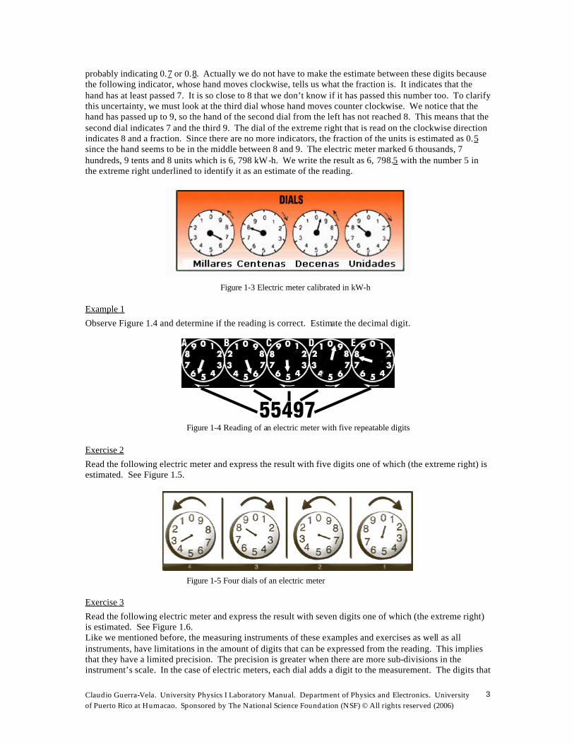
Read the following electric meter and express the result with five digits one of which (the extreme right) is estimated. See Figure 1.5.

Figure 1-5 Four dials of an electric meter

Exercise 3

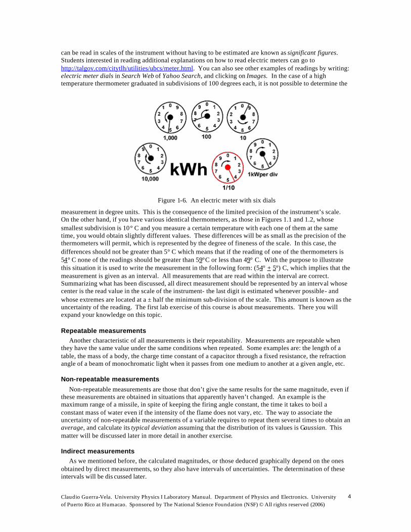
Read the following electric meter and express the result with seven digits one of which (the extreme right) is estimated. See Figure 1.6. Like we mentioned before, the measuring instruments of these examples and exercises as well as all instruments, have limitations in the amount of digits that can be expressed from the reading. This implies that they have a limited precision. The precision is greater when there are more sub-divisions in the instrument’s scale. In the case of electric meters, each dial adds a digit to the measurement. The digits that


4

can be read in scales of the instrument without having to be estimated are known as significant figures. Students interested in reading additional explanations on how to read electric meters can go to http://talgov.com/citytlh/utilities/ubcs/meter.html. You can also see other examples of readings by writing: electric meter dials in Search Web of Yahoo Search, and clicking on Images. In the case of a high temperature thermometer graduated in subdivisions of 100 degrees each, it is not possible to determine the

Figure 1-6. An electric meter with six dials

measurement in degree units. This is the consequence of the limited precision of the instrument’s scale. On the other hand, if you have various identical thermometers, as those in Figures 1.1 and 1.2, whose smallest subdivision is 10° C and you measure a certain temperature with each one of them at the same time, you would obtain slightly different values. These differences will be as small as the precision of the thermometers will permit, which is represented by the degree of fineness of the scale. In this case, the differences should not be greater than 5° C which means that if the reading of one of the thermometers is 54° C none of the readings should be greater than 59°C or less than 49° C. With the purpose to illustrate this situation it is used to write the measurement in the following form: (54° + 5°) C, which implies that the measurement is given as an interval. All measurements that are read within the interval are correct. Summarizing what has been discussed, all direct measurement should be represented by an interval whose center is the read value in the scale of the instrument- the last digit is estimated whenever possible- and whose extremes are located at a ± half the minimum sub-division of the scale. This amount is known as the uncertainty of the reading. The first lab exercise of this course is about measurements. There you will expand your knowledge on this topic.

Repeatable measurements Another characteristic of all measurements is their repeatability. Measurements are repeatable when they have the same value under the same conditions when repeated. Some examples are: the length of a table, the mass of a body, the charge time constant of a capacitor through a fixed resistance, the refraction angle of a beam of monochromatic light when it passes from one medium to another at a given angle, etc.

Non-repeatable measurements

Non-repeatable measurements are those that don’t give the same results for the same magnitude, even if these measurements are obtained in situations that apparently haven’t changed. An example is the maximum range of a missile, in spite of keeping the firing angle constant, the time it takes to boil a constant mass of water even if the intensity of the flame does not vary, etc. The way to associate the uncertainty of non-repeatable measurements of a variable requires to repeat them several times to obtain an average, and calculate its typical deviation assuming that the distribution of its values is Gaussian. This matter will be discussed later in more detail in another exercise.

Indirect measurements As we mentioned before, the calculated magnitudes, or those deduced graphically depend on the ones obtained by direct measurements, so they also have intervals of uncertainties. The determination of these intervals will be dis cussed later.


5

Example 2 The length of a table is measured using a meter stick graduated in centimeters. The value read is 81.3 cm. What is the uncertainty of the instrument and how should the result be expressed? Is this measurement repeatable? Solution

i. If the meter is graduated in centimeters, the uncertainty of the reading should be ± 0.5 cm, which is half the smallest sub-division, but this value has to be duplicated because there is an equal uncertainty by placing the zero of the meter on the left extreme of the table. So the uncertainty is ± 1cm.

ii. The result is expressed as (81.3 ± 1) cm. Notice that the digit 3 is underlined because it is estimated since the smallest subdivision of the ruler is one centimeter and it is not possible to read the tenths of a centimeter.

iii. Yes, the measurement is repeatable because every time that we repeat the measurement with the same ruler, in a similar way, we are going to obtain a result that will be within the uncertainty interval of the first measurement.

Example3

Mention a way of measuring directly the volume of a cube and a form of deducing its value from direct measurements. Solution

i. The direct measurement is made with a test tube where there is a known volume of water. We introduce the cube in the water and read the increase of the liquid level. The difference between the new and original level of water is the volume of the cube. This method makes it possible to measure directly the volume of irregular masses that cannot be deduced from direct measurements. See Figure1.7.

Figure 1-7 Direct measurement of the volume of an irregular object

ii. We measure the length of any of the sides of the cube, l, and calculate its volume from V = l3

Example 4. Mention a variable that can be measured directly as well as being deduced- excluding volume. Describe the procedure for both forms of measurements. Solution


6

i. The area of a rectangle can be measured directly by cutting it and placing it on a piece of graphic paper. We draw its outline and count the squares that are within the perimeter of the figure. Each square has an area of 1 mm squared

ii. Measuring the base and height of the rectangle and multiplying both make the indirect determination.

Example 5 What is the uncertainty associated with the reading of the temperature using a clinical domestic thermometer graduated in tenths of a degree? Solution

i. The uncertainty of the reading is half the smallest sub-division of the measuring instrument. In this case it is a half of a tenth of a degree, or ± 0.05° C. We do not duplicate this value as we did before in the case of the ruler because this time we only make one reading of the scale, which is the position of the upper extreme of the mercury column.

Example 6

Mention an example of a direct repeatable measurement and one non repeatable. Solution

i. The width of a sheet of paper is repeatable. ii. The temperature of the environment throughout the day is not repeatable.

Measurements with a metric ruler The common metric ruler is graduated in millimeters and permits readings of length with an uncertainty of no more than ± 0.5 mm. But we have to consider that when we measure, we have to place the zero at the initial point of the distance, so we really make two readings. This means that the uncertainty is twice ± 0.5 mm. or ± 1mm.

The vernier caliper The way the vernier caliper functions is a little bit complicated but elegant. This instrument permits to measure fractions of the smallest division of the scale given. Its use is common in a great number of precision instruments. Figure 1.8 presents a typical caliper.

Figure 1-8. The vernier caliper

The vernier scale, or movable ruler, is located on the ruler body, or main scale of the instrument. This part can move from one extreme to the other of the ruler. The line of the zero of the movable ruler coincides with the zero of the ruler when the caliper is completely closed. That is when there is no space between its outside pliers. We can see an excellent example of a virtual caliper which shows how it works at the following link http://members.shaw.ca/ron.blond/Vern.APPLET/. It is highly recommended for students to visit this site and practice using the caliper to understand how it works. When you open the page of this site observe that when the opening of the caliper is 1.0 mm the zero of the vernier scale aligns with the first division of a millimeter of the main scale. That means that the readings are indicated by the position of zero of the vernier scale of the instrument. When it is closed completely, we notice that nine divisions of


7

the main scale correspond to ten divisions of the vernier scale. The first line of the vernier, next to the zero line, shows a distance of 0.1 mm shorter of 1mm. If the caliper opens no more than 0.1 mm, the first line of the vernier would align with the first line of the main scale. If it opens 0.2 mm the second line of the vernier would align with the second line of the main scale and so on. In any measurements made with a caliper the tenths of a millimeter are indicated by the line of the vernier that is aligned with one of the lines of the ruler. Figure 1.9 shows a reading of 0.03 cm. The 0 appears as a result of being the first line of the

Figure 1-9 A reading of 0.3 mm

main scale that is found to the left of the zero line of the vernier, while the 3 corresponds to the only line of the vernier that coincides with that of the main scale. In the same way we can see that the reading of Figure 1.10 is 9.13 cm. The uncertainty of the reading of the caliper is + 0.05 mm, or ten times less than that of the metric ruler graduated in millimeters and it doesn’t have to be duplicated like in the ruler case because the zero of the caliper is established and fixed.

Figure 1-10 A reading of 9.13 cm

Exercise 4

Read the four measurements of Figure 1.11.

Figure 1-11 Four readings with a vernier caliper

The micrometer Another instrument used for measuring length is the micrometer. See Figure 1.12. The micrometer works with a screw that produces the advancement of half a millimeter (0.5mm) of the spindle in each turn .The thimble has a scale graduated into 50 divisions, each one equaling 0.01mm. The uncertainty of the reading of the micrometer is + 0.005 mm. It is ten times smaller than that of the caliper. The barrel where the thimble turns is graduated in divis ions of 0.5 mm. We notice that the barrel’s scale has divisions in the upper and lower parts of the horizontal line of reference. The divisions of the upper part show the


8

millimeters while those of the lower part show halves of millimeters. To make a measurement, you first read the horizontal scale indicated by the left edge of the thimble, and then you add the number that is found aligned to the horizontal line of the barrel, which we have called the reference line. In the extreme right of the micrometer shown in figure 1.12 there is a ratchet that limits the magnitude of the pressure that can be applied to the measured object.

Figure 1-12 Micrometer

When using this instrument, you must have the precaution of closing it by its ratchet. This avoids closing it tight enough as to cause a permanent damage to the screw. Another important precaution is checking if the zero of the thimble is aligned to the reference line when the spindle is closed completely against the anvil. If the reading is not zero, you must add or subtract the correction factor to the measurement. Failure to do this will bring a systematic error to your measurement. If the micrometer has a reading greater than zero, when closed, then this amount must be subtracted from the measurement obtained. If the micrometer reads zero before being completely closed, the number of divisions that must be turned to close it completely must be added to the final measurement. It is also possible to correct these systematic errors by calibrating the instrument. If the one on your laboratory bench is at fault, report it to your lab instructor so the lab technician can fix it. As an example you should note that the reading of Figure 1.13 is 8.115 mm.

Figure 1-13 How to read a micrometer


9

In the following site you can find more information on how to read the micrometer as well as a short exam of this topic http://www.colchsfc.ac.uk/physics/APhysics2000/Module1/Materials/hotpot/micrometer.htm.

Uncertainties As we mentioned before, the measurements of physical variables are associated with an uncertainty that comes from the reading of the scale of the measuring instrument. This uncertainty can be obtained through different ways, depending of the type of measurement. In this first practice we will refer only to repeatable measurements. Repeatable measurements are those that give the same result each time they are made with a particular instrument. The uncertainty associated with repeatable measurements comes from the reading of the scale of the instrument. If the instrument has a way to fix its zero reading, as the caliper, or to adjust it as in the micrometer, and some electronic instruments, the uncertainty of the reading will be half of the smallest division of the scale. If this is not the case, then the uncertainty is the complete sub division. Since a ruler is not an instrument where the zero can be adjusted, then the uncertainty equals the value of its smallest sub-division. If it is graduated in millimeters, it will be + 1mm. In the case of the caliper, the uncertainty of the reading is ± 0.05 mm because tenths of millimeters can be read. With the micrometer it is + 0.005 mm.

Example 7. Typical measurement with a ruler graduated in millimeters. You measure the width of a sheet of paper and obtain 21.7 cm. The result should be expressed correctly like (21.7 + 0.1) cm. The uncertainty of 1mm is associated with the reading (remember that 1mm = 0.1 cm). If this measurement is repeated with any ruler graduated in millimeters and the number obtained is no less than 21.7-0.1= 21.6 cm or nor greater than 21.7 + 0.1= 21.8 cm, then it is said that the measurement is repeatable. In a more formal way: a measurement is repeatable when it yields results whose differences are within the uncertainty of the reading of the instrument

Example 8. Typical measurement with a caliper

The width of a plastic ruler was measured and a value of 2.87 cm was obtained. The result should be expressed correctly as (2.87 + 0.005) cm that shows that the width of ruler is 2.87 cm more or less the uncertainty of 0.005 cm related to the reading.

Example 9. Typical measurement with a micrometer Since the micrometer is a more sophisticated instrument than a ruler and a caliper, its use requires some special care. First, always turn it by its ratchet to limit the pressure on the measured object. This must be made slowly to prevent closing the spindle by inertia. It is unfortunate to find a micrometer with the zero of its thimble not aligned with the reference line of the barrel when fully closed. Let us suppose that the spindle closes by touching the anvil without reading zero and the difference estimated is 6 tenths of a sub division. Since this is an estimated number, it is the result of a subjective perception in the reading. If we measure the thickness of a plate and the result is 1.205 mm, we must remember that we are measuring 0.006 mm in excess so it must be subtracted from the result. That is 1.205 – 0.006 = 1.199 mm. The uncertainty in the reading of the micrometer is of + 0.005 mm so the final result is (1.199 ± 0.005) mm.

How to write the result of a measurement

In this course all repeatable measurements should be expressed as xxx δ±= , where x represents the

result and xδ , the absolute uncertainty related to the reading of the scale. Notice that the measurement with its uncertainty is represented with just one letter without the bar on the top. Please, if you have any questions related to ideas explained up to the moment, consult your lab instructor.


10

Relative percentile uncertainty or delta percentile Relative percentile uncertainty of any physical variable x is defined as,

100% ×δ=∆xx Equation 1-1

where ∆ is the Greek Capital delta. This amount is used to express the degree of precision of a measurement. From examples 7 and 8 above we obtain the following relative percentile uncertainties:

Instrument ∆% Ruler

%46.01007.211.0 =×

Caliper %17.0100

87.2005.0 =×

The smaller the ∆%, the better the precision. Most of the measurements in this lab will have a ∆% ≈ 2%. Another use of ∆% is to facilitate the calculations of the uncertainties’ propagation that are made with direct measurements as shown in the following section.

Uncertainty propagation Indirect measurements have also uncertainties that come from the propagation of uncertainties in the direct measurements, which allow us to calculate the values of the deduced measurements. If we want to calculate the surface area or volume of a regular solid, such as a cube or sphere, from their linear dimensions, we have to find out the uncertainties associated with the calculated results. Let us suppose that a physical variable z is the product of three independent variables u, v, and w, that is z = uvw. Since u, v, and w are the result of direct measurements, they have uncertainties in their values, this means that,

uuu δ±= , vvv δ±= , y www δ±= . The corresponding value of ∆% in z comes from the following equation,

222

100100100100%

×

δ+

×

δ+

×

δ=×

δ≡∆

w

w

v

v

u

u

z

z Equation 1-2

and,

100%∆×=δ zz Equation 1-3

with wvuz = .

Example 10 Let us suppose that we measure the three sides of a block with a ruler graduated in millimeters. The following results are obtained: Length: l = (6.35 ± 0.1) cm

Width: a = (4.65 ± 0.1) cm, and Thickness: g = (2.20 ± 0.1) cm


11

We want to calculate the volume of the block from these direct measurements and write the result in the

form, of VVV δ±= . What would it be the relative percentile uncertainty 100×δVV

and the absolute

uncertainty Vδ of the volume? Solution: The procedure requires:

i. The determination of ∆% of each measurement

%75.110053.61.0

100 =×=×δ

ll

%51.210056.41.0

100 =×=×δ

a

a

%55.410002.21.0100 =×=×δ

g

g

ii. The square root of the sum of the squares of these three quantities because V = lag and in these

cases we have to apply Equation 1.2

222

100100100100

×

δ+

×

δ+

×

δ=×

δ

g

g

a

a

V

V

ll =

= ( ) ( ) ( )222 55.451.275.1 ++ = 5.27%

iii. The calculation of the volume

gaV l= = 6.35 × 4.65 × 2.20 = 65.0 cm3

iv. The calculation of the absolute uncertainty of the volume using Equation 1.3

3cm4.3100

72.50.65100

% =×

=∆×=δ VV

v. The final result for the volume should be expressed as

V = (65.0 ± 3.4) cm3

Notice that the result only has three digits for the value V and two for the value Vδ . This is because the results come from calculations made with numbers that only have two repeatable digits and one estimated. Then the final results should also have as much as two repeatable and one estimated number. The number 3.43 was rounded to 3.4 because the value of the volume is uncertain in the first decimal.

Exercise 5 We measure the sides of a sheet of paper with a ruler graduated in millimeters and obtain the following

results; length, l = 27.87 cm and width a = 21.58 cm.


12

1. Write the uncertainties of the readings of l and a 2. Calculate:

a. The area of the sheet of paper, aA ×= l ,

b. The relative percentile uncertainties of l and a using: 100 and 100δ δ× ×ll

aa

c. The relative percentile uncertainty of the area

22

100100100

×

δ+

×

δ=×

δ

a

a

A

A

ll

d. The absolute uncertainty of the area, Aδ e. Write the result in the form of AAA δ±=

Answers: 0.1 cm, 0.1 cm, 601.43 cm2, 0.36%, 0.46%, 0.59%, 3.52 cm2, (601.43 ± 3.52) cm2

Example 11 We measure the diameter of a ball bearing with a micrometer. The micrometer is completely closed but still reads 0.087 mm, which means that it is not adjusted to zero but reads an amount in excess. When the ball bearing is measured we read its diameter as 25.435 mm. We subtract the amount in excess and obtain 25.348 mm. The uncertainty of the reading of the micrometer is 0.005mm. Calculate the volume of the sphere and its absolute uncertainty. Express the result of the measurement with its absolute uncertainty. Solution

i. Remember that the formula for the volume of a sphere is,

3

6dV π= ,

Where d represents the diameter and V the volume. So

33 mm 7.527,8mm) 834.25(6

=×π

=V

ii. In this particular case, the absolute uncertainty is given by the following equation that the lab

instructor will deduce in class

Vd

dV

δ=δ 3 ,

Thus,

604.57.527,8834.25

005.03 =×

=δV mm3

Finally,

iii. V = (8.528 ± 0.005) cm3 iv. Notice that we have converted the result into cm3. Remember that 1 cm = 10 mm and 1 cm3 =

1000 mm3


13

Not all physical variables can be measured directly since there are no measuring instruments for all of them. In these cases, it is easier and advisable to obtain their value by means of calculations with direct measurements. An example of this is the density of solids, ρ = m /V, which is the ratio of mass per volume of a body . These two variables can be measured directly, and from their values, a density can be calculated.

Example 12 Determine the density of the ball bearing of example 11 knowing that it has a mass of 23.2 g, measured with a balance graduated in grams. Express the result with its absolute uncertainty Solution:

i. The available data are: V = (8.528 ± 0.005) cm 3 and m = (23.2 ± 0.5) g. The uncertainty in the reading of the balance is ± 0.5 g because its minimum division is 1 g and its zero is adjustable

ii. The relative percentile uncertainties are:

%057.0100528.8005.0100 =×=×δ

VV

And

%2.21002.235.0

100 =×=×δmm

iii. Also, the relative percentile uncertainty of density, in agreement with equation 1.2, which also applies for quotients of variables, is:

( ) ( ) %...mmd

VVd

??d

22220570100100100 2222

=+=

×+

×=×

iv. Now, in agreement with equation 1.3, we obtain,

3cm

g1.0 06.072.2220.0

528.82.23

022.0100

2.2==×=

×=ρ×=ρδ

v. Finally,

3cm

g 1.07.2 ±=ρ

The density, like the heat capacity, Young’s modulus, refractive index, coefficient of thermal expansion, dielectric constant, and many other physical variables, are characteristic properties of materials. This means that each material is characterized by its value of these variables. A certain density, whose value we can find in the literature, for example, characterizes aluminum. Consulting physics books, or looking in the Internet, we will find that the density of aluminum is 2.7 gm/cm3. (See, for example, the following connection where there is information on a variety of subjects in multiple disciplines: http://en.wikipedia.org/wiki/). When comparing the density that we measured, with the reported one in the literature for aluminum, we notice that they are the same; therefore, the sphere is made of this material. It not always happens that the results of the measurements of characteristic properties are equal to the values


14

reported in the literature. In fact, the most common situation is to find differences between both. One has to evaluate these differences with the following formula:

measured reported

reportedDifference % 100

x x

x

−= ×

Where xmeasured is the value of the variable obtained in the laboratory, and xreported is the value found in the literature. Next we included a table with the values of densities for some gases and common solids according to reports in the literature:

Table of selected densities Material Density (g/cm3)

Olive oil 0.92 Steel 7.9 Dry air (20 °C, 1 atm) 1.21 × 10 -3 Aluminum 2.7 Concrete 2 Copper 8.9 Cork 0.25 Diamond 3.3 Helium (0 °C, 1 atm) 0.178 × 10 -3 Hydrogen (0 °C, 1 atm) 0.090 × 10 -3 Ice 0.917 Iron 7.9 Wood of raft 0.12 Mercury 13.6 Nickel 8.8 Gold 19.3 Oxygen (0 °C, 1 atm) 1.43 × 10 -3 Silver 10.5 Platinum 21.5 Glass 2.5

The material presented in this introductory chapter is the minimum necessary to begin your lab course. If you still have difficulty in understanding this material when you finish reading this chapter, you should ask your laboratory instructor to clarify your doubts. You must keep in mind that the work in a lab is not trivial. You must do the tasks carefully, knowing what you are looking for and how to find it.

Materials

An aluminum block A steel ball

Measuring Instruments

A plastic ruler of 30 cm (graduated in millimeters) A caliper (graduated in millimeters), and A micrometer

Procedure

1. Measure the length l, the width a and the thickness g of the aluminum using:

a. A ruler b. The caliper, and c. The mic rometer


15

2. Write the results, with their absolute uncertainties in Table 1 of the lab report 3. Calculate the relative percentile uncertainties of each measurement and write them in Table 2 of

the lab report.

4. Calculate the volume, V , of the block using the equation gaV ××= l and the values of

, anda gl measured with the ruler. Write the results in the lab report.

5. Repeat point 4 with the values obtained in the caliper. Write the results in your lab report. 6. Repeat point 4 with the values obtained with the micrometer. Write the results in your lab report.

7. Calculate ∆% of the volume using the data from Table 2 for the ruler measurements and write the

results in the lab report.

8. Calculate ∆% of the volume using the data of Table 2 for the caliper measurements and write the results in the lab report.

9. Calculate the ∆% of the area using the data of Table 2 of the micrometer measurements and write

the result in the lab report.

10. Use the equation ( )%100VVδ = ∆ × to find the absolute uncertainty of the volume obtained from

the measurements made with the ruler.

11. Repeat step 10 with the measurements made with the caliper.

12. Repeat step 10 with the measurements made with the micrometer. Make sure to substitute the area for the volume.

13. Write the volumes and areas with their absolute uncertainties in Table 3 of the lab report.

14. Measure the diameter, d, of the metal sphere with the vernier and the micrometer, and write each

one, with its uncertainty in the reading, in the first column of Table 4 of the laboratory report

15. Calculate the percentage relative uncertainty for each instrument, and write each one, in the second column of Table 4 of the laboratory report

16. Calculate the volume of the sphere, for each measurement, and write each one, in the third column of Table 4 of the laboratory report

17. Calculate the absolute uncertainties of the volumes, for each measurement, and write each one, in the fourth column of Table 4 of the laboratory report

18. Express the volumes with its absolute uncertainties in the fifth column of Table 4 of the laboratory report

19. Measure the mass of the sphere with a balance graduated in tenths of grams and write it with its uncertainty in the reading

20. Calculate the percentage relative uncertainty of the mass and write it in the lab report

21. Calculate the density of the sphere using the volume measured with the micrometer, whose value appears in Table 4 of the report, and the measured mass

22. Calculate the percentage relative uncertainty of the density of the sphere and write it down in the laboratory report


16

23. Calculate the absolute uncertainty of the density of the sphere and write it down in the laboratory report

24. Write down the density of the sphere with its absolute uncertainty in the laboratory report

25. Measure the mass of the metallic block and calculate its density, with its absolute uncertainty, using the volume measured with the micrometer and repeating the steps of the procedure from 20 to 24

26. Answer the questions in the report and hand it in to your instructor before leaving the laboratory


17

Experiment 1 Laboratory Report

Measurements of length, area, volume, and density

Section _______ Laboratory bench number _______ Date: ______________________________________ Students: ________________________________________________________ ________________________________________________________ ________________________________________________________ ________________________________________________________ 1. Step 1 of the procedure, and so on … 2.

Table 1 Instrument cm )( ll δ± cm )( aa δ± cm )( gg δ±

Ruler

Vernier

Micrometer

This micrometer only measures up to 2.54 cm

3.

Table 2 Instrument

100×δll

100×δaa

100×δgg

Rule

Vernier

Micrometer

There are no data

4. Calculation of the volume from the measurements made with the ruler:

) ( ) ( ) ( =××== gaV l ________________ cm3 5. Calculation of the volume from the measurements made with the vernier:

) ( ) ( ) ( =××== gaV l ________________ cm3 6. Calculation of the area from the measurements made with the micrometer:


18

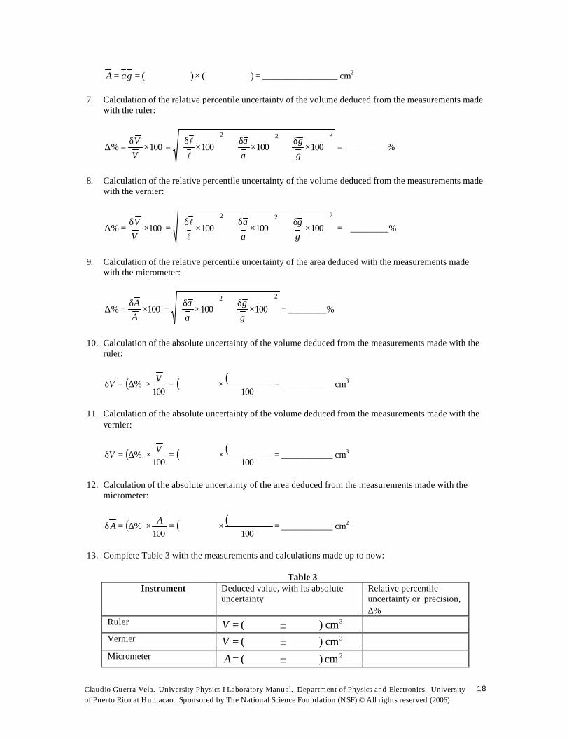
=×== ) ( ) ( gaA ________________ cm2 7. Calculation of the relative percentile uncertainty of the volume deduced from the measurements made

with the ruler:

222

100100100100%

×

δ+

×

δ+

×

δ=×

δ=∆

g

g

a

a

V

V

ll

= _________%

8. Calculation of the relative percentile uncertainty of the volume deduced from the measurements made

with the vernier:

=

×

δ+

×

δ+

×

δ=×

δ=∆

222

100100100100%g

g

a

a

V

V

ll

________%

9. Calculation of the relative percentile uncertainty of the area deduced with the measurements made

with the micrometer:

22

100100100%

×

δ+

×

δ=×

δ=∆

g

g

a

aAA

= ________%

10. Calculation of the absolute uncertainty of the volume deduced from the measurements made with the

ruler:

( ) ( ) ( ) =×=×∆=δ100

100

% VV ___________ cm3

11. Calculation of the absolute uncertainty of the volume deduced from the measurements made with the

vernier:

( ) ( ) ( ) =×=×∆=δ100

100

% VV ___________ cm3

12. Calculation of the absolute uncertainty of the area deduced from the measurements made with the

micrometer:

( ) ( ) ( ) =×=×∆=δ100

100

% AA ___________ cm2

13. Complete Table 3 with the measurements and calculations made up to now:

Table 3 Instrument Deduced value, with its absolute

uncertainty Relative percentile uncertainty or precision, ∆%

Ruler 3cm ) ( ±=V

Vernier 3cm ) ( ±=V

Micrometer 2cm ) ( ±=A


19

14. And 15. And 16. And 17. And 18.

Table 4 Instrument dd δ± (cm)

ddδ

3

6dV

π= (cm) 3 Vδ (cm3) V (cm3)

Vernier ±

±

Micrometer

±

±

19. Mass of the sphere

m = _______ ±_______ g 20. Relative percentile uncertainty of the mass

100% ×δ

=∆mm

= _______%

21. Density of the sphere

Vm=ρ = _______ g/cm3

22. Relative percentile uncertainty of the density

22

100100100%

×δ+

×δ=×

ρρδ=∆

VV

mm

= _________%

23. Absolute uncertainty of the density of the sphere

100%)(

ρ×∆=ρδ = ________ g/cm3

24. Value of the density with its absolute uncertainty

ρ= (__________ ± __________) g/cm 3


20

25. Show, in the space provided below, the result of the measurement of the aluminum block mass with its uncertainty in the reading, and all the steps and calculations that lead to the final result of the density of the block with its absolute uncertainty


21

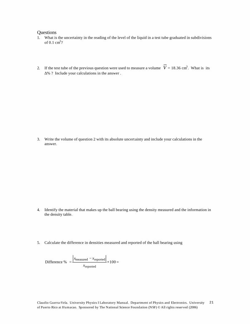
Questions 1. What is the uncertainty in the reading of the level of the liquid in a test tube graduated in subdivisions

of 0.1 cm3?

2. If the test tube of the previous question were used to measure a volume V = 18.36 cm3. What is its ∆% ? Include your calculations in the answer .

3. Write the volume of question 2 with its absolute uncertainty and include your calculations in the

answer. 4. Identify the material that makes up the ball bearing using the density measured and the information in

the density table. 5. Calculate the difference in densities measured and reported of the ball bearing using

measured reported


x x

x

−= × =


22

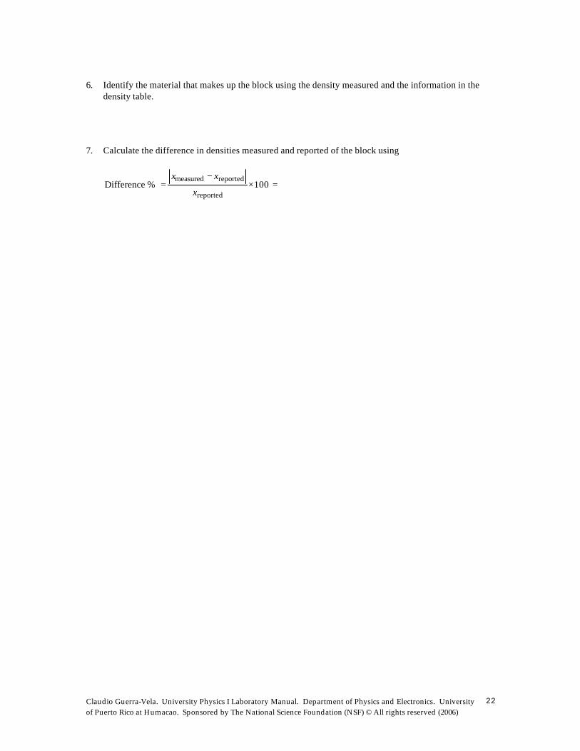
6. Identify the material that makes up the block using the density measured and the information in the

density table. 7. Calculate the difference in densities measured and reported of the block using

measured reported


x x

x

−= × =


23

Experiment 1 Questions

Measurements of length, area, volume and density

This questionnaire has some typical questions on experiment 1. All students who are taking the laboratory course of University Physics I must be able to correctly answer it before trying to make the experiment. 1. We speak of deduced values when they

a. are estimated b. are obtained in the conclusions of a lab report c. come from research d. are obtained by reading directly from the scale of the measuring instrument e. are obtained through calculations or graphics that at the same time come from values

measured directly 2. The uncertainty in the reading of a vernier caliper is:

a. ± 1.0 cm b. ± 0.05 mm c. ± ½” d. ± 0.01 cm e. ± 0.5 mm

3. A measurement is direct when it

a. comes directly from literature b. is obtained from calculations or graphics c. is obtained by asking its value from the person who made it d. has no other way of being obtained e. is obtained by reading directly from the scale of the measuring instrument

4. The graphical determination of a value

a. is a value obtained directly b. is never reliable c. is a deduced value d. is not the result of a measurement e. should be avoided at all cost

5. The acceleration, a, of an object obtained from the equation a = 2d/t2 where the distance d and time t,

have known values measured directly, a. represents a case of indirect measurement b. requires the use of graphical analysis c. has an uncertainty of ± 0.1 cm d. is not possible to obtain the value of the acceleration with this equation e. represents a case of direct measurement

6. Indirect measurements are:

a. the length and the time measured with a ruler and chronometer b. those obtained by asking other persons c. those that have not been determined by any instrument that measure them directly d. those that cannot be measured like love, thirst, being tired, etc. e. those obtained by reading the scale of a measuring instrument


24

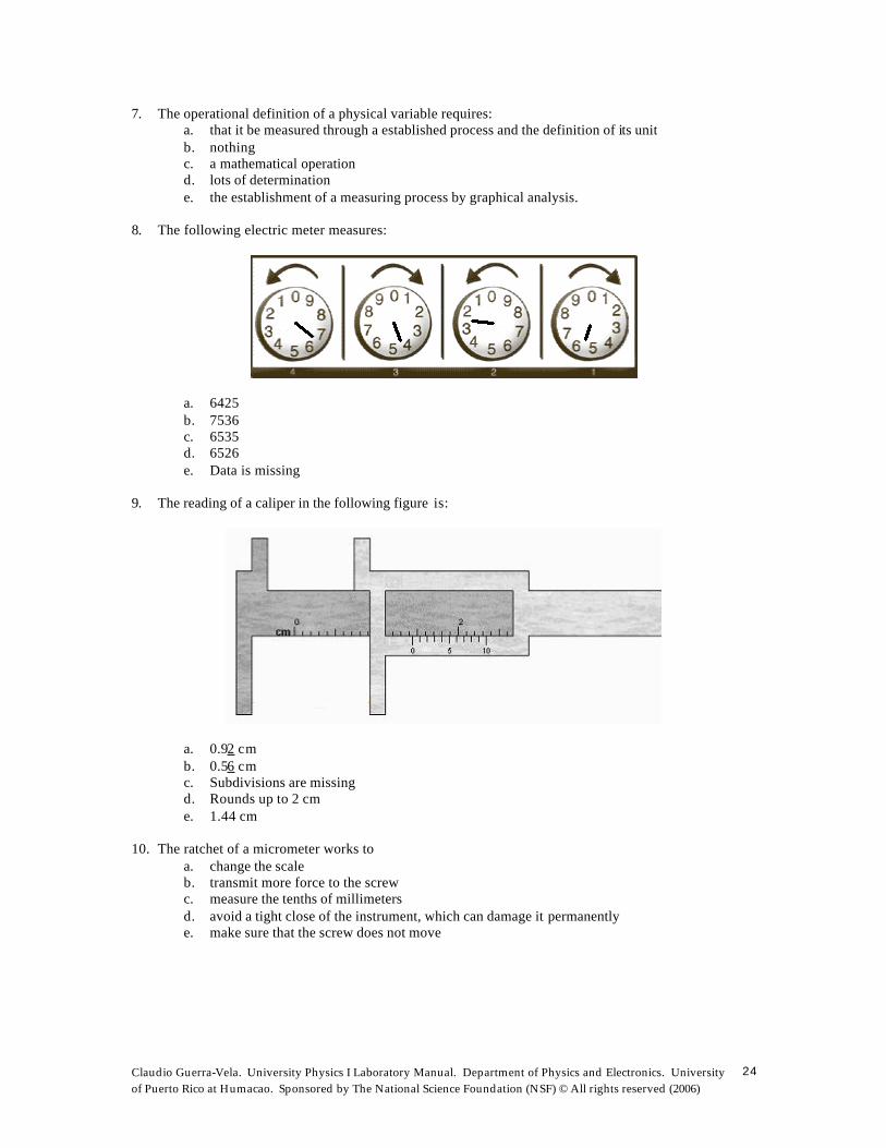
7. The operational definition of a physical variable requires: a. that it be measured through a established process and the definition of its unit b. nothing c. a mathematical operation d. lots of determination e. the establishment of a measuring process by graphical analysis.

8. The following electric meter measures:

a. 6425 b. 7536 c. 6535 d. 6526 e. Data is missing

9. The reading of a caliper in the following figure is:

a. 0.92 cm b. 0.56 cm c. Subdivisions are missing d. Rounds up to 2 cm e. 1.44 cm

10. The ratchet of a micrometer works to

a. change the scale b. transmit more force to the screw c. measure the tenths of millimeters d. avoid a tight close of the instrument, which can damage it permanently e. make sure that the screw does not move


25

11. The width of a sheet of paper is w = (3.17 ± 0.1) cm. The relative percentile uncertainty is: a. ± 0.1% b. ± 1% c. ± 3.15 % d. ± 2.3 % e. ± 0.3%

12. The measurements of width and length of a table have relative percentile uncertainties of ± 1.2 % and

± 0.56 % respectively. The relative percentile uncertainty of the area is: a. ± 1.76 % b. Data is missing c. ± 1.2 % d. ± 0.6 % e. ± 1.32%

13. The uncertainty of a ruler graduated in millimeters is:

a. ± 0.005 mm b. ± 0.05 mm c. ± 0.5 cm d. It depends what is being measured. e. ± 1 mm

14. The uncertainty in the reading of a micrometer is:

a. ± 0.005 mm b. ± 0.05 mm c. ± 0.5 cm d. it depends on what will be measured e. ± 1 mm

Documents

Measurements of Lenght, Area, Volume and Density