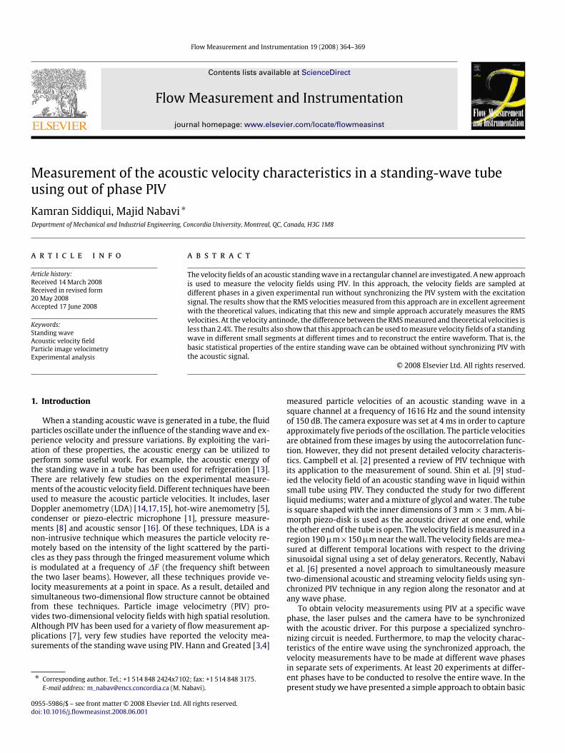
Flow Measurement and Instrumentation 19 (2008) 364–369

Contents lists available at ScienceDirect

Flow Measurement and Instrumentation

journal homepage: www.elsevier.com/locate/flowmeasinst

Measurement of the acoustic velocity characteristics in a standing-wave tubeusing out of phase PIVKamran Siddiqui, Majid Nabavi ∗Department of Mechanical and Industrial Engineering, Concordia University, Montreal, QC, Canada, H3G 1M8

a r t i c l e i n f o

Article history:Received 14 March 2008Received in revised form20 May 2008Accepted 17 June 2008

Keywords:Standing waveAcoustic velocity fieldParticle image velocimetryExperimental analysis

a b s t r a c t

The velocity fields of an acoustic standingwave in a rectangular channel are investigated. A new approachis used to measure the velocity fields using PIV. In this approach, the velocity fields are sampled atdifferent phases in a given experimental run without synchronizing the PIV system with the excitationsignal. The results show that the RMS velocities measured from this approach are in excellent agreementwith the theoretical values, indicating that this new and simple approach accurately measures the RMSvelocities. At the velocity antinode, the difference between the RMSmeasured and theoretical velocities isless than 2.4%. The results also show that this approach can be used tomeasure velocity fields of a standingwave in different small segments at different times and to reconstruct the entire waveform. That is, thebasic statistical properties of the entire standing wave can be obtained without synchronizing PIV withthe acoustic signal.

© 2008 Elsevier Ltd. All rights reserved.

1. Introduction

When a standing acoustic wave is generated in a tube, the fluidparticles oscillate under the influence of the standingwave and ex-perience velocity and pressure variations. By exploiting the vari-ation of these properties, the acoustic energy can be utilized toperform some useful work. For example, the acoustic energy ofthe standing wave in a tube has been used for refrigeration [13].There are relatively few studies on the experimental measure-ments of the acoustic velocity field. Different techniques have beenused to measure the acoustic particle velocities. It includes, laserDoppler anemometry (LDA) [14,17,15], hot-wire anemometry [5],condenser or piezo-electric microphone [1], pressure measure-ments [8] and acoustic sensor [16]. Of these techniques, LDA is anon-intrusive technique which measures the particle velocity re-motely based on the intensity of the light scattered by the parti-cles as they pass through the fringed measurement volume whichis modulated at a frequency of ∆F (the frequency shift betweenthe two laser beams). However, all these techniques provide ve-locity measurements at a point in space. As a result, detailed andsimultaneous two-dimensional flow structure cannot be obtainedfrom these techniques. Particle image velocimetry (PIV) pro-vides two-dimensional velocity fields with high spatial resolution.Although PIV has been used for a variety of flowmeasurement ap-plications [7], very few studies have reported the velocity mea-surements of the standing wave using PIV. Hann and Greated [3,4]

∗ Corresponding author. Tel.: +1 514 848 2424x7102; fax: +1 514 848 3175.E-mail address:m_nabav@encs.concordia.ca (M. Nabavi).

0955-5986/$ – see front matter© 2008 Elsevier Ltd. All rights reserved.doi:10.1016/j.flowmeasinst.2008.06.001

measured particle velocities of an acoustic standing wave in asquare channel at a frequency of 1616 Hz and the sound intensityof 150 dB. The camera exposure was set at 4 ms in order to captureapproximately five periods of the oscillation. The particle velocitiesare obtained from these images by using the autocorrelation func-tion. However, they did not present detailed velocity characteris-tics. Campbell et al. [2] presented a review of PIV technique withits application to the measurement of sound. Shin et al. [9] stud-ied the velocity field of an acoustic standing wave in liquid withinsmall tube using PIV. They conducted the study for two differentliquidmediums; water and amixture of glycol andwater. The tubeis square shapedwith the inner dimensions of 3mm× 3mm. A bi-morph piezo-disk is used as the acoustic driver at one end, whilethe other end of the tube is open. The velocity field ismeasured in aregion 190µm×150µmnear thewall. The velocity fields aremea-sured at different temporal locations with respect to the drivingsinusoidal signal using a set of delay generators. Recently, Nabaviet al. [6] presented a novel approach to simultaneously measuretwo-dimensional acoustic and streaming velocity fields using syn-chronized PIV technique in any region along the resonator and atany wave phase.To obtain velocity measurements using PIV at a specific wave

phase, the laser pulses and the camera have to be synchronizedwith the acoustic driver. For this purpose a specialized synchro-nizing circuit is needed. Furthermore, to map the velocity charac-teristics of the entire wave using the synchronized approach, thevelocity measurements have to be made at different wave phasesin separate sets of experiments. At least 20 experiments at differ-ent phases have to be conducted to resolve the entire wave. In thepresent studywe have presented a simple approach to obtain basic

K. Siddiqui, M. Nabavi / Flow Measurement and Instrumentation 19 (2008) 364–369 365

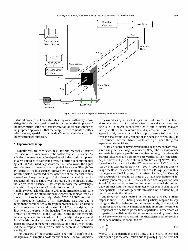
Fig. 1. Schematic of the experimental setup and instrumentation.

statistical properties of the entire standing wave without synchro-nizing PIV with the acoustic signal. In addition to the simplicity ofthe experimental setup and instrumentation, another advantage ofthe proposed approach is that the sample size to compute the RMSvelocity at any spatial location is significantly larger than that forthe synchronized approach.

2. Experimental setup

Experiments are conducted in a Plexiglas channel of squarecross-section. The inner cross-section of the channel is 7×7 cm.An8 � electro-dynamic type loudspeaker with the maximum powerof 50 W is used as the acoustic driver. A function generator modelAgilent 33120A is used to generate the sinusoidal wave. The signalfrom the function generator is amplified by an amplifier (MPA-25, Realistic). The loudspeaker is driven by this amplified signal. Amovable piston is attached to the other end of the channel, whichallowed to change the length of the channel depending on thefrequency of the acoustic driver (see Fig. 1). In the present study,the length of the channel is set equal to twice the wavelengthat a given frequency to allow the formation of two completestandingwaves inside the channel. Air at the atmospheric pressureis used as theworking fluid. The acoustic pressure ismeasured by acondenser microphone cartridge Model 377A10 PCB Piezotronics.The microphone consists of a microphone cartridge and amicrophone preamplifier. A preamplifier Model 426B03 is used inorder to measure the sound pressure level. The cartridge screwsdirectly onto the preamplifier housing. The frequency response isalmost flat between 5 Hz and 100 kHz. During the experiments,the microphone is placed inside a hole in the adjustable piston andflashed with the piston inner surface. Thus, the microphone andpiston are always at the same position i.e. at the pressure antinode,and the microphone measures the maximum pressure fluctuation(see Fig. 1).The thickness of the channel walls is 6 mm. To confirm that

the rigid wall assumption holds for this channel, the wall vibration

is measured using a Brüel & Kjær laser vibrometer. The laservibrometer consists of a Helium–Neon laser velocity transducertype 8323, a power supply type 2815 and a signal analyzerunit type 2035. The maximum wall displacement is found to beapproximately one micron which is approximately 200 times lessthan the maximum displacement of the acoustic driver. Thus, itis concluded that the channel walls are rigid under the givenexperimental conditions.The two-dimensional velocity fields inside the channel aremea-

sured using particle image velocimetry (PIV). The measurementsare made in a plane parallel to the channel length at the mid-channel location (i.e. 3.5 cm from both vertical walls of the chan-nel) as shown in Fig. 1. A Continuum Minilite 25 mJ Nd:YAG laseris used as a light source for the PIV measurements. A CCD camera(JAI CV-M2) with the resolution of 1600 × 1200 pixels is used toimage the flow. The camera is connected to a PC equipped with aframe grabber (DVR Express, IO Industries, London, ON, Canada)that acquired 8-bit images at a rate of 30 Hz. A four-channel digi-tal delay generator (555-4C, Berkeley Nucleonics Corporation, SanRafael CA) is used to control the timing of the laser light pulses.Olive oil mist with the mean diameter of 0.5 µm is used as thetracer particles. An aerosol generator (Lavision Inc., Ypsilanti MI) isused to generate the oil mist.An important issue related to the tracer particles is their

response time. That is, how quickly the particles respond to anychange in the flow behavior. In the present study, the density ofthe tracer particles is much higher than that of the air; therefore, itis important to find the response time of particles. Furthermore, asthe particles oscillate under the action of the standing wave, thisissue becomes evenmore critical. The characteristic response timeof the seed particles is computed by,

TP =uTg

(1)

where, TP is the particle response time, uT is the particle terminalvelocity and g is the acceleration due to gravity [12]. The terminal

366 K. Siddiqui, M. Nabavi / Flow Measurement and Instrumentation 19 (2008) 364–369

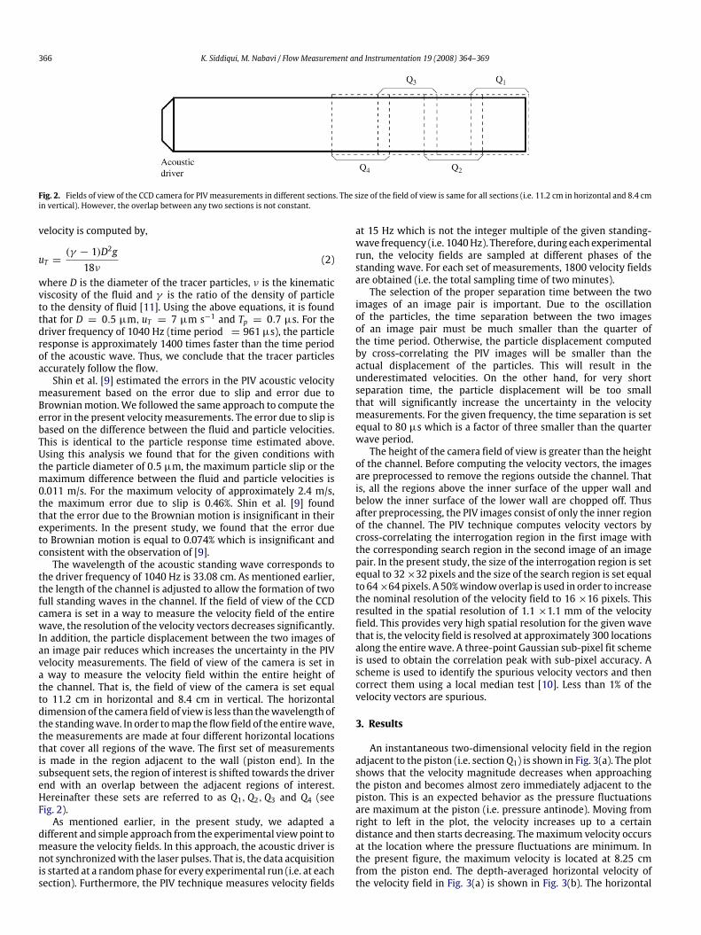
Fig. 2. Fields of view of the CCD camera for PIV measurements in different sections. The size of the field of view is same for all sections (i.e. 11.2 cm in horizontal and 8.4 cmin vertical). However, the overlap between any two sections is not constant.

velocity is computed by,

uT =(γ − 1)D2g18ν

(2)

where D is the diameter of the tracer particles, ν is the kinematicviscosity of the fluid and γ is the ratio of the density of particleto the density of fluid [11]. Using the above equations, it is foundthat for D = 0.5 µm, uT = 7 µm s−1 and Tp = 0.7 µs. For thedriver frequency of 1040 Hz (time period = 961 µs), the particleresponse is approximately 1400 times faster than the time periodof the acoustic wave. Thus, we conclude that the tracer particlesaccurately follow the flow.Shin et al. [9] estimated the errors in the PIV acoustic velocity

measurement based on the error due to slip and error due toBrownianmotion.We followed the same approach to compute theerror in the present velocity measurements. The error due to slip isbased on the difference between the fluid and particle velocities.This is identical to the particle response time estimated above.Using this analysis we found that for the given conditions withthe particle diameter of 0.5 µm, the maximum particle slip or themaximum difference between the fluid and particle velocities is0.011 m/s. For the maximum velocity of approximately 2.4 m/s,the maximum error due to slip is 0.46%. Shin et al. [9] foundthat the error due to the Brownian motion is insignificant in theirexperiments. In the present study, we found that the error dueto Brownian motion is equal to 0.074% which is insignificant andconsistent with the observation of [9].The wavelength of the acoustic standing wave corresponds to

the driver frequency of 1040 Hz is 33.08 cm. As mentioned earlier,the length of the channel is adjusted to allow the formation of twofull standing waves in the channel. If the field of view of the CCDcamera is set in a way to measure the velocity field of the entirewave, the resolution of the velocity vectors decreases significantly.In addition, the particle displacement between the two images ofan image pair reduces which increases the uncertainty in the PIVvelocity measurements. The field of view of the camera is set ina way to measure the velocity field within the entire height ofthe channel. That is, the field of view of the camera is set equalto 11.2 cm in horizontal and 8.4 cm in vertical. The horizontaldimension of the camera field of view is less than thewavelength ofthe standingwave. In order tomap the flow field of the entirewave,the measurements are made at four different horizontal locationsthat cover all regions of the wave. The first set of measurementsis made in the region adjacent to the wall (piston end). In thesubsequent sets, the region of interest is shifted towards the driverend with an overlap between the adjacent regions of interest.Hereinafter these sets are referred to as Q1,Q2,Q3 and Q4 (seeFig. 2).As mentioned earlier, in the present study, we adapted a

different and simple approach from the experimental viewpoint tomeasure the velocity fields. In this approach, the acoustic driver isnot synchronizedwith the laser pulses. That is, the data acquisitionis started at a randomphase for every experimental run (i.e. at eachsection). Furthermore, the PIV technique measures velocity fields

at 15 Hz which is not the integer multiple of the given standing-wave frequency (i.e. 1040Hz). Therefore, during each experimentalrun, the velocity fields are sampled at different phases of thestanding wave. For each set of measurements, 1800 velocity fieldsare obtained (i.e. the total sampling time of two minutes).The selection of the proper separation time between the two

images of an image pair is important. Due to the oscillationof the particles, the time separation between the two imagesof an image pair must be much smaller than the quarter ofthe time period. Otherwise, the particle displacement computedby cross-correlating the PIV images will be smaller than theactual displacement of the particles. This will result in theunderestimated velocities. On the other hand, for very shortseparation time, the particle displacement will be too smallthat will significantly increase the uncertainty in the velocitymeasurements. For the given frequency, the time separation is setequal to 80 µs which is a factor of three smaller than the quarterwave period.The height of the camera field of view is greater than the height

of the channel. Before computing the velocity vectors, the imagesare preprocessed to remove the regions outside the channel. Thatis, all the regions above the inner surface of the upper wall andbelow the inner surface of the lower wall are chopped off. Thusafter preprocessing, the PIV images consist of only the inner regionof the channel. The PIV technique computes velocity vectors bycross-correlating the interrogation region in the first image withthe corresponding search region in the second image of an imagepair. In the present study, the size of the interrogation region is setequal to 32×32 pixels and the size of the search region is set equalto 64×64 pixels. A 50%windowoverlap is used in order to increasethe nominal resolution of the velocity field to 16 ×16 pixels. Thisresulted in the spatial resolution of 1.1 ×1.1 mm of the velocityfield. This provides very high spatial resolution for the given wavethat is, the velocity field is resolved at approximately 300 locationsalong the entire wave. A three-point Gaussian sub-pixel fit schemeis used to obtain the correlation peak with sub-pixel accuracy. Ascheme is used to identify the spurious velocity vectors and thencorrect them using a local median test [10]. Less than 1% of thevelocity vectors are spurious.

3. Results

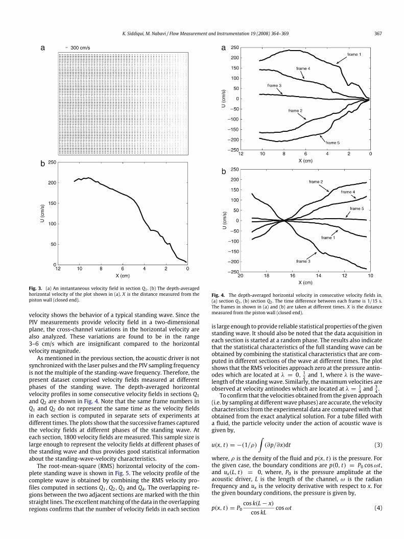
An instantaneous two-dimensional velocity field in the regionadjacent to the piston (i.e. sectionQ1) is shown in Fig. 3(a). The plotshows that the velocity magnitude decreases when approachingthe piston and becomes almost zero immediately adjacent to thepiston. This is an expected behavior as the pressure fluctuationsare maximum at the piston (i.e. pressure antinode). Moving fromright to left in the plot, the velocity increases up to a certaindistance and then starts decreasing. The maximum velocity occursat the location where the pressure fluctuations are minimum. Inthe present figure, the maximum velocity is located at 8.25 cmfrom the piston end. The depth-averaged horizontal velocity ofthe velocity field in Fig. 3(a) is shown in Fig. 3(b). The horizontal

K. Siddiqui, M. Nabavi / Flow Measurement and Instrumentation 19 (2008) 364–369 367

Fig. 3. (a) An instantaneous velocity field in section Q1 . (b) The depth-averagedhorizontal velocity of the plot shown in (a). X is the distance measured from thepiston wall (closed end).

velocity shows the behavior of a typical standing wave. Since thePIV measurements provide velocity field in a two-dimensionalplane, the cross-channel variations in the horizontal velocity arealso analyzed. These variations are found to be in the range3–6 cm/s which are insignificant compared to the horizontalvelocity magnitude.As mentioned in the previous section, the acoustic driver is not

synchronizedwith the laser pulses and the PIV sampling frequencyis not the multiple of the standing-wave frequency. Therefore, thepresent dataset comprised velocity fields measured at differentphases of the standing wave. The depth-averaged horizontalvelocity profiles in some consecutive velocity fields in sections Q1and Q2 are shown in Fig. 4. Note that the same frame numbers inQ1 and Q2 do not represent the same time as the velocity fieldsin each section is computed in separate sets of experiments atdifferent times. The plots show that the successive frames capturedthe velocity fields at different phases of the standing wave. Ateach section, 1800 velocity fields are measured. This sample size islarge enough to represent the velocity fields at different phases ofthe standing wave and thus provides good statistical informationabout the standing-wave-velocity characteristics.The root-mean-square (RMS) horizontal velocity of the com-

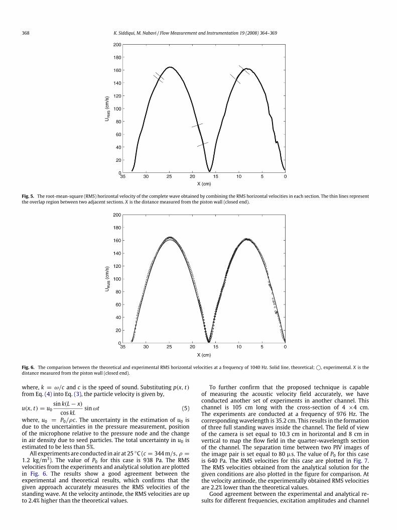
plete standing wave is shown in Fig. 5. The velocity profile of thecomplete wave is obtained by combining the RMS velocity pro-files computed in sections Q1,Q2,Q3 and Q4. The overlapping re-gions between the two adjacent sections are marked with the thinstraight lines. The excellentmatching of the data in the overlappingregions confirms that the number of velocity fields in each section

Fig. 4. The depth-averaged horizontal velocity in consecutive velocity fields in,(a) section Q1 , (b) section Q2 . The time difference between each frame is 1/15 s.The frames in shown in (a) and (b) are taken at different times. X is the distancemeasured from the piston wall (closed end).

is large enough to provide reliable statistical properties of the givenstanding wave. It should also be noted that the data acquisition ineach section is started at a random phase. The results also indicatethat the statistical characteristics of the full standing wave can beobtained by combining the statistical characteristics that are com-puted in different sections of the wave at different times. The plotshows that the RMS velocities approach zero at the pressure antin-odes which are located at λ = 0, 12 and 1, where λ is the wave-length of the standingwave. Similarly, themaximum velocities areobserved at velocity antinodes which are located at λ = 1

4 and34 .

To confirm that the velocities obtained from the given approach(i.e. by sampling at differentwavephases) are accurate, the velocitycharacteristics from the experimental data are comparedwith thatobtained from the exact analytical solution. For a tube filled witha fluid, the particle velocity under the action of acoustic wave isgiven by,

u(x, t) = −(1/ρ)∫(∂p/∂x)dt (3)

where, ρ is the density of the fluid and p(x, t) is the pressure. Forthe given case, the boundary conditions are p(0, t) = P0 cosωt ,and ux(L, t) = 0, where, P0 is the pressure amplitude at theacoustic driver, L is the length of the channel, ω is the radianfrequency and ux is the velocity derivative with respect to x. Forthe given boundary conditions, the pressure is given by,

p(x, t) = P0cos k(L− x)cos kL

cosωt (4)

368 K. Siddiqui, M. Nabavi / Flow Measurement and Instrumentation 19 (2008) 364–369

Fig. 5. The root-mean-square (RMS) horizontal velocity of the complete wave obtained by combining the RMS horizontal velocities in each section. The thin lines representthe overlap region between two adjacent sections. X is the distance measured from the piston wall (closed end).

Fig. 6. The comparison between the theoretical and experimental RMS horizontal velocities at a frequency of 1040 Hz. Solid line, theoretical;©, experimental. X is thedistance measured from the piston wall (closed end).

where, k = ω/c and c is the speed of sound. Substituting p(x, t)from Eq. (4) into Eq. (3), the particle velocity is given by,

u(x, t) = u0sin k(L− x)cos kL

sinωt (5)

where, u0 = P0/ρc. The uncertainty in the estimation of u0 isdue to the uncertainties in the pressure measurement, positionof the microphone relative to the pressure node and the changein air density due to seed particles. The total uncertainty in u0 isestimated to be less than 5%.All experiments are conducted in air at 25 ◦C (c = 344m/s, ρ =

1.2 kg/m3). The value of P0 for this case is 938 Pa. The RMSvelocities from the experiments and analytical solution are plottedin Fig. 6. The results show a good agreement between theexperimental and theoretical results, which confirms that thegiven approach accurately measures the RMS velocities of thestanding wave. At the velocity antinode, the RMS velocities are upto 2.4% higher than the theoretical values.

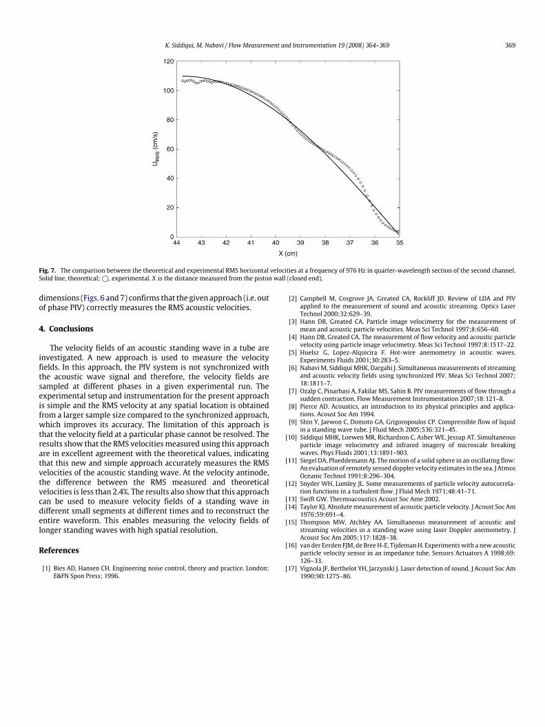
To further confirm that the proposed technique is capableof measuring the acoustic velocity field accurately, we haveconducted another set of experiments in another channel. Thischannel is 105 cm long with the cross-section of 4 ×4 cm.The experiments are conducted at a frequency of 976 Hz. Thecorrespondingwavelength is 35.2 cm. This results in the formationof three full standing waves inside the channel. The field of viewof the camera is set equal to 10.3 cm in horizontal and 8 cm invertical to map the flow field in the quarter-wavelength sectionof the channel. The separation time between two PIV images ofthe image pair is set equal to 80 µs. The value of P0 for this caseis 640 Pa. The RMS velocities for this case are plotted in Fig. 7.The RMS velocities obtained from the analytical solution for thegiven conditions are also plotted in the figure for comparison. Atthe velocity antinode, the experimentally obtained RMS velocitiesare 2.2% lower than the theoretical values.Good agreement between the experimental and analytical re-

sults for different frequencies, excitation amplitudes and channel

K. Siddiqui, M. Nabavi / Flow Measurement and Instrumentation 19 (2008) 364–369 369

Fig. 7. The comparison between the theoretical and experimental RMS horizontal velocities at a frequency of 976 Hz in quarter-wavelength section of the second channel.Solid line, theoretical;©, experimental. X is the distance measured from the piston wall (closed end).

dimensions (Figs. 6 and7) confirms that the given approach (i.e. outof phase PIV) correctly measures the RMS acoustic velocities.

4. Conclusions

The velocity fields of an acoustic standing wave in a tube areinvestigated. A new approach is used to measure the velocityfields. In this approach, the PIV system is not synchronized withthe acoustic wave signal and therefore, the velocity fields aresampled at different phases in a given experimental run. Theexperimental setup and instrumentation for the present approachis simple and the RMS velocity at any spatial location is obtainedfrom a larger sample size compared to the synchronized approach,which improves its accuracy. The limitation of this approach isthat the velocity field at a particular phase cannot be resolved. Theresults show that the RMS velocitiesmeasured using this approachare in excellent agreement with the theoretical values, indicatingthat this new and simple approach accurately measures the RMSvelocities of the acoustic standing wave. At the velocity antinode,the difference between the RMS measured and theoreticalvelocities is less than 2.4%. The results also show that this approachcan be used to measure velocity fields of a standing wave indifferent small segments at different times and to reconstruct theentire waveform. This enables measuring the velocity fields oflonger standing waves with high spatial resolution.

References

[1] Bies AD, Hansen CH. Engineering noise control, theory and practice. London:E&FN Spon Press; 1996.

[2] Campbell M, Cosgrove JA, Greated CA, Rockliff JD. Review of LDA and PIVapplied to the measurement of sound and acoustic streaming. Optics LaserTechnol 2000;32:629–39.

[3] Hann DB, Greated CA. Particle image velocimetry for the measurement ofmean and acoustic particle velocities. Meas Sci Technol 1997;8:656–60.

[4] Hann DB, Greated CA. The measurement of flow velocity and acoustic particlevelocity using particle image velocimetry. Meas Sci Technol 1997;8:1517–22.

[5] Huelsz G, Lopez-Alquicira F. Hot-wire anemometry in acoustic waves.Experiments Fluids 2001;30:283–5.

[6] Nabavi M, Siddiqui MHK, Dargahi J. Simultaneousmeasurements of streamingand acoustic velocity fields using synchronized PIV. Meas Sci Technol 2007;18:1811–7.

[7] Ozalp C, Pinarbasi A, Fakilar MS, Sahin B. PIV measurements of flow through asudden contraction. Flow Measurement Instrumentation 2007;18:121–8.

[8] Pierce AD. Acoustics, an introduction to its physical principles and applica-tions. Acoust Soc Am 1994.

[9] Shin Y, Jaewon C, Domoto GA, Grigoropoulos CP. Compressible flow of liquidin a standing wave tube. J Fluid Mech 2005;536:321–45.

[10] Siddiqui MHK, Loewen MR, Richardson C, Asher WE, Jessup AT. Simultaneousparticle image velocimetry and infrared imagery of microscale breakingwaves. Phys Fluids 2001;13:1891–903.

[11] Siegel DA, Plueddemann AJ. Themotion of a solid sphere in an oscillating flow:An evaluation of remotely senseddoppler velocity estimates in the sea. J AtmosOceanic Technol 1991;8:296–304.

[12] Snyder WH, Lumley JL. Some measurements of particle velocity autocorrela-tion functions in a turbulent flow. J Fluid Mech 1971;48:41–71.

[13] Swift GW. Thermoacoustics Acoust Soc Ame 2002.[14] Taylor KJ. Absolutemeasurement of acoustic particle velocity. J Acoust Soc Am

1976;59:691–4.[15] Thompson MW, Atchley AA. Simultaneous measurement of acoustic and

streaming velocities in a standing wave using laser Doppler anemometry. JAcoust Soc Am 2005;117:1828–38.

[16] van der Eerden FJM, de BreeH-E, TijdemanH. Experimentswith a newacousticparticle velocity sensor in an impedance tube. Sensors Actuators A 1998;69:126–33.

[17] Vignola JF, Berthelot YH, Jarzynski J. Laser detection of sound. J Acoust Soc Am1990;90:1275–86.