Mean-Variance Analysis versus Full-Scale Optimization

Revere Street Working Paper Series

Financial Economics 272-18

Mean-Variance Analysis versus Full-Scale Optimization -

Out of Sample

First Version: November 11, 2005 This Draft: December 13, 2005

Timothy Adler Mark Kritzman Windham Capital Management, LLC Windham Capital Management, LLC 5 Revere Street 5 Revere Street Cambridge, MA 02138 Cambridge, MA 02138 617 234-9459 617 576-7360 [email protected] [email protected]

Abstract

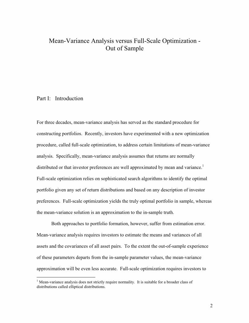
For three decades, mean-variance analysis has served as the standard procedure for constructing portfolios. Recently, investors have experimented with a new optimization procedure, called full-scale optimization, to address certain limitations of mean-variance optimization. Specifically, mean-variance optimization assumes that returns are normally distributed or that investor preferences are well approximated by mean and variance. Full-scale optimization relies on sophisticated search algorithms to identify the optimal portfolio given any set of return distributions and based on any description of investor preferences. Full-scale optimization yields the truly optimal portfolio in sample, whereas the mean-variance solution is an approximation to the in-sample truth. Both approaches to portfolio formation, however, suffer from estimation error. Mean-variance analysis requires investors to estimate the means and variances of all assets and the covariances of all asset pairs. To the extent the out-of-sample experience of these parameters departs from the in-sample parameter values, the mean-variance approximation will be even less accurate. Full-scale optimization requires investors to estimate the entire multivariate return distribution. To the extent it varies from the in-sample distribution, full-scale optimization will also yield sub-optimal results out of sample. We employ a bootstrapping procedure to compare the estimation error of full-scale optimization to the combined approximation and estimation error of mean-variance analysis. We find that, to a significant degree, the in-sample superiority of full-scale optimization prevails out-of-sample.

2

Mean-Variance Analysis versus Full-Scale Optimization -

Out of Sample

Part I: Introduction

For three decades, mean-variance analysis has served as the standard procedure for

constructing portfolios. Recently, investors have experimented with a new optimization

procedure, called full-scale optimization, to address certain limitations of mean-variance

analysis. Specifically, mean-variance analysis assumes that returns are normally

distributed or that investor preferences are well approximated by mean and variance.1

Full-scale optimization relies on sophisticated search algorithms to identify the optimal

portfolio given any set of return distributions and based on any description of investor

preferences. Full-scale optimization yields the truly optimal portfolio in sample, whereas

the mean-variance solution is an approximation to the in-sample truth.

Both approaches to portfolio formation, however, suffer from estimation error.

Mean-variance analysis requires investors to estimate the means and variances of all

assets and the covariances of all asset pairs. To the extent the out-of-sample experience

of these parameters departs from the in-sample parameter values, the mean-variance

approximation will be even less accurate. Full-scale optimization requires investors to

1 Mean-variance analysis does not strictly require normality. It is suitable for a broader class of distributions called elliptical distributions.

3

estimate the entire multivariate return distribution. To the extent it varies from the in-

sample distribution, full-scale optimization will also yield sub-optimal results out of

sample. We employ a bootstrapping procedure to compare the estimation error of full-

scale optimization to the combined approximation and estimation error of mean-variance

analysis. We find that, to a significant degree, the in-sample superiority of full-scale

optimization prevails out-of-sample.

We organize the paper as follows. In Part II we review mean-variance analysis

and its limiting assumptions, and we describe full-scale optimization. In Part III we

review our bootstrapping procedure for generating out-of-sample results. We present

these results in Part IV, and we conclude the paper in Part V.

Part II: Alternative Approaches to Optimization

Mean-Variance Analysis and Its Limitations

In his classic article, "Portfolio Selection" (1952), Markowitz submitted that investors

should not choose portfolios that maximize expected return, because this criterion by

itself ignores the principle of diversification. He proposed that investors should instead

consider variances of returns, along with expected returns, and choose portfolios that

offer the highest expected return for a given level of variance. He called this rule the E-V

maxim.

Markowitz demonstrated that, for given levels of risk, we can identify particular

combinations of securities that maximize expected return. He deemed these portfolios

4

"efficient" and referred to a continuum of such portfolios in dimensions of expected

return and standard deviation as the efficient frontier. According to Markowitz's E-V

maxim, investors should choose portfolios located along the efficient frontier.

This approach to portfolio formation is sufficient for maximizing expected utility

if portfolio returns are normally distributed or if investors have quadratic utility, which is

defined as E(U) = µ – λ σ2, where µ equals portfolio expected return, λ equals risk

aversion, and σ2 equals portfolio variance.2 If returns are normally distributed, investors

can infer the entire distribution of returns from its mean and variance; hence the

irrelevance of specific periodic returns or higher moments. And even if returns are not

normally distributed, quadratic utility assumes that investors are indifferent to other

features of the distribution.

Many assets display return distributions that are approximately normal; however,

no asset produces a perfectly normal distribution. Moreover, quadratic utility is not a

realistic description of a typical investor’s attitude toward risk, because it assumes that

investors are as averse to upside deviations as they are to downside deviations and that at

certain wealth levels they prefer less wealth to more wealth.

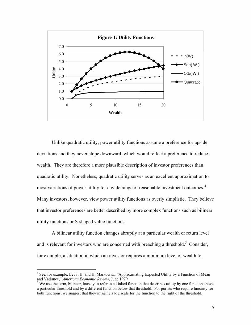
Financial economists usually assume that investors have power utility functions,

which define utility as 1/γ x Wealthγ. A log wealth utility function is a special case of

power utility. As γ approaches 0, utility approaches the natural logarithm of wealth. A γ

equal to ½ implies less risk aversion than log wealth, while a γ equal to -1 implies greater

risk aversion.3 These utility functions, along with a quadratic utility function, are shown

in Figure 1.

2 Mean-variance analysis is also suitable for a broader class of distributions called elliptical distributions. 3 When γ equals -1, utility is expressed as 1 – W-1.

5

Figure 1: Utility Functions

0.0

1.0

2.0

3.0

4.0

5.0

6.0

7.0

0 5 10 15 20

Wealth

Util

ityln(W)

Sqrt( W )

1-1/( W )

Quadratic

Unlike quadratic utility, power utility functions assume a preference for upside

deviations and they never slope downward, which would reflect a preference to reduce

wealth. They are therefore a more plausible description of investor preferences than

quadratic utility. Nonetheless, quadratic utility serves as an excellent approximation to

most variations of power utility for a wide range of reasonable investment outcomes.4

Many investors, however, view power utility functions as overly simplistic. They believe

that investor preferences are better described by more complex functions such as bilinear

utility functions or S-shaped value functions.

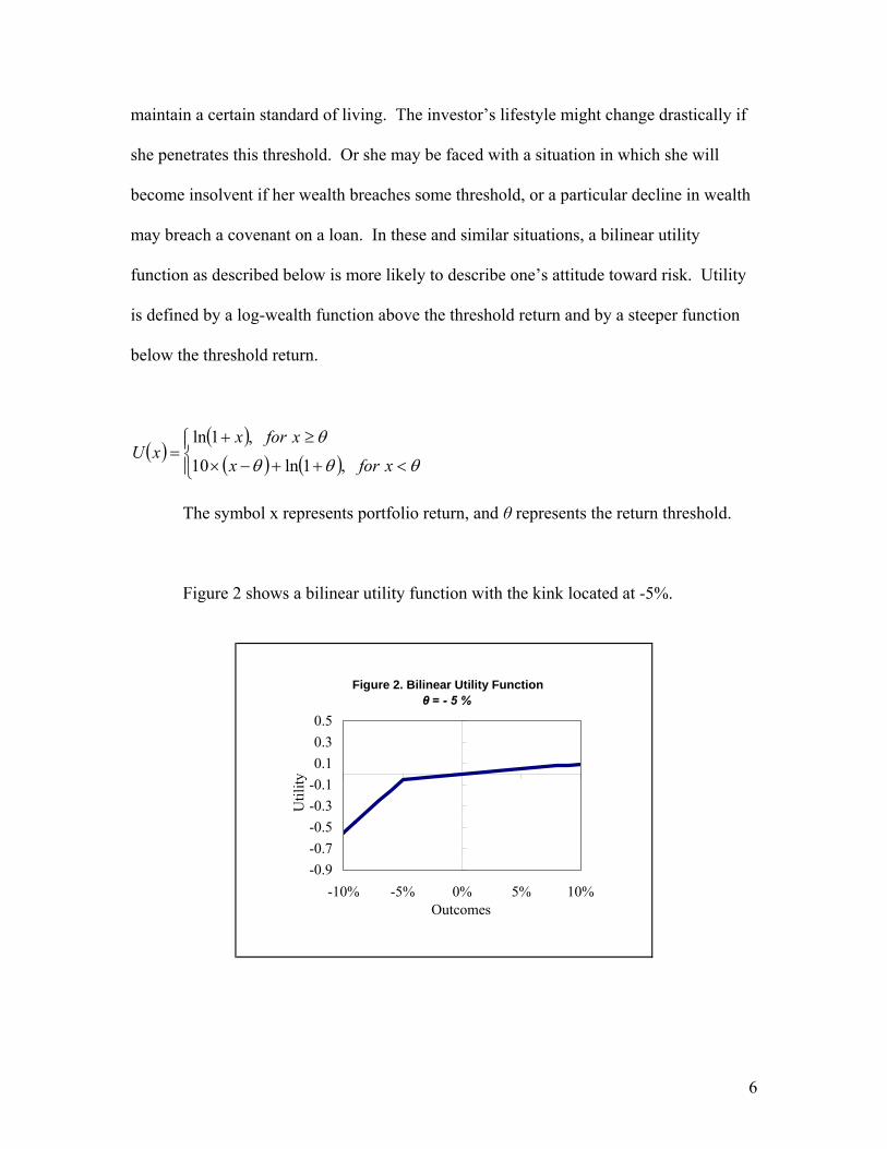
A bilinear utility function changes abruptly at a particular wealth or return level

and is relevant for investors who are concerned with breaching a threshold.5 Consider,

for example, a situation in which an investor requires a minimum level of wealth to

4 See, for example, Levy, H. and H. Markowitz. “Approximating Expected Utility by a Function of Mean and Variance,” American Economic Review, June 1979 5 We use the term, bilinear, loosely to refer to a kinked function that describes utility by one function above a particular threshold and by a different function below that threshold. For purists who require linearity for both functions, we suggest that they imagine a log scale for the function to the right of the threshold.

6

maintain a certain standard of living. The investor’s lifestyle might change drastically if

she penetrates this threshold. Or she may be faced with a situation in which she will

become insolvent if her wealth breaches some threshold, or a particular decline in wealth

may breach a covenant on a loan. In these and similar situations, a bilinear utility

function as described below is more likely to describe one’s attitude toward risk. Utility

is defined by a log-wealth function above the threshold return and by a steeper function

below the threshold return.

( )( )( ) ( )⎪⎩

⎪⎨⎧

<++−×

≥+=

θθθ

θ

xforx

xforxxU

,1ln10

,1ln

The symbol x represents portfolio return, and θ represents the return threshold.

Figure 2 shows a bilinear utility function with the kink located at -5%.

Figure 2. Bilinear Utility Functionθ = - 5 %

-0.9-0.7-0.5-0.3-0.10.10.30.5

-10% -5% 0% 5% 10%Outcomes

Util

ity

7

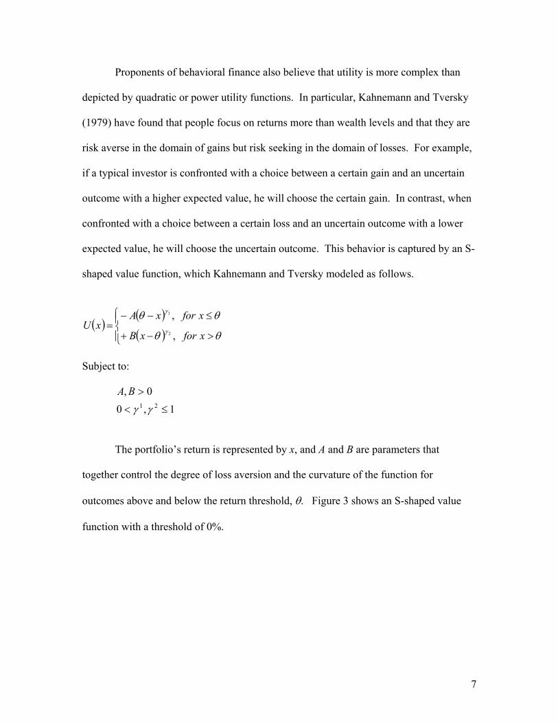
Proponents of behavioral finance also believe that utility is more complex than

depicted by quadratic or power utility functions. In particular, Kahnemann and Tversky

(1979) have found that people focus on returns more than wealth levels and that they are

risk averse in the domain of gains but risk seeking in the domain of losses. For example,

if a typical investor is confronted with a choice between a certain gain and an uncertain

outcome with a higher expected value, he will choose the certain gain. In contrast, when

confronted with a choice between a certain loss and an uncertain outcome with a lower

expected value, he will choose the uncertain outcome. This behavior is captured by an S-

shaped value function, which Kahnemann and Tversky modeled as follows.

( )( )( )⎪⎩

⎪⎨⎧

>−+

≤−−=

θθ

θθγ

γ

xforxB

xforxAxU

,

,2

1

Subject to:

1,00,

21 ≤<

>

γγ

BA

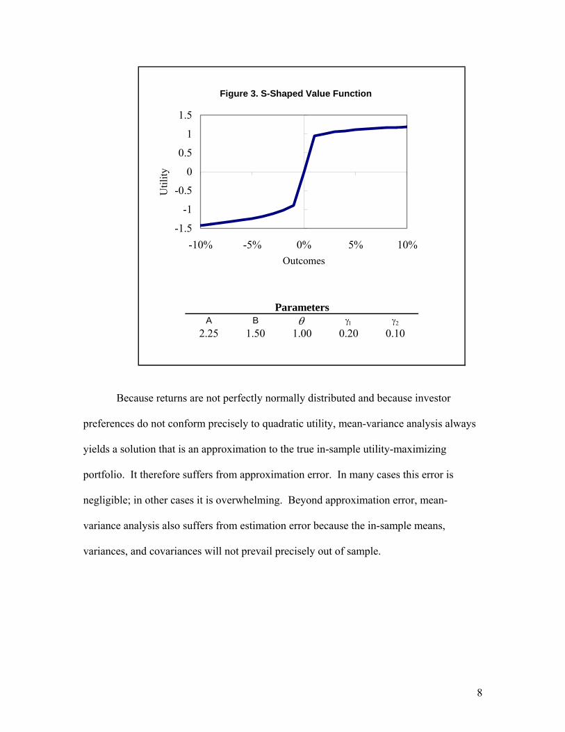
The portfolio’s return is represented by x, and A and B are parameters that

together control the degree of loss aversion and the curvature of the function for

outcomes above and below the return threshold, θ. Figure 3 shows an S-shaped value

function with a threshold of 0%.

8

A B θ γ1 γ22.25 1.50 1.00 0.20 0.10

Parameters

Figure 3. S-Shaped Value Function

-1.5

-1

-0.5

0

0.5

1

1.5

-10% -5% 0% 5% 10%Outcomes

Util

ity

1

Because returns are not perfectly normally distributed and because investor

preferences do not conform precisely to quadratic utility, mean-variance analysis always

yields a solution that is an approximation to the true in-sample utility-maximizing

portfolio. It therefore suffers from approximation error. In many cases this error is

negligible; in other cases it is overwhelming. Beyond approximation error, mean-

variance analysis also suffers from estimation error because the in-sample means,

variances, and covariances will not prevail precisely out of sample.

9

Full-Scale Optimization

Computational efficiency now allows us to perform full-scale optimization as an

alternative to mean-variance analysis. With this approach we calculate a portfolio’s

utility for every period in our sample, considering as many asset mixes as necessary to

identify the weights that yield the highest expected utility, given any description of utility

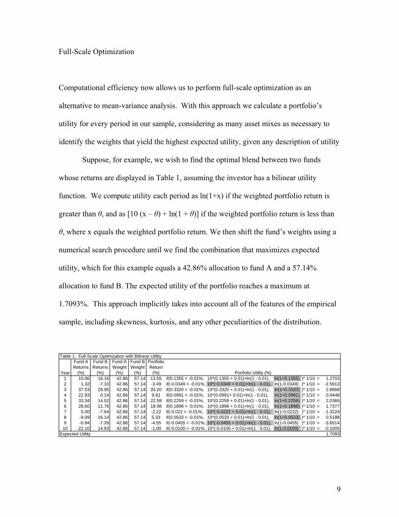
Suppose, for example, we wish to find the optimal blend between two funds

whose returns are displayed in Table 1, assuming the investor has a bilinear utility

function. We compute utility each period as ln(1+x) if the weighted portfolio return is

greater than θ, and as [10 (x – θ) + ln(1 + θ)] if the weighted portfolio return is less than

θ, where x equals the weighted portfolio return. We then shift the fund’s weights using a

numerical search procedure until we find the combination that maximizes expected

utility, which for this example equals a 42.86% allocation to fund A and a 57.14%

allocation to fund B. The expected utility of the portfolio reaches a maximum at

1.7093%. This approach implicitly takes into account all of the features of the empirical

sample, including skewness, kurtosis, and any other peculiarities of the distribution.

Table 1: Full-Scale Optimization with Bilinear Utility

Year

Fund A Returns

(%)

Fund B Returns

(%)

Fund A Weight

(%)

Fund B Weight

(%)

Portfolio Return

(%) Portfolio Utility (%)1 10.06 16.16 42.86 57.14 13.55 if(0.1355 < -0.01%, 10*(0.1355 + 0.01)+ln(1 - 0.01), ln(1+0.1355) )* 1/10 = 1.27032 1.32 -7.10 42.86 57.14 -3.49 if(-0.0349 < -0.01%, 10*(-0.0349 + 0.01)+ln(1 - 0.01), ln(1-0.0349) )* 1/10 = -2.59133 37.53 29.95 42.86 57.14 33.20 if(0.3320 < -0.01%, 10*(0.3320 + 0.01)+ln(1 - 0.01), ln(1+0.3320) )* 1/10 = 2.86684 22.93 0.14 42.86 57.14 9.91 if(0.0991 < -0.01%, 10*(0.0991+ 0.01)+ln(1 - 0.01), ln(1+0.0991) )* 1/10 = 0.94485 33.34 14.52 42.86 57.14 22.59 if(0.2259 < -0.01%, 10*(0.2259 + 0.01)+ln(1 - 0.01), ln(1+0.2259) )* 1/10 = 2.03656 28.60 11.76 42.86 57.14 18.98 if(0.1898 < -0.01%, 10*(0.1898 + 0.01)+ln(1 - 0.01), ln(1+0.1898) )* 1/10 = 1.73777 5.00 -7.64 42.86 57.14 -2.22 if(-0.022 < -0.01%, 10*(-0.0222 + 0.01)+ln(1 - 0.01), ln(1-0.0222) )* 1/10 = -1.32248 -9.09 16.14 42.86 57.14 5.33 if(0.0533 < -0.01%, 10*(0.0533 + 0.01)+ln(1 - 0.01), ln(1+0.0533) )* 1/10 = 0.51889 -0.94 -7.26 42.86 57.14 -4.55 if(-0.0455 < -0.01%, 10*(-0.0455 + 0.01)+ln(1 - 0.01), ln(1-0.0455) )* 1/10 = -3.6514

10 -22.10 14.83 42.86 57.14 -1.00 if(-0.0100 < -0.01%, 10*(-0.0100 + 0.01)+ln(1 - 0.01), ln(1-0.0100) )* 1/10 = -0.1005Expected Utility 1.7093

10

We can apply full-scale optimization to empirical distributions, theoretical

distributions, or combinations based on empirical returns and theoretical assumptions. If

we assume a theoretical distribution, we simply discretize it by randomly drawing returns

from it and then applying the full-scale algorithm to these discrete returns. If we prefer to

preserve the shape of an empirical sample but modify the assets’ means to conform with

our views about them prospectively, we simply adjust each return in the empirical sample

by the difference between our view and the empirical mean.

Assuming our search algorithm is sufficiently powerful, full-scale optimization

will yield the true in-sample utility-maximizing portfolio. Unlike mean-variance

analysis, it has no approximation error. However, like mean-variance analysis it too

suffers from estimation error. To the extent any of the features of the in-sample

distribution do not prevail out of sample, the full-scale solution will be sub-optimal. In

the next section we describe the methodology we use to compare the combination of

approximation and estimation error of mean-variance analysis to the estimation error of

full-scale optimization.

Part III: Methodology

We base our analysis on a sample of monthly hedge fund returns covering a 10-year

period from January 1995 through December 2004. We selected this sample because

11

hedge funds tend to display significantly non-normal higher moments6. In order to

mitigate the effect of selection bias in the hedge fund sample, we scale each return to

conform to expected returns that are proportional to the implied returns of an equally

weighted portfolio.

We consider four utility functions: bilinear with the kink set at -1%; bilinear with

the kink set at -5%; S-shaped with the inflection point set at 0%; and S-shaped with the

inflection point set at 0.5%. We do not consider any power utility functions because the

approximation errors of mean-variance analysis are arbitrarily small for these utility

functions.7

We begin by solving for the in-sample utility-maximizing portfolio using our full-

scale optimization algorithm. Then we solve for the mean-variance portfolio on the

efficient frontier that has the same expected return as the full-scale optimal portfolio. We

record the asset weights of these portfolios, as well as their expected utility, expected

return, standard deviation, kurtosis, and skewness.

We next bootstrap one-month vectors of cross-sectional returns with replacement

12 times to generate a new one-year sample of returns. We repeat this procedure until we

have 1,000 new one-year samples. Next we apply the weights that we generated from

our full-scale optimization and mean-variance analysis of the original 10-year return

sample, and we apply these weights to the new 1,000 annual samples. We then compute

the portfolio metrics of these 1,000 out-of -sample histories.

6 See, for example, Alexiev, J. 2004. “The Impact of Higher Moments on Hedge Fund Risk Exposure.” Journal of Alternative Investments. Spring 2005 7 See, for example, Cremers, J-H, M’ Kritzman, and S. Page, “Optimal Hedge Fund Allocations,” The Journal of Portfolio Management, Spring 2005

12

We perform two additional bootstrap exercises in which we generate 1,000 five-

year and 10-year samples. Again, we apply the weights from the in-sample full-scale and

mean-variance optimizations to these new return samples and compute the portfolio

metrics of these five and 10-year out-of-sample histories.

These results allow us to compare how well the full-scale and mean-variance

weights derived in sample perform out of sample. In the case of the full-scale optimal

portfolios, the differences from the in-sample results arise purely from estimation error.

In the case of the mean-variance portfolios, the differences arise from a combination of

approximation and estimation error.

13

Part IV: Results

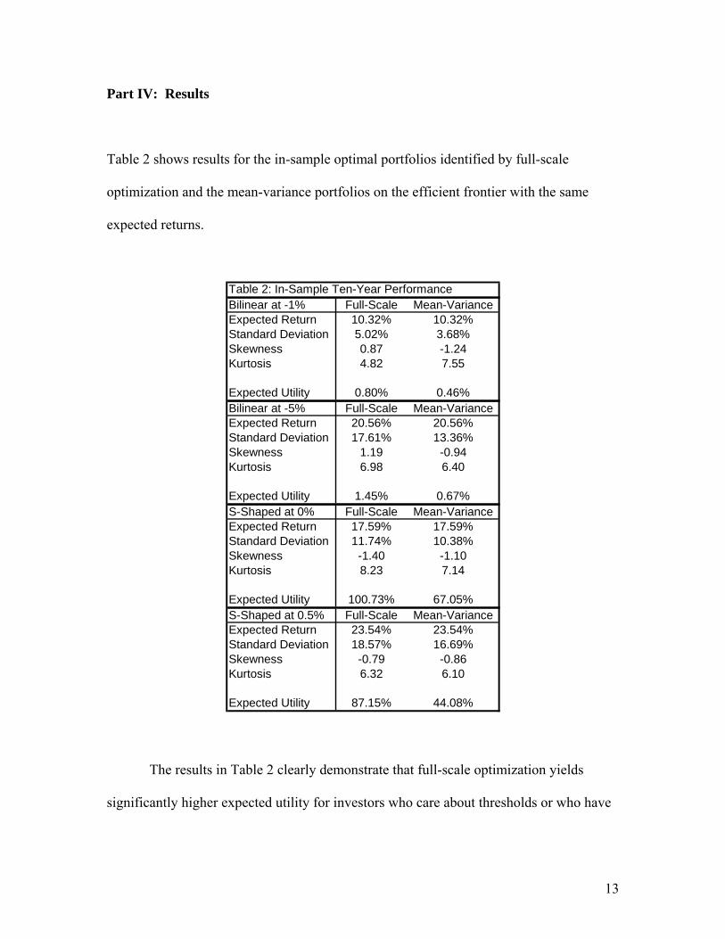
Table 2 shows results for the in-sample optimal portfolios identified by full-scale

optimization and the mean-variance portfolios on the efficient frontier with the same

expected returns.

Table 2: In-Sample Ten-Year PerformanceBilinear at -1% Full-Scale Mean-VarianceExpected Return 10.32% 10.32%Standard Deviation 5.02% 3.68%Skewness 0.87 -1.24Kurtosis 4.82 7.55

Expected Utility 0.80% 0.46%Bilinear at -5% Full-Scale Mean-VarianceExpected Return 20.56% 20.56%Standard Deviation 17.61% 13.36%Skewness 1.19 -0.94Kurtosis 6.98 6.40

Expected Utility 1.45% 0.67%S-Shaped at 0% Full-Scale Mean-VarianceExpected Return 17.59% 17.59%Standard Deviation 11.74% 10.38%Skewness -1.40 -1.10Kurtosis 8.23 7.14

Expected Utility 100.73% 67.05%S-Shaped at 0.5% Full-Scale Mean-VarianceExpected Return 23.54% 23.54%Standard Deviation 18.57% 16.69%Skewness -0.79 -0.86Kurtosis 6.32 6.10

Expected Utility 87.15% 44.08%

The results in Table 2 clearly demonstrate that full-scale optimization yields

significantly higher expected utility for investors who care about thresholds or who have

14

different preferences with respect to gains and losses. These differences arise entirely

from the approximation error of mean-variance analysis.

The first panel shows the results assuming a bilinear utility function with the kink

located at a -1% return. It reveals that the full-scale optimization generates higher

expected utility than mean-variance analysis. It also reveals that the full-scale portfolios

display less kurtosis and less negative skewness than the mean-variance portfolios,

characteristics that are undesirable to investors with bilinear utility. The same pattern

prevails in the second panel, which assumes the kink is located at a -5% return.

The third panel assumes an S-Shaped function with the inflection point located at

a 0% return. Again, the full-scale portfolios perform better than the mean-variance

portfolios as evidenced by their higher expected utility. It also reveals that the full-scale

optimization produces more negative skewness than mean-variance analysis. S-Shaped

investors are not attracted to extremely bad outcomes; they just do not especially mind

them. They are, however, strongly attracted to the high density of moderately good

outcomes, which serves as the offset to the few extremely bad outcomes in a negatively

skewed distribution. Full-scale optimization does an excellent job of accommodating

these preferences, while mean-variance analysis ignores them. This pattern prevails in

the fourth panel, which assumes S-Shaped utility with the inflection point located at a

0.5% return

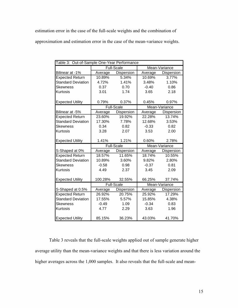
Next we show the extent to which the in-sample superiority of the full-scale

weights prevails out of sample. Table 3 shows performance of the in-sample full-scale

and mean-variance weights for the bootstrapped one-year samples. The differences we

observe between the out-of-sample results and the in-sample full-scale results arise from

15

estimation error in the case of the full-scale weights and the combination of

approximation and estimation error in the case of the mean-variance weights.

Table 3: Out-of-Sample One-Year Performance

Average Dispersion Average Dispersion Expected Return 10.89% 5.34% 10.69% 3.77%Standard Deviation 4.72% 1.41% 3.48% 1.10%Skewness 0.37 0.70 -0.40 0.86Kurtosis 3.01 1.74 3.65 2.18

Expected Utility 0.79% 0.37% 0.45% 0.97%

Bilinear at -5% Average Dispersion Average DispersionExpected Return 23.60% 19.92% 22.28% 13.74%Standard Deviation 17.30% 7.78% 12.68% 3.53%Skewness 0.34 0.82 -0.33 0.82Kurtosis 3.28 2.07 3.53 2.00


S-Shaped at 0% Average Dispersion Average Dispersion Expected Return 18.57% 11.65% 18.74% 10.55%Standard Deviation 10.89% 3.60% 9.82% 2.80%Skewness -0.58 0.98 -0.37 0.81Kurtosis 4.49 2.37 3.45 2.09


S-Shaped at 0.5% Average Dispersion Average Dispersion Expected Return 26.92% 20.75% 25.92% 17.29%Standard Deviation 17.55% 5.57% 15.85% 4.38%Skewness -0.49 1.09 -0.34 0.83Kurtosis 4.77 2.29 3.63 1.96


Bilinear at -1%

Full-Scale Mean-Variance




Table 3 reveals that the full-scale weights applied out of sample generate higher

average utility than the mean-variance weights and that there is less variation around the

higher averages across the 1,000 samples. It also reveals that the full-scale and mean-

16

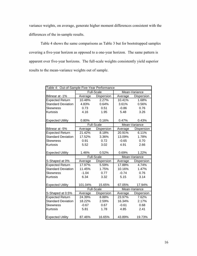
variance weights, on average, generate higher moment differences consistent with the

differences of the in-sample results.

Table 4 shows the same comparisons as Table 3 but for bootstrapped samples

covering a five-year horizon as opposed to a one-year horizon. The same pattern is

apparent over five-year horizons. The full-scale weights consistently yield superior

results to the mean-variance weights out of sample.

Table 4: Out-of-Sample Five-Year Performance









Bilinear at -1%





17

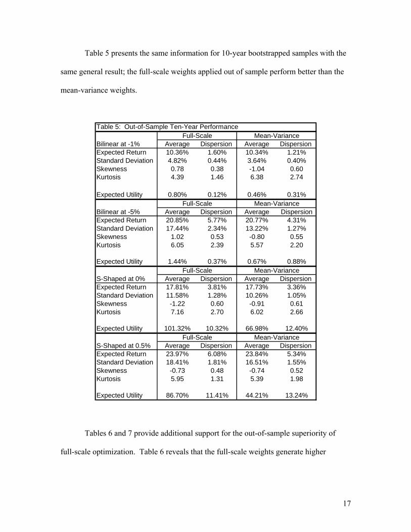
Table 5 presents the same information for 10-year bootstrapped samples with the

same general result; the full-scale weights applied out of sample perform better than the

mean-variance weights.

Table 5: Out-of-Sample Ten-Year Performance









Bilinear at -1%





Tables 6 and 7 provide additional support for the out-of-sample superiority of

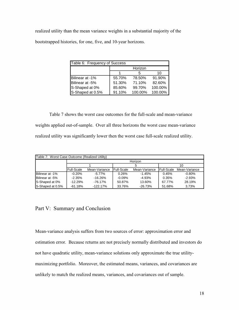
full-scale optimization. Table 6 reveals that the full-scale weights generate higher

18

realized utility than the mean variance weights in a substantial majority of the

bootstrapped histories, for one, five, and 10-year horizons.

Table 6: Frequency of Success

1 5 10Bilinear at -1% 55.70% 78.50% 91.90%Bilinear at -5% 51.30% 71.10% 82.60%S-Shaped at 0% 85.60% 99.70% 100.00%S-Shaped at 0.5% 91.10% 100.00% 100.00%

Horizon

Table 7 shows the worst case outcomes for the full-scale and mean-variance

weights applied out-of-sample. Over all three horizons the worst case mean-variance

realized utility was significantly lower then the worst case full-scale realized utility.

Table 7: Worst Case Outcome (Realized Utility)

Full-Scale Mean-Variance Full-Scale Mean-Variance Full-Scale Mean-VarianceBilinear at -1% -0.20% -5.77% 0.26% -1.45% 0.45% -0.80%Bilinear at -5% -2.35% -16.26% -0.09% -4.93% 0.35% -2.93%S-Shaped at 0% -12.29% -76.17% 50.87% 13.60% 67.77% 28.19%S-Shaped at 0.5% -61.18% -122.17% 33.76% -26.73% 51.68% 3.73%

Horizon1 5 10

Part V: Summary and Conclusion

Mean-variance analysis suffers from two sources of error: approximation error and

estimation error. Because returns are not precisely normally distributed and investors do

not have quadratic utility, mean-variance solutions only approximate the true utility-

maximizing portfolio. Moreover, the estimated means, variances, and covariances are

unlikely to match the realized means, variances, and covariances out of sample.

19

Full-scale optimization serves as an alternative to mean-variance analysis. It

relies on sophisticated search algorithms to identify the in-sample utility-maximizing

portfolio given any empirical or theoretical return distribution and any description of

investor utility. Therefore, it is not subject to approximation error. Yet it does suffer

from estimation error, because the in-sample distribution of returns will not prevail

precisely out of sample.

We bootstrap an empirical sample of returns to generate thousands of alternative

histories for one, five, and ten-year horizons. We then apply the in-sample weights from

mean-variance analysis and full-scale optimization to the bootstrapped samples to

evaluate their out-of-sample robustness. Our results reveal that the full-scale portfolios

consistently outperform the mean-variance portfolios out of sample; hence the combined

approximation and estimation error of mean-variance analysis is more detrimental to out-

of-sample performance than the estimation error of full-scale optimization.

We feel obliged to add some precautionary comments. We chose a sample of

returns that is significantly non-normal, and we assumed a set of utility functions that,

while perhaps realistic, are unconventional. If instead we used returns that were more

normally distributed, or we based our analysis on variations of power utility, we would

unlikely observe significant approximation error from mean-variance analysis, and the

out-of sample performance of mean-variance analysis and full-scale optimization would

probably be indistinguishable.

Also, our research design implicitly assumes that the empirical distribution we

used to generate our in-sample portfolios accurately characterizes the unobservable

population of returns for these funds and that estimation error is a function of the

20

sampling process. If the empirical sample differs substantively from the unobservable

population – for example, if these returns are truly normally distributed – then our results

would be less interesting. It is therefore important to understand qualitatively why we

should expect a particular distribution from an asset or investment fund. In the case of

hedge funds, there are compelling reasons to expect the non-normal higher moments that

we observe in the empirical sample. See, for example, Davies and Kat (2003), Fung and

Hsieh (2000), Gregoriou and Gueyie (2003), Kat and Lu ((2002), Lo (2001), Lo (2005),

and McFall (2003).

It has already been shown that full-scale optimization offers a better expected

solution than mean-variance analysis for investors with special preferences who invest in

assets with significantly non-normal distributions. Our results show that the superior in-

sample performance of full-scale optimization prevails out-of-sample as well.

21

References

Agarwal, V. and N. Y. Naik. 2000. “Does Gain-Loss Analysis Outperform Mean-Variance Analysis? Evidence from Portfolios of Hedge Funds and Passive Strategies.” IFA Working Paper, London Business School.

Agarwal, V. and N. Y. Naik. 2003. “Risks and Portfolio Decisions Involving Hedge Funds.” Working Paper, London Business School.

Alexiev, J. 2004. “The Impact of Higher Moments on Hedge Fund Risk Exposure.” Journal of Alternative Investments. Spring 2005, pg. 50-65.

Berkelaar, A. and R. Kouwenberg. 2000. “Optimal Portfolio Choice Under Loss Aversion” Econometric Institute Report, Working Paper, EI 2000-08 /A.

Brooks, C. and H. M. Kat. 2002. “The Statistical Properties of Hedge Fund Return Index Returns and Their Implications for Investors.” Journal of Alternative Investments, vol. 5: 26-44. Cremers, J-H, M. Kritzman, and S. Page. “Portfolio Formation with Higher Moments and Plausible Utility.” Revere Street Working Paper Series, Financial Economics 272-12, November 22, 2003. Cremers, J-H, M. Kritzman, and S. Page. “Optimal Hedge Fund Allocations: Do Higher Moments matter?” The Journal of Portfolio Management, Spring 2005.

Cvitanic, J., A. Lazrak, L. Martellini, and F. Zapatero. 2003. “Optimal Allocation to Hedge Funds: An Empirical Analysis.” Quantitative Finance, vol. 3:1-12.

Davies, R. J., H M. Kat, and S. Lu. 2003. “Higher Moment Portfolio Analysis with Hedge Funds.” Unpublished working paper.

Favre, L. and A. Signer. 2002. “The Difficulties of Measuring the Benefits of Hedge Funds.” Journal of Alternative Investments, vol. 5, no. 1:31-42.

Favre, L. and J-A. Galeano. 2001. “Hedge Funds Allocation: Case Study of a Swiss Institutional Investor.” Hedgeworld.

Fung, W. and D. Hsieh. 2000. “Performance Characteristics of Hedge Funds and Commodity Funds: Natural versus Spurious Biases.” Journal of Financial and Quantitative Analysis, vol. 35: 291-307.

Gregoriou, G. and J-P. Gueyie. 2003. “Risk-Adjusted Performance of Funds of Hedge Funds Using a Modified Sharpe Ratio.” Journal of Wealth Management, vol. 6, no. 3:77 – 84.

22

Harvey, C.R., Lietchy, J.C., Lietchty, M.W., and P. Muller. 2003. “Portfolio Selection with Higher Moments”, Unpublished working paper, October.

Kahnemann D. and Tversky, A. “Prospect Theory: An Analysis of Decision Under Risk.” Econometrica, 1979, 47, 263-290.

Kat, H. M., and S. Lu. 2002. “An Excursion into the Statistical Properties of Hedge Fund Returns.” Alternative Investment Research Centre Working Paper Series, Working Paper #0016, (May 1, 2002).

Levy, Haim and Harry M. Markowitz. 1979. “Approximating Expected Utility by a Function of Mean and Variance.” American Economic Review, June, Vol. 69, No. 3.

Lhabitant and Learned. 2002. “Hedge Fund Diversification, How Much is Enough?” Journal of Alternative Assets, Winter.

Lo, A. W. 2001. “Risk Management for Hedge Funds: Introduction and Overview.” Financial Analyst Journal, vol. 57:16-33.

Lo, A. W. The Dynamics of the Hedge Fund Industry, The Research Foundation of the CFA Institute, August 2005.

McFall, R. Lamm Jr. 2003. “Asymmetric Returns and Optimal Hedge Fund Portfolios.” Journal of Alternative Investments, vol. 6, no. 2 (Fall): 9–21.

Statman, M. 1999. “Behavioral Finance: Past Battles and Future Engagements.” Financial Analysts Journal, vol. 55, no. 6 (November/December): 18-27.

Documents

Mean-Variance Analysis versus Full-Scale Optimization