Mean annual temperature estimation based on leaf ...ekowalsk/Kowalski.pdfMean annual temperature estimation based on leaf morphology: a test from tropical South America Elizabeth A

Mean annual temperature estimation based on leafmorphology: a test from tropical South America

Elizabeth A. Kowalski �

University of Michigan, Department of Geological Sciences and Museum of Paleontology, 1109 Geddes Avenue, Ann Arbor,MI 48109-1079, USA

Received 20 April 2001; received in revised form 13 June 2002; accepted 19 September 2002

Abstract

Are models that predict mean annual temperature (MAT) from leaf morphology applicable globally? Fifteenmodels that predict MAT from leaf morphology were tested on thirty floral samples from tropical South America todetermine the degree to which models based on published data that are primarily from other regions are applicable tofloras from tropical South America. The models included are based on regional data from North America, SouthAmerica, and Asia. Of the fifteen models tested, five are simple linear regressions, six are multiple linear regressions,two are canonical correspondence analyses, and two are correspondence analyses followed by nearest neighboranalyses. For the seven modern floras with MAT 9 21‡C, every model overestimates MAT. For the 23 modern floraswith MAT s 21‡C, all models produce variable results without a systematic error. The range of average model errorsis 2.7^7.3‡C, while the absolute extremes of error are 0 and 15.1‡C. Average 95% predictive confidence intervals rangefrom 1.6 to 6.9‡C. Predicted MAT falls within the published standard error of the model for 0^67% of the SouthAmerican test floras. Evaluating the seven sites with MAT 9 21‡C separately from the 23 sites with MAT s 21‡Cshows that no equation accurately estimates MAT of the majority of low-temperature sites, but that four equationsaccurately estimate s 50% of high-temperature sites. The results suggest that at least for sites of unknown or highelevation, mean annual temperature of fossil floras from tropical South America may be better predicted from modelsbased on the leaf morphology of tropical South American floras.; 2002 Elsevier Science B.V. All rights reserved.

Keywords: climate prediction; leaf margin; leaf morphology; mean annual temperature; neotropics; South America

1. Introduction

In the eleventh century, Shen Kuo described thepaleoclimate of Shansi Province, China, based onfossil plants that he found in the region (Li, 1981).From this early beginning, the use of fossil £oras

to interpret paleoclimate has become a much-usedtechnique. Modern study of the correlation be-tween paleoclimate and plant fossils, especiallythe morphology of fossil leaves, started in theearly 1900s with an investigation of the relation-ship between climate and extant plants. At thattime, Bailey and Sinnott (1915, 1916) noted thattemperate climates have proportionately morespecies with toothed-margined leaves than dotropical, frigid, or desert climates, and used this

0031-0182 / 02 / $ ^ see front matter ; 2002 Elsevier Science B.V. All rights reserved.PII: S 0 0 3 1 - 0 1 8 2 ( 0 2 ) 0 0 5 5 0 - 3

* Fax: +1-734-936-1380.E-mail address: [email protected] (E.A. Kowalski).

PALAEO 2945 8-11-02

Palaeogeography, Palaeoclimatology, Palaeoecology 188 (2002) 141^165

www.elsevier.com/locate/palaeo

mailto:[email protected]

http://www.elsevier.com/locate/palaeo

qualitative relationship to infer climate from Cre-taceous and Tertiary fossil leaf assemblages.Wolfe (1979) ¢rst quanti¢ed a relationship be-tween leaf margin and temperature using modern£oras from east Asia.

In addition to margin type, other aspects of leafmorphology, such as apex shape and leaf size, arethought to vary based on environmental condi-tions (e.g. Parkhurst and Loucks, 1972; Givnish,1987; Uhl and Mosbrugger, 1999). The relation-ship between leaf morphology and climatic con-ditions is thought to re£ect the convergent adap-tation of leaf form to climate regime (e.g.Parkhurst and Loucks, 1972; Wolfe, 1978; Uhland Mosbrugger, 1999). The same or similar com-binations of characters tend to be common in£oras living in similar climates (Givnish, 1987),even those that are widely separated spatiallyand compositionally (Wolfe, 1978; Halloy andMark, 1996). However, the amount of morpho-logic change is limited in some respects by phy-logeny (Givnish, 1987; Bongers and Popma,1990). Phylogenetic constraints may conserve themorphologic composition of species in any given£ora even when climate changes, and thus therelationship between climate and morphology,should vary geographically based on di¡erencesin taxonomic composition.

Quantifying the modern relationship betweenleaf morphology and climate allows the creationof predictive equations that are used to recon-struct paleoclimate using fossil leaves. Many pub-lished methods detail the relationship between leafmorphology and several di¡erent climatic param-eters, including mean annual temperature (MAT),mean annual precipitation, mean annual range oftemperature, and cold month mean temperature,among others. This paper concentrates on the re-lationship between leaf morphology and MAT.

Four di¡erent methods have been used toquantify the relationship between leaf morphol-ogy and MAT: simple linear regression (SLR),multiple linear regression (MLR), canonical cor-respondence analysis (CCA), and nearest neigh-bor analysis (NN). These four methods are thebasic techniques from which over 20 separateequations, or models, have been constructed.Many published equations that predict MAT

rely on the CLAMP database (Gregory andChase, 1992; Wing and Greenwood, 1993; Greg-ory, 1994; Gregory and McIntosh, 1996; Wilf,1997; Wiemann et al., 1998), a database of mod-ern climate and leaf morphological charactersfrom North America and the Paci¢c compiledby Wolfe (1993, 1995). Other published equationsare derived from data from the Western Hemi-sphere (Wilf, 1997), Bolivia (Gregory-Wodzicki,2000), and eastern Asia (Wolfe, 1978, 1979).While it is reasonable to assume that these equa-tions accurately predict MAT from leaf morphol-ogy in the area from which the data sets are de-rived, the applicability of these models to othergeographical areas is not known.

Many published models that predict MAT havebeen used previously in geographical regions oth-er than the region from which the data set wasderived, with varied results. While some studieshave shown that published equations accuratelypredict MAT of sites from outside the geograph-ical range of that equation’s database (Jacobs andDeino, 1996; Gregory-Wodzicki, 2000; Burnhamet al., 2001), other studies have shown estimatesof MAT that are o¡ by as much as 7‡C (Burn-ham, 1997; Jordan, 1997; Stranks and England,1997; Wiemann et al., 1998), and it has been sug-gested that the relationship between leaf morphol-ogy and temperature is not consistent betweenwidely di¡erent regions (Wolfe, 1995; Green-wood, 2001). Clearly, geographic variation existsin the relationship between climate and leaf mor-phology. Thus, models used to predict MAT fromleaf morphology must be tested using modern re-gional £oras before they are applied to fossil £o-ras from those regions.

Many of the published predictive models maynot accurately estimate MAT in South Americabecause South American sites are poorly repre-sented in the databases used to construct themodels (except Gregory-Wodzicki, 2000). Muchof South America lies within the tropics (Fig. 1),where proportions of entire-margined species arehigh (Bailey and Sinnott, 1915; Wolfe, 1971). Infact, none of the modern £oras used here has apercentage of entire-margined species below 60%(Appendix 1), in contrast with the NorthernHemisphere sites from the CLAMP database, in

PALAEO 2945 8-11-02

E.A. Kowalski / Palaeogeography, Palaeoclimatology, Palaeoecology 188 (2002) 141^165142

which 70% of the sites have fewer than 60% en-tire-margined species (Wolfe, 1995). Predictivemodels based heavily on leaf margin and derivedfrom areas with a wider range of entire-marginpercentages may overestimate the MAT of mod-ern tropical South American sites because of theskew toward higher percentages of entire-mar-gined leaves in tropical sites. In this paper, 30tropical South American £oras are used to test15 leaf morphology^MAT relationships basedon data from other continents as well as SouthAmerica, in order to assess the applicability ofthese models to tropical South American vegeta-tion.

2. Materials and methods

2.1. Floral localities

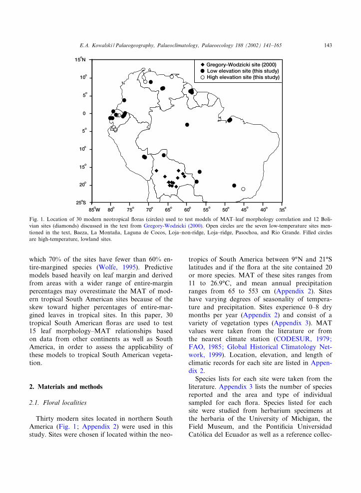
Thirty modern sites located in northern SouthAmerica (Fig. 1; Appendix 2) were used in thisstudy. Sites were chosen if located within the neo-

tropics of South America between 9‡N and 21‡Slatitudes and if the £ora at the site contained 20or more species. MAT of these sites ranges from11 to 26.9‡C, and mean annual precipitationranges from 65 to 553 cm (Appendix 2). Siteshave varying degrees of seasonality of tempera-ture and precipitation. Sites experience 0^8 drymonths per year (Appendix 2) and consist of avariety of vegetation types (Appendix 3). MATvalues were taken from the literature or fromthe nearest climate station (CODESUR, 1979;FAO, 1985; Global Historical Climatology Net-work, 1999). Location, elevation, and length ofclimatic records for each site are listed in Appen-dix 2.

Species lists for each site were taken from theliterature. Appendix 3 lists the number of speciesreported and the area and type of individualsampled for each £ora. Species listed for eachsite were studied from herbarium specimens atthe herbaria of the University of Michigan, theField Museum, and the Ponti¢cia UniversidadCato¤ lica del Ecuador as well as a reference collec-

Fig. 1. Location of 30 modern neotropical £oras (circles) used to test models of MAT^leaf morphology correlation and 12 Boli-vian sites (diamonds) discussed in the text from Gregory-Wodzicki (2000). Open circles are the seven low-temperature sites men-tioned in the text, Baeza, La Montan‹a, Laguna de Cocos, Loja^non-ridge, Loja^ridge, Pasochoa, and Rio Grande. Filled circlesare high-temperature, lowland sites.

PALAEO 2945 8-11-02

E.A. Kowalski / Palaeogeography, Palaeoclimatology, Palaeoecology 188 (2002) 141^165 143

tion of R.J. Burnham housed at the University ofMichigan. The location and elevation of eachspecimen as listed on the herbarium specimenwere recorded. Specimens collected at the inven-toried site were used to score 10% of all speciesscored. When no site-voucher was available,specimens were scored that had been collectedgeographically close to the inventoried site andfrom a similar elevation, so that the specimenscored came from a climatically similar area.Number of leaves per herbarium specimen variedfrom one to approximately 50.

Specimens were scored for the presence of 31leaf characters after Wolfe (1993) and Wolfe andSpicer (1999). In the original CLAMP databaseonly 29 characters were scored per site (Wolfe,1993). Later versions split the smallest and largestsize categories into two size classes each. None ofthe equations tested here rely on either of the sizeclasses that were split. The percentage of eachcharacter state among all species at each site islisted in Appendix 1. In total, 1823 specimenswere scored representing 1233 species. A total of208 species from the original £oral lists was notscored because the species were not present at theherbaria visited. The number of species scored foreach site is listed in Appendix 3. Species totals forall sites exceed the minimum 20 species recom-mended to predict MAT from leaf morphology(Wolfe, 1993; Povey et al., 1994). As the numberof species scored decreases, error increases be-cause each individual species contributes a larger

proportion of the total. Twenty species is sug-gested as the minimum number of species neces-sary to ensure that each species does not over-contribute to the total.

2.2. MAT models

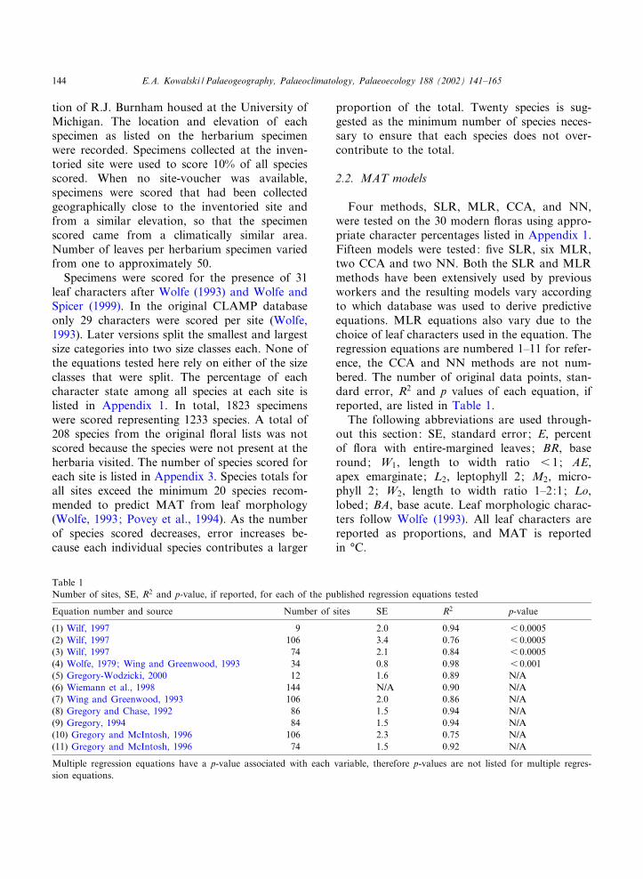
Four methods, SLR, MLR, CCA, and NN,were tested on the 30 modern £oras using appro-priate character percentages listed in Appendix 1.Fifteen models were tested: ¢ve SLR, six MLR,two CCA and two NN. Both the SLR and MLRmethods have been extensively used by previousworkers and the resulting models vary accordingto which database was used to derive predictiveequations. MLR equations also vary due to thechoice of leaf characters used in the equation. Theregression equations are numbered 1^11 for refer-ence, the CCA and NN methods are not num-bered. The number of original data points, stan-dard error, R2 and p values of each equation, ifreported, are listed in Table 1.

The following abbreviations are used through-out this section: SE, standard error; E, percentof £ora with entire-margined leaves; BR, baseround; W1, length to width ratio 6 1; AE,apex emarginate; L2, leptophyll 2; M2, micro-phyll 2; W2, length to width ratio 1^2:1; Lo,lobed; BA, base acute. Leaf morphologic charac-ters follow Wolfe (1993). All leaf characters arereported as proportions, and MAT is reportedin ‡C.

Table 1Number of sites, SE, R2 and p-value, if reported, for each of the published regression equations tested

Equation number and source Number of sites SE R2 p-value

(1) Wilf, 1997 9 2.0 0.94 6 0.0005(2) Wilf, 1997 106 3.4 0.76 6 0.0005(3) Wilf, 1997 74 2.1 0.84 6 0.0005(4) Wolfe, 1979; Wing and Greenwood, 1993 34 0.8 0.98 6 0.001(5) Gregory-Wodzicki, 2000 12 1.6 0.89 N/A(6) Wiemann et al., 1998 144 N/A 0.90 N/A(7) Wing and Greenwood, 1993 106 2.0 0.86 N/A(8) Gregory and Chase, 1992 86 1.5 0.94 N/A(9) Gregory, 1994 84 1.5 0.94 N/A(10) Gregory and McIntosh, 1996 106 2.3 0.75 N/A(11) Gregory and McIntosh, 1996 74 1.5 0.92 N/A

Multiple regression equations have a p-value associated with each variable, therefore p-values are not listed for multiple regres-sion equations.

PALAEO 2945 8-11-02


2.2.1. Simple linear regressionFive SLR equations that predict MAT from the

percentage of species with entire-margined leaveswere tested. The ¢rst three equations were origi-nally published in a study on the use of leaf mar-gin as a robust correlate of MAT (Wilf, 1997).Though not suggested for use as predictive equa-tions, these equations are published SLR equa-tions derived from the CLAMP database or sitesfrom both North and South America, so they weretested for their predictive value here. Wilf (1997)compiled a data set of nine sites from the WesternHemisphere ranging from Bolivia to Pennsylvania.His equation relating the percentage of specieswith entire-margined leaves and MAT is:

MAT ¼ 28:6E þ 2:24 ð1Þ

Two of the SLR equations are based on datafrom the 1993 CLAMP database (Wilf, 1997).The database used in this equation includes 106sites, primarily from North America:

MAT ¼ 29:1E30:266 ð2Þ

An abundance of cold sites in the CLAMP da-tabase increases the slope of the regression lineand lowers the value of the y-intercept. The resultis that MAT is often underestimated for warmsites when using a regression equation based onthe entire database. To eliminate the bias intro-duced by high numbers of cold sites, Wilf (1997)included a relationship in which the coldest 32sites, those with cold month mean temperaturesbelow 32‡C, were removed from the databaseused above prior to calculating the following re-gression:

MAT ¼ 24:4E þ 3:25 ð3Þ

The original regression that quanti¢ed the rela-tionship between leaf margin and temperature isbased on 34 sites from eastern Asia (Wolfe, 1979).Wing and Greenwood (1993) published the fol-lowing equation based on the graph of the origi-nal data from Wolfe (1979):

MAT ¼ 30:6E þ 1:14 ð4Þ

An equation from Gregory-Wodzicki (2000) isbased on data from 12 sites in Bolivia, along withtwo South American sites taken from Wilf (1997).This equation is unique in that the data comeonly from South America:

MAT ¼ 31:6E30:059 ð5Þ

2.2.2. Multiple regressionSix MLR equations were tested. The equations

use varying numbers of sites from di¡erent ver-sions of the CLAMP database to quantify therelationship between leaf morphology and MAT.Wiemann et al. (1998) derived an equation fromthe CLAMP 3B database:

MAT ¼ 0:207E30:058BR30:202W 1 þ 9:865

ð6Þ

Wing and Greenwood’s (1993) equation isbased on 106 CLAMP sites primarily from NorthAmerica. The values used to derive the equationwere ¢rst transformed by taking the arcsine indegrees of the square root of the proportion rep-resented by each percentage value before the re-gression analysis, to stabilize the variance ofbounded data (Sokal and Rohlf, 1995):

MAT ¼ 17:372E þ 2:896AE38:592W 1 þ 2:536

ð7Þ

Gregory (1994; Gregory and Chase, 1992;Gregory and McIntosh, 1996) has published sev-eral di¡erent regression equations based on theCLAMP data set. Four are included here. Dataused in the following four equations have under-gone arcsine transformation as described above.The following equation (Gregory and Chase,1992) is based on 86 CLAMP sites :

MAT ¼ 10:4E315:0L238:68W 1þ

4:74AE35:13M2 þ 16:1 ð8Þ

The following equation from Gregory (1994) isbased on 84 of the sites used in the previous equa-

PALAEO 2945 8-11-02


tion. The two coldest sites were removed to elim-inate any bias toward cold temperatures:

MAT ¼ 10:34E2 þ 5:48AE315:32W 21

315:29L235:79M2 þ 15:32 ð9Þ

Gregory and McIntosh (1996) proposed tworelationships, one is based on the 106-siteCLAMP database, and the other removes 32 siteswith cold month mean temperatures below 32‡C.All data were transformed by adding 0.005 to the

10

15

20

25

30

35

40A B

10

15

20

25

30

35

40C D

10

15

20

25

30

35

40E F

Pre

dic

ted

MAT

( C

)P

red

icte

d M

AT (

C)

Pre

dic

ted

MAT

( C

)

Observed MAT ( C)

Observed MAT ( C)

10

15

20

25

30

35

40

10 15 20 25 30 35 40

10 15 20 25 30 35 40

10

15

20

25

30

35

40

CCA -

G H

I

North America (6)

North America (9)North America (8)

North America (7)

CLAMP 3B - NN

CLAMP 3B CLAMP 3A - NN

North America (10) North America (11)

Pre

dic

ted

MAT

( C

)P

red

icte

d M

AT (

C)

o

o

o

o

o

o

o

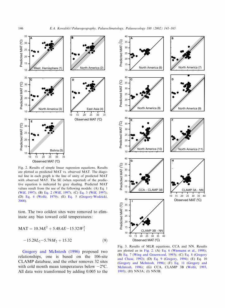
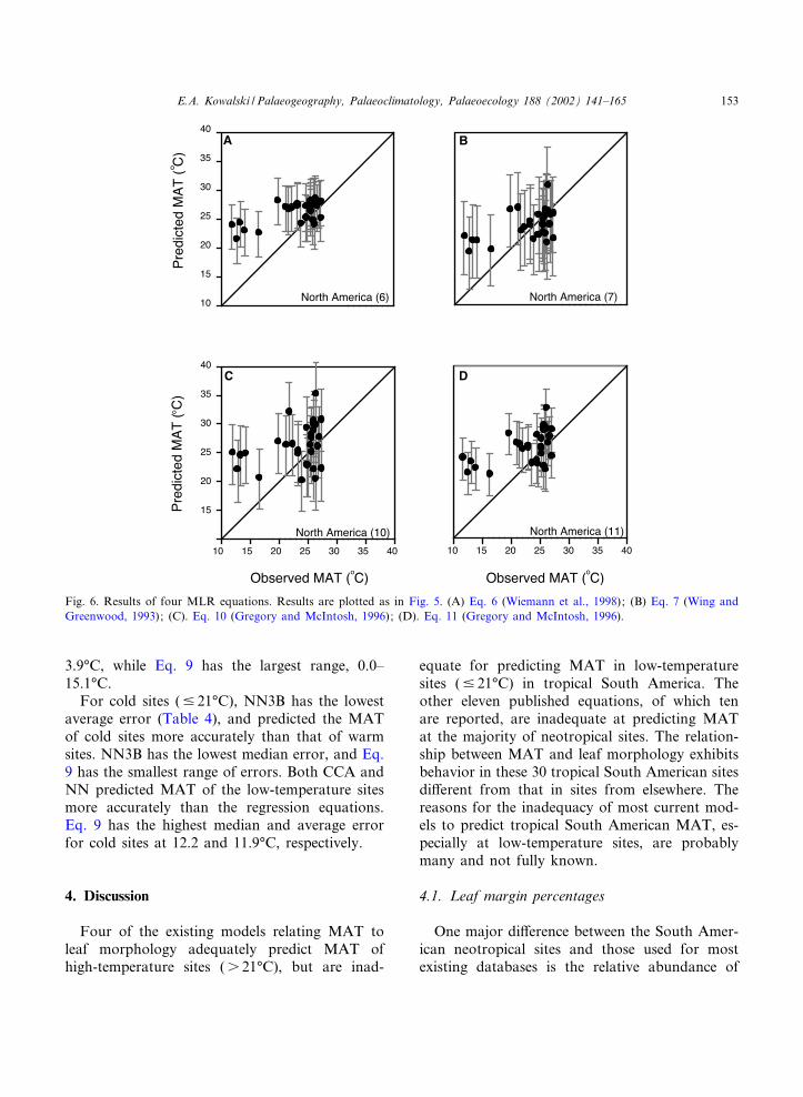
Fig. 3. Results of MLR equations, CCA and NN. Resultsare plotted as in Fig. 2. (A) Eq. 6 (Wiemann et al., 1998);(B) Eq. 7 (Wing and Greenwood, 1993); (C) Eq. 8 (Gregoryand Chase, 1992); (D) Eq. 9 (Gregory, 1994); (E) Eq. 10(Gregory and McIntosh, 1996); (F) Eq. 11 (Gregory andMcIntosh, 1996); (G) CCA, CLAMP 3B (Wolfe, 1993,1995); (H) NN3A; (I) NN3B.

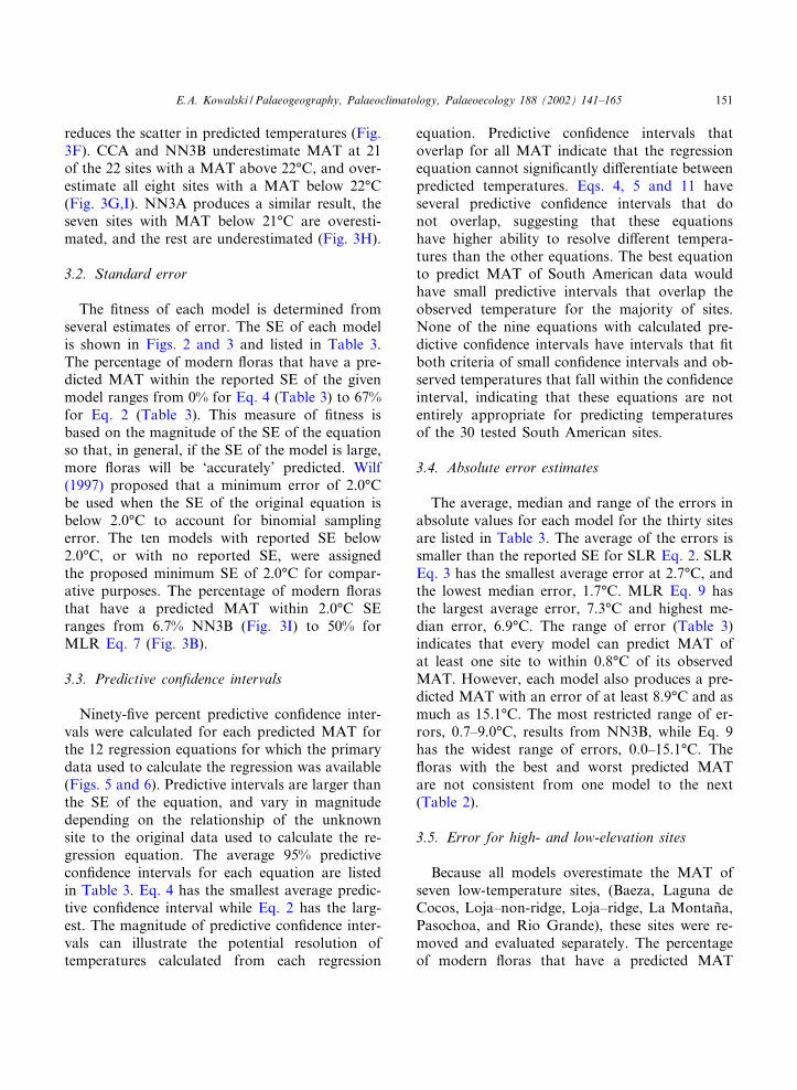
Fig. 2. Results of simple linear regression equations. Resultsare plotted as predicted MAT vs. observed MAT. The diago-nal line in each graph is the line of unity of predicted MATwith observed MAT. The SE (when reported) of the predic-tive equation is indicated by gray shading. Predicted MATvalues result from the use of the following models: (A) Eq. 1(Wilf, 1997); (B) Eq. 2 (Wilf, 1997); (C) Eq. 3 (Wilf, 1997);(D) Eq. 4 (Wolfe, 1979); (E) Eq. 5 (Gregory-Wodzicki,2000).

PALAEO 2945 8-11-02


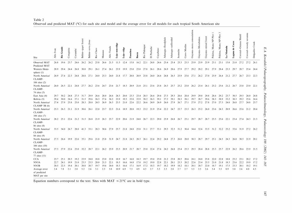
Table 2Observed and predicted MAT (‡C) for each site and model and the average error for all models for each tropical South American site

Site AltoIvan

RioGrande

Con

quista

Corum

ba¤

Bele¤m

--ig

apo¤forest

Bele¤m

--te

rra

firm

e

Rio

Claro

Man

aus

AltoYun

da

Loja--non-ridge

Loja--ridge

Pasochoa

Baeza

Rio

Palenqu

e

ElPechiche

Cuy

abeno

An‹ana

gu--floo

dplain

An‹ana

gu--un

floo

ded

Jaun

eche

Cerro

Mutiles

Guy

ana--m

oraconsociation

Guy

ana--M

orab

ukea

Guy

ana--m

ixed

forest

Pak

itsa,Man

uNPPlot1

Pak

itsa,Man

uNPPlot3

LaMontan‹a

LagunadeCocos

Corozal--Guian

aSh

ield

Corozal--woo

dysava

nna

Delga

dito

Creek

Observed MAT 26.8 19.6 23.7 24.6 26.2 26.2 25.8 26.6 21.5 11.5 12.4 13.8 16.2 22.1 24.8 24.6 25.4 25.4 25.3 25.5 25.9 25.9 25.9 23.1 23.1 13.0 21.0 27.2 27.2 26.1Predicted MATWestern Hemi-sphere (1)

28.9 29.4 24.4 26.8 30.8 29.1 26.1 27.4 26.1 23.9 19.9 23.0 23.0 27.8 26.1 28.6 26.9 28.6 27.9 27.7 29.2 28.2 29.1 27.9 28.4 23.3 29.7 28.7 25.4 24.4

North America/CLAMP-106 sites (2)

26.9 27.4 22.3 24.8 28.8 27.1 24.0 25.3 24.0 21.8 17.7 20.8 20.9 25.8 24.0 26.6 24.8 26.5 25.9 25.6 27.1 26.2 27.0 25.9 26.4 21.2 27.7 26.7 23.3 22.3


26.0 26.5 22.1 24.8 27.7 26.2 23.6 24.7 23.6 21.7 18.3 20.9 21.0 25.1 23.6 25.8 24.3 25.7 25.2 25.0 26.2 25.4 26.1 25.2 25.6 21.2 26.7 25.8 23.0 22.1

East Asia (4) 29.7 30.2 24.8 27.5 31.7 29.9 26.6 28.0 26.6 24.3 20.0 23.3 23.4 28.5 26.6 29.4 27.5 29.3 28.6 28.4 29.9 29.0 29.8 28.6 29.2 23.7 30.5 29.5 26.0 24.8Bolivia (5) 29.4 30.0 24.4 27.1 31.5 29.6 26.3 27.6 26.3 23.9 19.5 22.8 22.9 28.2 26.3 29.1 27.2 29.1 28.3 28.1 29.7 28.7 29.6 28.3 28.9 23.2 30.3 29.2 25.6 24.4North America/CLAMP 3B (6)

27.4 27.9 23.8 25.0 28.3 28.0 24.5 26.9 26.3 23.5 21.0 22.6 22.2 26.6 24.9 26.9 26.0 27.9 26.7 27.1 27.9 27.2 27.8 27.0 27.3 24.0 26.8 27.7 24.8 23.7


25.3 26.3 21.1 21.9 30.6 26.1 22.0 23.7 22.5 21.6 18.9 20.8 19.3 23.2 21.9 25.4 22.2 24.7 23.7 23.5 26.3 25.2 26.0 23.6 24.3 20.9 26.6 25.6 21.2 20.4


28.2 25.1 22.6 21.2 31.5 26.8 21.9 26.3 25.7 22.9 20.6 21.9 24.0 26.7 22.3 29.0 25.9 26.8 26.7 25.1 29.7 28.7 28.7 25.5 25.6 22.1 23.4 27.4 24.3 21.3


33.5 34.0 26.7 28.0 41.3 33.1 28.3 30.6 27.9 25.7 21.8 24.8 25.8 31.1 27.7 33.1 29.5 32.3 31.2 30.4 34.4 32.6 33.5 31.2 32.2 25.2 33.6 31.9 27.2 26.2


27.5 26.6 19.9 22.6 35.1 29.6 21.8 25.8 31.9 24.7 21.8 24.5 20.3 26.1 22.4 29.2 24.8 27.3 26.0 28.0 30.3 28.7 29.7 25.1 24.5 24.3 26.0 30.5 21.9 20.1


27.3 27.9 22.6 23.0 32.2 28.7 22.1 26.2 25.9 23.5 20.9 21.7 20.7 25.0 22.4 27.6 24.2 26.8 25.4 25.3 29.3 28.4 28.8 25.3 25.7 22.9 26.2 28.6 23.9 21.5

CCA 23.7 25.1 20.3 19.2 23.9 24.0 18.8 23.0 22.8 18.9 16.7 16.8 18.3 19.7 19.4 25.0 21.2 23.8 20.5 20.6 24.1 24.0 25.8 22.0 22.8 18.8 23.2 23.1 20.2 17.2NN3A 22.7 24.1 19.9 21.0 23.5 23.5 20.0 21.5 22.1 18.5 16.6 16.8 17.8 19.2 19.0 22.8 22.1 20.1 25.3 20.2 22.6 23.4 25.5 21.0 21.8 18.3 23.6 22.2 19.9 17.2NN3B 20.5 22.5 19.4 20.1 20.8 20.7 19.7 19.6 20.0 18.3 16.6 17.1 16.9 17.2 18.3 19.7 18.2 19.9 18.2 18.1 20.1 20.7 22.0 18.7 19.1 17.5 23.3 20.1 18.2 19.1Average errorof predictedMAT per site

2.4 7.8 2.1 2.8 5.2 2.6 3.1 2.3 3.8 10.9 6.9 7.5 4.9 4.3 2.7 3.3 2.3 2.8 2.7 2.7 3.3 2.5 2.6 3.4 3.5 8.9 5.8 2.6 4.0 4.5

Equation numbers correspond to the text. Sites with MAT 9 21‡C are in bold type.

PALAEO

29458-11-02

E.A

.Kow

alski/Palaeogeography,

Palaeoclim

atology,Palaeoecology

188(2002)

141^165147

raw percentage value, followed by arcsine trans-formation:

MAT ¼ 23:258E316:099W 1312:211L2þ

11:484W 2 þ 10:282Lo37:022BA311:262 ð10Þ

MAT ¼ 16:656E39:2L235:594W 1þ

5:137BA þ 4:879AE þ 1:768 ð11Þ

2.2.3. Multivariate statistical techniquesCCA on the CLAMP database was carried out

for this study using CANOCO Version 3.12 (terBraak, 1991), an ordination program used here toquantify the association between climatic varia-bles and leaf morphologic characters. The axisscores resulting from the ordination are convertedto absolute temperature values through multipleregression equations. Both CLAMP 3A, a 173-site

CLAMP database, and CLAMP 3B, a 144-siteCLAMP database that excludes 29 alpine andscrub outliers (Wolfe, 1995; Wolfe and Spicer,1999), were analyzed with CCA. Only the resultsfrom the CLAMP 3B analysis are reported. Boththe CLAMP database and the regression equa-tions are available online from Jack A. Wolfe(University of Arizona, Tucson, AZ).

The ¢nal method tested is CCA, followed by aNN resemblance function. Canoco Version 3.12was again used for the analysis. The ¢rst threeaxis scores resulting from the ordination wereused to determine the twenty sites in the CLAMPdatabase which are closest, using Euclidean dis-tance, to the unknown site (Stranks and England,1997). The MAT of the twenty nearest neighborsare then used as calibration data to determine theMAT of the test site, by calculating a regressionequation from the axis scores. Both the 173-siteCLAMP 3A and the 144-site CLAMP 3B data-bases were used with this method. The results of

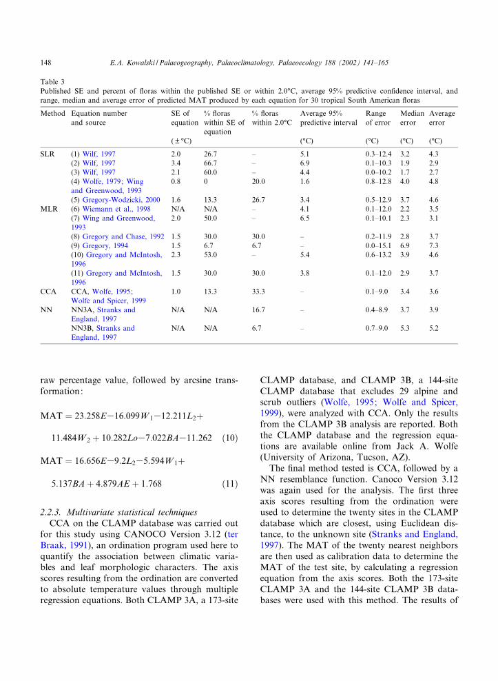
Table 3Published SE and percent of £oras within the published SE or within 2.0‡C, average 95% predictive con¢dence interval, andrange, median and average error of predicted MAT produced by each equation for 30 tropical South American £oras

Method Equation numberand source

SE ofequation

% £oraswithin SE ofequation

% £oraswithin 2.0‡C

Average 95%predictive interval

Rangeof error

Medianerror

Averageerror

( U ‡C) (‡C) (‡C) (‡C) (‡C)

SLR (1) Wilf, 1997 2.0 26.7 ^ 5.1 0.3^12.4 3.2 4.3(2) Wilf, 1997 3.4 66.7 ^ 6.9 0.1^10.3 1.9 2.9(3) Wilf, 1997 2.1 60.0 ^ 4.4 0.0^10.2 1.7 2.7(4) Wolfe, 1979; Wingand Greenwood, 1993

0.8 0 20.0 1.6 0.8^12.8 4.0 4.8

(5) Gregory-Wodzicki, 2000 1.6 13.3 26.7 3.4 0.5^12.9 3.7 4.6MLR (6) Wiemann et al., 1998 N/A N/A ^ 4.1 0.1^12.0 2.2 3.5

(7) Wing and Greenwood,1993

2.0 50.0 ^ 6.5 0.1^10.1 2.3 3.1

(8) Gregory and Chase, 1992 1.5 30.0 30.0 ^ 0.2^11.9 2.8 3.7(9) Gregory, 1994 1.5 6.7 6.7 ^ 0.0^15.1 6.9 7.3(10) Gregory and McIntosh,1996

2.3 53.0 ^ 5.4 0.6^13.2 3.9 4.6

(11) Gregory and McIntosh,1996

1.5 30.0 30.0 3.8 0.1^12.0 2.9 3.7

CCA CCA, Wolfe, 1995;Wolfe and Spicer, 1999

1.0 13.3 33.3 ^ 0.1^9.0 3.4 3.6

NN NN3A, Stranks andEngland, 1997

N/A N/A 16.7 ^ 0.4^8.9 3.7 3.9

NN3B, Stranks andEngland, 1997

N/A N/A 6.7 ^ 0.7^9.0 5.3 5.2

PALAEO 2945 8-11-02


each analysis are referred to as NN3A andNN3B, depending on whether CLAMP 3A or3B was used.

2.2.4. Error evaluationTemperatures were calculated for each site us-

ing the 15 models detailed above. Predicted MATwas compared to observed temperature for eachsite. Absolute average, median, and range of errorwere calculated for each equation. In addition, thepercentage of sites that are estimated within theSE of the equation and the average 95% predicted

con¢dence interval were calculated for each equa-tion.

3. Results

3.1. General results

Each of the tested models gave di¡erent results(Figs. 2 and 3; Tables 2^4), but some trends doemerge. All equations overestimate the MAT ofthe same seven modern sites with an observed

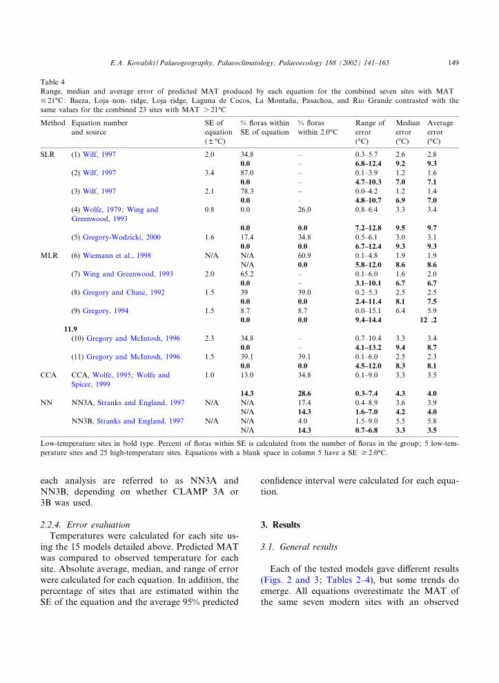
Table 4Range, median and average error of predicted MAT produced by each equation for the combined seven sites with MAT9 21‡C: Baeza, Loja^non- ridge, Loja^ridge, Laguna de Cocos, La Montan‹a, Pasachoa, and Rio Grande contrasted with thesame values for the combined 23 sites with MAT s 21‡C

Method Equation numberand source

SE ofequation

% £oras withinSE of equation

% £oraswithin 2.0‡C

Range oferror

Medianerror

Averageerror

( U ‡C) (‡C) (‡C) (‡C)

SLR (1) Wilf, 1997 2.0 34.8 ^ 0.3^5.7 2.6 2.80.0 ^ 6.8^12.4 9.2 9.3

(2) Wilf, 1997 3.4 87.0 ^ 0.1^3.9 1.2 1.60.0 ^ 4.7^10.3 7.0 7.1

(3) Wilf, 1997 2.1 78.3 ^ 0.0^4.2 1.2 1.40.0 ^ 4.8^10.7 6.9 7.0

(4) Wolfe, 1979; Wing andGreenwood, 1993

0.8 0.0 26.0 0.8^6.4 3.3 3.4

0.0 0.0 7.2^12.8 9.5 9.7(5) Gregory-Wodzicki, 2000 1.6 17.4 34.8 0.5^6.1 3.0 3.1

0.0 0.0 6.7^12.4 9.3 9.3MLR (6) Wiemann et al., 1998 N/A N/A 60.9 0.1^4.8 1.9 1.9

N/A 0.0 5.8^12.0 8.6 8.6(7) Wing and Greenwood, 1993 2.0 65.2 ^ 0.1^6.0 1.6 2.0

0.0 ^ 3.1^10.1 6.7 6.7(8) Gregory and Chase, 1992 1.5 39 39.0 0.2^5.3 2.5 2.5

0.0 0.0 2.4^11.4 8.1 7.5(9) Gregory, 1994 1.5 8.7 8.7 0.0^15.1 6.4 5.9

0.0 0.0 9.4^14.4 12 .211.9(10) Gregory and McIntosh, 1996 2.3 34.8 ^ 0.7^10.4 3.3 3.4

0.0 ^ 4.1^13.2 9.4 8.7(11) Gregory and McIntosh, 1996 1.5 39.1 39.1 0.1^6.0 2.5 2.3

0.0 0.0 4.5^12.0 8.3 8.1CCA CCA, Wolfe, 1995; Wolfe and

Spicer, 19991.0 13.0 34.8 0.1^9.0 3.3 3.5

14.3 28.6 0.3^7.4 4.3 4.0NN NN3A, Stranks and England, 1997 N/A N/A 17.4 0.4^8.9 3.6 3.9

N/A 14.3 1.6^7.0 4.2 4.0NN3B, Stranks and England, 1997 N/A N/A 4.0 1.5^9.0 5.5 5.8

N/A 14.3 0.7^6.8 3.3 3.5

Low-temperature sites in bold type. Percent of £oras within SE is calculated from the number of £oras in the group; 5 low-tem-perature sites and 25 high-temperature sites. Equations with a blank space in column 5 have a SE v 2.0‡C.

PALAEO 2945 8-11-02


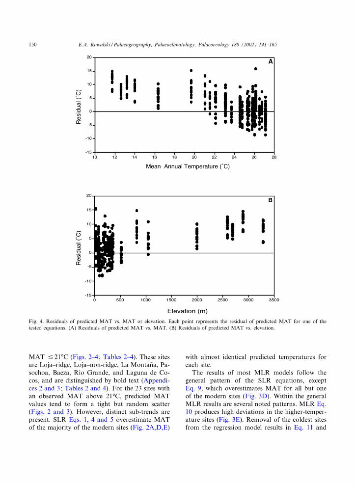
MAT 9 21‡C (Figs. 2^4; Tables 2^4). These sitesare Loja^ridge, Loja^non-ridge, La Montan‹a, Pa-sochoa, Baeza, Rio Grande, and Laguna de Co-cos, and are distinguished by bold text (Appendi-ces 2 and 3; Tables 2 and 4). For the 23 sites withan observed MAT above 21‡C, predicted MATvalues tend to form a tight but random scatter(Figs. 2 and 3). However, distinct sub-trends arepresent. SLR Eqs. 1, 4 and 5 overestimate MATof the majority of the modern sites (Fig. 2A,D,E)

with almost identical predicted temperatures foreach site.

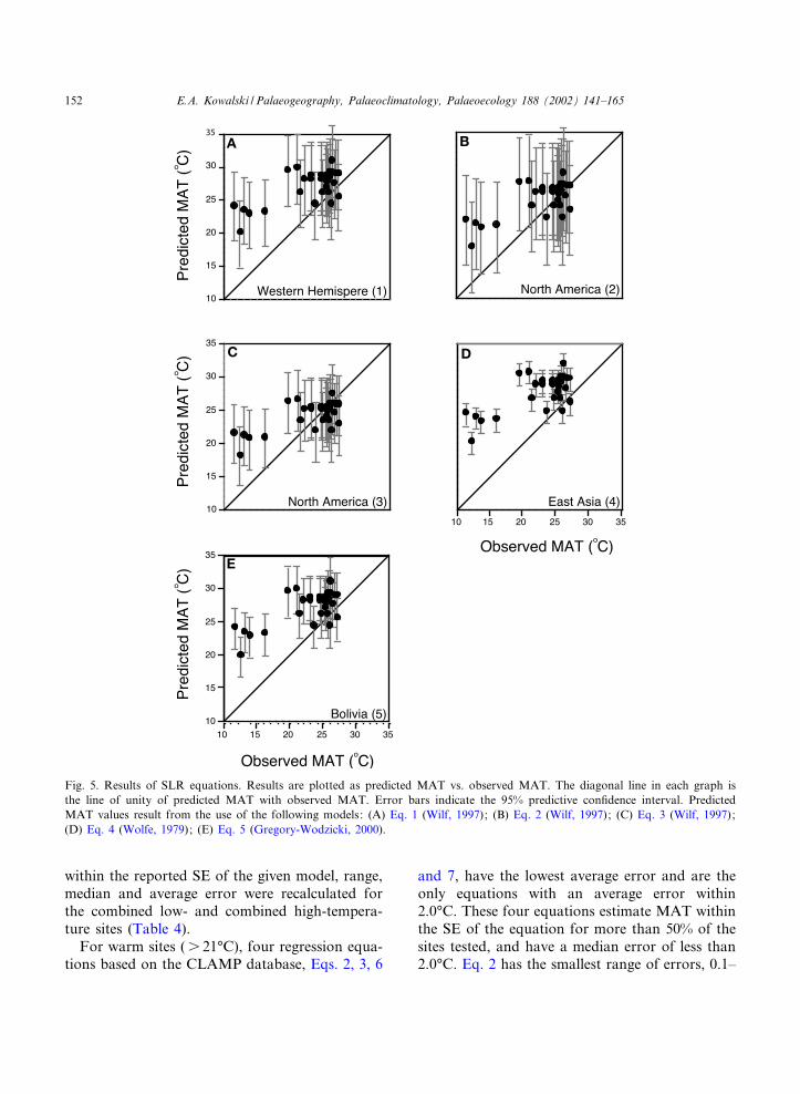
The results of most MLR models follow thegeneral pattern of the SLR equations, exceptEq. 9, which overestimates MAT for all but oneof the modern sites (Fig. 3D). Within the generalMLR results are several noted patterns. MLR Eq.10 produces high deviations in the higher-temper-ature sites (Fig. 3E). Removal of the coldest sitesfrom the regression model results in Eq. 11 and

Fig. 4. Residuals of predicted MAT vs. MAT or elevation. Each point represents the residual of predicted MAT for one of thetested equations. (A) Residuals of predicted MAT vs. MAT. (B) Residuals of predicted MAT vs. elevation.

PALAEO 2945 8-11-02


reduces the scatter in predicted temperatures (Fig.3F). CCA and NN3B underestimate MAT at 21of the 22 sites with a MAT above 22‡C, and over-estimate all eight sites with a MAT below 22‡C(Fig. 3G,I). NN3A produces a similar result, theseven sites with MAT below 21‡C are overesti-mated, and the rest are underestimated (Fig. 3H).

3.2. Standard error

The ¢tness of each model is determined fromseveral estimates of error. The SE of each modelis shown in Figs. 2 and 3 and listed in Table 3.The percentage of modern £oras that have a pre-dicted MAT within the reported SE of the givenmodel ranges from 0% for Eq. 4 (Table 3) to 67%for Eq. 2 (Table 3). This measure of ¢tness isbased on the magnitude of the SE of the equationso that, in general, if the SE of the model is large,more £oras will be ‘accurately’ predicted. Wilf(1997) proposed that a minimum error of 2.0‡Cbe used when the SE of the original equation isbelow 2.0‡C to account for binomial samplingerror. The ten models with reported SE below2.0‡C, or with no reported SE, were assignedthe proposed minimum SE of 2.0‡C for compar-ative purposes. The percentage of modern £orasthat have a predicted MAT within 2.0‡C SEranges from 6.7% NN3B (Fig. 3I) to 50% forMLR Eq. 7 (Fig. 3B).

3.3. Predictive con¢dence intervals

Ninety-¢ve percent predictive con¢dence inter-vals were calculated for each predicted MAT forthe 12 regression equations for which the primarydata used to calculate the regression was available(Figs. 5 and 6). Predictive intervals are larger thanthe SE of the equation, and vary in magnitudedepending on the relationship of the unknownsite to the original data used to calculate the re-gression equation. The average 95% predictivecon¢dence intervals for each equation are listedin Table 3. Eq. 4 has the smallest average predic-tive con¢dence interval while Eq. 2 has the larg-est. The magnitude of predictive con¢dence inter-vals can illustrate the potential resolution oftemperatures calculated from each regression

equation. Predictive con¢dence intervals thatoverlap for all MAT indicate that the regressionequation cannot signi¢cantly di¡erentiate betweenpredicted temperatures. Eqs. 4, 5 and 11 haveseveral predictive con¢dence intervals that donot overlap, suggesting that these equationshave higher ability to resolve di¡erent tempera-tures than the other equations. The best equationto predict MAT of South American data wouldhave small predictive intervals that overlap theobserved temperature for the majority of sites.None of the nine equations with calculated pre-dictive con¢dence intervals have intervals that ¢tboth criteria of small con¢dence intervals and ob-served temperatures that fall within the con¢denceinterval, indicating that these equations are notentirely appropriate for predicting temperaturesof the 30 tested South American sites.

3.4. Absolute error estimates

The average, median and range of the errors inabsolute values for each model for the thirty sitesare listed in Table 3. The average of the errors issmaller than the reported SE for SLR Eq. 2. SLREq. 3 has the smallest average error at 2.7‡C, andthe lowest median error, 1.7‡C. MLR Eq. 9 hasthe largest average error, 7.3‡C and highest me-dian error, 6.9‡C. The range of error (Table 3)indicates that every model can predict MAT ofat least one site to within 0.8‡C of its observedMAT. However, each model also produces a pre-dicted MAT with an error of at least 8.9‡C and asmuch as 15.1‡C. The most restricted range of er-rors, 0.7^9.0‡C, results from NN3B, while Eq. 9has the widest range of errors, 0.0^15.1‡C. The£oras with the best and worst predicted MATare not consistent from one model to the next(Table 2).

3.5. Error for high- and low-elevation sites

Because all models overestimate the MAT ofseven low-temperature sites, (Baeza, Laguna deCocos, Loja^non-ridge, Loja^ridge, La Montan‹a,Pasochoa, and Rio Grande), these sites were re-moved and evaluated separately. The percentageof modern £oras that have a predicted MAT

PALAEO 2945 8-11-02


within the reported SE of the given model, range,median and average error were recalculated forthe combined low- and combined high-tempera-ture sites (Table 4).

For warm sites (s 21‡C), four regression equa-tions based on the CLAMP database, Eqs. 2, 3, 6

and 7, have the lowest average error and are theonly equations with an average error within2.0‡C. These four equations estimate MAT withinthe SE of the equation for more than 50% of thesites tested, and have a median error of less than2.0‡C. Eq. 2 has the smallest range of errors, 0.1^

Fig. 5. Results of SLR equations. Results are plotted as predicted MAT vs. observed MAT. The diagonal line in each graph isthe line of unity of predicted MAT with observed MAT. Error bars indicate the 95% predictive con¢dence interval. PredictedMAT values result from the use of the following models: (A) Eq. 1 (Wilf, 1997); (B) Eq. 2 (Wilf, 1997); (C) Eq. 3 (Wilf, 1997);(D) Eq. 4 (Wolfe, 1979); (E) Eq. 5 (Gregory-Wodzicki, 2000).

PALAEO 2945 8-11-02


3.9‡C, while Eq. 9 has the largest range, 0.0^15.1‡C.

For cold sites (9 21‡C), NN3B has the lowestaverage error (Table 4), and predicted the MATof cold sites more accurately than that of warmsites. NN3B has the lowest median error, and Eq.9 has the smallest range of errors. Both CCA andNN predicted MAT of the low-temperature sitesmore accurately than the regression equations.Eq. 9 has the highest median and average errorfor cold sites at 12.2 and 11.9‡C, respectively.

4. Discussion

Four of the existing models relating MAT toleaf morphology adequately predict MAT ofhigh-temperature sites (s 21‡C), but are inad-

equate for predicting MAT in low-temperaturesites (9 21‡C) in tropical South America. Theother eleven published equations, of which tenare reported, are inadequate at predicting MATat the majority of neotropical sites. The relation-ship between MAT and leaf morphology exhibitsbehavior in these 30 tropical South American sitesdi¡erent from that in sites from elsewhere. Thereasons for the inadequacy of most current mod-els to predict tropical South American MAT, es-pecially at low-temperature sites, are probablymany and not fully known.

4.1. Leaf margin percentages

One major di¡erence between the South Amer-ican neotropical sites and those used for mostexisting databases is the relative abundance of

Fig. 6. Results of four MLR equations. Results are plotted as in Fig. 5. (A) Eq. 6 (Wiemann et al., 1998); (B) Eq. 7 (Wing andGreenwood, 1993); (C). Eq. 10 (Gregory and McIntosh, 1996); (D). Eq. 11 (Gregory and McIntosh, 1996).

PALAEO 2945 8-11-02


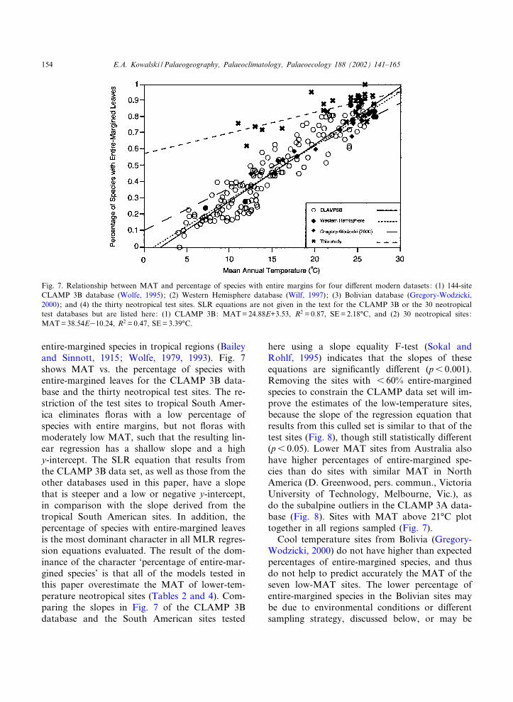
entire-margined species in tropical regions (Baileyand Sinnott, 1915; Wolfe, 1979, 1993). Fig. 7shows MAT vs. the percentage of species withentire-margined leaves for the CLAMP 3B data-base and the thirty neotropical test sites. The re-striction of the test sites to tropical South Amer-ica eliminates £oras with a low percentage ofspecies with entire margins, but not £oras withmoderately low MAT, such that the resulting lin-ear regression has a shallow slope and a highy-intercept. The SLR equation that results fromthe CLAMP 3B data set, as well as those from theother databases used in this paper, have a slopethat is steeper and a low or negative y-intercept,in comparison with the slope derived from thetropical South American sites. In addition, thepercentage of species with entire-margined leavesis the most dominant character in all MLR regres-sion equations evaluated. The result of the dom-inance of the character ‘percentage of entire-mar-gined species’ is that all of the models tested inthis paper overestimate the MAT of lower-tem-perature neotropical sites (Tables 2 and 4). Com-paring the slopes in Fig. 7 of the CLAMP 3Bdatabase and the South American sites tested

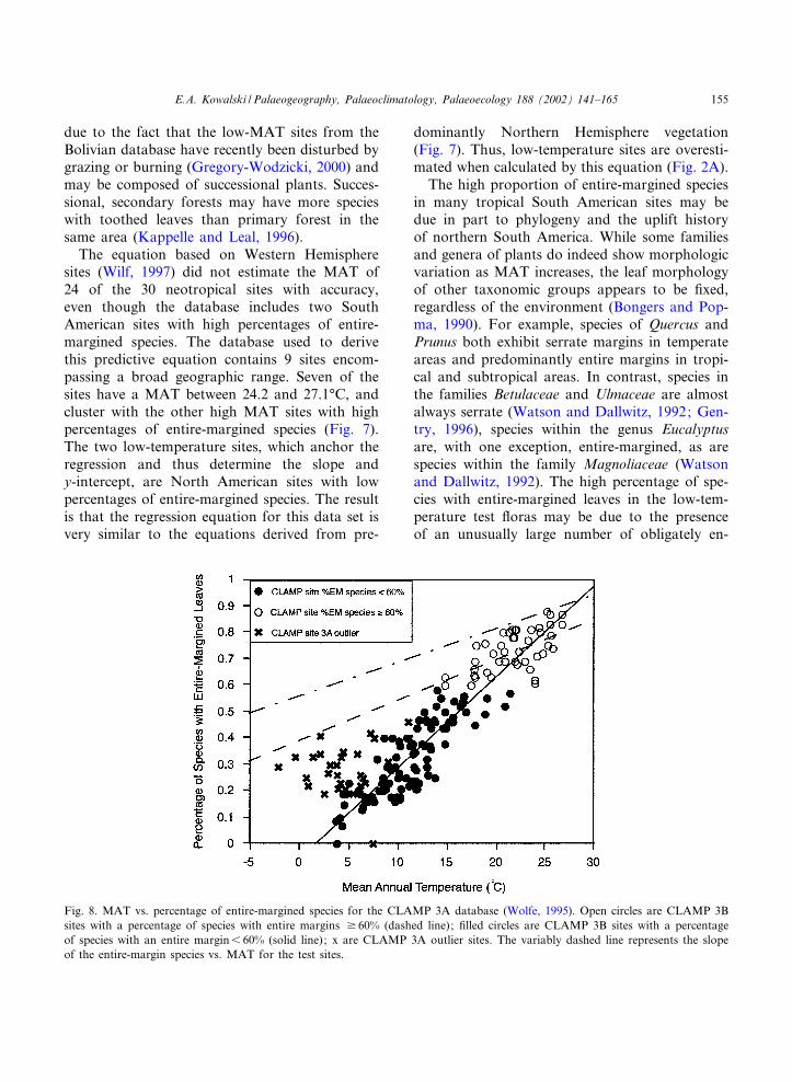
here using a slope equality F-test (Sokal andRohlf, 1995) indicates that the slopes of theseequations are signi¢cantly di¡erent (p6 0.001).Removing the sites with 6 60% entire-marginedspecies to constrain the CLAMP data set will im-prove the estimates of the low-temperature sites,because the slope of the regression equation thatresults from this culled set is similar to that of thetest sites (Fig. 8), though still statistically di¡erent(p6 0.05). Lower MAT sites from Australia alsohave higher percentages of entire-margined spe-cies than do sites with similar MAT in NorthAmerica (D. Greenwood, pers. commun., VictoriaUniversity of Technology, Melbourne, Vic.), asdo the subalpine outliers in the CLAMP 3A data-base (Fig. 8). Sites with MAT above 21‡C plottogether in all regions sampled (Fig. 7).

Cool temperature sites from Bolivia (Gregory-Wodzicki, 2000) do not have higher than expectedpercentages of entire-margined species, and thusdo not help to predict accurately the MAT of theseven low-MAT sites. The lower percentage ofentire-margined species in the Bolivian sites maybe due to environmental conditions or di¡erentsampling strategy, discussed below, or may be

Fig. 7. Relationship between MAT and percentage of species with entire margins for four di¡erent modern datasets: (1) 144-siteCLAMP 3B database (Wolfe, 1995); (2) Western Hemisphere database (Wilf, 1997); (3) Bolivian database (Gregory-Wodzicki,2000); and (4) the thirty neotropical test sites. SLR equations are not given in the text for the CLAMP 3B or the 30 neotropicaltest databases but are listed here: (1) CLAMP 3B: MAT=24.88E+3.53, R2 = 0.87, SE=2.18‡C, and (2) 30 neotropical sites:MAT=38.54E310.24, R2 = 0.47, SE=3.39‡C.

PALAEO 2945 8-11-02


due to the fact that the low-MAT sites from theBolivian database have recently been disturbed bygrazing or burning (Gregory-Wodzicki, 2000) andmay be composed of successional plants. Succes-sional, secondary forests may have more specieswith toothed leaves than primary forest in thesame area (Kappelle and Leal, 1996).

The equation based on Western Hemispheresites (Wilf, 1997) did not estimate the MAT of24 of the 30 neotropical sites with accuracy,even though the database includes two SouthAmerican sites with high percentages of entire-margined species. The database used to derivethis predictive equation contains 9 sites encom-passing a broad geographic range. Seven of thesites have a MAT between 24.2 and 27.1‡C, andcluster with the other high MAT sites with highpercentages of entire-margined species (Fig. 7).The two low-temperature sites, which anchor theregression and thus determine the slope andy-intercept, are North American sites with lowpercentages of entire-margined species. The resultis that the regression equation for this data set isvery similar to the equations derived from pre-

dominantly Northern Hemisphere vegetation(Fig. 7). Thus, low-temperature sites are overesti-mated when calculated by this equation (Fig. 2A).

The high proportion of entire-margined speciesin many tropical South American sites may bedue in part to phylogeny and the uplift historyof northern South America. While some familiesand genera of plants do indeed show morphologicvariation as MAT increases, the leaf morphologyof other taxonomic groups appears to be ¢xed,regardless of the environment (Bongers and Pop-ma, 1990). For example, species of Quercus andPrunus both exhibit serrate margins in temperateareas and predominantly entire margins in tropi-cal and subtropical areas. In contrast, species inthe families Betulaceae and Ulmaceae are almostalways serrate (Watson and Dallwitz, 1992; Gen-try, 1996), species within the genus Eucalyptusare, with one exception, entire-margined, as arespecies within the family Magnoliaceae (Watsonand Dallwitz, 1992). The high percentage of spe-cies with entire-margined leaves in the low-tem-perature test £oras may be due to the presenceof an unusually large number of obligately en-

Fig. 8. MAT vs. percentage of entire-margined species for the CLAMP 3A database (Wolfe, 1995). Open circles are CLAMP 3Bsites with a percentage of species with entire margins v 60% (dashed line); ¢lled circles are CLAMP 3B sites with a percentageof species with an entire margin6 60% (solid line); x are CLAMP 3A outlier sites. The variably dashed line represents the slopeof the entire-margin species vs. MAT for the test sites.

PALAEO 2945 8-11-02


tire-margined lineages. Further investigation isneeded to ascertain if this is the case.

In addition, the uplift history of northern SouthAmerica in£uenced the migration and evolution-ary history of plants in the neotropics. Until thelate Oligocene (Graham, 1995; Wijninga, 1995), acontinuous lowland tropical environment existedin northern South America. During the past 25million years, the climate changed as the Andesbegan to uplift, but it did not approach modernconditions until the Pliocene, approximately 4 mil-lion years ago (Wijninga, 1995). In the nearlyhomogeneous climate, morphologic characterssuited to tropical conditions evolved, and thelack of high-elevation, low-temperature areas dis-couraged the migration of temperate plants. Withthe recent uplift of the Andes, migration of tem-perate elements such as Alnus and Juglans began(Burnham and Graham, 1999). Possibly, the shortperiod of time that has elapsed since the creationof high-elevation, low-temperature sites in theneotropics has not been long enough for a signi¢-cant proportion of the £ora to have migratedfrom temperate areas or to have evolved in re-sponse to lower MAT. Six of the seven low-tem-perature sites with higher then expected percen-tages of entire-margined leaves are located above800 m, indicating that uplift history may havein£uenced the plant species composition of thesesites.

The distinctive leaf physiognomy of some of thehigh-elevation sites may also be related to envi-ronmental conditions. Five of the low-tempera-ture sites are above 2000 m elevation and experi-ence over 140 cm of rainfall each year (Appendix2). These values are often associated with cloudforest, an environment usually characterized byhigh humidity and low temperatures. Leaves incloud forest tend to be small, thick, and entire-margined (Leigh, 1999). The reasons for this par-ticular leaf morphology are unknown, but explan-ations range from low soil nutrient levels to windprotection or low transpiration rates (Leigh,1999). The ¢ve highest-elevation sites tested herehave species that exhibit leaf morphologies similarto those of cloud-forest species, with large percen-tages of species with entire-margined leaves. Incontrast, the high-elevation sites from the Boliv-

ian database receive 6 100 cm of rain and havehigher percentages of toothed leaves (Gregory-Wodzicki, 2000). Large amounts of rainfall athigh elevations combined with low temperaturemay foster the growth of a disproportionate num-ber of species with entire-margined leaves. Thus,the plant species growing in the ¢ve high-eleva-tion, wet sites show a di¡erent relationship be-tween temperature and leaf-margin than plantspecies growing in other environments. The resultof this di¡erence in species composition may bethe overestimation of MAT by most equations athigh-elevation sites (Fig. 4B).

4.2. Rainfall

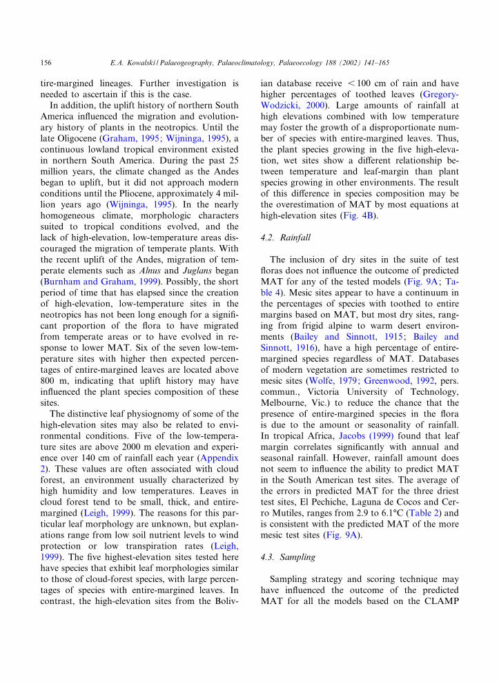
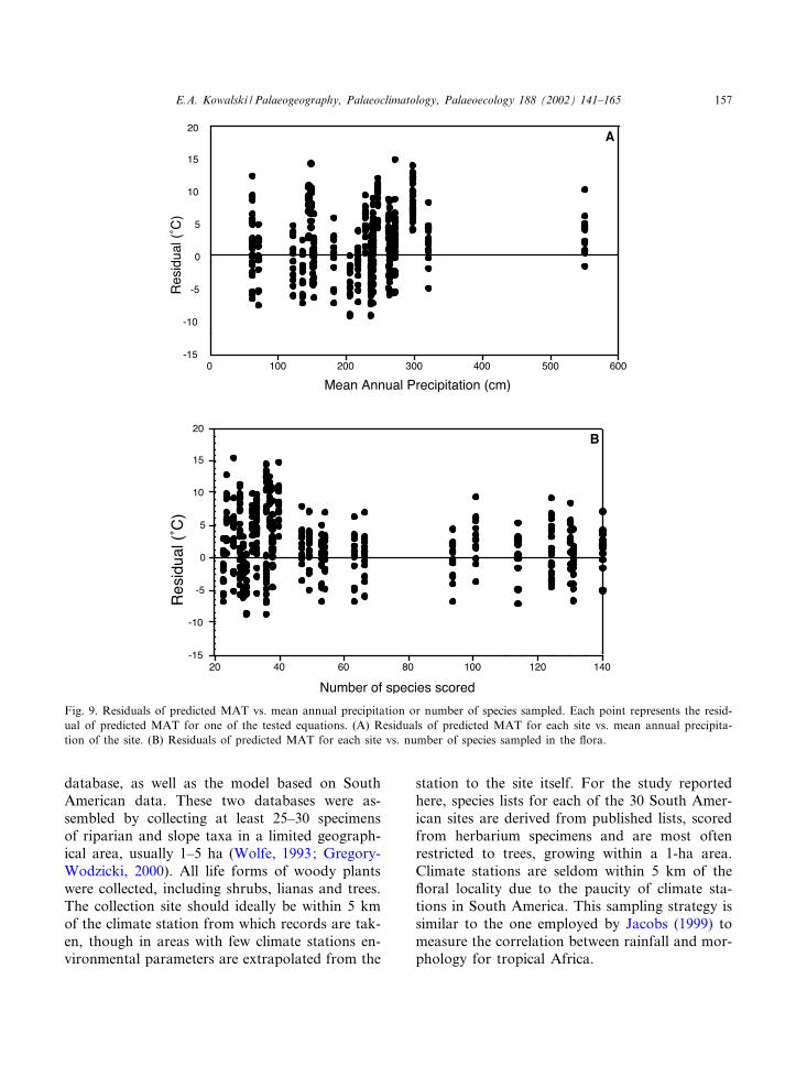
The inclusion of dry sites in the suite of test£oras does not in£uence the outcome of predictedMAT for any of the tested models (Fig. 9A; Ta-ble 4). Mesic sites appear to have a continuum inthe percentages of species with toothed to entiremargins based on MAT, but most dry sites, rang-ing from frigid alpine to warm desert environ-ments (Bailey and Sinnott, 1915; Bailey andSinnott, 1916), have a high percentage of entire-margined species regardless of MAT. Databasesof modern vegetation are sometimes restricted tomesic sites (Wolfe, 1979; Greenwood, 1992, pers.commun., Victoria University of Technology,Melbourne, Vic.) to reduce the chance that thepresence of entire-margined species in the £orais due to the amount or seasonality of rainfall.In tropical Africa, Jacobs (1999) found that leafmargin correlates signi¢cantly with annual andseasonal rainfall. However, rainfall amount doesnot seem to in£uence the ability to predict MATin the South American test sites. The average ofthe errors in predicted MAT for the three driesttest sites, El Pechiche, Laguna de Cocos and Cer-ro Mutiles, ranges from 2.9 to 6.1‡C (Table 2) andis consistent with the predicted MAT of the moremesic test sites (Fig. 9A).

4.3. Sampling

Sampling strategy and scoring technique mayhave in£uenced the outcome of the predictedMAT for all the models based on the CLAMP

PALAEO 2945 8-11-02


database, as well as the model based on SouthAmerican data. These two databases were as-sembled by collecting at least 25^30 specimensof riparian and slope taxa in a limited geograph-ical area, usually 1^5 ha (Wolfe, 1993; Gregory-Wodzicki, 2000). All life forms of woody plantswere collected, including shrubs, lianas and trees.The collection site should ideally be within 5 kmof the climate station from which records are tak-en, though in areas with few climate stations en-vironmental parameters are extrapolated from the

station to the site itself. For the study reportedhere, species lists for each of the 30 South Amer-ican sites are derived from published lists, scoredfrom herbarium specimens and are most oftenrestricted to trees, growing within a 1-ha area.Climate stations are seldom within 5 km of the£oral locality due to the paucity of climate sta-tions in South America. This sampling strategy issimilar to the one employed by Jacobs (1999) tomeasure the correlation between rainfall and mor-phology for tropical Africa.

Fig. 9. Residuals of predicted MAT vs. mean annual precipitation or number of species sampled. Each point represents the resid-ual of predicted MAT for one of the tested equations. (A) Residuals of predicted MAT for each site vs. mean annual precipita-tion of the site. (B) Residuals of predicted MAT for each site vs. number of species sampled in the £ora.

PALAEO 2945 8-11-02


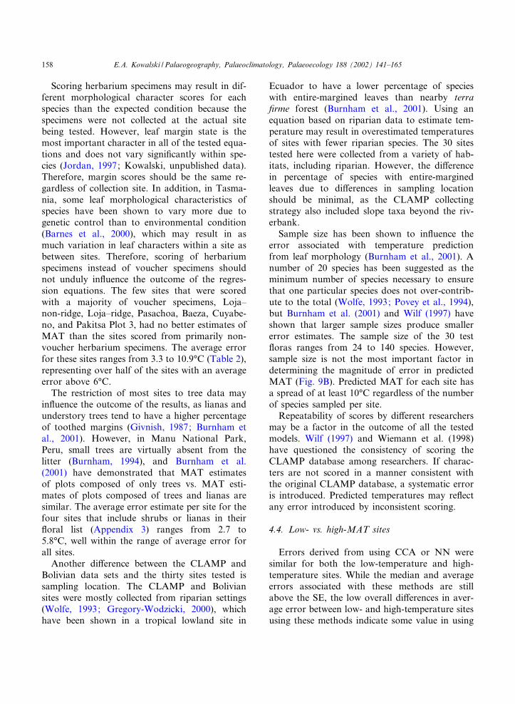
Scoring herbarium specimens may result in dif-ferent morphological character scores for eachspecies than the expected condition because thespecimens were not collected at the actual sitebeing tested. However, leaf margin state is themost important character in all of the tested equa-tions and does not vary signi¢cantly within spe-cies (Jordan, 1997; Kowalski, unpublished data).Therefore, margin scores should be the same re-gardless of collection site. In addition, in Tasma-nia, some leaf morphological characteristics ofspecies have been shown to vary more due togenetic control than to environmental condition(Barnes et al., 2000), which may result in asmuch variation in leaf characters within a site asbetween sites. Therefore, scoring of herbariumspecimens instead of voucher specimens shouldnot unduly in£uence the outcome of the regres-sion equations. The few sites that were scoredwith a majority of voucher specimens, Loja^non-ridge, Loja^ridge, Pasachoa, Baeza, Cuyabe-no, and Pakitsa Plot 3, had no better estimates ofMAT than the sites scored from primarily non-voucher herbarium specimens. The average errorfor these sites ranges from 3.3 to 10.9‡C (Table 2),representing over half of the sites with an averageerror above 6‡C.

The restriction of most sites to tree data mayin£uence the outcome of the results, as lianas andunderstory trees tend to have a higher percentageof toothed margins (Givnish, 1987; Burnham etal., 2001). However, in Manu National Park,Peru, small trees are virtually absent from thelitter (Burnham, 1994), and Burnham et al.(2001) have demonstrated that MAT estimatesof plots composed of only trees vs. MAT esti-mates of plots composed of trees and lianas aresimilar. The average error estimate per site for thefour sites that include shrubs or lianas in their£oral list (Appendix 3) ranges from 2.7 to5.8‡C, well within the range of average error forall sites.

Another di¡erence between the CLAMP andBolivian data sets and the thirty sites tested issampling location. The CLAMP and Boliviansites were mostly collected from riparian settings(Wolfe, 1993; Gregory-Wodzicki, 2000), whichhave been shown in a tropical lowland site in

Ecuador to have a lower percentage of specieswith entire-margined leaves than nearby terra¢rme forest (Burnham et al., 2001). Using anequation based on riparian data to estimate tem-perature may result in overestimated temperaturesof sites with fewer riparian species. The 30 sitestested here were collected from a variety of hab-itats, including riparian. However, the di¡erencein percentage of species with entire-marginedleaves due to di¡erences in sampling locationshould be minimal, as the CLAMP collectingstrategy also included slope taxa beyond the riv-erbank.

Sample size has been shown to in£uence theerror associated with temperature predictionfrom leaf morphology (Burnham et al., 2001). Anumber of 20 species has been suggested as theminimum number of species necessary to ensurethat one particular species does not over-contrib-ute to the total (Wolfe, 1993; Povey et al., 1994),but Burnham et al. (2001) and Wilf (1997) haveshown that larger sample sizes produce smallererror estimates. The sample size of the 30 test£oras ranges from 24 to 140 species. However,sample size is not the most important factor indetermining the magnitude of error in predictedMAT (Fig. 9B). Predicted MAT for each site hasa spread of at least 10‡C regardless of the numberof species sampled per site.

Repeatability of scores by di¡erent researchersmay be a factor in the outcome of all the testedmodels. Wilf (1997) and Wiemann et al. (1998)have questioned the consistency of scoring theCLAMP database among researchers. If charac-ters are not scored in a manner consistent withthe original CLAMP database, a systematic erroris introduced. Predicted temperatures may re£ectany error introduced by inconsistent scoring.

4.4. Low- vs. high-MAT sites

Errors derived from using CCA or NN weresimilar for both the low-temperature and high-temperature sites. While the median and averageerrors associated with these methods are stillabove the SE, the low overall di¡erences in aver-age error between low- and high-temperature sitesusing these methods indicate some value in using

PALAEO 2945 8-11-02


multivariate statistical techniques in tropical low-temperature environments. Every model testedhere overestimates MAT of the ¢ve low-temper-ature sites. However, for CCA and NN the pre-dicted site with the largest residual of estimatedMAT is one of the high-temperature sites (Table4). This suggests that although leaf margin state isthe single character most correlated with MAT,leaf morphologic characters other than marginare important in explaining the variation in pre-dicted MAT of tropical South America.

The seven low-temperature sites tested here canbe seen as outliers from the general relationshipbetween leaf-margin state and MAT. However,the multivariate models tested here using the full31 leaf morphologic characters from CLAMPfared as well predicting the seven low-temperaturesites as in predicting the high-temperature sites.The results presented here suggest these sevensites should not be treated as outliers, but as im-portant sites sampling the diversity of leaf mor-phologic assemblages in tropical South America,and should be incorporated into equations thatdetermine climate from leaf morphology.

5. Conclusions

I suggest that most current leaf morphology^MAT equations may not be appropriate for usein the South American tropics for low-MAT orhigh-elevation sites. It is important to test modelsof correlation between leaf morphology and cli-mate using data from modern analogous vegeta-tion before using that model to predict paleocli-mate from fossil vegetation. Using equationsgenerated from forests unrelated to those forwhich they are designed may result in poor esti-mates of paleo-MAT that are in error by as muchas 15.4‡C.

Predicting paleoclimate in tropical South Amer-ica can involve uncertainty of the elevation andprecipitation totals of a fossil site during its depo-sition, due to the continued uplift of the Andesand changing climatic patterns throughout theCenozoic. Because elevation and precipitation to-tals are not always known, equations that use leafmorphology to predict paleotemperature of Late

Cenozoic neotropical sites must be able to accu-rately predict MAT of sites over a wide range ofelevations and precipitation totals. Several of theequations tested here, Eqs. 2, 3, 6 and 7, accu-rately predict the majority of the high-tempera-ture sites and might be considered for use in pre-dicting MAT of fossil sites of known hightemperature or low elevation. However, none ofthe models tested here consistently predicts theMAT of low-temperature or high-elevation trop-ical South American sites, suggesting that theMAT of these sites would be best estimated bya correlation between MAT and leaf morphologyderived from the extensive data from tropicalSouth America, not from the Northern Hemi-sphere or Asia.

Acknowledgements

The author thanks N. Pitman and P. Nun‹ez forgenerously sharing their inventories for the twoPakitsa, Manu National Park, tree plots, J. Wolfefor access to the CLAMP database, R.J. Burn-ham for use of voucher specimens from Pakitsa,Manu National Park, and the herbaria of F,MICH and QCNE for access to herbarium speci-mens. The author also wishes to thank J. Bloch,B. Wilkinson, R. Burnham, D. Greenwood, P.Wilf, R. Madden, C. Badgley, W. Kuerschner,K. Gregory-Wodzicki, J. Wolfe, and an anony-mous reviewer for helpful discussion and com-ments on this manuscript.

PALAEO 2945 8-11-02


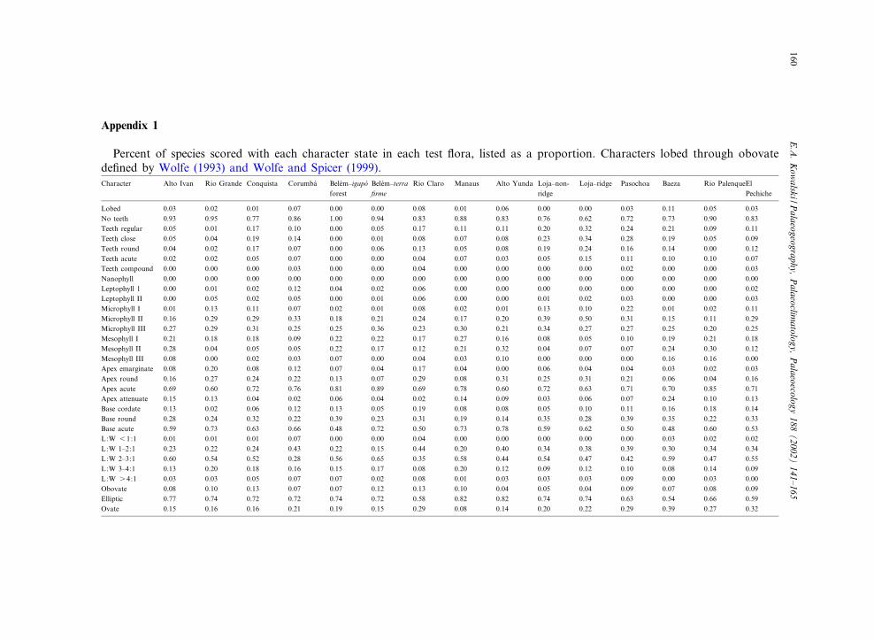
Appendix 1

Percent of species scored with each character state in each test £ora, listed as a proportion. Characters lobed through obovatede¢ned by Wolfe (1993) and Wolfe and Spicer (1999).Character Alto Ivan Rio Grande Conquista Corumba¤ Bele¤mîgapo¤

forestBele¤m^terra¢rme

Rio Claro Manaus Alto Yunda Loja^non-ridge

Loja^ridge Pasochoa Baeza Rio PalenqueElPechiche

Lobed 0.03 0.02 0.01 0.07 0.00 0.00 0.08 0.01 0.06 0.00 0.00 0.03 0.11 0.05 0.03No teeth 0.93 0.95 0.77 0.86 1.00 0.94 0.83 0.88 0.83 0.76 0.62 0.72 0.73 0.90 0.83Teeth regular 0.05 0.01 0.17 0.10 0.00 0.05 0.17 0.11 0.11 0.20 0.32 0.24 0.21 0.09 0.11Teeth close 0.05 0.04 0.19 0.14 0.00 0.01 0.08 0.07 0.08 0.23 0.34 0.28 0.19 0.05 0.09Teeth round 0.04 0.02 0.17 0.07 0.00 0.06 0.13 0.05 0.08 0.19 0.24 0.16 0.14 0.00 0.12Teeth acute 0.02 0.02 0.05 0.07 0.00 0.00 0.04 0.07 0.03 0.05 0.15 0.11 0.10 0.10 0.07Teeth compound 0.00 0.00 0.00 0.03 0.00 0.00 0.04 0.00 0.00 0.00 0.00 0.02 0.00 0.00 0.03Nanophyll 0.00 0.00 0.00 0.00 0.00 0.00 0.00 0.00 0.00 0.00 0.00 0.00 0.00 0.00 0.00Leptophyll 1 0.00 0.01 0.02 0.12 0.04 0.02 0.06 0.00 0.00 0.00 0.00 0.00 0.00 0.00 0.02Leptophyll II 0.00 0.05 0.02 0.05 0.00 0.01 0.06 0.00 0.00 0.01 0.02 0.03 0.00 0.00 0.03Microphyll I 0.01 0.13 0.11 0.07 0.02 0.01 0.08 0.02 0.01 0.13 0.10 0.22 0.01 0.02 0.11Microphyll II 0.16 0.29 0.29 0.33 0.18 0.21 0.24 0.17 0.20 0.39 0.50 0.31 0.15 0.11 0.29Microphyll III 0.27 0.29 0.31 0.25 0.25 0.36 0.23 0.30 0.21 0.34 0.27 0.27 0.25 0.20 0.25Mesophyll I 0.21 0.18 0.18 0.09 0.22 0.22 0.17 0.27 0.16 0.08 0.05 0.10 0.19 0.21 0.18Mesophyll II 0.28 0.04 0.05 0.05 0.22 0.17 0.12 0.21 0.32 0.04 0.07 0.07 0.24 0.30 0.12Mesophyll III 0.08 0.00 0.02 0.03 0.07 0.00 0.04 0.03 0.10 0.00 0.00 0.00 0.16 0.16 0.00Apex emarginate 0.08 0.20 0.08 0.12 0.07 0.04 0.17 0.04 0.00 0.06 0.04 0.04 0.03 0.02 0.03Apex round 0.16 0.27 0.24 0.22 0.13 0.07 0.29 0.08 0.31 0.25 0.31 0.21 0.06 0.04 0.16Apex acute 0.69 0.60 0.72 0.76 0.81 0.89 0.69 0.78 0.60 0.72 0.63 0.71 0.70 0.85 0.71Apex attenuate 0.15 0.13 0.04 0.02 0.06 0.04 0.02 0.14 0.09 0.03 0.06 0.07 0.24 0.10 0.13Base cordate 0.13 0.02 0.06 0.12 0.13 0.05 0.19 0.08 0.08 0.05 0.10 0.11 0.16 0.18 0.14Base round 0.28 0.24 0.32 0.22 0.39 0.23 0.31 0.19 0.14 0.35 0.28 0.39 0.35 0.22 0.33Base acute 0.59 0.73 0.63 0.66 0.48 0.72 0.50 0.73 0.78 0.59 0.62 0.50 0.48 0.60 0.53L:W 6 1:1 0.01 0.01 0.01 0.07 0.00 0.00 0.04 0.00 0.00 0.00 0.00 0.00 0.03 0.02 0.02L:W 1^2:1 0.23 0.22 0.24 0.43 0.22 0.15 0.44 0.20 0.40 0.34 0.38 0.39 0.30 0.34 0.34L:W 2^3:1 0.60 0.54 0.52 0.28 0.56 0.65 0.35 0.58 0.44 0.54 0.47 0.42 0.59 0.47 0.55L:W 3^4:1 0.13 0.20 0.18 0.16 0.15 0.17 0.08 0.20 0.12 0.09 0.12 0.10 0.08 0.14 0.09L:W s 4:1 0.03 0.03 0.05 0.07 0.07 0.02 0.08 0.01 0.03 0.03 0.03 0.09 0.00 0.03 0.00Obovate 0.08 0.10 0.13 0.07 0.07 0.12 0.13 0.10 0.04 0.05 0.04 0.09 0.07 0.08 0.09Elliptic 0.77 0.74 0.72 0.72 0.74 0.72 0.58 0.82 0.82 0.74 0.74 0.63 0.54 0.66 0.59Ovate 0.15 0.16 0.16 0.21 0.19 0.15 0.29 0.08 0.14 0.20 0.22 0.29 0.39 0.27 0.32

PALAEO

29458-11-02

E.A

.Kow


Palaeoclim


188(2002)

141^165160

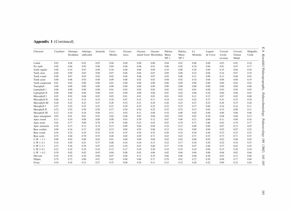
Appendix 1 (Continued).

Character Cuyabeno An‹anagu^£oodplain

An‹anaguûn£ooded

Jauneche CerroMutiles

Guyana^mora

Guyana^mixed forest

Guyana^Morabukea

Pakitsa,ManuNP 1

Pakitsa,ManuNP 3

LaMontan‹a

Lagunade Cocos

Corozal^woodysavanna

Corozal^GuianaShield

DelgaditoCreek

Lobed 0.03 0.04 0.01 0.02 0.04 0.00 0.00 0.00 0.04 0.03 0.00 0.00 0.03 0.02 0.10No teeth 0.92 0.86 0.92 0.90 0.89 0.94 0.94 0.91 0.90 0.92 0.74 0.96 0.81 0.93 0.77Teeth regular 0.08 0.14 0.07 0.09 0.10 0.06 0.06 0.09 0.10 0.08 0.24 0.04 0.19 0.06 0.20Teeth close 0.04 0.09 0.05 0.08 0.07 0.06 0.04 0.07 0.09 0.08 0.22 0.04 0.16 0.07 0.19Teeth round 0.08 0.07 0.05 0.02 0.02 0.06 0.04 0.07 0.05 0.06 0.11 0.00 0.11 0.04 0.03Teeth acute 0.00 0.06 0.03 0.08 0.09 0.00 0.02 0.02 0.04 0.02 0.14 0.04 0.08 0.04 0.19Teeth compound 0.01 0.02 0.00 0.00 0.01 0.00 0.00 0.00 0.00 0.00 0.00 0.00 0.00 0.02 0.03Nanophyll 0.00 0.00 0.00 0.00 0.00 0.00 0.00 0.00 0.00 0.00 0.00 0.00 0.00 0.00 0.00Leptophyll 1 0.00 0.00 0.00 0.00 0.01 0.03 0.02 0.02 0.02 0.03 0.01 0.08 0.05 0.02 0.03Leptophyll II 0.00 0.00 0.00 0.00 0.01 0.00 0.00 0.00 0.01 0.02 0.04 0.10 0.00 0.00 0.03Microphyll I 0.03 0.01 0.04 0.03 0.03 0.01 0.01 0.03 0.01 0.03 0.11 0.15 0.07 0.05 0.08Microphyll II 0.06 0.12 0.12 0.19 0.18 0.07 0.13 0.11 0.14 0.14 0.25 0.37 0.31 0.32 0.34Microphyll III 0.20 0.22 0.21 0.27 0.28 0.32 0.31 0.29 0.28 0.25 0.27 0.25 0.28 0.33 0.24Mesophyll I 0.27 0.23 0.22 0.23 0.21 0.29 0.25 0.25 0.22 0.23 0.17 0.04 0.16 0.16 0.11Mesophyll II 0.32 0.32 0.30 0.20 0.17 0.24 0.16 0.22 0.23 0.23 0.13 0.02 0.12 0.08 0.11Mesophyll III 0.12 0.10 0.10 0.08 0.11 0.03 0.11 0.08 0.10 0.08 0.02 0.00 0.00 0.04 0.06Apex emarginate 0.03 0.01 0.01 0.05 0.02 0.06 0.03 0.06 0.03 0.05 0.03 0.24 0.04 0.04 0.15Apex round 0.11 0.10 0.08 0.08 0.08 0.03 0.39 0.12 0.07 0.09 0.21 0.60 0.11 0.09 0.18Apex acute 0.62 0.77 0.80 0.78 0.79 0.88 0.55 0.85 0.83 0.79 0.71 0.40 0.82 0.79 0.77Apex attenuate 0.28 0.13 0.12 0.14 0.13 0.09 0.06 0.04 0.10 0.12 0.08 0.00 0.07 0.12 0.05Base cordate 0.09 0.14 0.13 0.20 0.15 0.06 0.05 0.04 0.15 0.16 0.09 0.04 0.05 0.07 0.23Base round 0.36 0.22 0.18 0.25 0.18 0.25 0.26 0.25 0.20 0.22 0.20 0.44 0.22 0.23 0.22Base acute 0.55 0.64 0.70 0.55 0.68 0.69 0.69 0.71 0.65 0.63 0.71 0.52 0.73 0.71 0.55L:W 6 1:1 0.00 0.02 0.00 0.02 0.01 0.00 0.00 0.00 0.02 0.02 0.00 0.02 0.03 0.00 0.05L:W 1^2:1 0.14 0.30 0.21 0.37 0.40 0.16 0.14 0.15 0.22 0.17 0.34 0.50 0.22 0.16 0.35L:W 2^3:1 0.53 0.56 0.59 0.47 0.43 0.58 0.65 0.60 0.57 0.58 0.47 0.44 0.57 0.62 0.43L:W 3^4:1 0.23 0.10 0.18 0.10 0.12 0.17 0.18 0.20 0.18 0.19 0.14 0.04 0.15 0.20 0.14L:W s 4:1 0.10 0.02 0.02 0.05 0.04 0.08 0.03 0.06 0.02 0.04 0.04 0.00 0.04 0.02 0.04Obovate 0.10 0.10 0.10 0.06 0.07 0.06 0.13 0.19 0.06 0.06 0.04 0.20 0.03 0.11 0.06Elliptic 0.79 0.72 0.80 0.67 0.62 0.90 0.68 0.71 0.78 0.82 0.72 0.58 0.88 0.77 0.68Ovate 0.10 0.18 0.11 0.27 0.31 0.04 0.18 0.11 0.15 0.12 0.24 0.22 0.09 0.12 0.26

PALAEO

29458-11-02

E.A

.Kow


Palaeoclim


188(2002)

141^165161

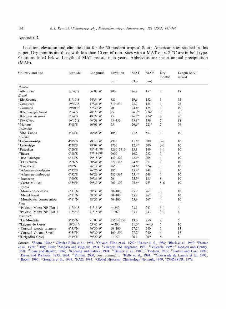
Appendix 2

Location, elevation and climatic data for the 30 modern tropical South American sites studied in thispaper. Dry months are those with less than 10 cm of rain. Sites with a MAT of 9 21‡C are in bold type.Citations listed below. Length of MAT record is in years. Abbreviations: mean annual precipitation(MAP).

Country and site Latitude Longitude Elevation MAT MAP Drymonths

Length MATrecord

(m) (‡C) (cm)

Bolivia1Alto Ivan 11‡45PS 66‡02PW 200 26.8 157 7 18Brazil2Rio Grande 21‡10PS 44‡54PW 825 19.6 152 5 323Conquista 19‡59PS 47‡36PW 510^530 23.7 155 6 264Corumba¤ 19‡01PS 57‡39PW 90 24.6a 125 6 105Bele¤mîgapo¤ forest 1‡54PS 48‡29PW 25 26.2b 274a 0 265Bele¤m^terra ¢rme 1‡54PS 48‡29PW 25 26.2b 274a 0 264Rio Claro 16‡16PS 56‡38PW 75^150 25.8b 139 6 886Manaus 3‡08PS 60‡01PW 75 26.6b 221a 2 76Colombia7Alto Yunda 3‡32PN 76‡48PW 1050 21.5 553 0 10Ecuador8Loja^non-ridge 4‡05PS 79‡10PW 2900 11.5a 300 0^1 108Loja^ridge 4‡28PS 79‡09PW 2700 12.4a 300 0^1 109Pasochoa 0‡29PS 78‡ 41PW 3260^3310 13.8 149 0^1 1010Baeza 0‡28PS 77‡ 54PW 2000 16.2 232 0 811Rio Palenque 0‡33PS 79‡18PW 150^220 22.1a 265 6 1012El Pechiche 1‡26PS 80‡41PW 320^365 24.8a 65 8 1013Cuyabeno 0‡0PS 76‡12PW 265 24.6a 324 0 1014An‹anagu^£oodplain 0‡32PS 76‡26PW 285 25.4a 248 0 1014An‹anaguûn£ooded 0‡32PS 76‡26PW 285^365 25.4a 248 0 1015Jauneche 1‡20PS 79‡35PW 70 25.3a 185 8 1016Cerro Mutiles 0‡54PN 79‡37PW 200^300 25.5a 75a 5^6 10Guyana17Mora consociation 6‡11PN 58‡37PW 50^100 25.9 267 0 1017Mixed forest 6‡11PN 58‡37PW 50^100 25.9 267 0 1017Morabukea consociation 6‡11PN 58‡37PW 50^100 25.9 267 0 10Peru18Pakitsa, Manu NP Plot 1 11‡56PS 71‡15PW V340 23.1 243 0^1 418Pakitsa, Manu NP Plot 3 11‡56PS 71‡15PW V360 23.1 243 0^1 4Venezuela19La Montan‹a 8‡35PN 71‡07PW 2550^2650 13.0 250 2 520Laguna de Cocos 10‡30PN 63‡45PW V200 21.0a V65 5 1021Corozal^woody savanna 6‡55PN 66‡30PW 90^100 27.2c 240 6 1321Corozal^Guiana Shield 6‡55PN 66‡30PW 100^500 27.2c 240 6 1322Delgadito Creek 8‡49PN 69‡29PW V150 26.1 209 5 6

Sources: 1Boom, 1986; 2 Oliveira-Filho et al., 1994; 3Oliveira-Filho et al., 1997; 4Ratter et al., 1988; 5Black et al., 1950; 6Pranceet al., 1976; 7Hilty, 1980; 8Madsen and Xllgaard, 1994; 9Valencia and JYrgensen, 1992; 10Valencia, 1995; 11Dodson and Gentry,1978; 12Josse and Balslev, 1994; 13Korning and Balslev, 1994; 14Balslev et al., 1987; 15Dodson, 1985; 16Parker and Carr, 1992;17Davis and Richards, 1933, 1934; 18Pitman, 2000, pers. commun.; 19Kelly et al., 1994; 20Guevarade de Lampe et al., 1992;21Boom, 1990; 22Stergios et al., 1998; aFAO, 1985; bGlobal Historical Climatology Network, 1999; cCODESUR, 1979.

PALAEO 2945 8-11-02


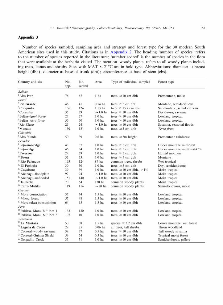
Appendix 3

Number of species sampled, sampling area and strategy and forest type for the 30 modern SouthAmerican sites used in this study. Citations as in Appendix 2. The heading ‘number of species’ refersto the number of species reported in the literature; ‘number scored’ is the number of species in the £orathat were available at the herbaria visited. The mention ‘woody plants’ refers to all woody plants includ-ing trees, lianas and shrubs. Sites with MAT 9 21‡C are in bold type. Abbreviations: diameter at breastheight (dbh); diameter at base of trunk (dbt); circumference at base of stem (cbs).

Country and site No.spp.

No.scored

Area Type of individual sampled Forest type

Bolivia1Alto Ivan 76 67 1 ha trees v 10 cm dbh Premontane, moistBrazil2Rio Grande 46 41 0.54 ha trees v 5 cm dbt Montane, semideciduous3Conquista 136 124 1.13 ha trees v 15.7 cm cbs Submontane, semideciduous4Corumba¤ 35 29 V1.0 ha trees v 10 cm dbh Deciduous, savanna5Bele¤mîgapo¤ forest 27 27 1.0 ha trees v 10 cm dbh Lowland tropical5Bele¤m^terra ¢rme 56 50 1.0 ha trees v 10 cm dbh Lowland tropical4Rio Claro 25 24 V1.0 ha trees v 10 cm dbh Savanna, seasonal £oods6Manaus 150 131 1.0 ha trees v 5 cm dbh Terra ¢rmeColombia7Alto Yunda 50 39 0.6 ha trees v 3m height Premontane rainforestEcuador8Loja^non-ridge 43 37 1.0 ha trees v 5 cm dbh Upper montane rainforest8Loja^ridge 46 34 1.0 ha trees v 5 cm dbh Upper montane rainforest/Cs9Pasochoa 29 29 1.0 ha trees v 5 cm dbh Humid montane10Baeza 33 33 1.0 ha trees v 5 cm dbh Montane11Rio Palenque 163 124 87 ha common trees, shrubs Wet tropical12El Pechiche 30 30 1.0 ha trees v 5 cm dbh Dry, semideciduous13Cuyabeno 39 39 1.0 ha trees v 10 cm dbh, s 1% Moist tropical14An‹anagu^£oodplain 97 94 V1.0 ha trees v 10 cm dbh Moist tropical14An‹anaguûn£ooded 151 140 V1.0 ha trees v 10 cm dbh Moist tropical15Jauneche 70 64 130 ha common woody plants Moist tropical16Cerro Mutiles 119 114 V20 ha common woody plants Semi-deciduous, moistGuyana17Mora consociation 37 34 1.5 ha trees v 10 cm dbh Lowland tropical17Mixed forest 57 48 1.5 ha trees v 10 cm dbh Lowland tropical17Morabukea consociation 64 55 1.5 ha trees v 10 cm dbh Lowland tropicalPeru18Pakitsa, Manu NP Plot 1 133 130 1.0 ha trees v 10 cm dbh Lowland tropical18Pakitsa, Manu NP Plot 3 107 101 1.0 ha trees v 10 cm dbh Lowland tropicalVenezuela19La Montan‹a 50 38 1.5 ha species v 3.2 cm dbh Lower montane, wet forest20Laguna de Cocos 29 25 0.06 ha all trees, tall shrubs Thorn woodland21Corozal^woody savanna 39 37 0.5 ha trees v 10 cm dbh Tall woody savanna21Corozal^Guiana Shield 59 54 0.5 ha trees v 10 cm dbh Tropical moist forest22Delgadito Creek 35 31 1.0 ha trees v 10 cm dbh Semideciduous, gallery

PALAEO 2945 8-11-02


References

Bailey, I., Sinnott, E., 1915. A botanical index of Cretaceousand Tertiary climates. Science 41, 831^834.

Bailey, I., Sinnott, E., 1916. The climatic distribution of certaintypes of angiosperm leaves. Am. J. Bot. 3, 24^39.

Balslev, H., Luteyn, J., Xllgaard, B., Holm-Nielsen, L., 1987.Composition and structure of adjacent un£ooded and £ood-plain forest in Amazonian Ecuador. Opera Bot. 92, 37^57.

Barnes, R.W., Jordan, G., Hill, R.S., McCoull, C.J., 2000. Acommon boundary between distinct northern and southernmorphotypes in two unrelated Tasmanian rainforest species.Aust. J. Bot. 48, 481^491.

Black, G., Dobzhansky, T., Pavan, C., 1950. Some attempts toestimate species diversity and population density of trees inAmazonian forests. Bot. Gaz. 111, 413^425.

Bongers, F., Popma, J., 1990. Leaf characteristics of the trop-ical rain forest £ora of Los Tuxtlas. Mex. Bot. Gaz. 151,354^365.

Boom, B., 1986. A forest inventory in Amazonian Bolivia.Biotropica 18, 287^294.

Boom, B., 1990. Flora and vegetation of the Guayana^Llanosecotone in Estado Bol|¤var, Venezuela. Mem. N.Y. Bot.Gard. 64, 254^278.

Burnham, R.J., 1994. Patterns in tropical leaf litter and impli-cations for angiosperm paleobotany. Rev. Palaeobot. Paly-nol. 81, 99^113.

Burnham, R.J., 1997. Stand characteristics and leaf litter com-position of a dry forest hectare in Santa Rosa NationalPark, Costa Rica. Biotropica 29, 384^395.

Burnham, R., Graham, A., 1999. The history of neotropicalvegetation: new developments and status. Ann. Mo. Bot.Gard. 86, 546^589.

Burnham, R.J., Pitman, N., Johnson, K., Wilf, P., 2001. Hab-itat-related error in estimating temperatures from leaf mar-gins in a humid tropical forest. Am. J. Bot.

CODESUR. 1979. Atlas de la regio¤n sur. Ministerio del Am-biente y de los Recursos Naturales Renovables, Direccio¤nGeneral de Informacio¤n e Investigacio¤n del Ambiente, Ca-racas. 67 pp.

Davis, T.A.W., Richards, P.W., 1933. The vegetation of Mora-balli Creek, British Guiana: An ecological study of a limitedarea of tropical rainforest, Part I. J. Ecol. 21, 350^384.

Davis, T.A.W., Richards, P.W., 1934. The vegetation of Mora-balli Creek, British Guiana: An ecological study of a limitedarea of tropical rainforest, Part II. J. Ecol. 22, 106^155.

Guevarade de Lampe, M., Bergeron, Y., McNeil, R., Leduc,A., 1992. Seasonal £owering and fruiting patterns in tropicalsemi-arid vegetation of northeastern Venezuela. Biotropica24, 64^76.

Dodson, C., 1985. La £ora de Jauneche, Los Rios, Ecuador.Banco Central del Ecuador, Quito.

Dodson, C., Gentry, A., 1978. Flora of the Rio Palenque Sci-ence Center. Selbyana 4, 1^6.

Food and Agriculture Organization of the United Nations,1985. Agroclimatological Data for Latin America and the

Caribbean. FAO Plant Production and Protection Series 24,Rome.

Gentry, A., 1996. A Field Guide to the Families and Genera ofWoody Plants of Northwest South America (Colombia,Ecuador, Peru) with Supplementary Notes on HerbaceousTaxa. The University of Chicago Press, Chicago, pp. 533^545.

Givnish, T., 1987. Comparative studies of leaf form: Assessingthe relative roles of selective pressures and phylogenetic con-straints. New Phytol. 106, 131^160.

Global Historical Climatology Network. 1999. National Cli-matic Data Center, Arizona State University and CarbonDioxide Information Analysis Center at Oak Ridge Nation-al Laboratory, Version 2, 1999 (http://dss.ucar.edu/datasets/ds546.0/).

Graham, A., 1995. Development of a⁄nities between Mexican/Central American and Northern South American Lowlandand Lower Montane vegetation during the Tertiary. In:Churchill, S.P., et al., Biodiversity and Conservation of Neo-tropical Montane Forests, pp. 11^22.

Greenwood, D., 1992. Taphonomic considerations on foliarphysiognomic interpretations of Late Cretaceous and Terti-ary palaeoclimates. Rev. Paleobot. Palynol. 71, 149^190.

Greenwood, D., 2001. Climate^wood and leaves, Section 4.3.6.In: Briggs, D.E., Crowther, P.R. (Eds.), Palaeobiology II.Blackwell Scienti¢c, London.

Gregory, K., 1994. Palaeoclimate and palaeoelevation of the35 Ma Florissant Flora, Front Range, Colorado. Palaeocli-mates 1, 23^57.

Gregory, K., Chase, C., 1992. Tectonic signi¢cance of paleo-botanically estimated climate and altitude of the Late Eo-cene erosion surface, Colorado. Geology 20, 581^585.

Gregory, K., McIntosh, W., 1996. Paleoclimate and paleoele-vation of the Oligocene Pitch-Pinnacle Flora, SawatchRange, Colorado. GSA Bull. 108, 545^561.

Gregory-Wodzicki, K., 2000. Relationships between leaf mor-phology and climate, Bolivia: Implications for estimatingpaleoclimate from fossil £oras. Paleobiology 26, 668^688.

Halloy, S., Mark, A., 1996. Comparative leaf morphologyspectra of plant communities in New Zealand, the Andesand the European Alps. J. R. Soc. N.Z. 26, 41^78.

Hilty, S., 1980. Flowering and fruiting periodicity in a premon-tane rain forest in Paci¢c Colombia. Biotropica 12, 292^306.

Jacobs, B., 1999. Estimation of rainfall variables from leafcharacters in tropical Africa. Palaeogeogr. Palaeoclimatol.Palaeoecol. 145, 231^250.

Jacobs, B., Deino, A., 1996. Test of climate^leaf physiognomyregression models, their application to two Miocene £orasfrom Kenya, and 40Ar/39Ar dating of the Late MioceneKapturo site. Palaeogeogr. Palaeoclimatol. Palaeoecol. 123,259^271.

Jordan, G., 1997. Uncertainty in paleoclimatic reconstructionsbased on leaf physiognomy. Aust. J. Bot. 45, 527^547.

Josse, C., Balslev, H., 1994. The composition and structure ofa dry, semideciduous forest in western Ecuador. Nord. J.Bot. 14, 425^434.

Kappelle, M., Leal, M., 1996. Changes in leaf morphology and

PALAEO 2945 8-11-02


foliar nutrient status along a successional gradient in a Cos-ta Rican upper montane Quercus forest. Biotropica 28, 331^344.

Kelly, D., Tanner, E., NicLughadha, E., Kapos, V., 1994.Floristics and biogeography of a rain forest in the Venezue-lan Andes. J. Biogeogr. 21, 421^440.

Korning, J., Balslev, H., 1994. Growth and mortality of treesin Amazonian tropical rain forest in Ecuador. J. Veg. Sci. 5,77^86.

Leigh, E.G., 1999. Tropical Forest Ecology: A view from Bar-ro Colorado Island. Oxford University Press, New York,pp.107^112.

Li, X., 1981. A Bibliography of Chinese Paleobotany. Instituteof Geology and Palaeontology, Academia Sinica, Nanjing.

Madsen, J., Xllgaard, B., 1994. Floristic composition, struc-ture, and dynamics of an upper montane rain forest insouthern Ecuador. Nord. J. Bot. 14, 403^423.

Oliveira-Filho, A., Vilela, E., Carvalho, D., Gavilanes, M.,1994. E¡ects of soils and topography on the distributionof tree species in a tropical riverine forest in south-easternBrazil. J. Trop. Ecol. 10, 483^508.

Oliveira-Filho, A., Curi, N., Vilela, E., Carvalho, D., 1997.Tree species distributions along soil catenas in a riversidesemideciduous forest in southeastern Brazil. Flora 192, 47^64.

Parker, T.A., Carr, J.L. (Eds.), 1992. Status of Forest Rem-nants in the Cordillera de la Costa and Adjacent Areas ofSouthwestern Ecuador. Conservation International, RAPWorking Papers 2.

Parkhurst, D., Loucks, O., 1972. Optimal leaf size in relationto environment. J. Ecol. 60, 505^537.

Pitman, N., 2000. A Large-Scale Inventory of Two AmazonianTree Communities. Ph.D. Thesis, Duke University, Dur-ham, NC.

Povey, D., Spicer, R., England, P., 1994. Paleobotanical inves-tigation of early Tertiary palaeoelevations in northeasternNevada: Initial results. Rev. Palaeobot. Palynol. 81, 1^10.

Prance, G., Rodrigues, W., da Silva, M., 1976. Inventa¤rio £o-restal de um hectare de mata de terra ¢rme km 30 da Es-trada ManausÎtacoatiara. Acta Amaz. 6, 9^35.

Ratter, J., A. Pott, Vali,J., Pott, J., da Cunha, C., Haridasan,M., 1988. Observations on woody vegetation types in thePantanal and at Corumba¤, Brazil .. Notes R. Bot. Gard.Edinb. 45, 503^525.

Sokal, R.R., Rohlf, F.J., 1995. Biometry, 3rd. ed. Freeman,New York, 498 pp.

Stergios, B., Comiskey, J., Dallmeier, F., Licata, A., Nin‹o, M.,1998. Species diversity, spatial distribution and structuralaspects of semi-deciduous lowland gallery forests in thewestern Llanos of Venezuela. In: Dallmeier, Cominsky,(Eds.), Forest Biodiversity in North, Central and SouthAmerica, and the Caribbean. Parthenon, New York, pp.449^479.

Stranks, L., England, P., 1997. The use of resemblance func-

tion in the measurement of climatic parameters from thephysiognomy of woody dicotyledons. Palaeogeogr. Palaeo-climatol. Palaeoecol. 131, 15^28.

ter Braak, C., 1991. CANOCO ^ A Fortran program for ca-nonical correspondence ordination. Microcomputer Power,Ithaca, NY (on disk).

Uhl, D., Mosbrugger, V., 1999. Leaf venation density as aclimate and environmental proxy: A critical review andnew data. Palaeogeogr. Palaeoclimatol. Palaeoecol. 149,15^26.

Valencia, R., 1995. Composition and structure of an Andeanforest fragment in eastern Ecuador. In: Churchill et al.(Eds.), Biodiversity and Conservation of Neotropical Mon-tane Forests. New York Botanical Garden, New York, pp.239^249.

Valencia, R., JYrgensen, P., 1992. Composition and structureof a humid montane forest on the Pasochoa Volcano, Ecua-dor. Nord. J. Bot. 12, 239^247.

Watson, L., Dallwitz, M.J., 1992. The Families of FloweringPlants: Descriptions, Illustrations, Identi¢cation, and Infor-mation Retrieval. Version: 14th December 2000 (http://bio-diversity.uno.edu/delta/’).

Wiemann, M., Manchester, S., Dilcher, D., Hinojosa, L.,Wheeler, E., 1998. Estimation of temperature and precipita-tion from morphological characters of dicotyledonousleaves. Am. J. Bot. 85, 1796^1802.

Wijninga, V., 1995. A ¢rst approximation on montane forestdevelopment during the Late Tertiary in Colombia. In:Churchill et al. (Eds.), Biodiversity and Conservation ofNeotropical Montane Forests. New York Botanical Garden,New York, pp. 23^34.

Wilf, P., 1997. When are leaves good thermometers? A NewCase for Leaf Margin Analysis. Paleobiology 23, 373^390.

Wing, S., Greenwood, D., 1993. Fossils and fossil climate: Thecase for equable continental interiors in the Eocene. Philos.Trans. R. Soc. Lond. B 341, 243^252.

Wolfe, J., 1971. Tertiary climatic £uctuations and methods ofanalysis of Tertiary £oras. Palaeogeogr. Palaeoclimatol. Pa-laeoecol. 9, 27^57.

Wolfe, J., 1978. A paleobotanical interpretation of Tertiaryclimates in the Northern Hemisphere. Am. Sci. 66, 694^703.

Wolfe, J., 1979. Temperature Parameters of Humid to MesicForests of Eastern Asia and Relation to Forests of OtherRegions in the Northern Hemisphere and Australasia. U.S.Geological Survey Professional Paper 1106, 37 pp.

Wolfe, J., 1993. A Method of Obtaining Climatic Parametersfrom Leaf Assemblages. U.S. Geological Survey Bulletin2040, 71 pp.

Wolfe, J., 1995. Paleoclimatic estimates from Tertiary leaf as-semblages. Ann. Rev. Earth Planet. Sci. 23, 119^142.

Wolfe, J., Spicer, R., 1999. Fossil leaf character states: Multi-variate analyses. In: Jones, T., Rowe, N. (Eds.), FossilPlants and Spores. The Geological Society, London, pp.233^239.

PALAEO 2945 8-11-02


Documents

Mean annual temperature estimation based on leaf ...ekowalsk/Kowalski.pdfMean annual temperature estimation based on leaf morphology: a test from tropical South America Elizabeth A