United States Environmental Protection Agency

Office of Water Office of Science and Technology Washington, DC 20460

EPA-822-R-08-023 December 2008 www.epa.gov

Methods for evaluating Wetland Condition

#19 Nutrient Loading

Major Contributors

Iowa State University U. Sunday Tim and William Crumpton

Prepared jointly by:

The U.S. Environmental Protection Agency Health and Ecological Criteria Division (Office of Science and Technology)

and

Wetlands Division (Office of Wetlands, Oceans, and Watersheds)

United States Environmental Protection Agency

Office of Water Office of Science and Technology Washington, DC 20460

EPA-822-R-08-023 December 2008 www.epa.gov

Methods for evaluating Wetland Condition

#19 Nutrient Loading

i i i

Notice

The material in this document has been subjected to U.S. Environmental Protection Agency (EPA) technical review and has been approved for publication as an EPA document. The information contained herein is offered to the reader as a review of the “state of the science” concerning wetland bioassessment and nutrient enrichment and is not intended to be prescriptive guidance or firm advice. Mention of trade names, products or services does not convey, and should not be interpreted as conveying official EPA approval, endorsement, or recommendation.

Appropriate Citation

U.S. EPA. 2008. Methods for Evaluating Wetland Condition: Nutrient Loading. Office of Water, U.S. Environmental Protection Agency, Washington, DC. EPA-822-R-08-023.

Acknowledgements

EPA acknowledges the contributions of the following people in the writing of this module: U. Sunday Tim and William Crumpton both of Iowa Sate University.

This entire document can be downloaded from the following U.S. EPA websites:

http://www.epa.gov/water science/criteria/wetlands/

http://www.epa.gov/owow/wetlands/bawwg/publicat.html

i v

Contents

foreWord � � � � � � � � � � � � � � � � � � � � � � � � � � � � � � � � � � � � � � v

list of “Methods for evaluating Wetland Condition” Modules � � � � � � � � � � � � � � � � � � � � � � � � �vi

nutrient loading � � � � � � � � � � � � � � � � � � � � � � � � � � � � � � � � �1

suMMary� � � � � � � � � � � � � � � � � � � � � � � � � � � � � � � � � � � � � � �1

PurPose � � � � � � � � � � � � � � � � � � � � � � � � � � � � � � � � � � � � � � �1

introduCtion � � � � � � � � � � � � � � � � � � � � � � � � � � � � � � � � � � � �1

loading funCtion Models � � � � � � � � � � � � � � � � � � � � � � � � � � � �2

ProCess-oriented Models � � � � � � � � � � � � � � � � � � � � � � � � � � � �7

liMitations and Model validation � � � � � � � � � � � � � � � � � � � � � � �25

Choosing a suitable Model � � � � � � � � � � � � � � � � � � � � � � � � � � 31

referenCes � � � � � � � � � � � � � � � � � � � � � � � � � � � � � � � � � � � �34

list of tables

table 1: inPut ParaMeters required by gWlf Model � � � � � � � � � � � � �4

table 2: inPut ParaMeters required by agnPs Model � � � � � � � � � � � �8

table 3: inPut ParaMeters required by hsPf � � � � � � � � � � � � � � � � 15

table 4: sWat/sWat 200 inPut ParaMeters � � � � � � � � � � � � � � � 19

list of figures

figure 1: Model quality assuranCe CoMPonents � � � � � � � � � � � � � � 26

v

foreWord

In 1999, the U.S. Environmental Protection Agency (EPA) began work on this series of reports entitled Methods for Evaluating Wetland Condition. The purpose of these reports is to help States and Tribes develop methods to evaluate (1) the overall ecological condition of wetlands using biological assessments and (2) nutrient enrichment of wetlands, which is one of the pri-mary stressors damaging wetlands in many parts of the country. This information is intended to serve as a starting point for States and Tribes to eventually establish biological and nutrient water quality criteria specifically refined for wetland waterbodies.

This purpose was to be accomplished by providing a series of “state of the science” modules concerning wetland bioassessment as well as the nutrient enrichment of wetlands. The individual module format was used instead of one large publication to facilitate the addition of other reports as wetland science progresses and wetlands are further incorporated into water quality programs. Also, this modular approach allows EPA to revise reports without having to reprint them all. A list of the inaugural set of 20 modules can be found at the end of this section.

This last set of reports is the product of a collaborative effort between EPA’s Health and Ecological Criteria Division of the Office of Science and Technology (OST) and the Wetlands Division of the Office of Wetlands, Oceans and Watersheds (OWOW). The reports were initiated with the support and oversight of Thomas J. Danielson then of OWOW, Amanda K. Parker and Susan K. Jackson (OST), and seen to completion by Ifeyinwa F. Davis (OST). EPA relied on the input and expertise of the contributing authors to publish the remaining modules.

More information about biological and nutrient criteria is available at the following EPA website:

http://www.epa.gov/ost/standards

More information about wetland biological assessments is available at the following EPA website:

http://www.epa.gov/owow/wetlands/bawwg

v i

List of “Methods for evALuAtiNg WetLANd CoNditioN” ModuLes

Module # Module title

1 ����������������� introduCtion to Wetland biologiCal assessMent

2 ����������������� introduCtion to Wetland nutrient assessMent

3 ����������������� the state of Wetland sCienCe

4 ����������������� study design for Monitoring Wetlands

5 ����������������� adMinistrative fraMeWork for the iMPleMentation of a Wetland bioassessMent PrograM

6 ����������������� develoPing MetriCs and indexes of biologiCal integrity

7 ����������������� Wetlands ClassifiCation

8 ����������������� volunteers and Wetland bioMonitoring

9 ����������������� develoPing an invertebrate index of biologiCal integrity for Wetlands

10 ��������������� using vegetation to assess environMental Conditions in Wetlands

11 ��������������� using algae to assess environMental Conditions in Wetlands

12 ��������������� using aMPhibians in bioassessMents of Wetlands

13 ��������������� biologiCal assessMent Methods for birds

14 ��������������� Wetland bioassessMent Case studies

15 ��������������� bioassessMent Methods for fish

16 ��������������� vegetation-based indiCators of Wetland nutrient enriChMent

17 ��������������� land-use CharaCterization for nutrient and sediMent risk assessMent

18 ��������������� biogeoCheMiCal indiCators

19 ��������������� nutrient loading

20 �������������� Wetland hydrology

1

nutrient loading

T he purpose of this module is to describe and discuss the general hydrologic prop-

erties that make wetlands unique, and to pro-vide an overview of the processes that control wetland hydrologic behavior. The intent is to provide a general discussion of wetland hy-drologic processes and methods in the hope of fostering an understanding of the impor-tant attributes of wetland hydrology relevant to the monitoring and assessment of these systems. As such, it is not intended to address the narrower definition of wetland hydrology for jurisdictional or classification purposes. Also, this module should not replace more advanced wetland texts. If the need arises to obtain more specific information, the reader is advised to refer to wetland books or ar-ticles, including those referenced within this document.

suMMary

N utrient loading to wetlands is deter-mined primarily by surface and subsur-

face transport from the contributing land-scape, and varies significantly as a function of weather and landscape characteristics such as soils, topography, and land use. In the ab-sence of sufficient measurements, nutrient loading can only be estimated using an appro-priate loading model. This module provides an overview of hydrologic and contaminant transport models that can be used to estimate nutrient loads to wetlands.

PurPose

T he purpose of this module is to provide an overview of hydrologic and contami-

nant transport models that can be used to es-timate nutrient loads to wetlands.

introduCtion

Over the past three decades, considerable effort has been expended in developing

models to simulate watershed hydrology and nutrient transport, particularly the estima-tion of cumulative field/watershed contribu-tions of flow, sediment, nutrients, and other contaminants of interest. Appropriately used, existing models may apply when in evaluat-ing wetland reference conditions or establish-ing nutrient criteria for wetlands or guiding management decisions once nutrient criteria are established.

Several reviews have summarized the char-acteristics, features, strengths, and limitations of models that are used for estimating wa-tershed hydrology and water quality (Doni-gian, et al., et al. 1991b, 1995b; DeVries and Hromadka 1993; Novotny and Olem 1994; Tim 1996a, 1996b). These models vary wide-ly in structure and in spatial and temporal scale, and can be classified as (i) empirical or semi-empirical loading function models and ii) process-oriented simulation models.

2

loading funCtion Models

Loading function models are based on em-pirical or semi-empirical relationships that

provide estimates of pollutant loads based on long-term measurements of flow and contam-inant concentration. They provide for rapid estimation of critical pollutant loads with minimal effort and data requirements. Load-ing function models are widely used to esti-mate pollutant loads in areas where limited data sets are available for process-based mod-eling. A major advantage of loading function models is their simplicity. Generally, loading function models contain procedures for esti-mating pollutant load based on either heuris-tics or on the empirical relationships between landscape physiographic characteristics and phenomena that control pollutant export.

McElroy et al. (1976) and Mills (1985) de-scribed components of several screening models developed by EPA’s Environmental Research Laboratory at Athens, Georgia to facilitate estimation of nutrient loads from point and nonpoint sources and to enhance preliminary assessment of water quality. The model con-tains simple empirical expressions that relate the magnitude of nonpoint pollutant load to readily available or measurable input param-eters such as soils, land use and land cover, land management practices, and topography. This model is attractive because it can be applied to very large watersheds often with minimal effort and little or no calibration is required.

Regression modeling, an approach based on statistical descriptions of historic flow and pollutant concentration data, is an alternative

to the screening model Regression models are used to obtain preliminary estimates of pollut-ant load under limiting and incomplete data. These models require primary input param-eters such as drainage area, percent impervi-ousness, mean annual precipitation, land use pattern, and ambient temperature. Regression models can determine storm-event mean pol-lutant load with confidence intervals for the estimated loads.

In addition to regression modeling, sever-al less complex, process-based models have been used to estimate flow and contaminant transport in terrestrial environments. Ex-amples of process-based models include the Generalized Watershed Loading Function (GWLF), the Spatially Referenced Regres-sions on Watersheds (SPARROW), and the Pollutant Load model (PLOAD).

geNerALized WAtershed LoAdiNg fuNCtioN ModeL

The Generalized Watershed Loading Func-tion Model (GWLF), developed at Cornell University, estimates stream flow, nutrient load and sediment load from watersheds management areas. The model allows simu-lation of point and nonpoint loadings of nu-trients and pesticides from urban and agricul-tural watersheds, including septic systems. The model also provides data to evaluate the effectiveness of certain land use management practices. The GWLF is a temporally-contin-uous simulation model with daily time steps, but it is not spatially distributed. It simulates overland flow and channel flow using a water balance approach based on measurements of daily precipitation and average temperature. Precipitation is partitioned into direct surface runoff and infiltration using the SCS Curve

3

Number technique. Here, the Curve Number determines the amount of precipitation that runs off directly, adjusted for antecedent soil moisture based on total precipitation dur-ing the previous five days. A separate Curve Number is specified for each combination of land use types and soil hydrologic groups. The amount of water available to the shallow groundwater zone is influenced by evapo-transpiration. This is estimated in GWLF us-ing the available moisture in the unsaturated zone, the evapo-transpiration potential, and a cover coefficient. Potential evapo-transpira-tion is estimated from a relationship to mean daily temperature and the number of daylight hours. GWLF calculates the groundwater dis-charge by performing a lumped parameter water balance on the saturated and shallow saturated zones.

Soil erosion is modeled by the Revised Uni-versal Soil-loss Equation (RULSE). Nutrient fluxes in GWLF are estimated empirically using daily nutrient fluxes from surface run-off from pervious and impervious surfaces, sediment erosion, groundwater base-flow, and septic runoff. The monthly nutrient load is calculated by totaling the daily nutrient fluxes. In GWLF, the nitrogen and phospho-rus loads from surface runoff are estimated by multiplying excess runoff by their flow-weight-ed average concentrations, respectively.

The model assumes that each specific land-cover type has unique event-mean-concen-tration processes that affect transport and storage, and are unique to the land use. The nutrient-loading model for urban land use is based on an accumulation/wash off model. Nutrient fluxes from impervious surfaces and urban lands are estimated using chemical build-up and wash-off parameterization. Both

nitrogen and phosphorus from eroded sedi-ments are estimated using the sediment load, enrichment ratio, and the concentration of nitrogen and phosphorus in the top layer of the soil. As with many mid-range terrestrial models, GWLF calculates concentrations of dissolved and sediment-bound nitrogen and phosphorus in stream flow as the sum total of base flow, stream flow (overland flow) and point sources. Groundwater only contributes dissolved nitrogen and phosphorus values re-flecting the effects of local land use. Nutri-ent losses in urban runoff are assumed to be entirely in the solid-phase, while point source losses are assumed to be dissolved.

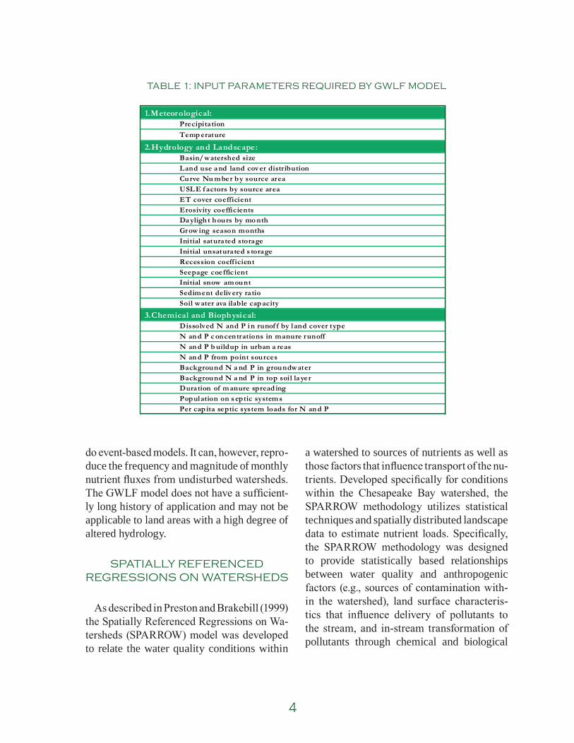
The GWLF requires three categories of input parameters: meteorological; hydrology and landscape; and chemical and biophysical (see Table 1). The model requires daily pre-cipitation and temperature. The GWLF also requires information related to land use, land cover, soil, and parameters that govern run-off, erosion, and nutrient load generation. The strength of GWLF model is that data required by this model are readily available from most resource management agency databases.

In general, GWLF is an empirically de-rived, statistically based process that uses daily inputs of precipitation and temperatures to compute nutrient fluxes. A major strength of GWLF is its simplicity in estimating pol-lutant load. Because of this, the model has been used for screening landscapes accord-ing to their pollutant delivery potentials or for identifying critical areas of nonpoint pollu-tion. However, it does not account for rainfall intensity or storage along channels. Because it uses a simplified technique for estimating base flow, the model cannot reproduce the precise history of overland flow and fluxes as

4

do event-based models. It can, however, repro-duce the frequency and magnitude of monthly nutrient fluxes from undisturbed watersheds. The GWLF model does not have a sufficient-ly long history of application and may not be applicable to land areas with a high degree of altered hydrology.

spAtiALLy refereNCed regressioNs oN WAtersheds

As described in Preston and Brakebill (1999) the Spatially Referenced Regressions on Wa-tersheds (SPARROW) model was developed to relate the water quality conditions within

a watershed to sources of nutrients as well as those factors that influence transport of the nu-trients. Developed specifically for conditions within the Chesapeake Bay watershed, the SPARROW methodology utilizes statistical techniques and spatially distributed landscape data to estimate nutrient loads. Specifically, the SPARROW methodology was designed to provide statistically based relationships between water quality and anthropogenic factors (e.g., sources of contamination with-in the watershed), land surface characteris-tics that influence delivery of pollutants to the stream, and in-stream transformation of pollutants through chemical and biological

tAbLe 1: iNput pArAMeters required by gWLf ModeL

1.Meteorological:PrecipitationTemp erature

2.Hydrology and Landscape:Basin/watershed sizeLand use a nd land cov er distributionCu rve Nu mber b y source areaUSL E f actors by source areaET cover coefficientErosivity coefficientsDa yligh t h ours by mo nthGrow ing season monthsInitial saturated storageInitial unsaturated s torageRecession coefficientSeepage coeffic ientInitial snow amountSediment delivery ratioSoil water ava ilable cap acity

3.Chemical and Biophysical:Dissolved N and P in runof f by land cover typeN an d P c oncentrations in manure runoffN an d P b uildup in urban a reasN an d P from point sourcesBackground N a nd P in groundwaterBackground N a nd P in top soil la yerDuration of manure spread ingPopulation on s eptic system sPer cap ita septic system loads for N an d P

5

pathways. The general form of the statistical regression model for SPARROW is (Preston and Brakebill 1999):

in which Li = nutrient load in stream reach i; n, N = pollutant source index; N = total number of sources; J(i) = number of upstream stream reaches; ßn = estimated source parameter; Sn,j = contaminant mass from source n in drainage to reach j; a = estimated vector of land-to-water delivery parameters; zj = land surface charac-teristics associated with drainage reach j (e.g., temperature, slope, stream density, irrigated land, precipitation, and wetland); d = estimated vector of in-stream loss parameter; and Ti,j = channel transport characteristics. The source parameter b consists of point sources, nutrient applications in the form of animal manure, commercial fertilizer, and atmospheric depo-sition of pollutants. The parameter, a, deter-mines the relative influence of different types of land-surface characteristics on the deliv-ery of nutrients from land surfaces to stream channels.

The literature reports a number of applica-tions of SPARROW model, primarily applied to the Chesapeake Bay ecosystem. These ar-ticles document water quality conditions and assess the effectiveness of best management practices in controlling nonpoint pollution. The results provided the basis for not only delineating watershed areas that are most critical to the export of nutrients, but also for targeting and prioritizing remedial control strategies and conservation programs (Smith, et al. 1997).

MidrANge ModeLs

In addition to the GWLF and SPARROW models described above, other modeling ap-proaches utilize a compromise between em-piricism and more complex mechanistic ap-proaches. Typical examples of such models include the Stormwater Intercept and Treat-ment Evaluation Model for Analysis and Planning (SITEMAP) (Omnicron Associates 1990) and Pollutant Load model or PLOAD. These models use daily time steps. Both can be used to examine seasonal variability and the load response to landscape characteristics of specific watersheds. Due to their complex-ity, they may have greater data requirements and may require more site-specific data.

SITEMAP is a dynamic simulation model developed to assist with simulating stream segment waste-load allocations from point and non-point sources. This model calculates daily runoff and pollutant loading and can be used for storm-event or continuous simula-tions (including probability distributions) of runoff, pollutant loads, infiltration, soil mois-ture, and evapo-transpiration. SITEMAP can be used in either single or mixed land uses, and for event-based or continuous simulation of surface runoff and pollutant load. Users of the model are able to assess the effectiveness of alternative management strategies and to estimate load and waste-load from point and nonpoint sources, respectively. The primary outputs from the model include probabilis-tic estimates of runoff volume and nutrient loadings. A typical example application of SITEMAP involved the assessment of pol-lutant load and surface runoff in the Tualatin River Basin and Fairview Creek watershed in Oregon.

L S z Ti n n j

j J in

N

j i j= − −∑∑=

β α δε

,

( )

,exp( ' ) exp( ' )1

6

PLOAD is a simplified GIS-based water-shed-loading model. It can model combined point and non-point source loads in either small urban areas or in rural watersheds of any size. As a loading model, PLOAD pro-vides annualized estimates of pollutant ex-port to waterbodies. Pollutants most com-monly analyzed include sediments (TSS and TDS), oxygen demand (BOD and COD), nu-trients (nitrogen, nitrate plus nitrite, TKN, ammonia, phosphorous), metals (lead, zinc) and bacteria (fecal coliform), or any other user-specified pollutant. The model addresses pollutant loading by land use categories and sub-watersheds, but does not as certain indi-vidual non-point sources or at actual pollut-ant fate and transport processes. Additional features of the model include: (i) the ability to estimate average annual pollutant load, (ii) a user-friendly interface that enhances manipu-lation of input parameters and the assessment of alternative pollution control strategies, (iii) tools to facilitate evaluation of land use change impacts, and (iv) the ability to gener-ate outputs at user-defined formats.

To use the PLOAD model, users are re-quired to provide reasonably accurate val-ues of input parameters describing wa-tershed land use and land cover, pollutant loading functions—based on land cover types, location of point source inputs, land areas with specified BMPs, and other gen-eral watershed characteristics. When sup-plied with these input variables, PLOAD generates outputs that include average an-nual loads, aggregated by sub-watershed, and reported in tables and maps of loads by watershed. In addition, users of PLOAD can view and compare multiple loading scenarios simultaneously.

The PLOAD is a part of the comprehensive modeling tools in the EPA’s Better Assess-ment Science Integrating Point and Nonpoint Sources (BASINS). The literature also re-ports the applications of the PLOAD model for assessing the effects of land use change and BMPs for watersheds in North Carolina and Maryland.

suMMAry of LoAdiNg fuNCtioN ModeLs

In summary, the many and diverse loading function models developed to allow estima-tion of point and non-point source pollution loads are based on simplistic, functional and empirical expressions that integrate flow and pollutant concentration. Attractive features of these models are that they: (i) require very limited data and computer modeling experi-ence; (ii) contain relatively simple procedures for estimating pollutant load; and, (iii) pro-vide tools for rapid assessment of point and non-point contributions to the watershed pol-lutant load. However, these advantages come at some expense regarding accuracy, nature of environmental process and conceptualization of the physical system. In particular, most loading function models fail to incorporate the complex, nonlinear biogeochemical and physical processes that influence the physical system. Furthermore, loading function mod-els are limited in how spatial and temporal processes are handled and how landscape variability is characterized. Despite these limitations, there are situations in which these models are logical and legitimate.

7

ProCess-oriented Models

I n contrast to the empirical and simplified loading function models described above,

process-oriented simulation models integrate knowledge of physical, chemical, and biologi-cal processes with empirical data, and allow users to evaluate interactions among human, economic and societal factors. This section provides an overview of some of the process-oriented simulation models that have been used to predict watershed hydrology and water quality, and that could provide mod-eling tools for predicting nutrient loading to wetlands. These models include AGNPS and AnnAGNPS, HEC-HMS, HEC-5Q, HSPF, STORM, SWAT, SWMM, and SWRRB models.

AgriCuLturAL NoNpoiNt sourCe ModeL

The Agricultural Non-Point Source Pollu-tion Model (AGNPS) is event-based, as well as a continuous or annualized AGNPS (An-nAGNPS) simulation model. These models predict surface runoff, sediment yield, and nutrient transport primarily from agricultur-al watersheds. The two main nutrients simu-lated are nitrogen and phosphorus, which are essential plant nutrients and are major con-tributors to eutrophication and surface water pollution. The basic model components include hydrology, erosion, sediment, and chemical transport (primarily nutrients and pesticides). The model also considers point sources of water, sediment, nutrients, and chemical oxy-gen demand (COD from various sources in-cluding feedlots). Water impoundments are also considered as depositional areas for sed-

iment-associated nutrients. The model also has the ability to output water quality charac-teristics at intermediate or user-defined points throughout the watershed stream network.

The AGNPS model uses a grid-cell-based subdivision of the watershed, in which each cell is considered homogeneous. The cells are linked together through the aspect or flow direction, and all watershed characteristics and primary biophysical inputs are expressed at the grid-cell level. The components of the model use equations and methodologies that have been well established in the water quality modeling literature and are extensively used by resource management agencies. For exam-ple, the runoff volume is estimated using the SCS curve number technique. The peak run-off rate for each grid-cell is estimated using an empirical relationship in the CREAMS mod-el (Knisel 1980). Soil erosion and sediment yield are computed by using the USLE and a bedload equation, a relationship—developed by Foster et al. (1981) based on the continuity equation. In the model, feedlots are treated as point sources and pollutant contributions from these sources are estimated by using the feedlot pollution model developed by Young (1982). Other point sources are accounted for by incorporating incoming flow rates and concentrations of nutrients to the cells where they occur.

In the AGNPS model, the resolution for the individual grid cells can range from 2.5 acres to greater than 40 acres (or 1 ha to more than 10 ha) depending on the problem being addressed, the size and complexity of the watershed, and the technical expertise of the modeler. Smaller grid-cell sizes such as 10 acres (4 ha) are recommended for water-shed less than 2000 acres (800 ha). However,

8

for watershed and catchments that are larger than 2000 acres (800 ha), grid-cell sizes of 40 acres (16 ha) are normally used. The calcula-tion of flow and transport processes in AG-NPS occurs in three stages based on a set of twenty or more parameters for each grid cell, with the initial calculations for all cells in the watershed made in the first stage. The sec-ond stage calculates the runoff volume and sediment yield for each of the cells contain-ing impoundments and the sediment yields for primary cells. A primary cell is one into which no other cell drains.

The non-point source pollution component of the model estimates transport and trans-formation of nitrogen, phosphorus, chemi-cal oxygen demand, and pesticides. Pollutant

transport is subdivided into soluble or dis-solved phase and the sediment-attached or sediment-bound phase. Soluble nitrogen and phosphorus compounds are calculated using a relationship adapted from the CREAMS model (Knisel 1980); along with sediment yield equations taken from the CREAMS and the WEPP models. The input parameters for the AGNPS model include: cell number, re-ceiving cell number, SCS curve number, land slope, field slope length, channel slope, chan-nel side-slope, soil erodibility factor, cover and management factor, support practice fac-tor, surface condition constant, aspect, and many other parameters related to land cover, land topography, management practices, and climate. The watershed-level parameters re-quired include: area, area of each grid-cell, characteristics of storm precipitation, and

Watershed-leve l Input Par ameters:Watershed identificationCe ll area (Ac res)Total numb er of grid cellsPrecipitation (inches)Energy-In tensityStorm type

Ce ll-level Input P arame ters:Ce ll numb erAspectSCS Curve Nu mberAve rage land s lope (°o)Slope shape factor (uniform, convex, concave)Ave rage field slope lengthMa nning roughness coeffic ientSoil erodibility factor (K-U SL E)Cropping f actor (C-USLE)Prac tice (P-USLE)Surface condition constantSoil texture (sand, silt, clay, peat)Fertilization levelFertilization ava ilability factorPoint source indicationGu lly source levelChemical oxygen demand factor

tAbLe 2: iNput pArAMeters required by AgNps ModeL

9

storm energy-intensity. Table 2 summarizes the major input parameters required by the AGNPS model.

The AGNPS model is, by far one of the more widely used water quality models for estimating the relative effects of agricultural management practices in small to large wa-tersheds. However, the model has many limi-tations, including: lack of process-level de-scription of nutrient transformation processes or the biochemical cycling of major plant ele-ments to document the biochemical cycling during transport; inability to characterize the transport and transformation of nutrients and pesticides in stream channels or similar waterbodies; inability to handle sub-surface flow and transport processes, as well as sub-surface interactions; the lack of a process to route flow or pollutants from individual grid-cells to the watershed outlet; and the model is event-based.

ANNuAL AgNps

To eliminate some of these limiting factors, the AGNPS model has undergone numerous refinements. The term “AGNPS” now refers to the system of modeling components instead of the single-event AGNPS described above. These enhancements made to the event-based AGNPS of the 1980s and early 1990s are in-tended to improve the capability of the pro-gram and to automate many of the input data preparation steps needed for use with large watershed systems. The current version of the model is called AnnAGNPS, which is virtu-ally the same computer program as AGNPS 5.x except that it allows for continuous simu-lations of surface runoff, peak flow rate, and pollutant transport for longer time periods and on a daily basis. AnnAGNPS is designed

to handle watershed areas of up to 300,000 ha, and it divides the watershed area into sub-divisions of homogenous cells with respect to soil type, land use, and land management.

In contrast to the event-based model, AnnAGNPS operates on a daily time step. It simulates water, sediment, nutrients, and pesticide transport at the cell and watershed levels. Special components are included to handle concentrated sources of nutrients from feedlots and point sources, concentrat-ed sediment sources with attached chemicals from gullies, and irrigation (water with dis-solved chemicals and sediment with attached chemicals). Each day the applied water and resulting runoff are routed through the wa-tershed system before the next day is consid-ered. The model partitions soluble nutrients and pesticides between surface runoff and infiltration. Sediment-transported nutrients and pesticides are estimated and equilibrated within the stream system, with the sediment assumed to consist of five particle size class-es (clay, silt, sand, small aggregate, and large aggregate).

The soil profile is divided into two layers. For estimating surface runoff, infiltration and soil water storage. The top 200 mm are used as a tillage layer whose properties can change; the second layer’s properties remain static. A daily soil moisture water budget con-siders applied water (rainfall, irrigation, and snowmelt), runoff, evapo-transpiration, and percolation. Surface runoff is estimated by using the SCS Runoff Curve Number equa-tion where the Curve Number can be modi-fied daily, based on tillage operations, soil moisture, and crop stage. Evapotranspiration is estimated as a function of potential evapo-transpiration by using the Penman equation

10

(Penman 1948) and soil moisture content. Erosion and sediment transport is predicted within a watershed landscape according to RUSLE (Renard, et al. 1997).

For each day and each grid cell, the model calculates mass balances of nutrients (pri-marily nitrogen, phosphorous), and organic carbon. The model considers plant uptake of nitrogen and phosphorus, fertilization, resi-due decomposition, and nutrient transport. Soluble and sediment-adsorbed nutrients are estimated, and they are further partitioned into organic and mineral phases. Each nu-trient component is decayed based upon the reach travel time, water temperature, and appropriate decay-constant. The soluble nu-trients are decreased further by infiltration. Attached nutrients are adjusted for deposition of clay particles Based on a first-order rela-tionship, equilibrium concentrations are cal-culated at both the upstream and downstream points of reach. Plant uptake of nutrients is modeled through a simple crop growth stage index. A daily mass balance adapted from GLEAMS (Leonard , et al. 1987) is estimated for each pesticide. The pesticides have unique chemodynamic properties, including half-life and organic matter partitioning coefficient. Major components of the pesticide model in-clude foliage wash-off, vertical transport in the soil profile, and degradation. Soluble and sediment adsorbed fractions are calculated for each grid cell on a daily basis.

AnnAGNPS also contains simplified meth-ods to route sediment, nutrients, and pesti-cides through the watershed. Peak flow for each reach is calculated using an extension of the TR-55 graphical peak-discharge method. Sediment routing is calculated based upon transport capacity relationships using the

Bagnold stream power equation. Sediments are routed by particle size class, where each particular size class can be deposited, more entrained, or transported unchanged; de-pending upon the amount entering the reach, the availability of that size class in the chan-nel and banks, and the transport capacity of each size class. If the sum of all incoming sediment is greater than the sediment trans-port capacity, then the sediment is deposited. If that sum is less than the sediment trans-port capacity, the sediment discharge at the downstream end of the reach will include bed and bank material (if it is an erodible reach). Nutrients and pesticides are subdivided into soluble and sediment attached components for routing. Attached phosphorus is further subdivided into organic and inorganic. Each nutrient component is decayed based upon the reach travel time, water temperature, and appropriate decay constant. Soluble nutrients are further reduced by infiltration. Attached nutrients are adjusted for deposition of clay particles. Based on a first-order relationship, equilibrium concentrations are calculated at both the upstream and downstream points of the reach.

AnnAGNPS includes 34 different input data categories, which can be grouped into climate, landscape characterization, agricul-tural management, chemical characteristics, and feedlot operations. The climatic data con-sist of precipitation, maximum and minimum air temperature, relative humidity, sky cover, and wind speed. Land characterization data include soil characterization, curve number, RUSLE parameters, and watershed drainage characterization. Agricultural management relates to data on tillage, planting, harvest, rotation, chemical operations, and irrigation schedules. Feedlot operations include daily

11

manure production rates, times of manure re-moval, and residual amount from previous op-erations. Indeed, there are over 400 separate input parameters necessary for model execu-tion. Some of these parameters are repeated for each cell, soil type, land use, feedlot, and/or channel reach. Separate parameters are necessary for the model verification section. Default values are available for some of the input parameters. The daily climate data in-put set includes twenty-two parameters, eight of which are repeated for each day simulat-ed. A climate generator, GEM, can be used to generate the precipitation and minimum/maximum air temperatures for AnnAGNPS. The development of other input data can be simplified because of duplication over a given watershed. Some of the geographical inputs including cell boundaries, land slope, slope direction, and land use, can be generated by GIS and digital elevation models. Model in-put is facilitated by an input editor, which is currently available with the model. The input editor interface provides a page format for data input, with each of the 34 major data cat-egories on a separate input page. Input and output can be in either all English or all met-ric units. Separate input files for watershed and climate data allow for quickly changing climatic input.

Extensive data checks (with appropriate er-ror messages) are performed as data are en-tered and, to a lesser extent, after all data are read. Output is expressed on an event basis for selected stream channel reaches and as source accounting from land or reach com-ponents over the simulation period. Primary outputs parameters generated by the model relate to soluble and attached sediment-nu-trients and pesticides, surface runoff volume and peak flow, and sediment yield based on

particle size classes. Each output parameters can be selected by the user for the desired wa-tershed source locations (specific cells, reach-es, feedlots, point sources, and gullies) and for any simulation period. Source accounting indicates the fraction of a pollutant load pass-ing through any reach in the stream network that came from the user-identified watershed source location. In addition, event quantities for user-selected parameters can be extracted at desired stream reach locations.

A major limitation of the AnnAGNPS is that it does not estimate transport of pesticide me-tabolites or daughter products. Other limita-tions of AnnAGNPS models include: (1) they lack a nutrient transformation component for both nutrient, and pesticides; (2) they lack a subsurface or near-surface water flow com-ponents; (3) they lack flow and contaminant routing component; (4) all runoff and associ-ated pollutant (sediment, nutrient, and pesti-cide) loads for a single day are routed to the watershed outlet before the next day simula-tion begins (regardless of how many days this may actually take); (5) there are no mass bal-ance calculations tracking inflow and outflow of water; (6) there is no tracking of sediment-bound pollutants in the stream reaches; (7) point sources are limited to constant loading rates (water and nutrients); and, (8) there is no provision for using spatially variable rainfall inputs. Detailed information on AGNPS and AnnAGNPS can be found at http://www.sed-lab.olemiss.edu/PLM/ AnnAGNPS.html.

hydroLogiC eNgiNeeriNg CoMputAtioN- hydroLogiC

ModeLiNg systeM

The Hydrologic Engineering Computation – Hydrologic Modeling System or HEC-HMS,

12

developed by the U.S. Army Corps of Engi-neers, is a physically-based model designed to simulate precipitation runoff processes of den-dritic watersheds. The model was developed to allow the simulation of large river basins and flood hydrology, as well as small urban watersheds. HEC-HMS is the latest version of the HEC-1 model and exhibits a number of similar options for simulating precipitation-runoff processes. In addition to unit hydro-graphic and hydrologic routing functions, ca-pabilities available with HEC-HMS include a linear-distributed runoff transformation that can be applied with gridded rainfall data, a simple “moisture-depletion” option that can be used for simulations over extended time periods, and a versatile parameter optimiza-tion option.

HEC-HMS also provides the capability for continuous soil moisture accounting and res-ervoir routing operations. Several options are included in HEC-HMS to compute overland flow and infiltration. These include the SCS Curve Number equation, gridded SCS Curve Number equation, and the Green-Ampt equa-tion. In addition to unit hydrographic and hydrologic routing options, other capabilities of the model include: linear quasi-distributed runoff transformation for use with gridded precipitation and terrain data such as DEM; continuous simulation with either one layer or a more complex five layer soil moisture meth-od; and, a versatile parameter estimation op-tion. The modified Clark method, ModClark, is a linear quasi-distributed unit hydrograph method that can be applied with gridded pre-cipitation. A variety of flow routing schemes are included in the model. Hydrographs pro-duced by the model can be used directly or in conjunction with other model for studies of water quality, urban drainage, flow forecasting,

reservoir spillway design, flood mitigation, and flood management.

The HEC-HMS modeling environment has been enhanced by geospatial technologies. For example, the GEOspatial Hydrologic Modeling Extension or HEC-GEOHMS is a software package that integrates HEC-HMS with ArcView GIS. GEOHMS also incor-porates ArcView Spatial Analyst Extension to allow users to generate model inputs for HEC-HMS. Using the digital terrain data from GIS databases, HEC-GEOHMS trans-forms the drainage paths and watershed boundaries into a hydrologic data structure that represents watershed response to precipi-tation. It provides an integrated, spatially-ex-plicit simulation environment with data man-agement and customized toolkit capabilities. Other interactive capabilities allow users to construct a hydrologic schematic of the wa-tershed at stream gages, hydraulic structures, and control points within the waterbody.

HEC-HMS also features a Windows-based graphical user interface (GUI), integrated hy-drological analysis components, data storage and management capabilities, and graphics and reporting tools. The data storage and ma-nipulation component is used for the storage and retrieval of time series, paired functions, and gridded data, in a manner that is largely transparent to the user. The HEC-HMS GUI provides a means for specifying watershed components, inputting data for each compo-nent, and examining the results interactively. It also contains global editors for entering or examining data for all applicable landscape elements.

Both HEC-HMS and HEC-GEOHMS have long history of application as a quasi-

13

dynamic hydrologic model. They are both in the public domain and their technical refer-ence manuals contain useful information on how to model hydrological processes in gen-eral, and the implementation of HEC-HMS or HEC-GEOHMS in particular. In addition, technical and users supports are adequate. However, several factors limit the use of the model in many situations, particularly when assessing wetland hydrology. First, the model was developed to predict the hydrologic re-sponses of rural landscapes due to precipita-tion and no water quality component is in-cluded. Second, the model is unsuitable for landscapes with significantly altered surface hydrology due to, for example, tiling or other landscape modification strategies. Finally, the model does not have an explicit subsurface modeling capability.

hydroLogiC eNgiNeeriNg CoMputAtioN-5 quALity

The Hydrologic Engineering Computa-tion-5 Quality or HEC-5Q is a water quality model for use with U. S. Army Corps of En-gineers’ hydraulic model, HEC-5. The water flow simulation module, HEC-5, was devel-oped to assist in planning studies for evalu-ating proposed reservoirs in a system and to assist in sizing the flood control and conser-vation storage requirements for each project recommended for the system. It can also be useful for selecting proper reservoir opera-tional releases for hydropower, water supply, and flood control.

The water quality simulation module, HEC-5Q, is used to simulate concentrations of various combinations of the following water quality constituents: temperature, dissolved oxygen, nitrate (NO

3) – nitrogen, phosphate

(PO4) – phosphorus, ammonia (NH

3) – nitro-

gen, phytoplankton, C-biochemical oxygen demand, benthic oxygen demand, benthic source for nitrogen, benthic source for phos-phorus, chloride, alkalinity, pH, coliform bacteria, three user-specified conservative constituents, three user-specified non-con-servative constituents, water column and sediment dissolved organic chemicals, water column and sediment heavy metals, water column and sediment dioxins and furans, or-ganic and inorganic particulate matter, sulfur, iron and manganese.

Using estimates of system flows generated by HEC-5, the HEC-5Q model computes the distribution of temperature and other water quality constituents in the reservoir and in the associated downstream reaches. For those constituents modeled, the water quality mod-ule can be used in conjunction with the flow simulation module to determine concentra-tions resulting from operation of the reservoir system for flow and storage considerations, or alternately, for determination of flow rates necessary to meet water quality objectives.

HEC-5Q can be used to evaluate options for coordinating reservoir releases among proj-ects to examine the effects on flow and water quality at a specified location in the system. Examples of applications of the flow simula-tion model include examination of reservoir capacities for flood control, hydropower, and reservoir release requirements to meet water supply and irrigation diversions. The model may be used in applications including the evaluation of in-stream temperatures and constituent concentrations at critical loca-tions in the system, examination of the poten-tial effects of changing reservoir operations on temperature, or water quality constituent concentrations.

14

Reservoirs equipped with selective with-drawal structures may be simulated to de-termine operations necessary to meet down-stream water quality objectives. With these capabilities, planners could evaluate the ef-fects on water quality of proposed reservoir-stream system modifications and determine how a reservoir intake structure could be op-erated to achieve desired water quality objec-tives within the system.

The 1997 version of HEC-5Q, modified by Resource Management Associates, Inc., under contract to the HEC, provides flex-ibility when applying it to systems consist-ing of multiple branches of streams flowing into or out of reservoirs, which may be placed in tandem or in parallel configurations. The user can specify the number of streams and reservoirs that can be modeled, and program dimensions can be increased to meet project needs.

hydroLogiC siMuLAtioN progrAM-fortrAN

The Hydrologic Simulation Program-For-tran or HSPF (Johansen, et al. 1984; Bicknell, et al. 1993; Donigian, et al. 1995a) is a physically based, semi-distributed and deterministic mod-el developed during the mid-1970’s to predict watershed hydrology and water quality for both conventional and toxic organic pollutants. It provides an analytical tool for: (i) planning, design and operation of water resource sys-tems; (ii) watershed, water-quality manage-ment and planning; (iii) point and non-point source pollution analyses; (iv) fate, transport exposure assessment and control of conven-tional and toxic pollutants; and, (v) evaluation of urban and rural agricultural management practices. HSPF combines three process-ori-

ented models: the Agricultural Runoff Man-agement Model or ARM (Donigian and Davis 1978); the Non-point Source Runoff Model or NPM (Donigian and Crawford 1979); and, the Hydrologic Simulation Program or HSP and its water quality component (Hydrocomp 1977). All of these components were seam-lessly combined into a basin-scale framework for simulating water quantity and water qual-ity conditions of terrestrial and aquatic sys-tems (Bicknell , et al. 1993) and for integrated analysis of in-stream hydraulic process.

HSPF provides continuous simulations of hydrological water balance, chemical trans-port and fate in the terrestrial environment. It also includes an in-stream water quality component for evaluating nutrient fate and transport, biochemical oxygen demand, dis-solved oxygen, phytoplankton, zooplankton, and benthic algae. In general, the model con-sists of three primary application modules: (1) PERLND, which simulates water budget and runoff processes, snowmelt and accumula-tion, sedimentation, nutrients (e.g., nitrogen, phosphorous) and pesticide fate and transport in runoff, and movement of a chemical tracer (e.g., bromide); (2) IMPLND, which simu-lates impervious land area runoff and water quality; and (3) RCHRES, which predicts movement of runoff water and water quality constituents in stream channels and mixed reservoirs.

The PERLND module includes process-based functions for predicting: (1) Ambient temperature as a function of elevation dif-ferences between land segment and weather station (ATEMP); (2) Water budget resulting from precipitation on each previous land seg-ment (PWATER); (3) Sediment deposition and detachment from the land areas (SEDMNT);

15

(4) Soil temperature for surface and subsur-face layers and its impact on flow and contam-inant transport, (PSTEMP); (5) Surface run-off water temperature and dissolved oxygen and carbon dioxide concentrations in over-land flow (PWTGAS); (6) Water quality con-stituents in the surface and subsurface flows from each previous land segment (PQUAL); (7) Storage and moisture fluxes and solute transport in each soil layer or compartment (INSTLAY); and, (8) (Movement and behav-ior of pesticides (PEST), nitrogen (NITR), phosphorus (PHOS) and tracers (TRACER) through the top surface soil profile.

The IMPLND module of HSPF predicts rele-vant flow and transport processes in the imper-vious land segments. It contains compartment

equations for simulating air temperature at different locations within the watershed or basin (ATEMP) as in the PERLND module, snow accumulation and snowmelt (SNOW), hydrologic water budget that includes infiltra-tion and other interactions (IWATER), solids accumulation and removal (SOLIDS), surface runoff water temperature and gas concentra-tions (IWTGAS), and generalized water quality constituents. These modeling compartments are similar to the PERLND module except that little or no infiltration and other surface-subsurface interactions occur.

In the RCHRES module, constitutive equa-tions are used to route runoff and water quaity constituents predicted by the PER-LND and IMPLND modules through stream

Watershed-level Da ta:SoilsGeologyLand-surface eleva tion (DEM)Land use a nd land cov erHydrography/natural dr ainage netwo rkArtificial drainage networkDr ainage basin delinea tion

Input Time Series D ata for Hydrologic Modeling:Stream flowPrecipitation (daily/breakpoint)Air Te mperatures (Maximum/Minimu m)Water use

Auxiliary Data for Hydrologic Modeling:Ch an nel geom etry, roug hness and grad ientDiscrete-samp le da ta foe w ater qua lity mo delingNutrient concentrat ionsSediment concentrat ions ( total suspended sediment)Sediment size distributionField parameters (e.g., dissolve d oxygen , pH , etc.)

GIS and Aux iliary dat a for Water Quality Modeling:CroplandPastureCA FOsFertilizer ap plicat ion ra tesMa nure a pplica tion ratesAtmo spheric depositionWe tlandsPoint Sources

tAbLe 3: iNput pArAMeters required by hspf

16

channel networks and reservoirs. The RCHRES module also simulates those pro-cesses that occur in open channels, such as sediment detachment and deposition; chemi-cal phase partitioning and transformation (e.g., oxygen and biochemical oxygen de-mand); plankton population; nitrogen and phosphorus mass balances; and total carbon and carbon dioxide concentrations. Embed-ded within RCHRES module are compart-ment equations for describing channel flow hydrodynamics (HYDR), sediment transport (SEDTRN) advection of water quality con-stituents (ADCALC), transport of conserva-tive chemicals and water quality constituents (CONS and EQUAL) and including synthetic organic chemicals and pesticides.

The HSPF modeling environment also con-tains five utility models that enhance access, manipulation and analysis of time-series of model parameters, including hourly precipita-tion, daily evaporation and daily stream flow (Table 3). These utility modules include the following: (i) COPY, which copies data resid-ing in the time series store or watershed man-agement titles to another file; (ii) PLTGEN, which creates an ASCII file for display on a plotter or for input to other programs; (iii) DISPLAY, which generates summary data in tabular form, (iv) DU RANL, a utility pro-gram for frequency, duration and statistical analyses; and, (v) GENER, which transforms one or more time series to produce a new or different time series. In addition to these utility programs, ancillary programs such as ANNIE (Lumb, et al. 1990) and HSPEXP (Lumb and Kittle 1993) are used with HSPF to interactively manipulate, store, retrieve, list, plot, and update spatial, parametric and time-series data. ANNIE and other similar interactive pre and post-processing software

programs greatly reduce the massive data size and intensive data demands of HSPF. HSPEXP is a stand-alone land-surface hydro-logic computation module that incorporates an expert system component for model cali-bration and for other modeling support.

Since its debut in the early 1980s, HSPF has undergone a number of enhancements. Some of these improvements were in direct response to changes in computer operating systems (e.g., shift from DOS to Windows), comput-ing environment (e.g., from mainframe to minicomputer), human-computer interaction (e.g., paradigm shift from command line inter-faces to GUIs), and user requirements (e.g., the need to predict hydrology and water qual-ity of mixed land-use watersheds.) Today, HSPF can be implemented on most computer platforms, from laptops to the largest super-computers using DOS, Windows, UNIX, or other platforms. Depending on the size of the watershed or basin, an HSPF simulation can be efficiently executed on a 486-based mi-crocomputer or a Pentium III (or greater) mi-crocomputer with/without extended memory. Overall, the HSPF modeling code accommo-dates a wide range of operating environments and user competencies. However, for water-sheds and basins with complex land-use and significant spatial heterogeneity, powerful computing resources and high levels of mod-eling competency are required.

The capabilities, strengths, and weaknesses of HSPF have been demonstrated by its many applications to urban and rural watersheds (e.g., Donigian, et al. 1990; Moore, et al. 1992; and Ball, et al. 1993). Some applications have featured more comprehensive and innova-tive uses of the model, particularly its ability to handle complex landscapes and environmental

17

conditions. For example, Donigian et al. (1990, 1991a) and Donigian and Patwardhan (1992) describe the application of HSPF with-in the framework of the Chesapeake Bay pro-gram to determine total contributions of flow, sediment, and other water quality constituents (e.g., dissolved oxygen and nutrients) to the tidal region of the Chesapeake Bay estuary. They use HSPF to estimate total loads of nitrogen and phosphorus entering the Chesapeake Bay from contributing sub-basins under a range of land management scenarios and to evalu-ate the feasibility of the 40% reduction in non-point polluted loads to the Bay.

In another application of the model, the Maryland Department of the Environ-ment use HSPF to quantify nonpoint source contributions to the water quality impairment in the Patuxent River and to evaluate alterna-tive strategies for improving downstream wa-ter quality in the Patuxent River Estuary. In this application, the HSPF provides estimates of non-point pollution loads from complex mixed land-use areas of the drainage basin, and the in-stream water quality throughout the river system.

As part of the EPA’s Better Assessment Sci-ence Integrating point and Nonpoint Sources (BASINS) tool, HSPF is being applied to wa-tersheds and basins for watersheds and wa-ter-quality based assessment for developing the Clean Water Act Total Maximum Daily Loads. Linked to Windows-based user inter-face, HSPF constitutes the major component of BASINS’ nonpoint source model (NPSM) that estimates land-use-specific nonpoint source loadings for selected pollutants within the watershed.

storAge treAtMeNt overfLoW ruNoff ModeL

The Storage Treatment Overflow Runoff Model or STORM is a model designed by the Hydrologic Engineering Center of the U.S. Army Corps of Engineers to simulate run-off from urbanized landscapes. This model consist of components that facilitate rainfall-runoff assessment, water quality simulation, and statistical and sensitivity analysis of the modeling results. In general, STORM’s ad-vantage over other continuous simulation models because of its relatively simple struc-ture and moderate data requirements. It par-ticularly addresses combined sewer outflows, although it may be used to simulate storm-water runoff quality and quantity. The hydro-logic modeling procedures in STORM adopt a modified rational formula with a simplified runoff coefficient and depressive storage. Wa-ter quality constituents are estimated based on buildup or wash-off functions, and include total suspended and settled solids, BOD, total coliform, ortho-phosphate, and total nitrogen. The model does have capability of continuous and diffuse source release and uses the USLE to estimate soil erosion by water. Limitations of the STORM include minimal flexibility in parameters with which to calibrate model to observed hydrographs, lack of a desktop ver-sion that operates in desktop environment, and the large amount of input data required for its application.

soiL ANd WAter AssessMeNt tooL

The Soil and Water Assessment Tool or SWAT (Arnold, et al. 1995) was developed by the USDA,Agricultural Research Services

18

by combining the modeling components of SWRRB-WQ, EPIC, and ROTO, with a weather generator. SWAT provides continu-ous, long-term simulation of the impact of land management practices on water, sedi-ment, and agricultural chemical yields in large complex watersheds. The SWAT model assists resource planners in assessing non-point source pollution impacts on watersheds and large river basins. According to Arnold et al. (1998), the model: (i) is based on physical processes—associated with water flow, sedi-ment detachment and transport, crop growth, nutrient cycling, and pesticide fate and trans-port; (ii) uses readily available input param-eters and standard environmental databases; (iii) is computationally efficient and supports simulation of large basins or a variety of man-agement scenarios and practices; and, (iv) enables users to examine long-term implica-tions of current and alternatives agricultural management practices that can be juxtaposed on the rural landscape.

In the development of the SWAT model, em-phasis was placed on: (i) reasonably accurate depiction and characterization of the agricul-tural land management and spatial variability; (ii) accurate prediction of pollutant load; (iii) flexibility in discretization of the watershed into homogeneous, manageable sub-basins; and, (iv) continuous, long-term simulations as opposed to discrete storm-event simula-tions of most quasi-distributed models.

The SWAT modeling code consists of eight major components: hydrology, weather, sedi-mentation, soil temperature, crop growth, nutrients, pesticides, and agricultural man-agement. Hydrologic processes simulated by the model include surface runoff, estimated using the curve number methodology with an

option to simulate infiltration on the basis of the Green-Ampt equation; percolation mod-eled with a layered storage routing technique combined with a crack flow model; lateral subsurface flow; groundwater flow to streams from shallow aquifers; potential evapora-tion by the Hargraves, Priestley-Taylor, and Penman-Montheith techniques; snow melt; transmission losses from stream; and, water storage losses from pond and reservoirs. Me-teorological variables that drive the hydrologic modeling component of SWAT include: daily precipitation, daily minimum and maximum temperatures, solar radiation, relative humid-ity, and wind speed. For watersheds without historical or current measurements of these climatic data variables, a weather generator can be used to synthetically simulate all or some variables based on monthly histori-cal statistics. Different climatic data can be associated with specific sections of the wa-tershed.

Sediment yield from individual sub-basins and hydrologic response units is computed by using the modified Universal Soil Loss Equa-tion. Crop growth is predicted by using algo-rithms from the EPIC model that character-izes plant phenological developments based on daily accumulation of heat units, harvest index for partitioning grain yield, Montheit’s approach for potential biomass, and adjust-ments for temperature and water stress. Nitrate-N losses in runoff, deep percolation, and lateral subsurface flow are simulated us-ing methodologies in CREAMS and SWRRB-WQ models. The transformation processes of nitrogen (N) considered in SWAT include mineralization (residue and humus), nitrifica-tion, denitrification, volatilization, and plant uptake. For phosphorus (P), the transforma-tion processes include mineralization, soluble

19

P in runoff, sediment-bound P, P fixation by soil particles, and crop uptake. Pesticide trans-port and transformation follow algorithms in the GLEAMS model and include equations for describing interception by crop canopy, volatilization, soil degradation, losses in run-off and sediment, and leaching. Agricultural management practices in the SWAT model include tillage effects on soil and residue mix-ing, bulk density and residue decomposition, irrigation, and chemical management.

In the SWAT model, the stream channel processes include channel routing (flood, sed-iment, nutrients, and pesticides) and reservoir routing (sediment, nutrients, pesticides, and

water balance). Algorithms are included to characterize in-stream parameters such as chlorophyll, dissolved oxygen, organic N, ammonia-N, and biological oxygen demand. Within stream and reservoirs, the model facilitates the simulation of major processes including outflow, nutrient and pesticide load-ing, nutrient and pesticide transformations, volatilization, diffusive transport of chemical constituents, and chemical/sediment resus-pension.

Because of its semi-distributed parameter nature, coupled with its extensive climatic, soil, and management databases, the SWAT model is probably one of the most widely

tAbLe 4: sWAt/sWAt 200 iNput pArAMeters

Watershed-level Parameters:Sub-bas insReach and m ain channelsHydrolo gic respons e unitsGroundwater aqu ifer dataChan nel char acteristicsGeneral water qua lity informationStream a nd lake water qualityPoint so urcesPonds/wetlands / reservoir daysTributary channels

Hydro-m eterological Data:Precipitation (daily)Solar radiationMin/m ax temp eraturesSolar radiation and wind speedRelative humidityPotential evapo-tr anspi ration

Sub-bas in leve l data:Soils and so il propertiesManagement practicesFe rtilizer app licationManure appl icationPesticide a ppl icationUrban dat a

2 0

used hydrologic and water quality model for large watersheds and basins. To enhance the use of the model, several interfaces that link the modeling code with geographic informa-tion systems (GIS) have been developed. For example, Srinivasan and Arnold (1994) de-scribe an interface that links the SWAT mod-el to the GRASS (Geographical Resources Analysis Support System), a raster-based GIS software package. This interface supports watershed delineation into hydrologically homogeneous units and enhances the extrac-tion of appropriate soil, topographic, climate, agricultural management, and land use data for modeling and the display of the results in the results in the form of maps and graphs. Building on the popularity and the look and feel of the ArcView GIS (Environmental Sys-tems Research Institute, Redlands, CA), an-other interface was developed for the SWAT model.

The SWAT-ArcView user interface con-tains appropriately structured components and functions for generating sub-basin topo-graphic attributes and model parameters, ed-iting of input coverages and data, running the SWAT model, and displaying model outputs in a user-defined format. With more than 500, 000 copies in use worldwide ArcView GIS is probably the most versatile desktop software for the manipulation, analysis, modeling, and visualization of geographically referenced data. The interface uses the many capabili-ties of ArcView GIS to offer users desirable housekeeping functions such as creating a new SWAT project (wherein a project refers to a set of model parameters and model ap-plication), editing of the modeling database, and opening, copying, and deleting of a SWAT project. In general, the interface consists of customized menus and dialog boxes that fa-

cilitate interactive manipulation of watershed and modeling database and for interrogating the modeling code.

As a quasi-distributed model, one of the many limitations of SWAT is that it is input data intensiveness andit requires the specifi-cation of an appropriate data format that en-sures error-free simulation (see Table 4 for a partial list). The primary input parameters in-cludes those that describe the watershed (e.g., area), the watershed landscape (e.g., number of hydrologic response units, number of sub-basins, average sub-basin slope, etc.), agri-cultural management (e.g., date of planting, chemical application, tillage, and harvesting), and the climatic conditions within the wa-tershed. These input data categories are ar-ranged in different hierarchically structured data files with definable extensions. For ex-ample, parameters that describe the different hydrologic response units within a sub-basin are constituted under the *.sub input file. They include tributary channels, amount of topographic relief and its influence on climatic conditions within a sub-basin, parameters af-fecting surface and subsurface water flow and contaminant transport. Likewise, the param-eters describing soil physical and chemical properties within each hydrologic response unit are arranged as input files with *.sol and *.chm extension, respectively, while the 14 different types of agricultural management operations simulated by SWAT are defined in the *.mgt input file extension.

To further assist users in creating and or-ganizing input data for modeling, a digital database and customized menus are provid-ed with the modeling code. Users of SWAT can select and use the following data sets: (i) USDA-NRCS STATSGO soil-association

21

database- consisting of soil map unit polygons and attribute data; (ii) digital elevation model (DEM) for the contiguous United States as derived from 1:250,000 scale USGS topo-graphic data; (iii) Anderson Level III classi-fied land use/land cover data created by using the 1:250,000-scale USGS LUDA; and, (iv) historical climatic database for 1130 weather stations located across the U.S.

The SWAT model and the ArcView GIS modeling interface are available to users worldwide through the model’s Web site (http://www.brc.tamu.edu/swat/swatdoc.html) or by sending an e-mail request to the principals at the Blackland Research Center, Temple, TX. The SWAT models runs on a number of operating environments including Windows (95, 98, NT, and 2000) as well as Unix workstations. Version 99.2 of the SWAT model, for example, requires about 16 MB of RAM, a 486 or Pentium processor, and 10 to 15 MB of disk storage.

The SWAT model has found widespread application in many modeling studies that involve systemic evaluation of the impact of agricultural management on water quality. Several case studies are available in the lit-erature that demonstrate the reliability of the model. For example, as part of the national Coastal Pollutant Discharge Inventory, the National Oceanic and Atmospheric Adminis-tration utilized the SWAT model to estimate nonpoint source loading into all U.S. coastal areas. Srinivasan et al. (1998) describe the application of SWAT to selected watersheds in the Upper Trinity River Basin in Texas. Manguerra and Engel (1998) report the use of SWAT model to evaluate runoff from two ag-ricultural watersheds in west central Indiana. More recent applications of the SWAT model

include watershed assessments and nonpoint source pollution control in Texas (Rosenthal , et al. 1995), Mississippi (Bingner 1996), and Indiana (Engel and Arnold 1991). The U.S. Environmental Protection Agency is consid-ering adopting SWAT as a nonpoint source modeling component of its BASINS (Better Assessment Science Integrating Point and Nonpoint Sources) modeling environment. The current version of BASINS uses the HSPF model to assist in delineating impaired and critical watersheds and for analyzing baseline nonpoint source loadings and for ex-amining total maximum daily load allocation scenarios and TMDL compliance assessment within watersheds.

storM WAter MANAgeMeNt ModeL

The Storm Water Management Model or SWMM is a comprehensive computer model used for the analysis of water quantity and quality of runoff. The model has been widely used to perform either single event or contin-uous simulation (i.e. long-term) of hydrologic and hydraulic problems of both combined and separate sewer systems, as well as for assess-ing urban nonpoint pollution problems. The model predicts flows, stages, and pollution concentrations. SWMM also simulates all components of the hydrologic cycle includ-ing, rainfall, snowmelt, surface runoff and subsurface flow, flow/flood routing through drainage networks, storage, and treatment.

SWMM can be used both for planning and designing sewers and for evaluating the hy-drology of urban watersheds including those with wetlands. In planning mode, the model can be used as an overall assessment of the urban runoff problems and potential pollutant

2 2

abatement options. This mode is realized by continuous simulation of hydrology and hydro-logic conditions using long-term precipitation data. Users can perform frequency analysis of predicted hydrographs and pollutographs, and examine hydrological events of specific inter-est. In design mode, event simulation may also be performed using a detailed watershed schematization and shorter time steps for the precipitation input. SWMM is structured around six different, but related, modules or blocks including: (i) RAIN, which processes precipitation data for input into the RUNOFF block; (ii) RUNOFF, which generates runoff volume and quality from precipitation on the watershed; (iii) TEMP, which processes are temperature data for snowmelt computations; (iv) TRANSPORT, which is based on kine-matic wave routing of flow and quality, base flow generation, and infiltration; (v) STOR-AGE and TREATMENT, which handles de-tention; and, (vi) EXTRAN, which handles dynamic flow routing equations (Saint Venant’s equations) for accurate simulation of back-water, looped connections, surcharging, and pressure flow. Within the EXTRAN block, users can perform sophisticated hydrau-lic analysis of urban drainage networks us-ing either the Saint Venant’s hydrodynamic equations or the kinematic wave equations. The RAIN block facilitates the processing of hourly and 15-minute (breakpoint) precipita-tion time series for input to continuous simu-lation. It also includes the statistical analysis procedures of the EPA SYNOP model used to characterize storm events. By using these blocks, users can simulate all aspects of the urban hydrologic and quality cycles, includ-ing rainfall, snowmelt, surface and subsur-face runoff, flow routing through the drain-age network, storage and treatment.

In SWMM, the watershed/basin is divided into basic spatial units called sub-watersheds or subbasins. Each sub-watershed requires specification of a number of parameters char-acterizing its landscape. Data requirements for hydraulic and hydrologic simulation in-clude area, imperviousness, slope, surface roughness, and depression storage and infil-tration parameters. Land use information is used to determine type of ground cover for each model sub-area. Depression storage can be estimated from rainfall and stream flow data or from published literature values. Soil infiltration parameters are calculated from ei-ther the Horton equation or the Green-Ampt equation. Manning roughness values for pre-vious and impervious areas are estimated form published values for each land cover type. Water quality processes in SWMM are simulated by a variety of options, including constant concentrations, regression relation-ships (load vs. flow), buildup and wash-off. Other water quality processes in SWMM are those associated with precipitation, land sur-face, erosion, sedimentation, soil, deposition and treatment. SWMM can predict up to ten different pollutants during a single simula-tion session. Pollutants that can be simulated include total nitrogen, total phosphorus, or-tho-phosphate, copper and zinc. Ten different land uses can be simulated and land uses are grouped as appropriate. The event-mean con-centration can be calculated for each pollut-ant and each land use.

Depending on the objective of the model application, the input data requirements by SWMM can be minimal or extensive. The data collection and data preparation activities for simulation modeling can be intensive, particularly for large watersheds and drain-age networks. For example, the simulation

2 3

of sewer hydraulics requires expensive and time-consuming field verification of sewer invert elevations. Extensive data is also need-ed for the model calibration and validation.

The outputs generated from SWMM consist of hydrographs and pollutographs (concentra-tion vs. time) at any desired point within the drainage system. Users can output depths and velocities of flow as well as summary statistics defining surcharging, volumes, continuity, and other water quality parameters. The statistics block can be used to separate the hydrographs and pollutographs into storm events and to compute summary statistics on parameters such as volume, duration, inter-event time, load, average concentration, and peak con-centration. Model outputs can be in tabular or geographical format. There are options for dynamic plots of the hydraulic grade line produced by the EXTRAN module. Linkages have also been developed between SWMM and GIS.

SWMM is perhaps one of the most widely used models developed by the EPA for urban runoff simulations. Originally developed be-tween 1969 and 1971, SWMM has withstood many verification tests. It continues to be used in countries throughout the world in-cluding the United States as well as in Aus-tralia, Canada and Europe. A large body of literature exists describing the applicability of the model. Within the United States, applica-tions of SWMM are many and varied Span-ning states as varied as California, Florida, and Virginia. The U.S. Geological Survey has used the model to predict hydrology of a watershed in Rolla, Missouri. The model was applied to the Winter Haven chain of lakes and its watersheds to predict pollutant load-

ing to the lake and to examine the effects of human activities on lake water quality.

One of the major strengths of SWMM is its ability to predict hydraulic systems such as drains, detention basins, wetlands, sew-ers, and related flow controls. The SWMM, however, does have a number of limitations including: (i) the lack of component equa-tions and functions to route subsurface flow and water quality; (ii) limited interactions between the relevant biophysical and chemi-cal processes; (iii) the reliance on first-order rate kinetics to describe pollutant transfor-mation in the TRANSPORT block; and, (- iv) the lack of explicit functional components to predict biogeochemical cycling in receiving waterbodies and control structures.

One drawback, when using of earlier ver-sions of SWMM, is the lack of an appropriate user interface. Over the past decade develop-ers have worked to enhance the “look-and-feel” of the model’s interface using interfaces such as MIKE-SWMM, PC_SWMM, and XP-SWMM. In response to EPAs clients’ need for improved computational tools for managing urban runoff and wet weather wa-ter quality problems, the agency has support-ed development of a new version of SWMM that incorporates recent advancements in software engineering methods and updated computational techniques. In this new ver-sion, the architecture of SWMM’s compu-tational scheme has been revised by using object-oriented programming techniques. This revision of SWMM resulted from a col-laborative effort between EPA-NRMRL’s Water Supply and Water Resources Division and Camp Dresser McKee, Inc. New fea-tures include: improved prediction of infil-tration, soil moisture accounting, functions

2 4

for estimating groundwater flow and energy balance, and techniques for routing surface water flow. They also incorporated features such as—Lagrangian water quality transport model, bed/suspended load sediment trans-port model, and interactive real-time control of sewer flow routing.

siMuLAtioN of WAter resourCes iN rurAL

bAsiNs-WAter quALity

The Simulation of Water Resources in Ru-ral Basins-Water Quality (SWRRB-WQ) (Arnold, et al. 1990) adapts the CREAMS (Knisel 1980) model to provide predictions of hydrologic, sedimentation, nutrient and pesticide transport in large, complex rural watersheds and basins. The primary objec-tive of the model is to predict the effects of alternative management decisions on water flow, sediment yields, and chemical trans-port with an acceptable level of accuracy for un-gauged rural basins and watersheds. The major modifications to the CREAMS model which resulted in the SWRRB-WQ are: (i) the modeling code now allows simultaneous computation of several sub basins to predict water and sediment yields and chemical load-ing, and each sub-basin was considered a homogeneous entity; (ii) a return flow com-ponent appropriately simulates the soil water balances; (iii) reservoir storage routing com-ponent provides estimates of effects of ponds and reservoirs on water flow and sediment yield; (iv) a weather simulation model pro-vides statistical, daily estimates of weather inputs such as precipitation, solar radiation, and minimum and maximum temperatures; (v) plant growth model provides predictions of management and natural and anthropogenic inputs on variation in crop growth; and, (vi) components are incorporated to enable simu-

lation of sediment movement in ponds, reser-voirs and streams. In general, the SWRRB-WQ handles the major biophysical processes including surface runoff, percolation, return flow, evapo-transpiration, transmission losses, pond and reservoir storage, sedimentation, nutrient cycling, pesticides fate and transport, and plant growth.

In the SWRRB-WQ model, the water bal-ance in the soil-plant-water atmosphere sys-tem is represented by the hydrologic model-ing component. Thus, the hydrological cycle, particularly the soil water balance, is de-scribed by the equation:

in which SW = soil-water content less 15-bar water content; t = time in days; R, Q, ET, P and QR = daily amount of precipitation, run-off, evapo-transpiration, percolation, and re-turn flow, respectively surface runoff, Q is es-timated by using modified form of the runoff curve number technique and sediment yield is predicted by using modified USLE (Williams and Berndt 1977).

Nutrient yield and nutrient cycling in SWRRB-WQ adopts the expressions developed in the EPIC model (Williams, et al. 1989) and the quantities calculated for each sub-watershed is routed to watershed outlet. The nutrient load is distributed between the sol-uble and sediment-bound phases. Pesticides fate and transport modeling in SWRRB-WQ adopts the methodology and equations in GLEAMS model (Leonard, et al. 1987). As with nutrients, the pesticides are distributed between the soluble and adsorbed phases according to the organic matter content of the soil.

SW SW R Q ET P QRt i i i i i

i

t

− = − − − −=

∑ ( )1

2 5

Inputs parameters required for SWRRB-WQ model simulations are related to process-es such as hydrology, sediment yield, chemical fate and transport, and channel routing. The basic inputs include time history of precipi-tation, meteorological data, characteristics of land surface including management practices, vegetation cover, and terrain, conversations and structural management practices within sub-basins, chemical characteristics of pol-lutants, stream channel characteristics, and point source impacts such as reservoirs and ponds. The SWRRB-WQ also requires input parameters that describe the entire drainage basin (e.g., total drainage area, basin slope, and field capacity), pesticide parameters (e.g., soil partition coefficient, wash-off fraction, soil biological half-life, and water solubility), and sub-basin characteristics (e.g., slope, area, curve number, and type of vegetation cover).

The hardware and software requirements for implementing the SWRRB-WQ model are fairly standard. Depending on the area of the watershed and the degree of variability in hy-drologic (e.g., ponds, gullies, and reservoirs) and landscape features, the model can be ex-pected to run efficiently on standard desktop computers operating under the Windows en-vironment.

Several applications of SWRRB-WQ eval-uate the hydrology and water quality of com-plex, large rural watersheds and basins and are reported in the literature. For example, the National Oceanic and Atmospheric Adminis-tration used SWRRB-WQ to estimate loading of nonpoint pollutants from rural basins in all coastal counties in the United States (Sing-er, et al. 1988). In this application, disparate data from the National Weather Service sta-tions, Natural Resource Conservation Service

(NRCS) Soils 5 database, the U.S. Geological Survey’s digital land use land cover data, and other watershed parameters were used with the model to provide simulations of water qual-ity variables for cropland, forest, and range-land in about 770 watersheds that comprise the Gulf Coast, eastern, and western coastal zones of the United States. In another appli-cation, Arnold et al. (1987) predicted the ef-fects of urbanization on watershed water yield and reservoir sedimentation. As a component of the HUMUS (Hydrologic Unit Model of the United States) project, the SWRRB-WQ model was integrated with EPIC and ROTO (Arnold, et al. 1995) to provide a tool for the 1997 Resource Conservation Assessment of the NRCS. Lastly, a Windows interface to enhance the use of the model was developed by the Office of Science and Technology of the U.S. EPA, to assist regional planning ju-risdictions in developing the total maximum daily loads for agricultural watersheds. This can be found at http://www.epa.gov/docs/SWRRB_WINDOWS/metadata.txt.html.

liMitations and Model validation

M athematical models of ecological sys-tems provide a simplified, approximate

representation of real-world processes and phenomena. Indeed, researchers describe models as “metaphors for reality” or “delib-erately simplified construct of nature erected for purposes of understanding a system or phenomena” (Batchelor 1994). Bear (1979) defines a model as: “a simplified version of a real investigated system that approximately simulates the latter’s excitation-response relations that are relevant to the considered problems.” Application of models to ecological problems

2 6

requires well-designed protocols for model reliability assessment and quality assurance, including model validation.

Mathematical models are routinely used in most disciplines and fields related to earth and environmental sciences. Their use in problem solving and decision-making is increasing. Examples abound in many application areas on the potential benefits of modeling. How-ever, there is an area of concern to developers and users of these models as well as the deci-sion makers using information derived from the output of the models. Indeed, the ability of models to replicate real-world processes and system responses is greatly influenced by (i) errors in the underlying theory upon which the model is based, (ii) uncertainty in the input parameters, and (iii) unpredict-ability of the system’s phenomena. These factors not only affect the integrity of model outputs, but also the decisions that these out-

puts support. Because mathematical models are increasingly relied upon in environmental decision-making, it has become imperative to document their reliability. In addition, mod-els used to describe earth system processes are becoming increasingly complex, often involving multiple media, multiple pathways and widely varying endpoints. This complex-ity could lead to errors and uncertainty in the predicted endpoints and outcomes, making it increasingly necessary to develop meth-odologies to convey critical uncertainties in environmental models. Techniques and ap-proaches to convey errors and uncertainties in mathematical models fall under the do-main of quality assurance and quality control (QA/QC). In modeling, components of a QA/QC protocol often include pre- and post-au-dit analyses that involve model verification, sensitivity analysis, model calibration and validation, and the assessment of model un-certainty (Figure 1).

R ev iew a va ilab lehig h- qu al it y da ta

Exa m ple f romav ai lab le m o de ls

Exa m in e loca lco ndi ti ons(wa tersh ed,wa te rb o dy,

biogeo che m icalproc e ss e s)

Develop modelingdatabase – existing data

Select appropr iatemodel

Setup monito ringprotocols for addition aldata collection

If data isinadequ a te

If data isadequ at e

Conduc t modeling

Determine numeric loads andpurpo se existence

Document the modelingprocess and provid eQA/QC

Wa ter qualitystandards

Incorporatemodelinguncertainties

figure 1: ModeL quALity AssurANCe CoMpoNeNts

2 7

In hydrologic and water quality modeling, a wide range of techniques are used to establish the veracity and reliability of environmental models. These include model verification, mod-el sensitivity analysis, model calibration, model validation, and model uncertainty analysis.

ModeL verifiCAtioN

Model verification constitutes the process of assessing the reliability of the modeling computer code in generating both accurate and “numerically stable” outputs that rep-resent the conceptualized physical system. Often compared to or confused with model validation, verification of a model generally involves comparing the results of the numeri-cal solution to those obtained using analytical or “closed-form” techniques. Through model verification, illogical statements in the com-puter code or incorrect assumptions that re-quire significant model modifications can be identified and corrected. In the use of hydro-dynamic models, for example, it is desirable that the computational scheme (e.g., numeri-cal finite difference or finite element) be free of numerical dispersion due to the choice of input parameters for the advection component of flow. A model verification process assures that the numerical results are reasonably cor-rect and matches prior specifications and as-sumptions.

seNsitivity ANALysis

For mathematical models, sensitivity anal-ysis is required to help identify key input parameters and predictions errors. The aim of sensitivity analysis, in general is to estimate the rate of change in the predicted model output with respect to changes in the model inputs. Such information is important for: (i)

assessing the range and limits of applicability of the model, (ii) determining parameters for which it is important to have highly accurate values, and, (iii) understanding the behavior of the physical system being modeled. The choice of method of sensitivity analysis de-pends largely on the sensitivity measure em-ployed, the desired accuracy in the estimates of the sensitivity measure, and the computational demands and costs involved.

Methods of sensitivity analysis can be broadly divided into three main categories: (i) variations of parameters or model formula-tions in which the models is run for different combinations of input parameters of concern, or a straightforward change is made to the model structure; (ii) domain-wide sensitivity analysis involving the evaluation of the sys-tem behavior response over the entire range of parameter variations; and (iii) local sen-sitivity analysis which focuses on estimates of model sensitivity to input and parameter variation in the vicinity of a point. One wide-ly used method of sensitivity analysis is the normalized gradient technique. For a math-ematical model of the form:

F(u,k) = 0

where k is a set of m parameters, and u is a vector of n output variables. Thus the normal-ized gradient sensitivity analysis takes the form:

Si,j = k

j /u

i(k)*(∂u

i/∂k

j)

Other techniques include the normalized response and the local gradient approxima-tion represented mathematically as:

Di = ∂u

i / u

i(k)

∂u ≅ [Sij] ∂k; S

ij = ∂u

i/∂k

j

in which Sij and Di are sensitivity coefficients.

2 8

ModeL CALibrAtioN

This process of model QA involves adjust-ing model input parameters until the system output and the model output (predicted values) show an acceptable level of agreement. Typi-cally, this level of agreement is measured using an objective function (or some aggre-gation function of the model residuals), usu-ally supported by visual inspection of the computed or predicted time series. Thus, the modeling structure and parameter combina-tion producing the best performance is com-monly assumed to represent the conceptual-ized physical system.

Fundamentally, model calibration is an in-teractive process involving: (i) simulations using parameter sets from the search space to document model performance; (ii) deter-mination of parameter sets that are likely to perform better than those used in the previ-ous simulations, and model simulation us-ing the new or revised parameter sets; and, (iii) repetition of step (ii) until a satisfactory measure of performance is obtained or until further improvements are negligible. During calibration, model performance is quantified by an objective function and coefficients. Some commonly used coefficients include the coef-ficient of determination, modeling error or bias, and the root mean square error. Graphi-cal plots such as hydrographs (in hydrody-namic models) and scatter plots can be used. The three steps for model calibration could be undertaken manually or automatically us-ing some form of optimization.

ModeL vALidAtioN

An inherent issue in many modeling appli-cations is what constitutes an acceptable bias or difference between model predictions and corresponding observations in the real-world. Model reliability and quality assurance can also be assessed through a validation process. Model validation is probably one technique of model performance assessment that has re-ceived the most attention in the modeling lit-erature. Differing opinions exist as to the def-inition of model validation or what constitutes a model validation process. For example, the U.S. Department of Energy defines validation as the determination “that the model indeed reflects the behavior of the real world.” The International Atomic Energy Agency (IAEA) defines a validated model as one that provides “a good representation of the actual process occurring in a real (physical) system”. Fur-thermore, the IAEA, in its Radioactive Waste Management Glossary provides yet another definition of model validation as “a process carried out by comparison of model predic-tions with independent field observations and experimental measurements”. Wigman (1972) defines validation as “the process of discriminating between sets of postulates by reference to fresh data not used in setting up, fitting, and a calibration process”. From these definitions, the purposes of model validation are to: (i) objectively assess the performance and trustworthiness of the model, (ii) charac-terize the effects of parameter variability and parameter uncertainty on model outputs, and, (iii) evaluate the results of model simulations without human bias and interpretation.

2 9

In general, model validation is the process which determines the accuracy of a model by comparing model outputs to data measured from the natural world that the model is simu-lating. The initial conditions for the model are matched to those at the time of collection of the field (observed) data. From a collection of those comparisons, the overall model perfor-mance is analyzed, evaluated, and documented. Furthermore, model validation involves iden-tifying those factors that contribute to differ-ences between model predictions and field observations.

In model validation, numerous attempts have been made to develop practical and quantitative performance measures to es-tablish whether to accept, modify, or refute a model. For example, Whitmore (1991) sug-gests a combination of graphical and statisti-cal techniques for assessing model reliability. The discrepancy between model predictions and field observations, whether random or systematic, can be classified as space-time-independent residuals. The sum of the squares of the residual error is partitioned into two other sums of squares: one derived from ran-dom variations and the other due to systemat-ic variation or mismatch between predictions and confirming real-world observations. The performance criteria for assessing model reli-ability based on replicated field experiments, as summarized by Whitman (1991) are as follows:

RSS = ∑ ∑ dij

2 = ∑∑(yij – x

j)2

SSE = ∑ ∑(dij – d

j)2 = ∑ ∑[(y

ij – x

j) – (y

i – x

j)]2

LOFIT = ∑njd

j2 = ∑n

j (y

j – x

j)2

in which RSS is the residual sum of squares; SSE is the sum of squares of the error; LOFIT (or lack of fit) is sum of squares attributed to the lack of fit, an indication of model bias;

dij = deviation or residual error (yij – xj); dj = the mean deviation (yj-xj); yj = mean of the measurements in the jth experiment; and, xj = mean of the predictions of the jth experi-ment. Loague and Green (1991) and Green and Stephenson (1986) propose a combina-tion of approaches for assessing model valid-ity. They suggested the use of goodness-of-fit tests that include: maximum error (ME), not mean square error (RMSE), modeling effi-ciency (EF), coefficient of determination (CD) and coefficient of residual mass (CRM). The expressions for three performance measures are as follows:

ME = max_xi - y

i_for all i

RMSE = 100/y[ ∑(xi - y

i)2/N]0.5

EF = [ ∑(yi – y)2 - ∑(x

i – y

i)2] / {∑(y

i – y)2}

CD = [∑(yi – y)2] / {∑(x

i – y)2}

CRM = [∑yi - ∑x

i] / ∑y

i

where N is the number of pair of model-pre-dicted (xi) and field observed (yi) values, and y is the mean value of the observations. For the models to be considered fully validated and representative of real-world physical system, values of ME, RMSE, EF, CD, and CRM must be equal to 0, 0, 1.0, 1.0, and 0, respectively.

ModeL uNCertAiNty ANALysis

Analysis of model errors and uncertainty is rapidly becoming an acceptable practice in environmental modeling. It is essential for making reliable predictions of complex phenomena. Well informed and technically defensible environmental policy decisions based on model simulations demand that we identify and document: the significance of the

3 0

inherent variability of the physical system, the impact of the approximations and simplifica-tions made in formulating the model problem, the consequences of simulation errors, the sensitivity of the predictions to limited un-derstanding of governing processes and sys-tem dynamics, and, the probabilistic implica-tions of inherent stochastic effects that exist in most physical systems. A systematic anal-ysis of model uncertainty provides valuable insights into the level of confidence in model predictions and assists in assessing how the model predictions should be weighed in any decision making process. Furthermore, mod-el uncertainty analysis can suggest to model users reasons for strengthening or weakening their belief in the model results.

Increasingly, the reliability of mathematical models requires that we gain a better under-standing of the simplifying assumptions in the model, the influence of potential model-ing error and uncertainties on the response of the model, and the sources of the modeling uncertainty. A number of sources of model uncertainty have been reported in the litera-ture, including uncertainties due to model structure, model comprehensibility, choice of boundary conditions, and model spatial and temporal resolution.

Uncertainty from modeling structure arises when there are alternative sets of scientific or technical assumptions for developing the mod-el. Thus, when a competing model is used and the results are compared; similar conclusion could provide some level of confidence with the model. If, however, an alternate model formulation provides different conclusions, then further evaluation of model structure may be necessary.

In the development of mathematical mod-els, processes that describe the dynamics of the physical system are simplified for pur-poses of tractability. Examples of model un-certainty due to comprehensibility include assumptions of nonlinearity, compressibil-ity, unidirectional flow, or the conversion of nonlinear process to linear processes to allow simplified analytical solutions to be obtained. Uncertainty of predictions from simplified models can be characterized by comparing predictions to those obtained from more in-clusive and detailed models.

Mathematical models that are validated for a section of the input space could be com-pletely inappropriate when used for decisions in other regions of the parameter space. For example, in predicting components of the hy-drologic cycle, models that are calibrated for certain precipitation events may not be appro-priately verified if similar events are applied during the validation process.

Model uncertainty can arise from the se-lection of the spatial and temporal resolution. There is a trade-off between model prediction accuracy and the computation time. Trade-off also exists between the choice of the spatial resolution (e.g., lumped or distributed) and the validity of the governing equations. Quite often, coarse spatial resolution introduces ap-proximations and uncertainties in the model results due to aggregation. However, a finer resolution, in some situations, does not necessarily result in predictions that are more accurate.

A number of techniques have been utilized to attempt to represent and/or reduce un-certainty in mathematical modeling. Some widely used techniques involve: (i) classical set theory, in which uncertainty is expressed

31

by sets of mutually exclusive alternatives in situation where one alternative is desired, (ii) probability theory, where model uncertainty, notwithstanding its origin, is expressed in forms of a measure or subsets of a universal set of alternatives; and, (iii) fuzzy set theory, which unlike the classical set theory, is capa-ble of incorporating vagueness that emerges from imprecision of definitions rather than from non-specificity. Modeling uncertain-ty using fuzzy set theory is expressed as a degree rather than an affirmation.

Choosing a suitable Model

M odels are increasingly used in many as-pects of environmental management and

planning, ranging from evaluating changes in watershed management to extending data-sets to areas with little or no measurement, and to assessing impact of external influ-ences such as climate change. While there are many mathematical models of hydrology and water quality in use, the skill in selecting the right model for an application and balanc-ing the data requirements against the cost of model implementation is an art as well as sci-ence. For a critical and rigorous assessment of model suitability, users need to ask the follow-ing questions:

the ModeLiNg proCess

(a) Hydrology:n Does the model have a built-in stochastic

climate generator for constituting syn-thetic climate data if measurements are not available?

n Does the model compute overland flow (runoff) using a processes-oriented ap-proach or physically-based approach (e.g. SCS Curve Number technique)?

n Does the model compute flow in a stream channel and route this downstream?

n What method of flow routing is used?

n Does the model account for flow into and out of artificial impoundments (e.g. lakes and wetlands)?

n Does the model explicitly incorporate flow into and out of marshes and ponds?

n Does the model contain specialized functions to deal with outflow or outfalls into estuaries, tidal flows, and saltwater intrusions?

n How does the model deal with irrigation water?

(b) Sedimentation:n What technique is used in the model

to estimate soil erosion by water? Is it USLE, MUSLE, or RUSLE?

n How is ephemeral gully erosion simulated?

n How is streambed and bank erosion predicted?

3 2

n What physically based or process-oriented approach is adopted by the model to pre-dict sediment detachment, transport, and deposition?

n In estimating sediment yield, is an expression for the delivery ratio stated explicitly? If so, how does the model route sediment to the domain outlet point?

(c) Nutrient exportn How does the model handle the fate and

transport of nutrients in the landscape?

n What forms of nutrients does the model handle? Nitrogen or phosphorus?

n Does the model contain components that predict the fate and movement of nitro-gen in surface runoff?

n Does the model handle inorganic forms of nutrients?

n What forms of nitrogen does the model predict?

n Does the model include manure manage-ment and nitrogen transformation?

n How does the model handle the fate and transport of phosphorus in runoff?

n Are there component equations to differ-entiate between dissolved and particulate matter?

n What forms of phosphorus does the model predict?

n Does the model handle subsurface leaching losses of both nitrogen and phosphorus?

n Are there any provisions to handle other nutrient sources (e.g. organic wastes from municipal sludge and food process-ing residues or atmospheric inputs)?

n Are nitrogen and phosphorus predicted as total amounts or concentrations?

ModeL pArAMeters

(a) Meteorological:n Does the model require breakpoint,

hourly, daily, or monthly values of precipitation?

n Does the model include a climate generator for constituting climate data where mea-surements are unavailable or inadequate?

n Does the model require air temperature for each time-step of the modeled period?

n Does the model require wind speed, relative humidity, and solar radiation data for each time-step?

n Is precipitation data considered spatially distributed or lumped?

n Does the model require information on percent cloud cover, sunshine hours, or other related surface air data?

(b) Landscape:n What topographic information is re-

quired by the model (e.g. elevation, slope, aspect, drainage network)?

n What soil properties and characteristics does the model require?

3 3

n Does the model require users to specify the type of land cover, land-use and land management?

n Are the landscape-related parameters re-quired by the model spatially distributed?

n What management factors (agricultural, urban, and forest) are considered in the model?

n In terms of tillage practices, are there any component of the model that incor-porates the different effects of these practices in hydrology and water quality?

n Does the model handle crop rotation or changes in crop growth parameters with respect to time and location?

n Are irrigation practices (application rate, type of irrigation system) and chemigation handled by the model?

n Does the model accept data on artificial drainage of the subsurface soil and the associated effects on hydrology and wa-ter quality?

n What conservation practices can be ad-equately incorporated into the model?

n Does the model incorporate information on nutrient and pesticide management?

(c) Model Output Parametersn At what time-step does the model

produce flow and water quality results?

n Does the model incorporate information on nutrient and pesticide management?

n Does the model lump output results with respect to watershed area?

n In what time-space format does the model generate the outputs?

n For the spatially distributed models, can users examine outputs at specified locations within the landscape?

n For water quantity and quality variables, can users track the source of the contaminant?

n Can users evaluate or assess the effects of model and parameter uncertainty on the predicted outputs?

n Is the output generated in a tabular or graphical format?

n What output data format is provided in the model?

(d) Space and Time Scalen Does the model simulate discrete events

or can it utilize long-term continuous data?

n Is the model designed for the plot, field, whole-farm, or watershed-scale?

n Does the model allow the use of GIS in extending its spatial scale?

n Was the model developed for a specific geographical area?

n Is the modeling technology applicable on a national basis?

3 4

referenCes

Arnold, J. G., M. D. Birchet, J. R. Williams, W. F. Smith, and H. N. McGill. 1987. Mod-eling the effects of urbanization on basin water yield and reservoir sedimentation. Water Resources Bulletin. 23:1101-07.

Arnold, J. G., J. R. Williams, A. D. Nicks, and N. B. Sammons, 1990, SWRRBWQ, A Basin Scale Simulation Model for Soil and Water Resources Management. College Station, TX Texas A&M Press.

Arnold, J. G., J. R. Williams, R. Srinivasan, K. W. King, and R. H. Griggs. 1995. SWAT—Soil and Water Assessment Tool: Draft Users Manual. Temple, TX: USDA-ARS.

Arnold, J.G., R. Srinivasin, R.S. Muttiah, and J. R. Williams. 1998. Large Area Hydrologic Modeling and Assessment: Part I. Model Development. Journal of American Water Resources Association. 34:73-89.

Ball, J. E., M. J. White, G. de R. Innes, and L. Chen. 1993. Application of HSPF on the Upper Nepean Catchment. Proceedings of Hydrology and Water Resources Symposium. Newcastle, New South Wales, Australia. pp. 343-48.

Batchelor, P. 1994. Models as metaphors: the role of modeling in pollution prevention. Waste Management. 14: 223-251.

Bear, J., 1979. Use of models in decision-making. Transport and Reactive Processes in Aquifers. T. Draco and F. Stanffer, (eds.) Balkema, Rotherdam. pp. 3-9.

Bicknell, B. R., J. C. Imhoff, J. L. Kittle, A. S. Donigian, and R. C. Johanson, 1993. Hydrological Simulation Program - FOR-TRAN (HSPF): User’s manual for release 10.0. Environmental Research Laboratory, U.S. Environmental Protection Agency, Athens, GA. PA 600/3-84-066.

Bingner, R. L. 1996. Runoff simulated from Goodwin Creek Watershed using SWAT. Transactions of the ASAE. 39: 85-90.

DeVries, J. J. and T. V. Hromadka. 1993.Streamflow. Handbook of Hydrology, D. R. Maidment, ed. New York: McGraw-Hill. pp. 21.1-21.39.

Donigian, A. S., Jr. and H. H. Davis, Jr. 1978. User’s Manual for Agricultural Runoff Management (ARM) Model. EPA-600/ 3-78-080. U.S. Environmental Protection Agency, Athens, GA

Donigian, A. S. Jr. and N. H. Crawford, 1979. User’s Manual for the Nonpoint Source (NPS) Model. U.S. Environmental Protection Agency, Athens, GA

Donigian, A. S., Jr., B. R. Bicknell, L. C. Linker, J. Hannawald, C. Chang, and R. Reynolds. 1990. Chesapeake Bay Program Watershed Model Application to Calculate Bay Nutrient Loadings: Preliminary Phase I Findings and Recommendations. Pre-pared by Aqua Terra Consultants for U.S. EPA Chesapeake Bay Program, Annapolis, MD.

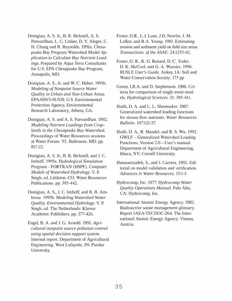
3 5

Donigian, A. S. Jr., B. R. Bicknell, A. S. Patwardhan, L. C. Linker, D. Y. Alegre, C. H. Chang and R. Reynolds. 1991a. Chesa-peake Bay Program Watershed Model Ap-plication to Calculate Bay Nutrient Load-ings. Prepared by Aqua Terra Consultants for U.S. EPA Chesapeake Bay Program, Annapolis, MD.

Donigian, A. S., Jr. and W. C. Huber. 1991b. Modeling of Nonpoint Source Water Quality in Urban and Non-Urban Areas. EPA/600/3-91/039. U.S. Environmental Protection Agency, Environmental Research Laboratory, Athens, GA.

Donigian, A. S. and A. S. Patwardhan. 1992. Modeling Nutrient Loadings from Crop-lands in the Chesapeake Bay Watershed. Proceedings of Water Resources sessions at Water Forum ’92. Baltimore, MD. pp. 817-22.

Donigian, A. S. Jr., B. R. Bicknell, and J. C. Imhoff. 1995a. Hydrological Simulation Program - FORTRAN (HSPF). Computer Models of Watershed Hydrology. V. P. Singh, ed. Littleton, CO: Water Resources Publications. pp. 395-442.

Donigian, A. S., J. C. Imhoff, and R. B. Am-brose. 1995b. Modeling Watershed Water Quality. Environmental Hydrology. V. P. Singh, ed. The Netherlands: Kluwer Academic Publishers. pp. 377-426.

Engel, B. A. and J. G. Arnold. 1991. Agri-cultural nonpoint source pollution control using spatial decision support system. Internal report. Department of Agricultural Engineering. West Lafayette, IN: Purdue University.

Foster, G.R., L.J. Lane, J.D. Nowlin, J. M. Laflen, and R.A. Young. 1981. Estimating erosion and sediment yield on field size areas. Transactions. of the ASAE. 24:1253-62.

Foster, G. R., K. G. Renard, D. C. Yoder, D. K. McCool, and G. A. Weesies. 1996. RUSLE User’s Guide. Ankey, IA: Soil and Water Conservation Society. 173 pp

Green, I.R.A. and D. Stephenson. 1986. Cri-teria for comparison of single event mod-els. Hydrological Sciences. 31: 395-411.

Haith, D. A. and L. L. Shoemaker. 1987. Generalized watershed loading functions for stream flow nutrients. Water Resources Bulletin. 107:121-37.

Haith, D. A., R. Mandel, and R. S. Wu. 1992. GWLF – Generalized Watershed Loading Functions, Version 2.0—User’s manual. Department of Agricultural Engineering, Ithaca, NY: Cornell University.

Hasssanizadeh, S., and J. Carrera. 1992. Edi-torial on model validation and verification. Advances in Water Resources. 15:1-3.

Hydrocomp, Inc. 1977. Hydrocomp Water Quality Operations Manual. Palo Alto, CA: Hydrocomp, Inc.

International Atomic Energy Agency. 1982. Radioactive waste management glossary. Report IAEA-TECDOC-264. The Inter-national Atomic Energy Agency. Vienna, Austria.

3 6

Johansen, R. C., J. C. Imhoff, J. L. Kittle, Jr. and A. S. Donigian. 1984. Hydrological Simulation Program—FORTRAN (HSPF): Users Manual for Release 8.0. EPA-600/3-84-066, Environmental Research Laboratory, U.S. Environmental Protection Agency, Athens, GA. 30613.

Knisel, W. G.1980. CREAMS: A Field-Scale Model for Chemicals, Runoff, and Erosion from Agricultural Management Systems. U.S. Department of Agriculture, Conserva-tion Research Report No. 26. U.S. Depart-ment of Agriculture, Washington, DC.

Leonard, R. A., W. G. Knisel, and D. A. Still. 1987. GLEAMS: Groundwater Loading Effects of Agricultural Management Sys-tems. Transactions of the ASAE. 30:1403-18.

Loague, K. and Green R.E. 1991. Statistical and graphical methods for evaluating solute transport models. Journal of Contaminate Hydrology. 7:51-73.

Lumb, A. M., J. L. Kittle, and K. M. Flynn. 1990. User’s manual for ANNIE, A com-puter program for interactive hydrologic analyses and data management. Water Resources Investigations Report 89-4080. Reston, VA: U.S. Geological Survey.

Lumb, A. M., and J. L. Kittle. 1993. Expert System for calibration and application of watershed models. Proceedings of the Fed-eral Interagency Workshop on Hydrologic Modeling Demands for the 90s. Water Resources Investigation Report 93-4018. Fort Collins, CO: U.S. Geological Survey.

Penman, H.L. 1948. Natural evaporation from open water, bare soil and grass. Proceedings of the Royal Society, London. A193: 120-146.

Manguerra, H. B. and B. A. Engel. 1998. Hydrologic parameterization of watershed for runoff prediction using SWAT. Journal of the American Water Resources Associa-tion. 34-5:1149-62.

McElroy, A. D., S. W. Chiu, J. W. Nabgen, A. Aleti, and R. W. Bennett. 1976. Loading functions for assessment of water pollution for non-point sources. EPA 600/2-76/151. U.S. Environmental Protection Agency, Washington, DC.

Mills, W. B. 1985. Water quality assessment: A screening procedure for toxic and con-ventional pollutants in surface and ground water. EPA/600/6-85/002a. Environmental Research Laboratory, U.S. Environmental Protection Agency, Athens, GA.

Moore, L. W., C. Y. Chew, R. H. Smith, and S. Sahoo. 1992. Modeling of best manage-ment practices on North Reelfoot Creek, Tennessee. Water Environment Research. 64:241-47.

Novotny, V. and H. Olem. 1994. Water Quality: Prevention, Identification, and Management of Diffuse Pollution. New York, NY: van Nostrand Reinhold.

Omnicron Associates. 1990. Nonpoint Pollution Source Model for Analysis and Planning—User’s Manual. Portland, OR: Omnicron Associates.

Preston, S. D. and J. W. Brakebill. 1999. Application of Spatially Referenced Re-gression Modeling for the Evaluation of Total Nitrogen Loading in the Chesapeake Bay Watershed. Water Resources Investiga-tions Report 99-4054. Baltimore, MD: U.S. Geological Survey.

3 7

Renard, K.G., G.R. Foster. G.A. Weesies, D. K. McCool. And D.C. Yoder. 1997. Pre-dicting Soil Erosion by Water: A Guide to Conservation Planning with the Revised Soil Loss Equation (RUSLE). Agricultural Handbook No. 703. Washington, DC: U.S. Government Printing Office.

Rosenthal, W. D., R. Srinivasan, and J. G. Ar-nold. 1995. Alternative river management using a linked GIS-hydrology model. Transactions of the ASAE. 38:783-90.

Singer, M. P., F. D. Arnold, R. H. Cole, J. G. Arnold, and J. R. Williams. 1988. Use of SWRRB computer model for the National Pollutant Discharge Inventory. W. L. Lyle and T. J. Hoban, eds. Proceeding of the Symposium on Coastal Water Resources. pp. 119-31.

Smith, R. A., G. E. Schwarz, and R. B. Alexan-der. December, 1997. Regional interpretation of water-quality monitoring data. Water Resources Research. 33(12):2781-98.

Srinivasan, R. and J. G. Arnold. 1994. Integrating a basin-scale water quality model with GIS. Water Resources Bulletin. 30:441-52.

Srinivasan, R., J. G. Arnold, R. S. Muttiah, and J. R. Williams. 1998. Large area hy-drologic modeling and assessment, Part I: model development. Journal of the American Water Resources Association. 34:73-89

Tim, U. S. 1996a. Emerging technologies for hydrologic and water quality modeling research. Transactions of the ASAE. 39:465-76.

Tim, U. S. 1996b. Coupling vadose zone models with GIS: emerging trends and potential bottlenecks. Journal of Environ-mental Quality. 25:535-44.

Whitmore, A.P. 1991. A method for assess-ing the goodness of computer simulation of soil processes. Journal of Soil Science 42:289-99.

Wigman, M. R. 1972. The fitting, calibration, and validation of simulation models. Simulation. 18:188-92

Williams, J. R. and H. D. Berndt, 1977. Sediment yield prediction based on watershed hydrology. Transactions of the ASAE. 20:1100-04.

Williams, J. R., Jones, C. A., Kiniry, J. R. and Spanel, D. A. 1989. The EPIC crop growth model. Transactions of the ASAE. 32:497-511.

Young, R.A., M.A. Otterby , and A. Roos. 1982. A technique for evaluation feedlot pollution potential. Journal of Soil and Water Conservation. 37: 21-23.

Young, R., C. A. Onstad, D. D. Bosch, and W. P. Anderson. 1987. AGNPS: Agricultur-al Non-Point Source Pollution Model: A watershed analysis tool. USDA, Agri-cultural Research Service. Conservation Research Report 35. 77 pp.