Embed Size (px)
Citation preview
MAYSAN UNIVERSITY CE 306 TRAFFIC ENGINEERING COLLEGE OF ENGINEERING THIRD YEAR CIVIL ENGINEERING DEPARTMENT Dr. RAID AL SHADIDI
YEAR 2015 -2016
MAYSAN UNIVERSITY
COLLEGE of ENGINEERING
CIVIL ENGINEERING DEPARTMENT
THIRD YEAR
TRAFFIC ENGINEERING
COURSE NUMBER CE 306
References:
Traffic and Highway Engineering, Fourth Edition, Nicholas J. Garber , Lester A.
Hoel, University of Virginia. Text Book.
AASHTO (American Association of State Highway and Transportation), A Policy Of
Geometric Design Of Highways And Streets, Washington D.C. 2001.
Fambro, D.B. Determination Of SSD, Transportation Research Board (TRB).
Washington D.C. 1997.
HWC (Highway Capacity Manual) , TRB, National Research Council NCR,
Washington D.C. 2000.
The (Traffic Engineering Handbook)
Webester, F. V. and B. M. Cobbe.
Traffic Signals, R.R. L. Road Research Laboratory 19 66, Highway Maintenance and
Operation.
Syllabus:
Vehicle Speed, Vehicle Highway Distributions, Traffic Volume, Fundamental Relationships
between Speed-Flow and density, Capacity and Level of Services of Two Lane Highways,
Intersection Design, Intersection Control, Car Parking, Road User Safety
Hint: Keep a diary of all trips you make for a period of three to five days. Record the purpose
of each trip, how you traveled, the approximate distance traveled, and the trip time. What
conclusions can you draw from the data?
MAYSAN UNIVERSITY CE 306 TRAFFIC ENGINEERING COLLEGE OF ENGINEERING THIRD YEAR CIVIL ENGINEERING DEPARTMENT Dr. RAID AL SHADIDI
YEAR 2015 - 2016
Pag
e2
What is Traffic Engineering?
Transportation engineering is the application of technology and scientific
principles to the planning, functional design, operation, and management of
facilities for any mode of transportation in order to provide for the safe, rapid,
comfortable, convenient, economical, and environmentally compatible
movement of people and goods.
Traffic engineering is “that branch of engineering which applies technology,
science, and human factors to the planning, design, operations and
management of roads, streets, bikeways, highways, their networks, terminals,
and abutting lands.”
Objective of traffic engineering is to provide for the safe, rapid, comfortable,
efficient, convenient, and environmentally compatible movement of people,
goods, and services.
The functional areas within traffic engineering are described as follows:
Traffic Operations is the science of analysis, review, and application of traffic
tools and data systems—including accident and surveillance records—as well
as volume and other data gathering techniques necessary for traffic planning.
It includes the knowledge of operational characteristics of persons and vehicles
to determine the need for traffic control devices, their relationship with other
traffic characteristics and the determination of safe transportation systems.
Traffic Design consists of the design of traffic control devices and roadway
operational design. Operational design concerns the visible features of a
roadway dealing with such roadway elements as cross sections, curvature,
sight distance, channelization, and clearances; and thus it depends directly on
the characteristics of traffic flow.
Traffic Planning includes the determination of personal and freight travel
patterns on the basis of engineering analysis of the traffic and demographic
characteristics of present, future, and potential land use plans. The
determination of these patterns assists in the second step of traffic planning:
formulation of recommendations for transportation systems and networks of
roadways.
MAYSAN UNIVERSITY CE 306 TRAFFIC ENGINEERING COLLEGE OF ENGINEERING THIRD YEAR CIVIL ENGINEERING DEPARTMENT Dr. RAID AL SHADIDI
YEAR 2015 - 2016
Pag
e3
Traffic Engineering Research includes the investigation of theoretical and
applied aspects of all areas of traffic engineering to develop new knowledge,
interpretations, and applications. Research areas include hypothetical testing;
development of traffic hardware; theory formulation; and methods of analysis,
synthesis, and evaluation of existing phenomena and knowledge.
The traffic engineering profession has been growing and expanding its
horizons for the past 70 years. As each decade brings a shift in professional
activities to respond to technological advancements, the engineering field
needs to address new areas. This publication covers activities that are probably
not covered in the above definitions. Accordingly, the definitions will change
over time as the profession meets the public’s need for transportation.
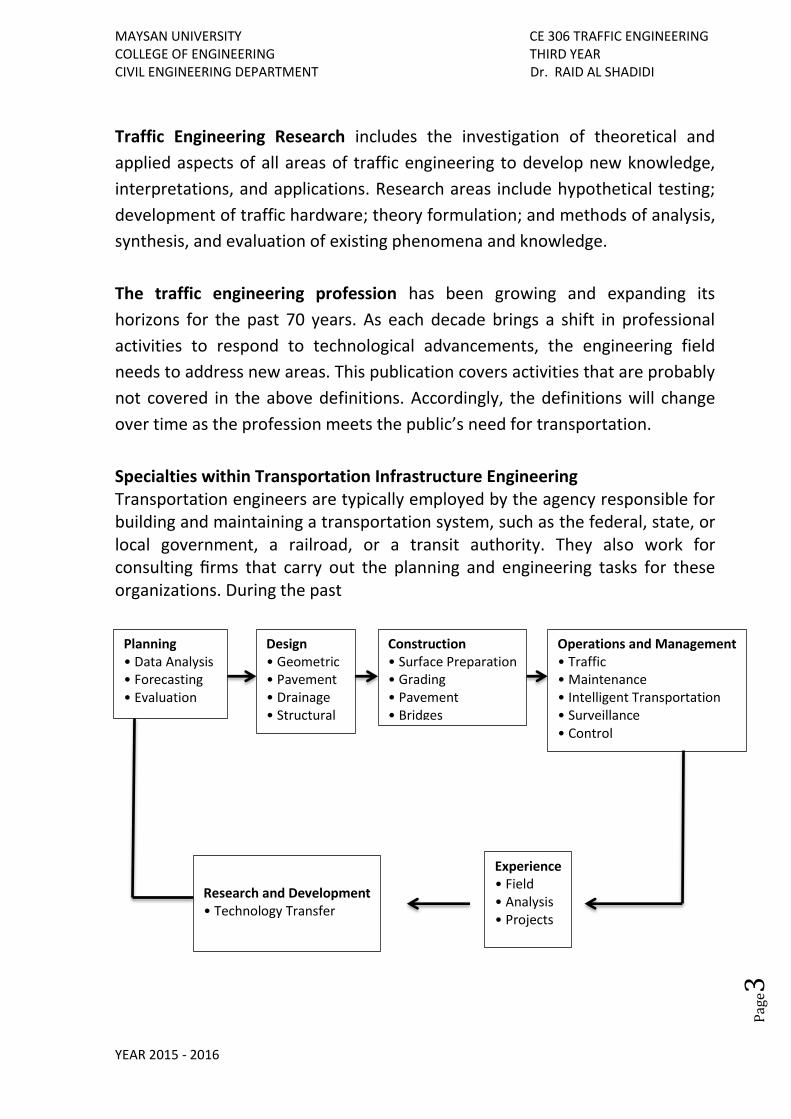
Specialties within Transportation Infrastructure Engineering Transportation engineers are typically employed by the agency responsible for building and maintaining a transportation system, such as the federal, state, or local government, a railroad, or a transit authority. They also work for consulting firms that carry out the planning and engineering tasks for these organizations. During the past
Planning • Data Analysis • Forecasting • Evaluation
Design • Geometric • Pavement • Drainage • Structural
Construction • Surface Preparation • Grading • Pavement • Bridges
Operations and Management • Traffic • Maintenance • Intelligent Transportation • Surveillance • Control
Experience • Field • Analysis • Projects
Research and Development • Technology Transfer
MAYSAN UNIVERSITY CE 306 TRAFFIC ENGINEERING COLLEGE OF ENGINEERING THIRD YEAR CIVIL ENGINEERING DEPARTMENT Dr. RAID AL SHADIDI
YEAR 2015 - 2016
Pag
e4
TRAFFIC OPERATIONS
The main components of the highway mode of transportation are;
Drivers
Pedestrians
Vehicles
Road
Bicycle is becoming an important component in the design of urban highways and streets.
Driver Characteristics:
1. Visual Reception:
a. Visual Acuity: ability to see fine details of the object.
Static Acuity, which is affected by background, brightness, contrast
and time, the optimal time required for identification of an object is
0.5 to 1.0 sec.
Dynamic Acuity: most people have clear vision within a conical angle
(3 – 5 degree), and fairly clear vision within a conical angle of (10 -12
degree).
The driver will clearly see those traffic devices that are within 12
degree cone, but objects outside this cone will be blurred.
b. Peripheral Vision: ability to see objects beyond the cone of the
clearest vision.
c. Color vision: ability to differentiate one color from another, color
blindness people see a combination of black and white or black and
yellow.
d. Glare vision and recovery
Direct: bright light appears in the individual’s field of vision.
Specular: when the image reflected by the bright light appears in the
field of vision.
Glare recovery: time required by a person to recover from the effect
of glare after passing the light source.
About 3 sec. when moving from dark ---- light.
About 6 sec. when moving from light -----dark.
e. Depth perception: ability to estimate speed and distance, especially
on two lane highway during passing maneuvers.
2. Hearing perception.
MAYSAN UNIVERSITY CE 306 TRAFFIC ENGINEERING COLLEGE OF ENGINEERING THIRD YEAR CIVIL ENGINEERING DEPARTMENT Dr. RAID AL SHADIDI
YEAR 2015 - 2016
Pag
e5
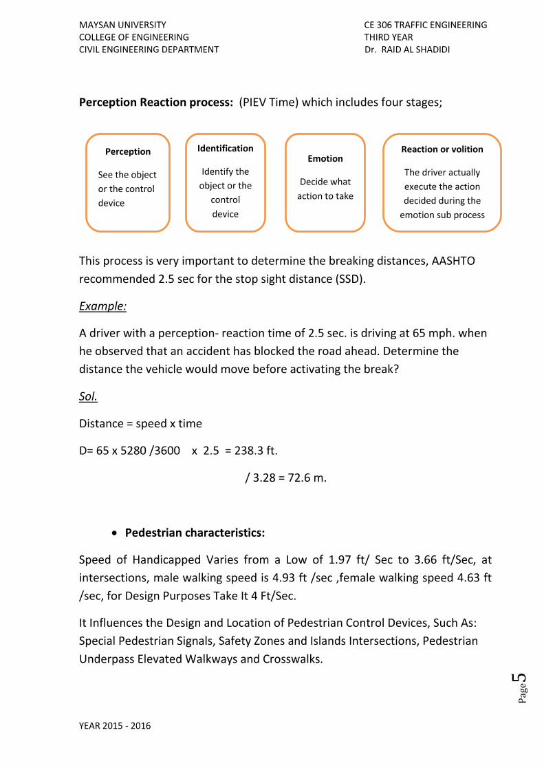
Perception Reaction process: (PIEV Time) which includes four stages;
This process is very important to determine the breaking distances, AASHTO
recommended 2.5 sec for the stop sight distance (SSD).
Example:
A driver with a perception- reaction time of 2.5 sec. is driving at 65 mph. when
he observed that an accident has blocked the road ahead. Determine the
distance the vehicle would move before activating the break?
Sol.
Distance = speed x time
D= 65 x 5280 /3600 x 2.5 = 238.3 ft.
/ 3.28 = 72.6 m.
Pedestrian characteristics:
Speed of Handicapped Varies from a Low of 1.97 ft/ Sec to 3.66 ft/Sec, at
intersections, male walking speed is 4.93 ft /sec ,female walking speed 4.63 ft
/sec, for Design Purposes Take It 4 Ft/Sec.
It Influences the Design and Location of Pedestrian Control Devices, Such As:
Special Pedestrian Signals, Safety Zones and Islands Intersections, Pedestrian
Underpass Elevated Walkways and Crosswalks.
Perception
See the object
or the control
device
Identification
Identify the
object or the
control
device
Emotion
Decide what
action to take
Reaction or volition
The driver actually
execute the action
decided during the
emotion sub process
MAYSAN UNIVERSITY CE 306 TRAFFIC ENGINEERING COLLEGE OF ENGINEERING THIRD YEAR CIVIL ENGINEERING DEPARTMENT Dr. RAID AL SHADIDI
YEAR 2015 - 2016
Pag
e6
Vehicle Characteristics:
Geometric design of highway depends on static, kinematic and dynamic
characteristics
Static characteristics:
Size of the design vehicle control the
Lane width
Shoulder width
Length and width of the parking bays
Length of the vertical curves
Axle weights
Pavement depths
Maximum grades
The maximum allowable truck sizes and weights are at most: • 80,000 lb gross weight, with axle loads of up to 20,000 lb for single axles and 34,000 lb for tandem (double) axles • 102 in. width for all trucks • 48 ft length for semitrailers and trailers • 28 ft length for each twin trailer
Estimating Allowable Gross Weight of a Truck
𝑊 = 500 ( 𝐿 𝑁
𝑁 − 1 + 12 𝑁 + 36 )
Where
𝑊 = overall gross weight (calculated to the nearest 500 lb)
𝐿 = the extreme of any group of two or more consecutive axles (ft)
𝑁 = number of axles in the group under consideration
MAYSAN UNIVERSITY CE 306 TRAFFIC ENGINEERING COLLEGE OF ENGINEERING THIRD YEAR CIVIL ENGINEERING DEPARTMENT Dr. RAID AL SHADIDI
YEAR 2015 - 2016
Pag
e7
Example: A 5-axle truck traveling on an interstate highway has the following axle characteristics: Distance between the front single axle and the first set of tandem axles _ 20 ft Distance between the first set of tandem axle and the back set of tandem axles _ 48 ft If the overall gross weight of the truck is 79,500 lb, determine whether this truck satisfies federal weight regulations. Sol: Although the overall gross weight is less than the maximum allowable of 80,000 lb, the allowable gross weight based on the axle configuration should be checked.
𝑊 = 500 ( 𝐿 𝑁
𝑁 − 1 + 12 𝑁 + 36 )
𝑊 = 500 ( 48 ∗ 4
4 − 1 + 12 ∗ 4 + 36 ) = 74000 𝑙𝑏
This is less than the allowable of 80,000 lb. The truck therefore satisfies the truck weight regulations. Kinematic characteristics: acceleration capability in passing, maneuvering and
gap acceptance.
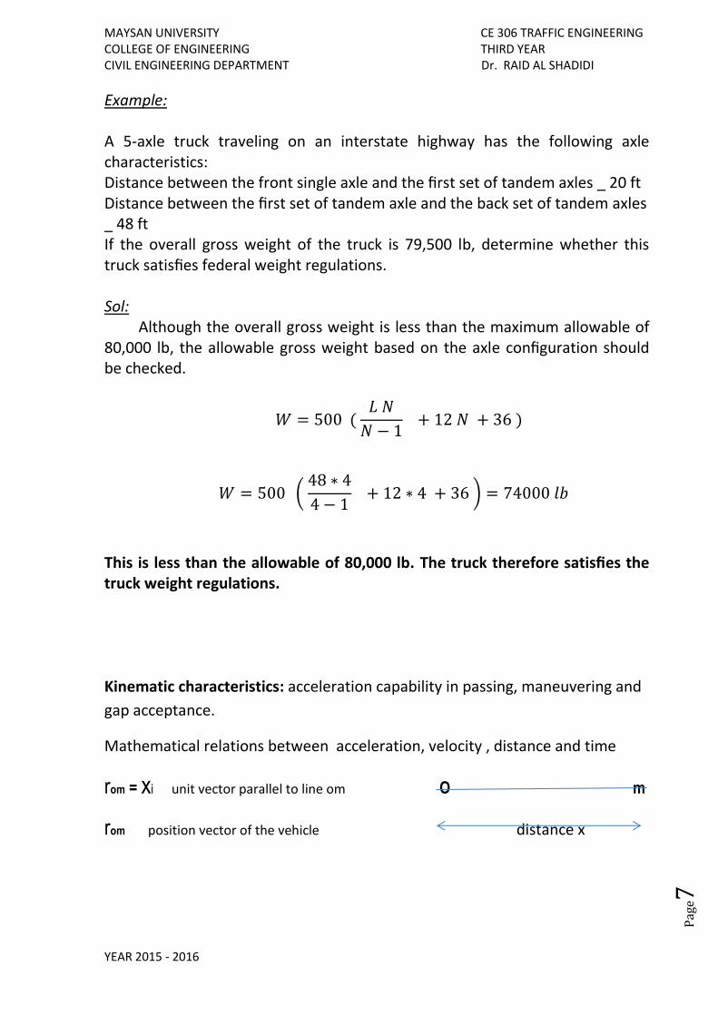
Mathematical relations between acceleration, velocity , distance and time
rom = xi unit vector parallel to line om O m
rom position vector of the vehicle distance x
MAYSAN UNIVERSITY CE 306 TRAFFIC ENGINEERING COLLEGE OF ENGINEERING THIRD YEAR CIVIL ENGINEERING DEPARTMENT Dr. RAID AL SHADIDI
YEAR 2015 - 2016
Pag
e8
Example:
Acceleration of a vehicle is represented by the equation;
𝑑𝑈𝑡
𝑑𝑡= 3.3 − 0.04 𝑈
Where (𝑈) = vehicle speed in ft/sec., if the vehicle is traveling at 45 mile/hr,
determine its velocity after 5 sec. of acceleration and distance traveled at that
time?
𝑈𝑡 =𝛼
𝛽 (1 − 𝑒−𝛽𝑡 ) + 𝑈 𝑒−𝛽𝑡
Where 𝛼 = 3.3 𝛽 = 0.04
Speed 𝑈 = 45 𝑚𝑖/ℎ = 66.15𝑓𝑡/𝑠𝑒𝑐.
𝑈𝑡 =3.3
0.04(1 − 𝑒−0.04∗5 ) + 66.15 ∗ 𝑒−0.04∗5
= 82.5 (1 − 0.82) + 66.15 ∗ 0.82 = 69.09𝑓𝑡
𝑠𝑒𝑐= 47
𝑚𝑖
ℎ
𝑋𝑡 =𝛼
𝛽 𝑡 −
𝛼
𝛽^2(1 − 𝑒−𝛽𝑡 ) +
𝑈
𝛽 (1 − 𝑒−𝛽𝑡)
=3.3
0.04∗ 5 −
3.3
0.04^2(1 − 𝑒−0.04∗5 ) +
66.15
0.04 (1 − 𝑒−0.04∗5)
= 338.93 𝑓𝑡
MAYSAN UNIVERSITY CE 306 TRAFFIC ENGINEERING COLLEGE OF ENGINEERING THIRD YEAR CIVIL ENGINEERING DEPARTMENT Dr. RAID AL SHADIDI
YEAR 2015 - 2016
Pag
e9
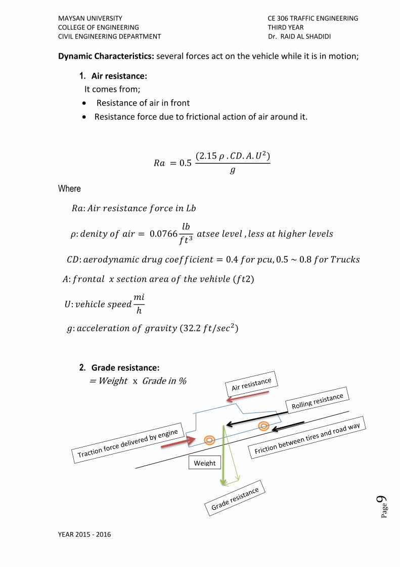
Dynamic Characteristics: several forces act on the vehicle while it is in motion;
1. Air resistance:
It comes from;
Resistance of air in front
Resistance force due to frictional action of air around it.
𝑅𝑎 = 0.5 (2.15 𝜌 . 𝐶𝐷. 𝐴. 𝑈2)
𝑔
Where
𝑅𝑎: 𝐴𝑖𝑟 𝑟𝑒𝑠𝑖𝑠𝑡𝑎𝑛𝑐𝑒 𝑓𝑜𝑟𝑐𝑒 𝑖𝑛 𝐿𝑏
𝜌: 𝑑𝑒𝑛𝑖𝑡𝑦 𝑜𝑓 𝑎𝑖𝑟 = 0.0766𝑙𝑏
𝑓𝑡3 𝑎𝑡𝑠𝑒𝑒 𝑙𝑒𝑣𝑒𝑙 , 𝑙𝑒𝑠𝑠 𝑎𝑡 ℎ𝑖𝑔ℎ𝑒𝑟 𝑙𝑒𝑣𝑒𝑙𝑠
𝐶𝐷: 𝑎𝑒𝑟𝑜𝑑𝑦𝑛𝑎𝑚𝑖𝑐 𝑑𝑟𝑢𝑔 𝑐𝑜𝑒𝑓𝑓𝑖𝑐𝑖𝑒𝑛𝑡 = 0.4 𝑓𝑜𝑟 𝑝𝑐𝑢, 0.5 ~ 0.8 𝑓𝑜𝑟 𝑇𝑟𝑢𝑐𝑘𝑠
𝐴: 𝑓𝑟𝑜𝑛𝑡𝑎𝑙 𝑥 𝑠𝑒𝑐𝑡𝑖𝑜𝑛 𝑎𝑟𝑒𝑎 𝑜𝑓 𝑡ℎ𝑒 𝑣𝑒ℎ𝑖𝑣𝑙𝑒 (𝑓𝑡2)
𝑈: 𝑣𝑒ℎ𝑖𝑐𝑙𝑒 𝑠𝑝𝑒𝑒𝑑𝑚𝑖
ℎ
𝑔: 𝑎𝑐𝑐𝑒𝑙𝑒𝑟𝑎𝑡𝑖𝑜𝑛 𝑜𝑓 𝑔𝑟𝑎𝑣𝑖𝑡𝑦 (32.2 𝑓𝑡/𝑠𝑒𝑐2)
2. Grade resistance:
= Weight x Grade in %
Weight
MAYSAN UNIVERSITY CE 306 TRAFFIC ENGINEERING COLLEGE OF ENGINEERING THIRD YEAR CIVIL ENGINEERING DEPARTMENT Dr. RAID AL SHADIDI
YEAR 2015 - 2016
Pag
e10
3. Rolling resistance:
Which depends on smoothness of pavement (lower on smooth
pavement than on rough pavement), and type of vehicle.
For (PCU) passenger car unit.
𝑅𝑟 = (𝐶𝑟𝑠 + 2.15𝐶𝑟𝑣 . 𝑈2)𝑊
Where
𝑅𝑟: 𝑟𝑜𝑙𝑙𝑖𝑛𝑔 𝑟𝑒𝑠𝑖𝑠𝑡𝑎𝑛𝑐𝑒 𝑓𝑜𝑟𝑐𝑒 (𝑙𝑏)
𝐶𝑟𝑠: 𝑐𝑜𝑛𝑠𝑡𝑎𝑛𝑡 (0.012)
𝐶𝑟𝑣: 𝑐𝑜𝑛𝑠𝑡𝑎𝑛𝑡 (0.65 ∗ 10−6 sec2/𝑓𝑡2
. 𝑈: 𝑣𝑒ℎ𝑖𝑐𝑙𝑒 𝑠𝑝𝑒𝑒𝑑 𝑚𝑖/ℎ
𝑊: 𝑔𝑟𝑜𝑠𝑠 𝑤𝑒𝑖𝑔ℎ𝑡 𝑜𝑓 𝑡ℎ𝑒 𝑣𝑒ℎ𝑖𝑐𝑙𝑒 (𝑙𝑏)
For Trucks
𝑅𝑟 = (𝐶𝑎 + 1.47𝐶𝑏 . 𝑈)𝑊
Where
𝐶𝑎 = 0.02445
𝐶𝑏 = 0.00044𝑠𝑒𝑐
𝑓𝑡
4. Curve resistance:
𝑅𝑐 = 0.5 (2.15 𝑈2𝑊)
𝑔. 𝑅
Where
𝑅𝑐: 𝐶𝑢𝑟𝑣𝑒 𝑟𝑒𝑠𝑖𝑠𝑡𝑎𝑛𝑐 (𝑙𝑏)
𝑈: 𝑣𝑒ℎ𝑖𝑐𝑙𝑒 𝑠𝑝𝑒𝑒𝑑 𝑚𝑖/ℎ
𝑅: 𝑅𝑎𝑑𝑢𝑖𝑠 𝑜𝑓 𝑐𝑢𝑟𝑣𝑎𝑡𝑢𝑟𝑒 (𝑓𝑡)
MAYSAN UNIVERSITY CE 306 TRAFFIC ENGINEERING COLLEGE OF ENGINEERING THIRD YEAR CIVIL ENGINEERING DEPARTMENT Dr. RAID AL SHADIDI
YEAR 2015 - 2016
Pag
e11
Power requirements
Vehicle horsepower is required to overcome resistance forces.
𝑃 = (1.47 𝑅 𝑈)
550
Where
𝑃 = ℎ𝑜𝑟𝑠𝑒𝑝𝑜𝑤𝑒𝑟 𝑑𝑒𝑙𝑖𝑣𝑒𝑟𝑒𝑑 (ℎ𝑝)
𝑅 = 𝑠𝑢𝑚 𝑜𝑓 𝑡ℎ𝑒 𝑟𝑒𝑠𝑖𝑠𝑡𝑎𝑛𝑐𝑒 𝑓𝑜𝑟𝑐𝑒𝑠 𝑡𝑜 𝑚𝑜𝑡𝑖𝑜𝑚 (𝑙𝑏)
𝑈 = 𝑠𝑝𝑒𝑒𝑑 𝑜𝑓 𝑣𝑒ℎ𝑖𝑐𝑙𝑒 (𝑚𝑖
ℎ)
Example:
Determine the horsepower produced by a PCU of 4000 lb. weight and 40 ft2
frontal sectional area, travelling at a speed 65 mi/h on a straight road of
smooth pavement and 5% grade?
Sol.
R=Air resistance + Rolling resistance + Grade resistance
𝑅 = 0.5 (2.15 ∗ 0.0766 ∗ 0.4 ∗ 40 ∗ 652)
32.2
+ (0.012 + 2.15 ∗ 0.65x10−6 ∗ 652) ∗ 4000 + 4000 ∗5
100= 444.5 𝑙𝑏.
𝑃 = (1.47 ∗ 444.5 ∗ 65)
550 = 77.2 ℎ𝑝
MAYSAN UNIVERSITY CE 306 TRAFFIC ENGINEERING COLLEGE OF ENGINEERING THIRD YEAR CIVIL ENGINEERING DEPARTMENT Dr. RAID AL SHADIDI
YEAR 2015 - 2016
Pag
e12
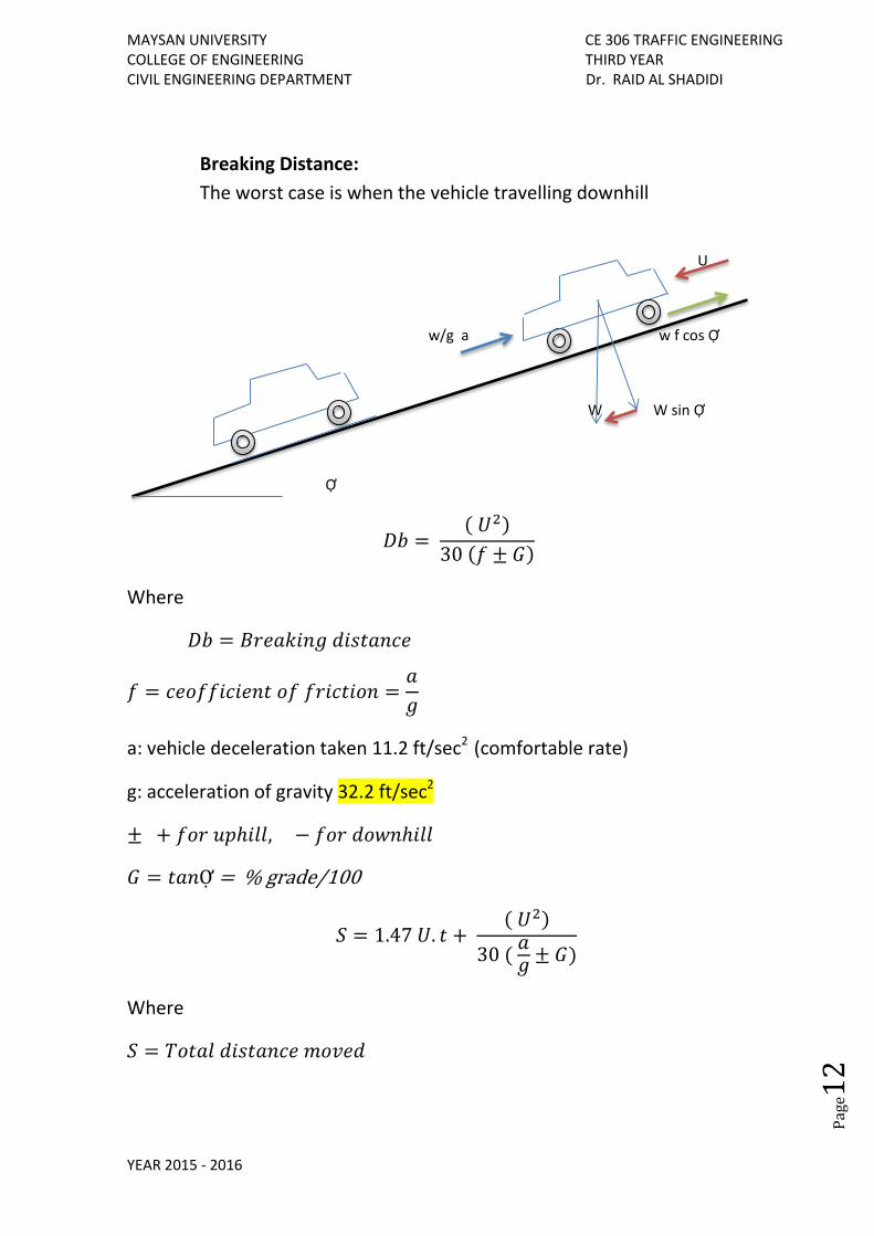
Breaking Distance:
The worst case is when the vehicle travelling downhill
U
w/g a w f cos Ợ
W W sin Ợ
Ợ
𝐷𝑏 = ( 𝑈2)
30 (𝑓 ± 𝐺)
Where
𝐷𝑏 = 𝐵𝑟𝑒𝑎𝑘𝑖𝑛𝑔 𝑑𝑖𝑠𝑡𝑎𝑛𝑐𝑒
𝑓 = 𝑐𝑒𝑜𝑓𝑓𝑖𝑐𝑖𝑒𝑛𝑡 𝑜𝑓 𝑓𝑟𝑖𝑐𝑡𝑖𝑜𝑛 =𝑎
𝑔
a: vehicle deceleration taken 11.2 ft/sec2 (comfortable rate)
g: acceleration of gravity 32.2 ft/sec2
± + 𝑓𝑜𝑟 𝑢𝑝ℎ𝑖𝑙𝑙, − 𝑓𝑜𝑟 𝑑𝑜𝑤𝑛ℎ𝑖𝑙𝑙
𝐺 = 𝑡𝑎𝑛Ợ = % grade/100
𝑆 = 1.47 𝑈. 𝑡 + ( 𝑈2)
30 ( 𝑎𝑔
± 𝐺)
Where
𝑆 = 𝑇𝑜𝑡𝑎𝑙 𝑑𝑖𝑠𝑡𝑎𝑛𝑐𝑒 𝑚𝑜𝑣𝑒𝑑
MAYSAN UNIVERSITY CE 306 TRAFFIC ENGINEERING COLLEGE OF ENGINEERING THIRD YEAR CIVIL ENGINEERING DEPARTMENT Dr. RAID AL SHADIDI
YEAR 2015 - 2016
Pag
e13
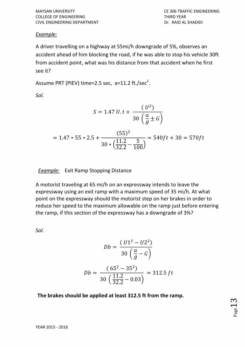
Example:
A driver travelling on a highway at 55mi/h downgrade of 5%, observes an
accident ahead of him blocking the road, if he was able to stop his vehicle 30ft
from accident point, what was his distance from that accident when he first
see it?
Assume PRT (PIEV) time=2.5 sec, a=11.2 ft./sec2.
Sol.
𝑆 = 1.47 𝑈. 𝑡 + ( 𝑈2)
30 ( 𝑎𝑔
± 𝐺)
= 1.47 ∗ 55 ∗ 2.5 +(55)2
30 ∗ (11.232.2
−5
100)= 540𝑓𝑡 + 30 = 570𝑓𝑡
Example: Exit Ramp Stopping Distance A motorist traveling at 65 mi/h on an expressway intends to leave the expressway using an exit ramp with a maximum speed of 35 mi/h. At what point on the expressway should the motorist step on her brakes in order to reduce her speed to the maximum allowable on the ramp just before entering the ramp, if this section of the expressway has a downgrade of 3%?
Sol.
𝐷𝑏 = ( 𝑈12 − 𝑈22)
30 ( 𝑎𝑔
− 𝐺)
𝐷𝑏 = ( 652 − 352)
30 ( 11.232.2
− 0.03) = 312.5 𝑓𝑡
The brakes should be applied at least 312.5 ft from the ramp.
MAYSAN UNIVERSITY CE 306 TRAFFIC ENGINEERING COLLEGE OF ENGINEERING THIRD YEAR CIVIL ENGINEERING DEPARTMENT Dr. RAID AL SHADIDI
YEAR 2015 - 2016
Pag
e14
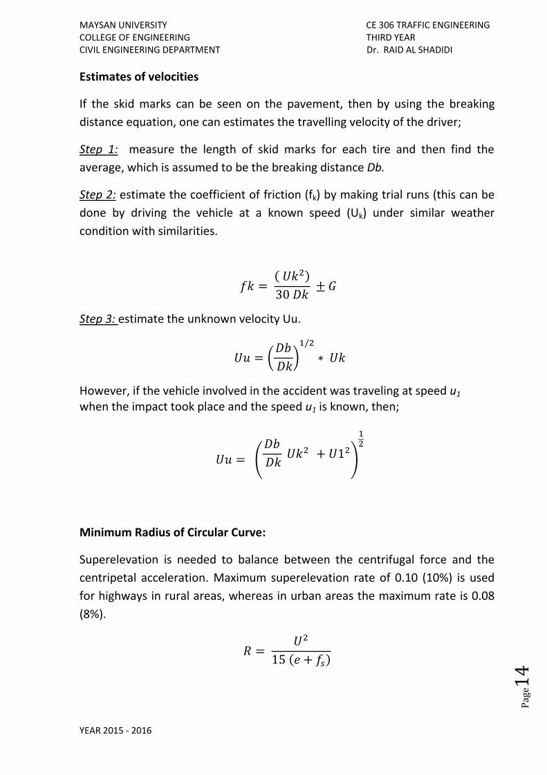
Estimates of velocities
If the skid marks can be seen on the pavement, then by using the breaking
distance equation, one can estimates the travelling velocity of the driver;
Step 1: measure the length of skid marks for each tire and then find the
average, which is assumed to be the breaking distance Db.
Step 2: estimate the coefficient of friction (fk) by making trial runs (this can be
done by driving the vehicle at a known speed (Uk) under similar weather
condition with similarities.
𝑓𝑘 = ( 𝑈𝑘2)
30 𝐷𝑘 ± 𝐺
Step 3: estimate the unknown velocity Uu.
𝑈𝑢 = (𝐷𝑏
𝐷𝑘)
1/2
∗ 𝑈𝑘
However, if the vehicle involved in the accident was traveling at speed u1 when the impact took place and the speed u1 is known, then;
𝑈𝑢 = (𝐷𝑏
𝐷𝑘 𝑈𝑘2 + 𝑈12
)
12
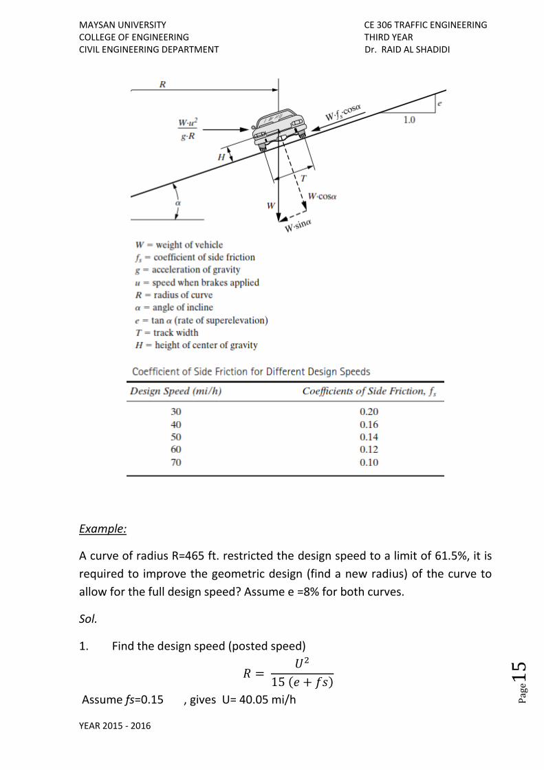
Minimum Radius of Circular Curve:
Superelevation is needed to balance between the centrifugal force and the
centripetal acceleration. Maximum superelevation rate of 0.10 (10%) is used
for highways in rural areas, whereas in urban areas the maximum rate is 0.08
(8%).
𝑅 = 𝑈2
15 (𝑒 + 𝑓𝑠)
MAYSAN UNIVERSITY CE 306 TRAFFIC ENGINEERING COLLEGE OF ENGINEERING THIRD YEAR CIVIL ENGINEERING DEPARTMENT Dr. RAID AL SHADIDI
YEAR 2015 - 2016
Pag
e15
Example:
A curve of radius R=465 ft. restricted the design speed to a limit of 61.5%, it is
required to improve the geometric design (find a new radius) of the curve to
allow for the full design speed? Assume e =8% for both curves.
Sol.
1. Find the design speed (posted speed)
𝑅 = 𝑈2
15 (𝑒 + 𝑓𝑠)
Assume fs=0.15 , gives U= 40.05 mi/h
MAYSAN UNIVERSITY CE 306 TRAFFIC ENGINEERING COLLEGE OF ENGINEERING THIRD YEAR CIVIL ENGINEERING DEPARTMENT Dr. RAID AL SHADIDI
YEAR 2015 - 2016
Pag
e16
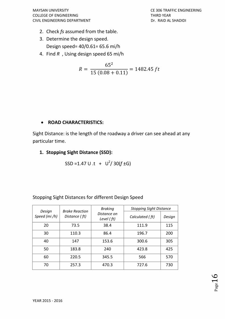
2. Check fs assumed from the table.
3. Determine the design speed.
Design speed= 40/0.61= 65.6 mi/h
4. Find R , Using design speed 65 mi/h
𝑅 = 652
15 (0.08 + 0.11)= 1482.45 𝑓𝑡
ROAD CHARACTERISTICS:
Sight Distance: is the length of the roadway a driver can see ahead at any
particular time.
1. Stopping Sight Distance (SSD):
SSD =1.47 U .t + U2/ 30(f ±G)
Stopping Sight Distances for different Design Speed
Design Speed (mi /h)
Brake Reaction Distance ( ft)
Braking Distance on
Level ( ft)
Stopping Sight Distance
Calculated ( ft) Design
20 73.5 38.4 111.9 115
30 110.3 86.4 196.7 200
40 147 153.6 300.6 305
50 183.8 240 423.8 425
60 220.5 345.5 566 570
70 257.3 470.3 727.6 730
MAYSAN UNIVERSITY CE 306 TRAFFIC ENGINEERING COLLEGE OF ENGINEERING THIRD YEAR CIVIL ENGINEERING DEPARTMENT Dr. RAID AL SHADIDI
YEAR 2015 - 2016
Pag
e17
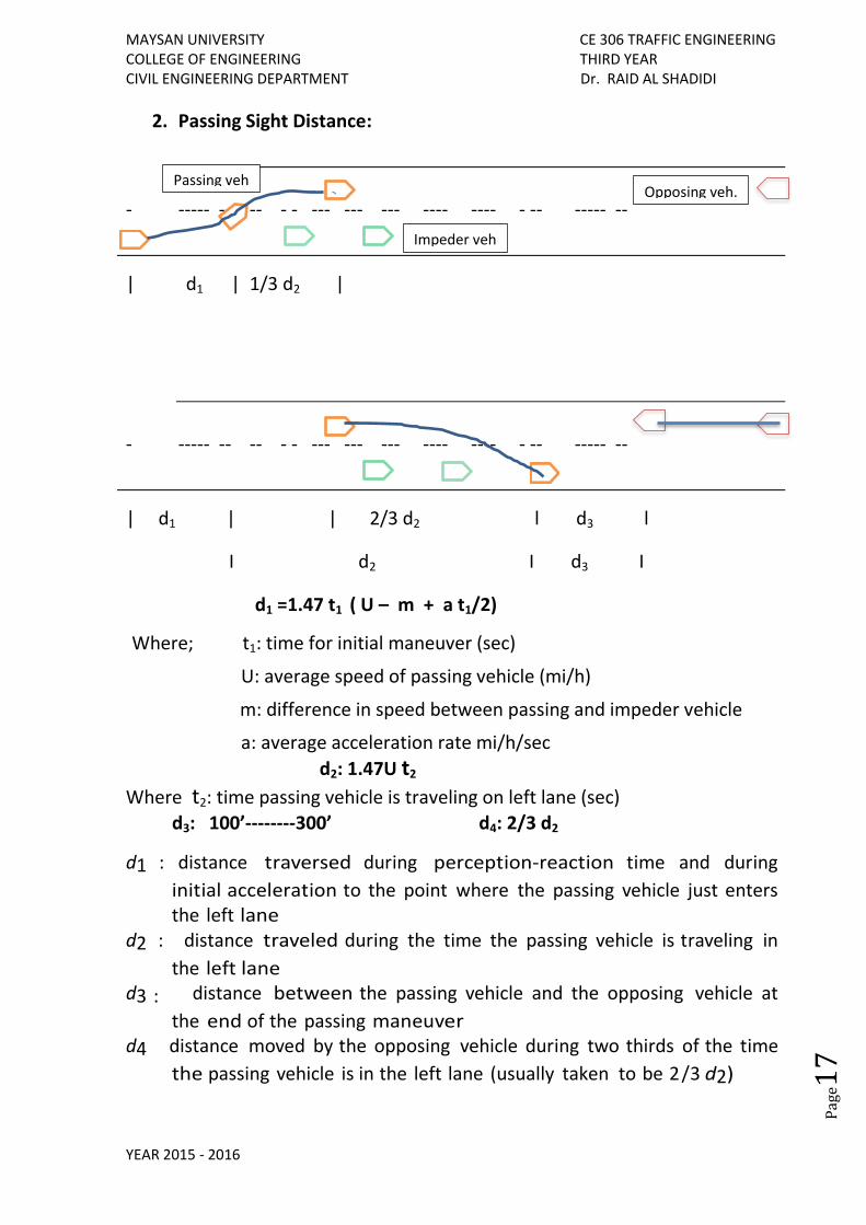
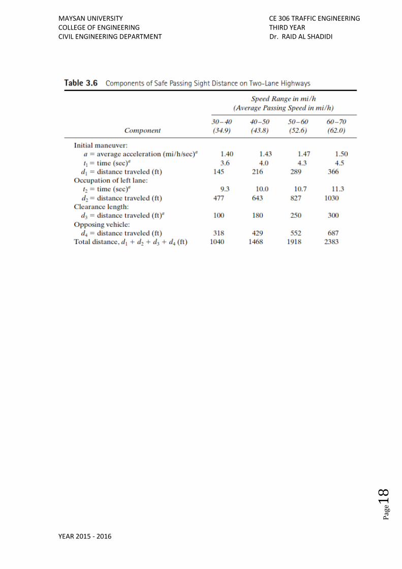
2. Passing Sight Distance:
- ----- -- -- - - --- --- --- ---- ---- - -- ----- --
| d1 | 1/3 d2 |
- ----- -- -- - - --- --- --- ---- ---- - -- ----- --
| d1 | | 2/3 d2 l d3 l
I d2 I d3 I
d1 =1.47 t1 ( U – m + a t1/2)
Where; t1: time for initial maneuver (sec)
U: average speed of passing vehicle (mi/h)
m: difference in speed between passing and impeder vehicle
a: average acceleration rate mi/h/sec
d2: 1.47U t2
Where t2: time passing vehicle is traveling on left lane (sec)
d3: 100’--------300’ d4: 2/3 d2
d1 : distance traversed during perception-reaction time and during
initial acceleration to the point where the passing vehicle just enters the left lane
d2 : distance traveled during the time the passing vehicle is traveling in
the left lane d3 : distance between the passing vehicle and the opposing vehicle at
the end of the passing maneuver d4 distance moved by the opposing vehicle during two thirds of the time
the passing vehicle is in the left lane (usually taken to be 2 /3 d2)
Opposing veh.
Impeder veh
Passing veh
MAYSAN UNIVERSITY CE 306 TRAFFIC ENGINEERING COLLEGE OF ENGINEERING THIRD YEAR CIVIL ENGINEERING DEPARTMENT Dr. RAID AL SHADIDI
YEAR 2015 - 2016
Pag
e18
MAYSAN UNIVERSITY CE 306 TRAFFIC ENGINEERING COLLEGE OF ENGINEERING THIRD YEAR CIVIL ENGINEERING DEPARTMENT Dr. RAID AL SHADIDI
YEAR 2015 - 2016
Pag
e19
TRAFFIC ENGINEERING STUDIES
Traffic studies may be grouped into three main categories:
(1) inventories, (2) administrative and (3) dynamic studies
Dynamic traffic studies involve the collection of data under operational
conditions and include studies of speed, traffic volume, travel time and delay,
parking, and crashes.
Spot Speed Studies
Duration of study is at least 1 hour and sample size at least 30 vehicle. It is
conducted to estimate the distribution of speed of vehicles in a stream of
traffic at a particular location on a highway. Speed characteristics identified by
such a study will be valid only for the traffic and environmental conditions that
exist at the time of the study and may be used to:
• Establish parameters for traffic operation and control, such as speed zones, speed limits (85th-percentile speed is commonly used as the speed limit on a road), and passing restrictions. • Evaluate the effectiveness of traffic control devices, such as variable message signs at work zones. • Monitor the effect of speed enforcement programs, such as the use of drone radar and the use of differential speed limits for passenger cars and trucks. • Evaluate and or determine the adequacy of highway geometric characteristics, such as radii of horizontal curves and lengths of vertical curves. • Evaluate the effect of speed on highway safety through the analysis of crash data for different speed characteristics. • Determine speed trends. • Determine whether complaints about speeding are valid. Methods for Conducting Spot Speed Studies 1. Road Detectors separated by a distance of 3 to 15 ft Road detectors can be classified into two general categories: pneumatic road tubes and induction loops. 2. Radar-Based Traffic Sensors 3. Electronic-Principle Detectors
MAYSAN UNIVERSITY CE 306 TRAFFIC ENGINEERING COLLEGE OF ENGINEERING THIRD YEAR CIVIL ENGINEERING DEPARTMENT Dr. RAID AL SHADIDI
YEAR 2015 - 2016
Pag
e20
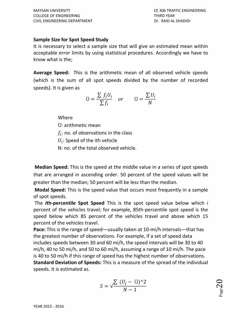
Sample Size for Spot Speed Study It is necessary to select a sample size that will give an estimated mean within acceptable error limits by using statistical procedures. Accordingly we have to know what is the; Average Speed: This is the arithmetic mean of all observed vehicle speeds
(which is the sum of all spot speeds divided by the number of recorded
speeds). It is given as
⩂ = ∑ 𝑓𝑖𝑈𝑖
∑ 𝑓𝑖 𝑜𝑟 ⩂ =
∑ 𝑈𝑖
𝑁
Where
⩂: arithmetic mean
𝑓𝑖: no. of observations in the class
𝑈𝑖: Speed of the ith vehicle
N: no. of the total observed vehicle.
Median Speed: This is the speed at the middle value in a series of spot speeds
that are arranged in ascending order. 50 percent of the speed values will be
greater than the median; 50 percent will be less than the median.
Modal Speed: This is the speed value that occurs most frequently in a sample of spot speeds. The ith-percentile Spot Speed This is the spot speed value below which i percent of the vehicles travel; for example, 85th-percentile spot speed is the speed below which 85 percent of the vehicles travel and above which 15 percent of the vehicles travel. Pace: This is the range of speed—usually taken at 10-mi/h intervals—that has the greatest number of observations. For example, if a set of speed data includes speeds between 30 and 60 mi/h, the speed intervals will be 30 to 40 mi/h, 40 to 50 mi/h, and 50 to 60 mi/h, assuming a range of 10 mi/h. The pace is 40 to 50 mi/h if this range of speed has the highest number of observations. Standard Deviation of Speeds: This is a measure of the spread of the individual speeds. It is estimated as.
𝑆 = √∑ (𝑈𝑗 − ⩂)^2
𝑁 − 1
MAYSAN UNIVERSITY CE 306 TRAFFIC ENGINEERING COLLEGE OF ENGINEERING THIRD YEAR CIVIL ENGINEERING DEPARTMENT Dr. RAID AL SHADIDI
YEAR 2015 - 2016
Pag
e21
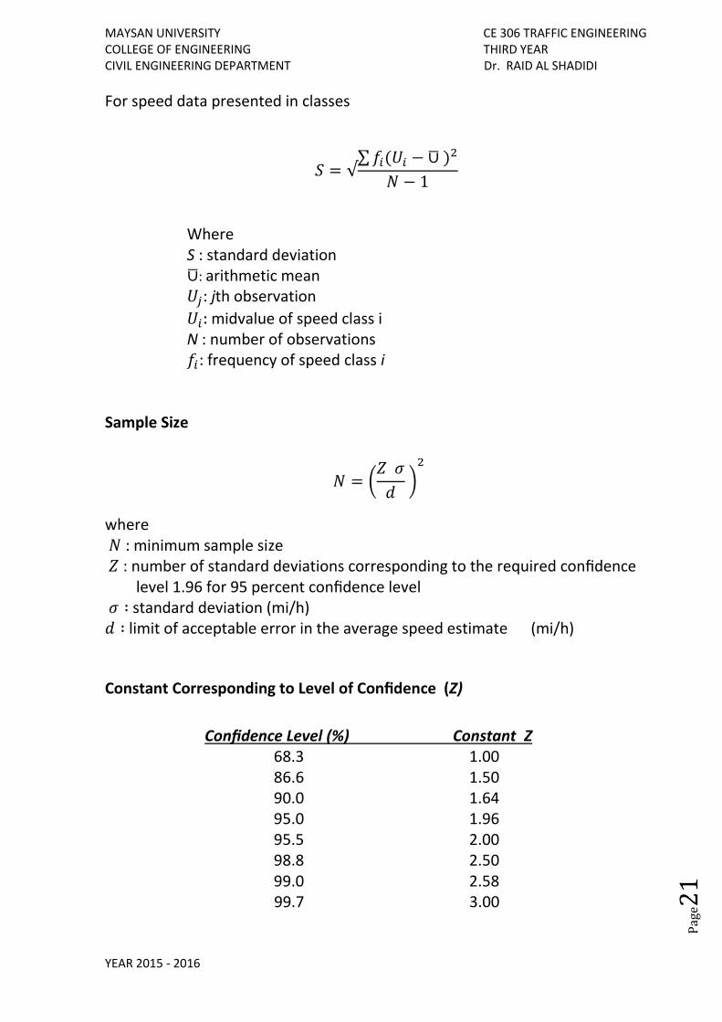
For speed data presented in classes
𝑆 = √∑ 𝑓𝑖(𝑈𝑖 − ⩂ )2
𝑁 − 1
Where S : standard deviation ⩂: arithmetic mean 𝑈𝑗: jth observation
𝑈𝑖: midvalue of speed class i N : number of observations 𝑓𝑖: frequency of speed class i
Sample Size
𝑁 = (𝑍 𝜎
𝑑 )
2
where 𝑁 : minimum sample size 𝑍 : number of standard deviations corresponding to the required confidence
level 1.96 for 95 percent confidence level 𝜎 ∶ standard deviation (mi/h) 𝑑 ∶ limit of acceptable error in the average speed estimate (mi/h)
Constant Corresponding to Level of Confidence (Z)
Confidence Level (%) Constant Z 68.3 1.00 86.6 1.50 90.0 1.64 95.0 1.96 95.5 2.00 98.8 2.50 99.0 2.58 99.7 3.00
MAYSAN UNIVERSITY CE 306 TRAFFIC ENGINEERING COLLEGE OF ENGINEERING THIRD YEAR CIVIL ENGINEERING DEPARTMENT Dr. RAID AL SHADIDI
YEAR 2015 - 2016
Pag
e22
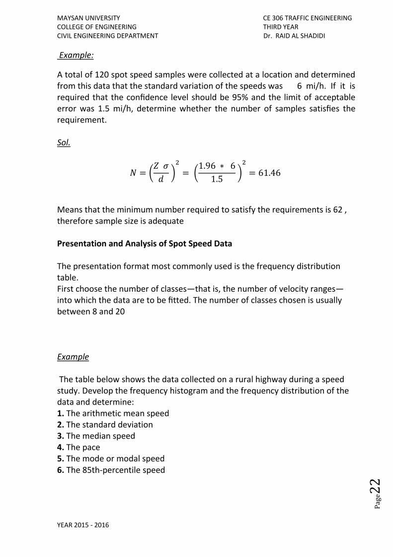
Example:
A total of 120 spot speed samples were collected at a location and determined from this data that the standard variation of the speeds was 6 mi/h. If it is required that the confidence level should be 95% and the limit of acceptable error was 1.5 mi/h, determine whether the number of samples satisfies the requirement. Sol.
𝑁 = (𝑍 𝜎
𝑑 )
2
= (1.96 ∗ 6
1.5 )
2
= 61.46
Means that the minimum number required to satisfy the requirements is 62 , therefore sample size is adequate Presentation and Analysis of Spot Speed Data The presentation format most commonly used is the frequency distribution table. First choose the number of classes—that is, the number of velocity ranges—into which the data are to be fitted. The number of classes chosen is usually between 8 and 20 Example The table below shows the data collected on a rural highway during a speed study. Develop the frequency histogram and the frequency distribution of the data and determine: 1. The arithmetic mean speed 2. The standard deviation 3. The median speed 4. The pace 5. The mode or modal speed 6. The 85th-percentile speed
MAYSAN UNIVERSITY CE 306 TRAFFIC ENGINEERING COLLEGE OF ENGINEERING THIRD YEAR CIVIL ENGINEERING DEPARTMENT Dr. RAID AL SHADIDI
YEAR 2015 - 2016
Pag
e23
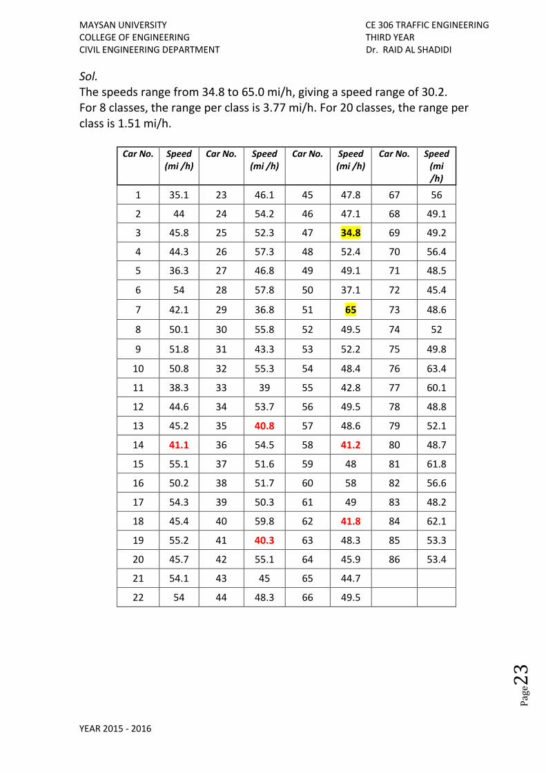
Sol. The speeds range from 34.8 to 65.0 mi/h, giving a speed range of 30.2. For 8 classes, the range per class is 3.77 mi/h. For 20 classes, the range per class is 1.51 mi/h.
Car No. Speed (mi /h)
Car No. Speed (mi /h)
Car No. Speed (mi /h)
Car No. Speed (mi /h)
1 35.1 23 46.1 45 47.8 67 56
2 44 24 54.2 46 47.1 68 49.1
3 45.8 25 52.3 47 34.8 69 49.2
4 44.3 26 57.3 48 52.4 70 56.4
5 36.3 27 46.8 49 49.1 71 48.5
6 54 28 57.8 50 37.1 72 45.4
7 42.1 29 36.8 51 65 73 48.6
8 50.1 30 55.8 52 49.5 74 52
9 51.8 31 43.3 53 52.2 75 49.8
10 50.8 32 55.3 54 48.4 76 63.4
11 38.3 33 39 55 42.8 77 60.1
12 44.6 34 53.7 56 49.5 78 48.8
13 45.2 35 40.8 57 48.6 79 52.1
14 41.1 36 54.5 58 41.2 80 48.7
15 55.1 37 51.6 59 48 81 61.8
16 50.2 38 51.7 60 58 82 56.6
17 54.3 39 50.3 61 49 83 48.2
18 45.4 40 59.8 62 41.8 84 62.1
19 55.2 41 40.3 63 48.3 85 53.3
20 45.7 42 55.1 64 45.9 86 53.4
21 54.1 43 45 65 44.7
22 54 44 48.3 66 49.5
MAYSAN UNIVERSITY CE 306 TRAFFIC ENGINEERING COLLEGE OF ENGINEERING THIRD YEAR CIVIL ENGINEERING DEPARTMENT Dr. RAID AL SHADIDI
YEAR 2015 - 2016
Pag
e24
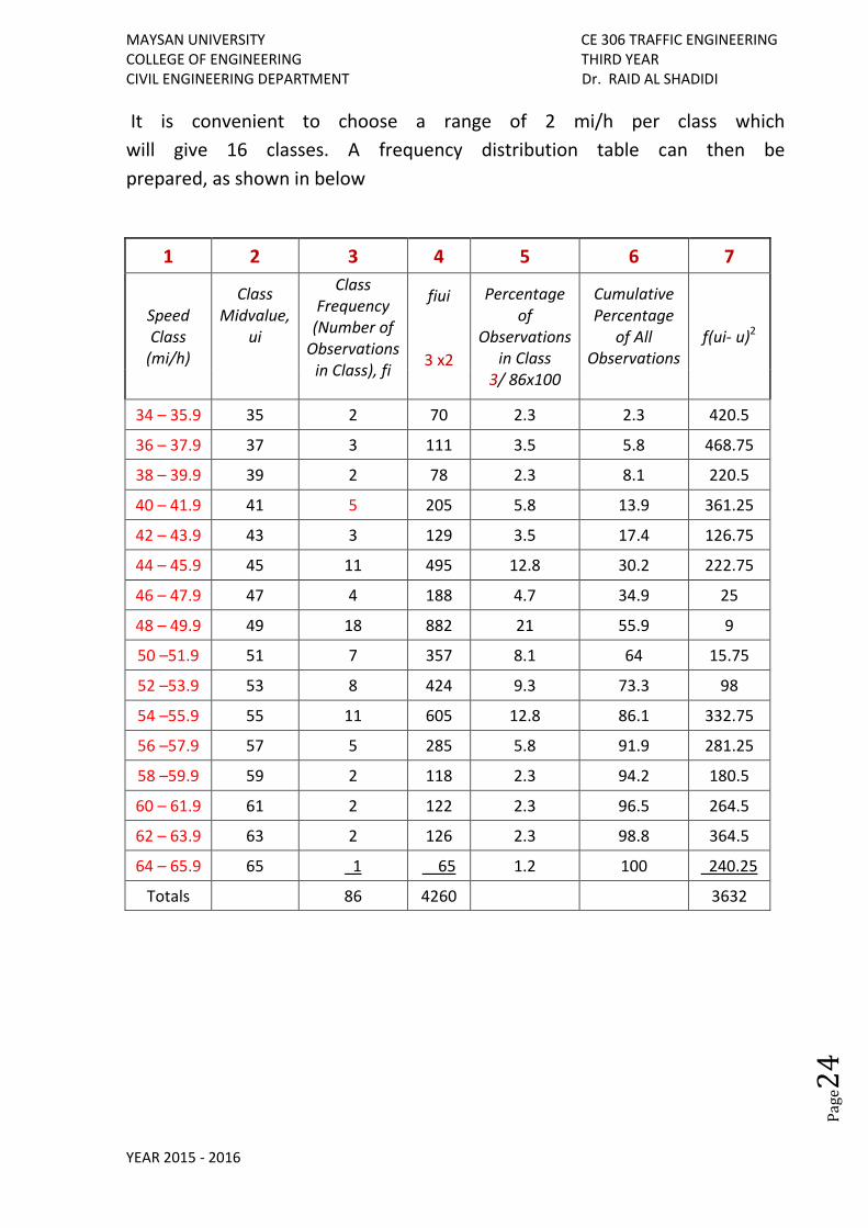
It is convenient to choose a range of 2 mi/h per class which
will give 16 classes. A frequency distribution table can then be
prepared, as shown in below
1 2 3 4 5 6 7
Speed Class
(mi/h)
Class Midvalue,
ui
Class Frequency
(Number of Observations
in Class), fi
fiui
3 x2
Percentage of
Observations in Class
3/ 86x100
Cumulative Percentage
of All Observations
f(ui- u)2
34 – 35.9 35 2 70 2.3 2.3 420.5
36 – 37.9 37 3 111 3.5 5.8 468.75
38 – 39.9 39 2 78 2.3 8.1 220.5
40 – 41.9 41 5 205 5.8 13.9 361.25
42 – 43.9 43 3 129 3.5 17.4 126.75
44 – 45.9 45 11 495 12.8 30.2 222.75
46 – 47.9 47 4 188 4.7 34.9 25
48 – 49.9 49 18 882 21 55.9 9
50 –51.9 51 7 357 8.1 64 15.75
52 –53.9 53 8 424 9.3 73.3 98
54 –55.9 55 11 605 12.8 86.1 332.75
56 –57.9 57 5 285 5.8 91.9 281.25
58 –59.9 59 2 118 2.3 94.2 180.5
60 – 61.9 61 2 122 2.3 96.5 264.5
62 – 63.9 63 2 126 2.3 98.8 364.5
64 – 65.9 65 1 65 1.2 100 240.25
Totals 86 4260 3632
MAYSAN UNIVERSITY CE 306 TRAFFIC ENGINEERING COLLEGE OF ENGINEERING THIRD YEAR CIVIL ENGINEERING DEPARTMENT Dr. RAID AL SHADIDI
YEAR 2015 - 2016
Pag
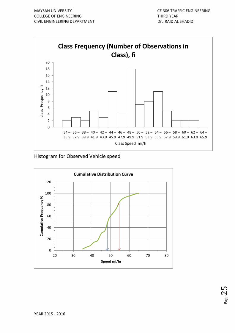
e25
Histogram for Observed Vehicle speed
0
2
4
6
8
10
12
14
16
18
20
34 – 35.9
36 – 37.9
38 – 39.9
40 – 41.9
42 – 43.9
44 – 45.9
46 – 47.9
48 – 49.9
50 –51.9
52 –53.9
54 –55.9
56 –57.9
58 –59.9
60 – 61.9
62 – 63.9
64 – 65.9
clas
s F
req
uen
cy f
i
Class Speed mi/h
Class Frequency (Number of Observations in Class), fi
0
20
40
60
80
100
120
20 30 40 50 60 70 80
Cu
mu
lati
ve F
req
uan
cy %
Speed mi/hr
Cumulative Distribution Curve
MAYSAN UNIVERSITY CE 306 TRAFFIC ENGINEERING COLLEGE OF ENGINEERING THIRD YEAR CIVIL ENGINEERING DEPARTMENT Dr. RAID AL SHADIDI
YEAR 2015 - 2016
Pag
e26
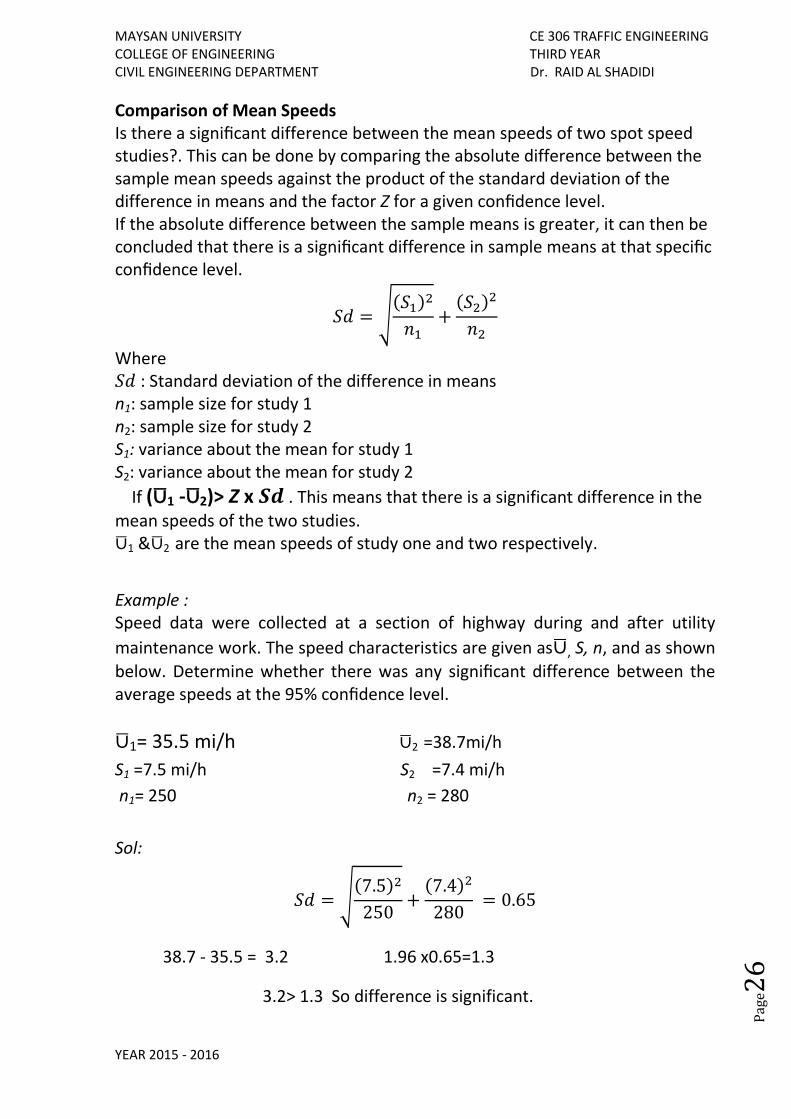
Comparison of Mean Speeds Is there a significant difference between the mean speeds of two spot speed studies?. This can be done by comparing the absolute difference between the sample mean speeds against the product of the standard deviation of the difference in means and the factor Z for a given confidence level. If the absolute difference between the sample means is greater, it can then be concluded that there is a significant difference in sample means at that specific confidence level.
𝑆𝑑 = √(𝑆1)2
𝑛1+
(𝑆2)2
𝑛2
Where 𝑆𝑑 : Standard deviation of the difference in means n1: sample size for study 1 n2: sample size for study 2 S1: variance about the mean for study 1 S2: variance about the mean for study 2
If (⩂1 -⩂2)˃ Z x 𝑺𝒅 . This means that there is a significant difference in the
mean speeds of the two studies. ⩂1 &⩂2 are the mean speeds of study one and two respectively.
Example : Speed data were collected at a section of highway during and after utility
maintenance work. The speed characteristics are given as⩂, S, n, and as shown
below. Determine whether there was any significant difference between the average speeds at the 95% confidence level.
⩂1= 35.5 mi/h ⩂2 =38.7mi/h
S1 =7.5 mi/h S2 =7.4 mi/h
n1= 250 n2 = 280
Sol:
𝑆𝑑 = √(7.5)2
250+
(7.4)2
280 = 0.65
38.7 - 35.5 = 3.2 1.96 x0.65=1.3
3.2˃ 1.3 So difference is significant.
MAYSAN UNIVERSITY CE 306 TRAFFIC ENGINEERING COLLEGE OF ENGINEERING THIRD YEAR CIVIL ENGINEERING DEPARTMENT Dr. RAID AL SHADIDI
YEAR 2015 - 2016
Pag
e27
Traffic Volume
Is the number of vehicles and/or pedestrians that pass a point on a highway facility during a specified time period. This time period varies from as little as 15 minutes to as much as a year depending on the anticipated use of the data. The data collected also may be put into subclasses which may include directional movement, occupancy rates, vehicle classification, and pedestrian age. Traffic volume studies are usually conducted when certain volume characteristics are needed, some of which follow: 1. Average Annual Daily Traffic (AADT) is the average of 24-hour counts
collected every day of the year
AADT=𝑎𝑣𝑒𝑟𝑎𝑔𝑒 24 ℎ 𝑣𝑜𝑙.𝑓𝑜𝑟 𝑒𝑎𝑐ℎ 𝑑𝑎𝑦(𝑛𝑜.𝑜𝑓 𝑣𝑒ℎ𝑖𝑐𝑙𝑒𝑠)
365 𝑑𝑎𝑦𝑠 𝑜𝑟 366 𝑓𝑜𝑟 𝑙𝑒𝑎𝑝 𝑦𝑒𝑎𝑟
AADTs are used in several traffic and transportation analyses for: a. Estimation of highway user revenues b. Computation of crash rates in terms of number of crashes per 100 million vehicle miles. c. Establishment of traffic volume trends d. Evaluation of the economic feasibility of highway projects e. Development of freeway and major arterial street systems f. Development of improvement and maintenance programs 2.Average annual weekday traffic
AAWT= 𝑎𝑣𝑒𝑟𝑎𝑔𝑒 24 ℎ 𝑣𝑜𝑙.𝑓𝑜𝑟 𝑒𝑎𝑐ℎ 𝑑𝑎𝑦(𝑛𝑜.𝑜𝑓 𝑣𝑒ℎ𝑖𝑐𝑙𝑒𝑠)
𝑛𝑜.𝑜𝑓 𝑤𝑒𝑒𝑘𝑑𝑎𝑦𝑠 (260 𝑢𝑠𝑢𝑎𝑙𝑙𝑦)
3. Average Daily Traffic (ADT) is the average of 24-hour counts collected over a number of days greater than one but less than a year. ADTs may be used for: a. Planning of highway activities b. Measurement of current demand c. Evaluation of existing traffic flow 4. Peak Hour Volume (PHV) is the maximum number of vehicles that pass a point on a highway during a period of 60 consecutive minutes. PHVs are used for: a. Functional classification of highways b. Design of the geometric characteristics of a highway, for example, number of lanes, intersection signalization, or channelization c. Capacity analysis d. Development of programs related to traffic operations, for example, one-way street systems or traffic routing e. Development of parking regulations
MAYSAN UNIVERSITY CE 306 TRAFFIC ENGINEERING COLLEGE OF ENGINEERING THIRD YEAR CIVIL ENGINEERING DEPARTMENT Dr. RAID AL SHADIDI
YEAR 2015 - 2016
Pag
e28
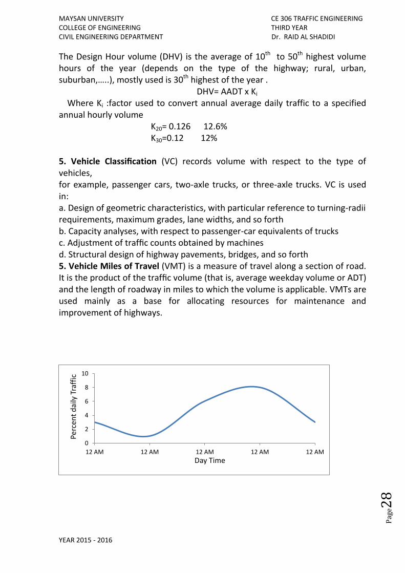
The Design Hour volume (DHV) is the average of 10th to 50th highest volume hours of the year (depends on the type of the highway; rural, urban, suburban,…..), mostly used is 30th highest of the year . DHV= AADT x Ki
Where Ki :factor used to convert annual average daily traffic to a specified annual hourly volume K20= 0.126 12.6% K30=0.12 12% 5. Vehicle Classification (VC) records volume with respect to the type of vehicles, for example, passenger cars, two-axle trucks, or three-axle trucks. VC is used in: a. Design of geometric characteristics, with particular reference to turning-radii requirements, maximum grades, lane widths, and so forth b. Capacity analyses, with respect to passenger-car equivalents of trucks c. Adjustment of traffic counts obtained by machines d. Structural design of highway pavements, bridges, and so forth 5. Vehicle Miles of Travel (VMT) is a measure of travel along a section of road. It is the product of the traffic volume (that is, average weekday volume or ADT) and the length of roadway in miles to which the volume is applicable. VMTs are used mainly as a base for allocating resources for maintenance and improvement of highways.
0
2
4
6
8
10
12 AM 12 AM 12 AM 12 AM 12 AM
Perc
ent
dai
ly T
raff
ic
Day Time
MAYSAN UNIVERSITY CE 306 TRAFFIC ENGINEERING COLLEGE OF ENGINEERING THIRD YEAR CIVIL ENGINEERING DEPARTMENT Dr. RAID AL SHADIDI
YEAR 2015 - 2016
Pag
e29
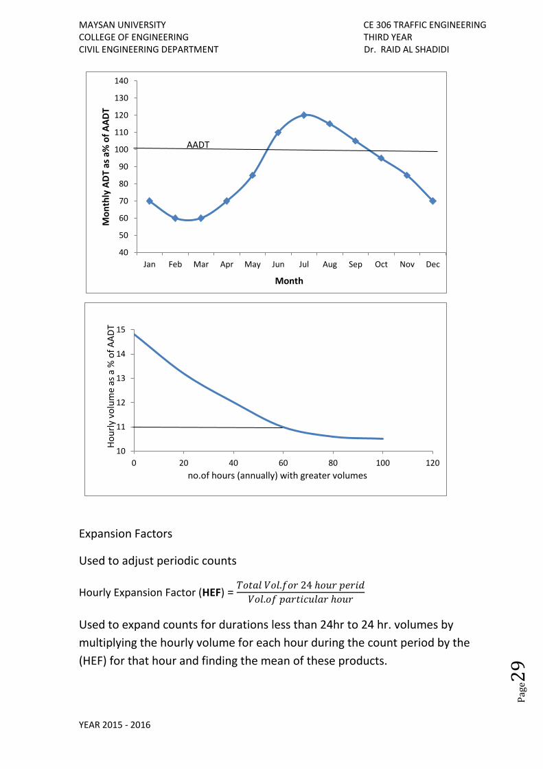
Expansion Factors
Used to adjust periodic counts
Hourly Expansion Factor (HEF) = 𝑇𝑜𝑡𝑎𝑙 𝑉𝑜𝑙.𝑓𝑜𝑟 24 ℎ𝑜𝑢𝑟 𝑝𝑒𝑟𝑖𝑑
𝑉𝑜𝑙.𝑜𝑓 𝑝𝑎𝑟𝑡𝑖𝑐𝑢𝑙𝑎𝑟 ℎ𝑜𝑢𝑟
Used to expand counts for durations less than 24hr to 24 hr. volumes by
multiplying the hourly volume for each hour during the count period by the
(HEF) for that hour and finding the mean of these products.
40
50
60
70
80
90
100
110
120
130
140
Jan Feb Mar Apr May Jun Jul Aug Sep Oct Nov Dec
Mo
nth
ly A
DT
as a
% o
f A
AD
T
Month
AADT
10
11
12
13
14
15
0 20 40 60 80 100 120
Ho
url
y vo
lum
e as
a %
of
AA
DT
no.of hours (annually) with greater volumes
MAYSAN UNIVERSITY CE 306 TRAFFIC ENGINEERING COLLEGE OF ENGINEERING THIRD YEAR CIVIL ENGINEERING DEPARTMENT Dr. RAID AL SHADIDI
YEAR 2015 - 2016
Pag
e30
Daily Expansion Factor (DEF) = 𝐴𝑣𝑒𝑟𝑎𝑔𝑒 𝑡𝑜𝑡𝑎𝑙 𝑣𝑜𝑙𝑢𝑚𝑒 𝑓𝑜𝑟 𝑤𝑒𝑒𝑘
𝐴𝑣𝑒𝑟𝑎𝑔𝑒 𝑣𝑜𝑙. 𝑝𝑎𝑟𝑡𝑖𝑐𝑢𝑙𝑎𝑟 𝑑𝑎𝑦
Used to determine weekly volumes from counts of 24hr duration by multiplying the 24 hr. volume by the DEF.
Monthly Expansion Factor (MEF) = 𝐴𝐴𝐷𝑇
𝐴𝐷𝑇 𝑓𝑜𝑟 𝑝𝑎𝑟𝑡𝑖𝑐𝑢𝑙𝑎𝑟 𝑚𝑜𝑛𝑡ℎ
Used to determine the AADT by multiplying the ADT for a given month by the
MEF.
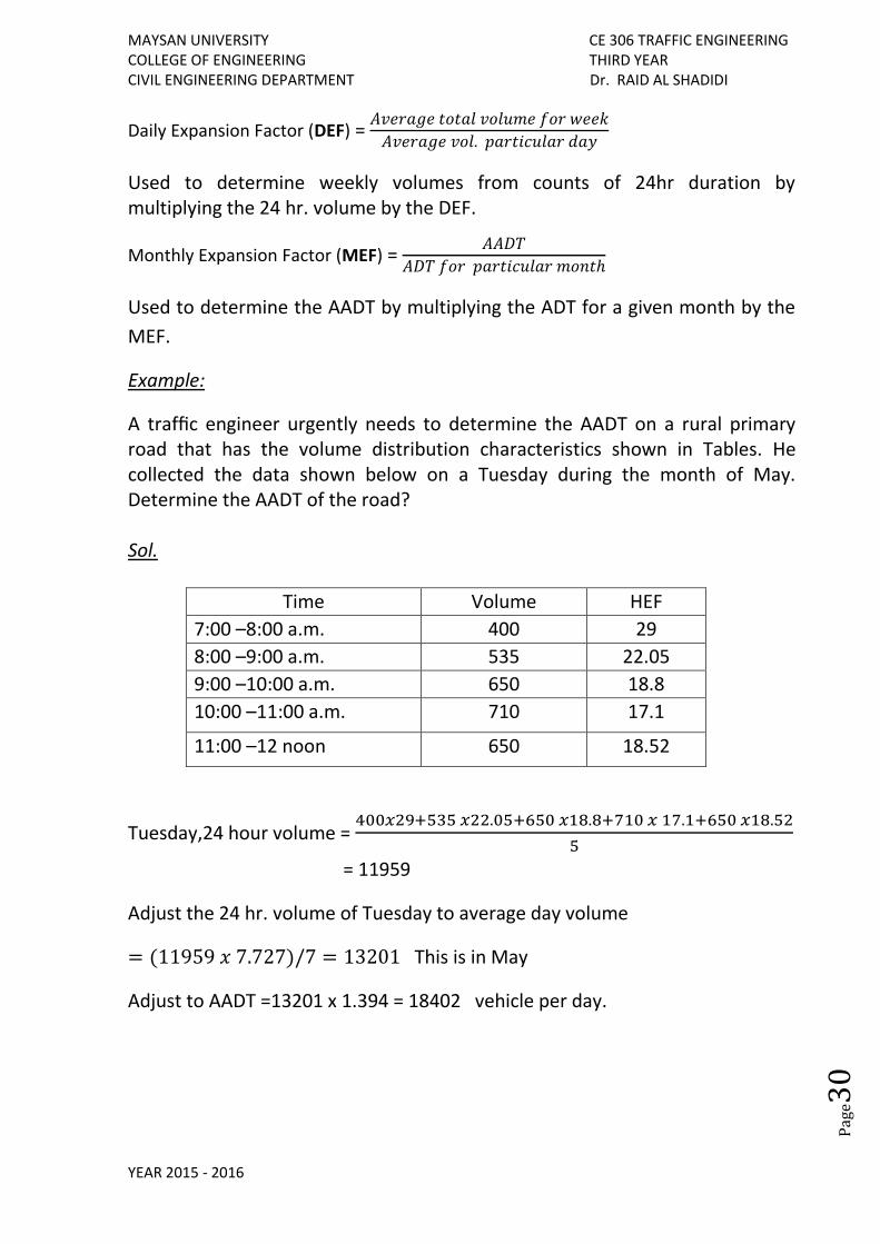
Example:
A traffic engineer urgently needs to determine the AADT on a rural primary road that has the volume distribution characteristics shown in Tables. He collected the data shown below on a Tuesday during the month of May. Determine the AADT of the road? Sol.
Time Volume HEF
7:00 –8:00 a.m. 400 29
8:00 –9:00 a.m. 535 22.05
9:00 –10:00 a.m. 650 18.8
10:00 –11:00 a.m. 710 17.1
11:00 –12 noon 650 18.52
Tuesday,24 hour volume = 400𝑥29+535 𝑥22.05+650 𝑥18.8+710 𝑥 17.1+650 𝑥18.52
5
= 11959
Adjust the 24 hr. volume of Tuesday to average day volume
= (11959 𝑥 7.727)/7 = 13201 This is in May
Adjust to AADT =13201 x 1.394 = 18402 vehicle per day.
MAYSAN UNIVERSITY CE 306 TRAFFIC ENGINEERING COLLEGE OF ENGINEERING THIRD YEAR CIVIL ENGINEERING DEPARTMENT Dr. RAID AL SHADIDI
YEAR 2015 - 2016
Pag
e31
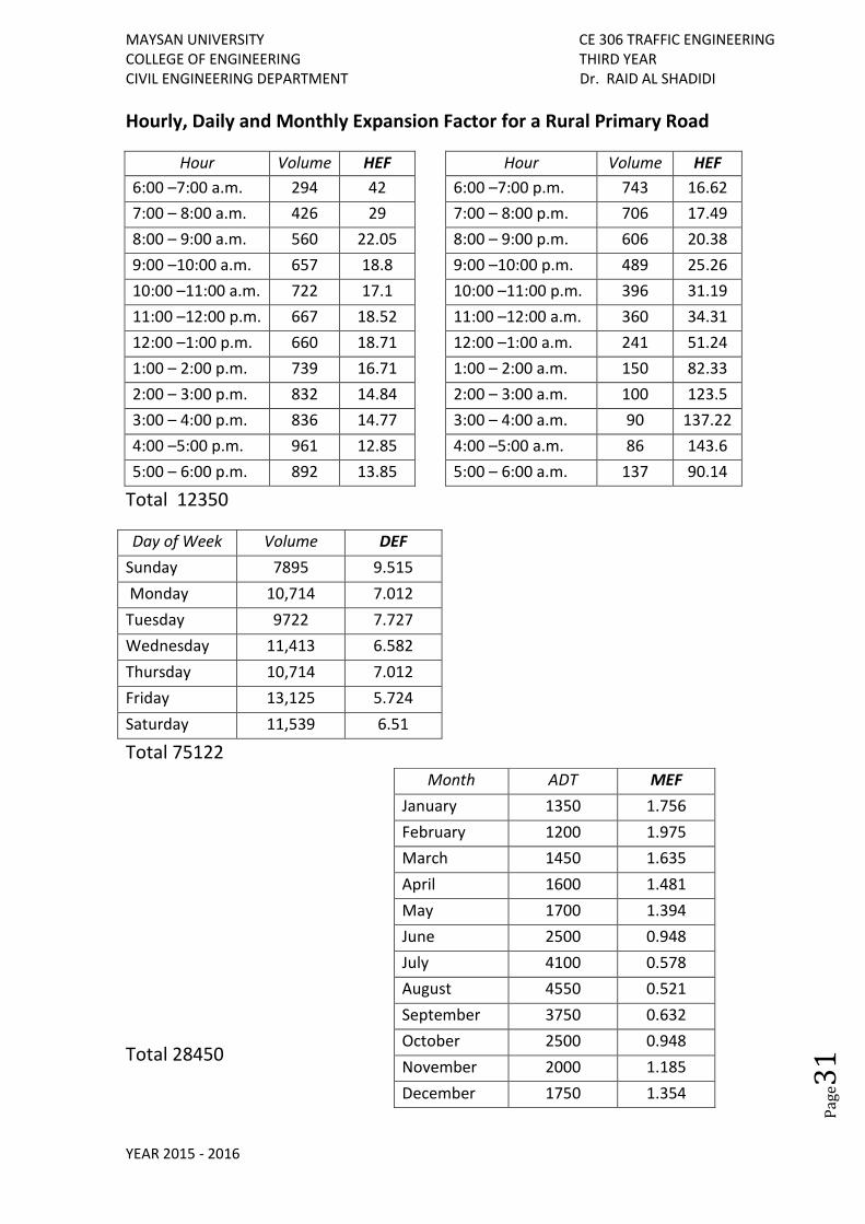
Hourly, Daily and Monthly Expansion Factor for a Rural Primary Road
Hour Volume HEF Hour Volume HEF
6:00 –7:00 a.m. 294 42 6:00 –7:00 p.m. 743 16.62
7:00 – 8:00 a.m. 426 29 7:00 – 8:00 p.m. 706 17.49
8:00 – 9:00 a.m. 560 22.05 8:00 – 9:00 p.m. 606 20.38
9:00 –10:00 a.m. 657 18.8 9:00 –10:00 p.m. 489 25.26
10:00 –11:00 a.m. 722 17.1 10:00 –11:00 p.m. 396 31.19
11:00 –12:00 p.m. 667 18.52 11:00 –12:00 a.m. 360 34.31
12:00 –1:00 p.m. 660 18.71 12:00 –1:00 a.m. 241 51.24
1:00 – 2:00 p.m. 739 16.71 1:00 – 2:00 a.m. 150 82.33
2:00 – 3:00 p.m. 832 14.84 2:00 – 3:00 a.m. 100 123.5
3:00 – 4:00 p.m. 836 14.77 3:00 – 4:00 a.m. 90 137.22
4:00 –5:00 p.m. 961 12.85 4:00 –5:00 a.m. 86 143.6
5:00 – 6:00 p.m. 892 13.85 5:00 – 6:00 a.m. 137 90.14
Total 12350
Day of Week Volume DEF
Sunday 7895 9.515
Monday 10,714 7.012
Tuesday 9722 7.727
Wednesday 11,413 6.582
Thursday 10,714 7.012
Friday 13,125 5.724
Saturday 11,539 6.51
Total 75122
Total 28450
Month ADT MEF
January 1350 1.756
February 1200 1.975
March 1450 1.635
April 1600 1.481
May 1700 1.394
June 2500 0.948
July 4100 0.578
August 4550 0.521
September 3750 0.632
October 2500 0.948
November 2000 1.185
December 1750 1.354
MAYSAN UNIVERSITY CE 306 TRAFFIC ENGINEERING COLLEGE OF ENGINEERING THIRD YEAR CIVIL ENGINEERING DEPARTMENT Dr. RAID AL SHADIDI
YEAR 2015 - 2016
Pag
e32
Fundamental Principles of Traffic Flow
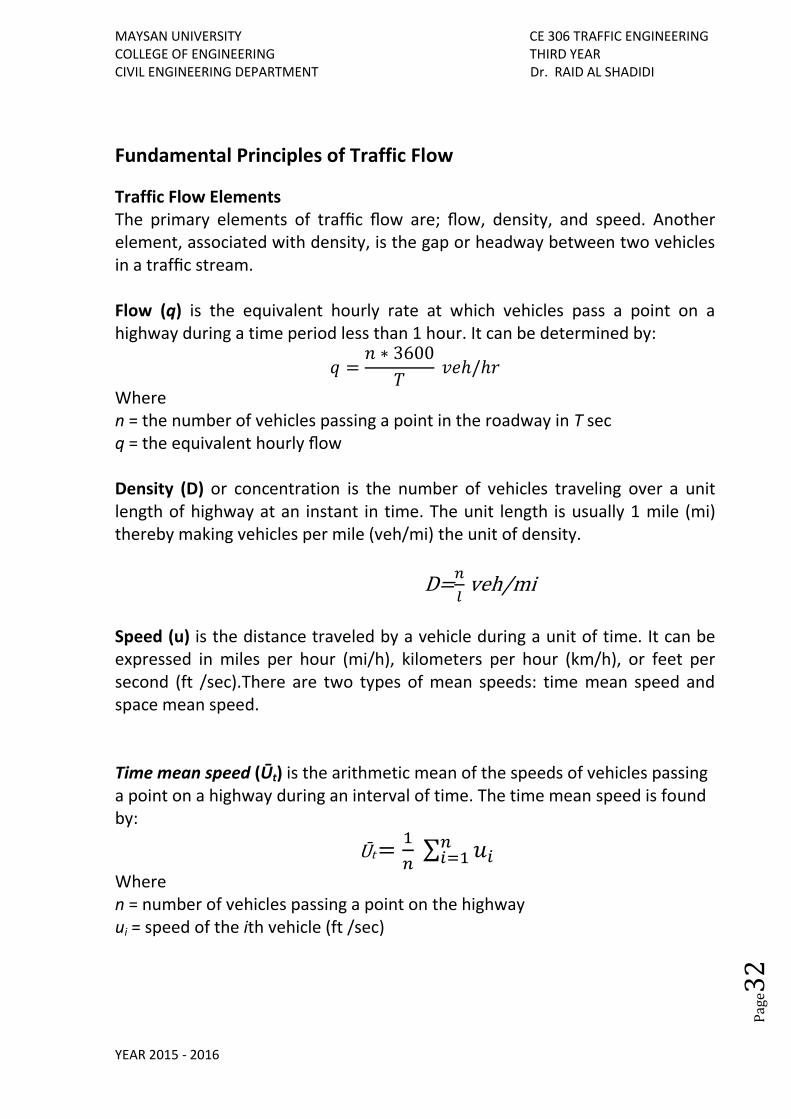
Traffic Flow Elements The primary elements of traffic flow are; flow, density, and speed. Another element, associated with density, is the gap or headway between two vehicles in a traffic stream. Flow (q) is the equivalent hourly rate at which vehicles pass a point on a highway during a time period less than 1 hour. It can be determined by:
𝑞 =𝑛 ∗ 3600
𝑇 𝑣𝑒ℎ/ℎ𝑟
Where n = the number of vehicles passing a point in the roadway in T sec q = the equivalent hourly flow Density (D) or concentration is the number of vehicles traveling over a unit length of highway at an instant in time. The unit length is usually 1 mile (mi) thereby making vehicles per mile (veh/mi) the unit of density.
D=𝑛
𝑙 veh/mi
Speed (u) is the distance traveled by a vehicle during a unit of time. It can be expressed in miles per hour (mi/h), kilometers per hour (km/h), or feet per second (ft /sec).There are two types of mean speeds: time mean speed and space mean speed. Time mean speed (Ūt) is the arithmetic mean of the speeds of vehicles passing a point on a highway during an interval of time. The time mean speed is found by:
Ūt =1
𝑛 ∑ 𝑢𝑖
𝑛𝑖=1
Where n = number of vehicles passing a point on the highway ui = speed of the ith vehicle (ft /sec)
MAYSAN UNIVERSITY CE 306 TRAFFIC ENGINEERING COLLEGE OF ENGINEERING THIRD YEAR CIVIL ENGINEERING DEPARTMENT Dr. RAID AL SHADIDI
YEAR 2015 - 2016
Pag
e33
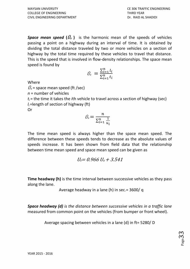
Space mean speed (Ūs ) is the harmonic mean of the speeds of vehicles passing a point on a highway during an interval of time. It is obtained by dividing the total distance traveled by two or more vehicles on a section of highway by the total time required by these vehicles to travel that distance. This is the speed that is involved in flow-density relationships. The space mean speed is found by
Ūs =∑ 𝑙𝑖
𝑛𝑖=1
∑ 𝑡𝑖𝑛𝑖=1
Where Ūs = space mean speed (ft /sec) n = number of vehicles ti = the time it takes the ith vehicle to travel across a section of highway (sec) li =length of section of highway (ft) Or
Ūs =𝑛
∑ 1
𝑢𝑖
𝑛𝑖=1
The time mean speed is always higher than the space mean speed. The difference between these speeds tends to decrease as the absolute values of speeds increase. It has been shown from field data that the relationship between time mean speed and space mean speed can be given as
Ut= 0.966 Us + 3.541
Time headway (h) is the time interval between successive vehicles as they pass along the lane. Average headway in a lane (h) in sec.= 3600/ q Space headway (d) is the distance between successive vehicles in a traffic lane measured from common point on the vehicles (from bumper or front wheel).
Average spacing between vehicles in a lane (d) in ft= 5280/ D
MAYSAN UNIVERSITY CE 306 TRAFFIC ENGINEERING COLLEGE OF ENGINEERING THIRD YEAR CIVIL ENGINEERING DEPARTMENT Dr. RAID AL SHADIDI
YEAR 2015 - 2016
Pag
e34
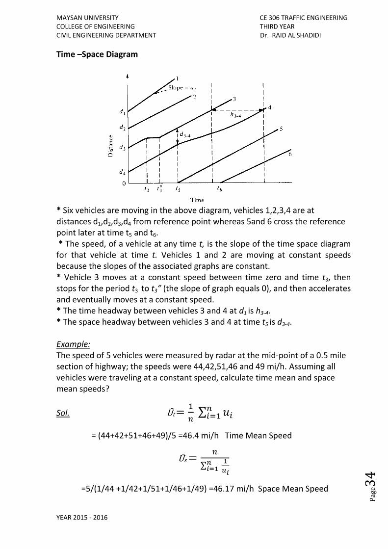
Time –Space Diagram * Six vehicles are moving in the above diagram, vehicles 1,2,3,4 are at distances d1,d2,d3,d4 from reference point whereas 5and 6 cross the reference point later at time t5 and t6. * The speed, of a vehicle at any time t, is the slope of the time space diagram for that vehicle at time t. Vehicles 1 and 2 are moving at constant speeds because the slopes of the associated graphs are constant. * Vehicle 3 moves at a constant speed between time zero and time t3, then stops for the period t3 to t3” (the slope of graph equals 0), and then accelerates and eventually moves at a constant speed. * The time headway between vehicles 3 and 4 at d1 is h3-4. * The space headway between vehicles 3 and 4 at time t5 is d3-4. Example: The speed of 5 vehicles were measured by radar at the mid-point of a 0.5 mile section of highway; the speeds were 44,42,51,46 and 49 mi/h. Assuming all vehicles were traveling at a constant speed, calculate time mean and space mean speeds?
Sol. Ūt =1
𝑛 ∑ 𝑢𝑖
𝑛𝑖=1
= (44+42+51+46+49)/5 =46.4 mi/h Time Mean Speed
Ūs =𝑛
∑ 1
𝑢𝑖
𝑛𝑖=1
=5/(1/44 +1/42+1/51+1/46+1/49) =46.17 mi/h Space Mean Speed
MAYSAN UNIVERSITY CE 306 TRAFFIC ENGINEERING COLLEGE OF ENGINEERING THIRD YEAR CIVIL ENGINEERING DEPARTMENT Dr. RAID AL SHADIDI
YEAR 2015 - 2016
Pag
e35
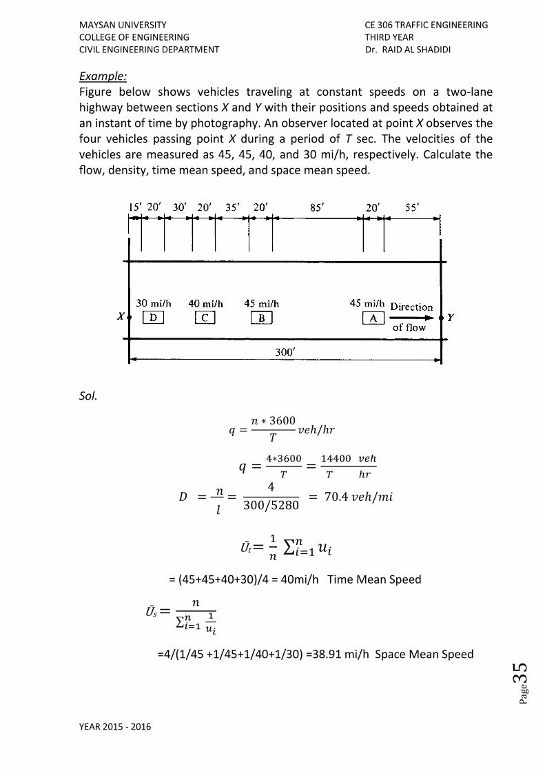
Example: Figure below shows vehicles traveling at constant speeds on a two-lane highway between sections X and Y with their positions and speeds obtained at an instant of time by photography. An observer located at point X observes the four vehicles passing point X during a period of T sec. The velocities of the vehicles are measured as 45, 45, 40, and 30 mi/h, respectively. Calculate the flow, density, time mean speed, and space mean speed.
Sol.
𝑞 =𝑛 ∗ 3600
𝑇𝑣𝑒ℎ/ℎ𝑟
𝑞 =4∗3600
𝑇=
14400 𝑣𝑒ℎ
𝑇 ℎ𝑟
𝐷 =
𝑛 𝑙
= 4
300/5280 = 70.4 𝑣𝑒ℎ/𝑚𝑖
Ūt =1
𝑛 ∑ 𝑢𝑖
𝑛𝑖=1
= (45+45+40+30)/4 = 40mi/h Time Mean Speed
Ūs =𝑛
∑ 1
𝑢𝑖
𝑛𝑖=1
=4/(1/45 +1/45+1/40+1/30) =38.91 mi/h Space Mean Speed
MAYSAN UNIVERSITY CE 306 TRAFFIC ENGINEERING COLLEGE OF ENGINEERING THIRD YEAR CIVIL ENGINEERING DEPARTMENT Dr. RAID AL SHADIDI
YEAR 2015 - 2016
Pag
e36
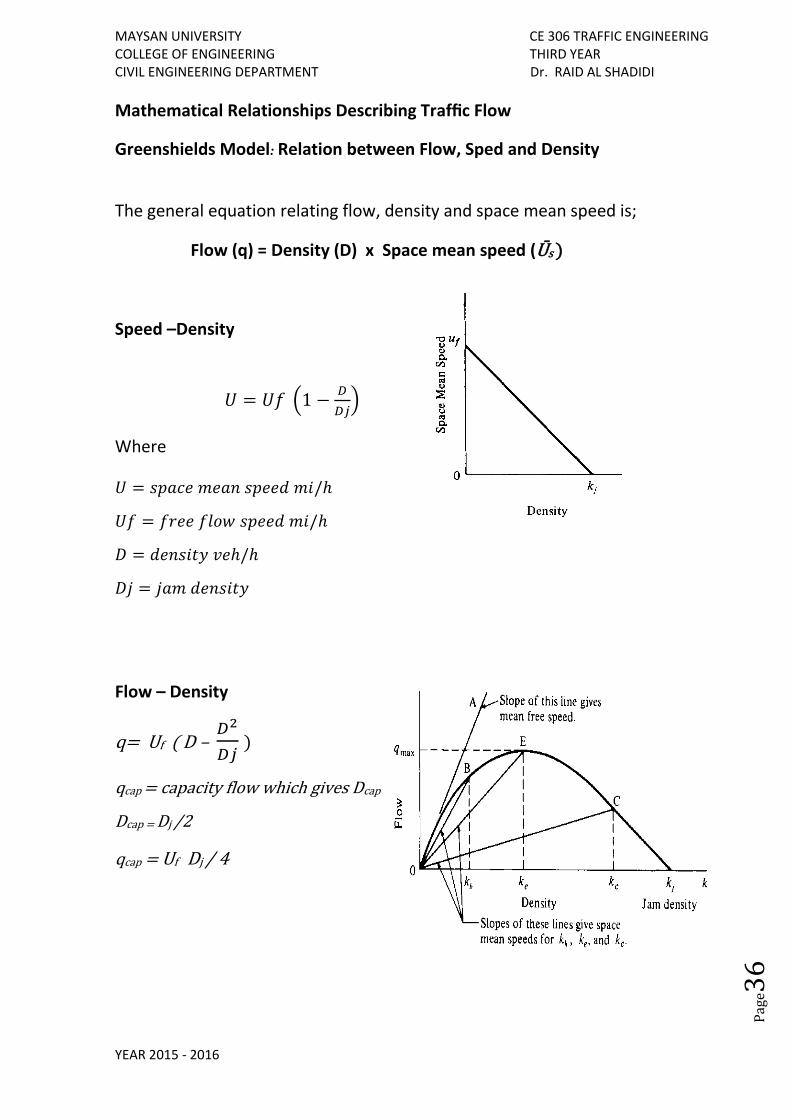
Mathematical Relationships Describing Traffic Flow
Greenshields Model: Relation between Flow, Sped and Density
The general equation relating flow, density and space mean speed is;
Flow (q) = Density (D) x Space mean speed (Ūs )
Speed –Density
𝑈 = 𝑈𝑓 (1 −𝐷
𝐷𝑗)
Where
𝑈 = 𝑠𝑝𝑎𝑐𝑒 𝑚𝑒𝑎𝑛 𝑠𝑝𝑒𝑒𝑑 𝑚𝑖/ℎ
𝑈𝑓 = 𝑓𝑟𝑒𝑒 𝑓𝑙𝑜𝑤 𝑠𝑝𝑒𝑒𝑑 𝑚𝑖/ℎ
𝐷 = 𝑑𝑒𝑛𝑠𝑖𝑡𝑦 𝑣𝑒ℎ/ℎ
𝐷𝑗 = 𝑗𝑎𝑚 𝑑𝑒𝑛𝑠𝑖𝑡𝑦
Flow – Density
q= Uf ( D – 𝐷2
𝐷𝑗 )
qcap = capacity flow which gives Dcap
Dcap = Dj /2
qcap = Uf Dj / 4
MAYSAN UNIVERSITY CE 306 TRAFFIC ENGINEERING COLLEGE OF ENGINEERING THIRD YEAR CIVIL ENGINEERING DEPARTMENT Dr. RAID AL SHADIDI
YEAR 2015 - 2016
Pag
e37
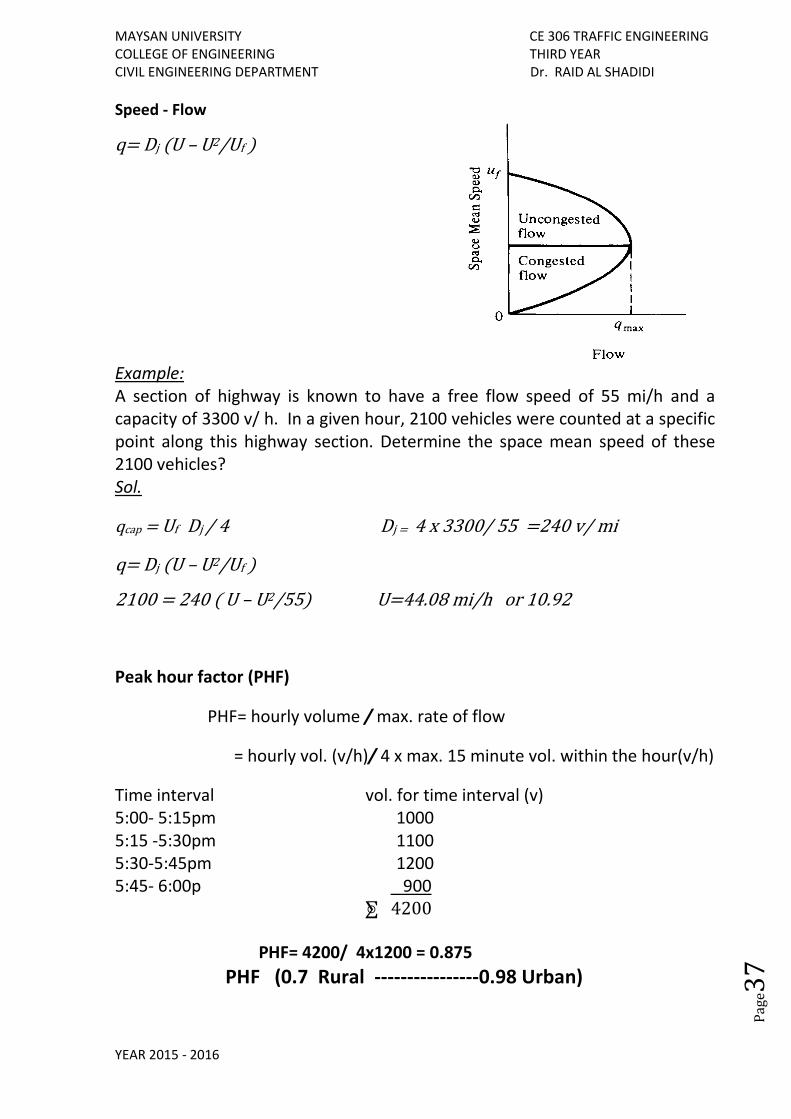
Speed - Flow
q= Dj (U – U2/Uf )
Example: A section of highway is known to have a free flow speed of 55 mi/h and a capacity of 3300 v/ h. In a given hour, 2100 vehicles were counted at a specific point along this highway section. Determine the space mean speed of these 2100 vehicles? Sol.
qcap = Uf Dj / 4 Dj = 4 x 3300/ 55 =240 v/ mi
q= Dj (U – U2/Uf )
2100 = 240 ( U – U2/55) U=44.08 mi/h or 10.92
Peak hour factor (PHF)
PHF= hourly volume / max. rate of flow
= hourly vol. (v/h)/ 4 x max. 15 minute vol. within the hour(v/h)
Time interval vol. for time interval (v) 5:00- 5:15pm 1000 5:15 -5:30pm 1100 5:30-5:45pm 1200 5:45- 6:00p 900 ⨊ 4200 PHF= 4200/ 4x1200 = 0.875
PHF (0.7 Rural ----------------0.98 Urban)
MAYSAN UNIVERSITY CE 306 TRAFFIC ENGINEERING COLLEGE OF ENGINEERING THIRD YEAR CIVIL ENGINEERING DEPARTMENT Dr. RAID AL SHADIDI
YEAR 2015 - 2016
Pag
e38
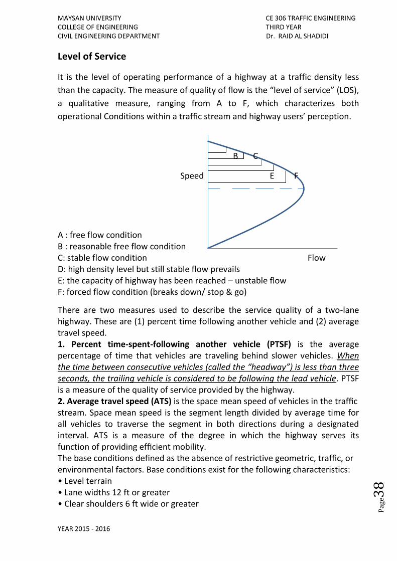
Level of Service
It is the level of operating performance of a highway at a traffic density less
than the capacity. The measure of quality of flow is the “level of service” (LOS),
a qualitative measure, ranging from A to F, which characterizes both
operational Conditions within a traffic stream and highway users’ perception.
B C
Speed E F
A : free flow condition B : reasonable free flow condition C: stable flow condition Flow D: high density level but still stable flow prevails E: the capacity of highway has been reached – unstable flow F: forced flow condition (breaks down/ stop & go)
There are two measures used to describe the service quality of a two-lane highway. These are (1) percent time following another vehicle and (2) average travel speed. 1. Percent time-spent-following another vehicle (PTSF) is the average percentage of time that vehicles are traveling behind slower vehicles. When the time between consecutive vehicles (called the “headway”) is less than three seconds, the trailing vehicle is considered to be following the lead vehicle. PTSF is a measure of the quality of service provided by the highway. 2. Average travel speed (ATS) is the space mean speed of vehicles in the traffic stream. Space mean speed is the segment length divided by average time for all vehicles to traverse the segment in both directions during a designated interval. ATS is a measure of the degree in which the highway serves its function of providing efficient mobility. The base conditions defined as the absence of restrictive geometric, traffic, or environmental factors. Base conditions exist for the following characteristics: • Level terrain • Lane widths 12 ft or greater • Clear shoulders 6 ft wide or greater
MAYSAN UNIVERSITY CE 306 TRAFFIC ENGINEERING COLLEGE OF ENGINEERING THIRD YEAR CIVIL ENGINEERING DEPARTMENT Dr. RAID AL SHADIDI
YEAR 2015 - 2016
Pag
e39
• Passing permitted with absence of no-passing zones • No impediments to through traffic due to traffic control or turning vehicles • Passenger cars only in the traffic stream • Equal volume in both directions (for analysis of two-way flow)
Level of Service A: This is the highest quality of service that can be achieved. Motorists are able to travel at their desired speed. The need for passing other vehicles is well below the capacity for passing and few (if any) platoons of three or more cars are observed. Average travel speed (ATS) is 55 mi/h or greater, and travel delays (PTSF) occur no more than 35 percent of the time. Maximum service flow rate (two-way) under base conditions is 490 pc/h. Level of Service B: At this level of service, if vehicles are to maintain desired speeds, the demand for passing other vehicles increases significantly. At the lower level of LOS B range, the passing demand and passing capacity are approximately equal. Average travel speeds (ATS) are 50 to 55 mi/h. Travel delays (PTSF) occur between 35 and 50 percent of the time. Maximum service flow rate (two-way) under base conditions is 780 pc/h. Level of Service C: Further increases in flow beyond the LOS B range results in a noticeable increase in the formation of platoons and an increase in platoon size. Passing opportunities are severely decreased. Average travel speeds (ATS) are 45 to 50 mi/h, and travel delays (PTSF) occur between 50 and 65 percent of the time. Maximum service flow rate (two-way) under base conditions is 1190 pc/h. Level of Service D: Flow is unstable and passing maneuvers are difficult, if not impossible, to complete. Since the number of passing opportunities is approaching zero as passing desires increase, each lane operates essentially independently of the opposing lane. It is not uncommon that platoons will form that are 5 to 10 consecutive vehicles in length. Average travel speeds (ATS) are 40 to 45 mi/h, and travel delays (PTSF) occur between 65 and 80 percent of the time. Maximum service flow rate (two-way) under base conditions is 1830 pc/h. Level of Service E: Passing has become virtually impossible. Platoons are longer and more frequent as slower vehicles are encountered more often. Operating conditions are unstable and are difficult to predict. Average travel speeds (ATS) are 40 mi/h or less and travel delays (PTSF) occur more than 80 percent of the time. Maximum service flow rate (two-way) under base conditions is 3200 pc/h, a value seldom encountered on rural highways (except during summer holiday periods) due to lack of demand. Level of Service F: Traffic is congested with demand exceeding capacity. Volumes are lower than capacity and speeds are variable.
MAYSAN UNIVERSITY CE 306 TRAFFIC ENGINEERING COLLEGE OF ENGINEERING THIRD YEAR CIVIL ENGINEERING DEPARTMENT Dr. RAID AL SHADIDI
YEAR 2015 - 2016
Pag
e40
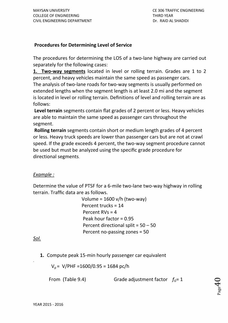
Procedures for Determining Level of Service The procedures for determining the LOS of a two-lane highway are carried out separately for the following cases: 1. Two-way segments located in level or rolling terrain. Grades are 1 to 2 percent, and heavy vehicles maintain the same speed as passenger cars. The analysis of two-lane roads for two-way segments is usually performed on extended lengths when the segment length is at least 2.0 mi and the segment is located in level or rolling terrain. Definitions of level and rolling terrain are as follows: Level terrain segments contain flat grades of 2 percent or less. Heavy vehicles are able to maintain the same speed as passenger cars throughout the segment. Rolling terrain segments contain short or medium length grades of 4 percent or less. Heavy truck speeds are lower than passenger cars but are not at crawl speed. If the grade exceeds 4 percent, the two-way segment procedure cannot be used but must be analyzed using the specific grade procedure for directional segments.
Example :
Determine the value of PTSF for a 6-mile two-lane two-way highway in rolling terrain. Traffic data are as follows. Volume = 1600 v/h (two-way) Percent trucks = 14 Percent RVs = 4 Peak hour factor = 0.95 Percent directional split = 50 – 50 Percent no-passing zones = 50 Sol.
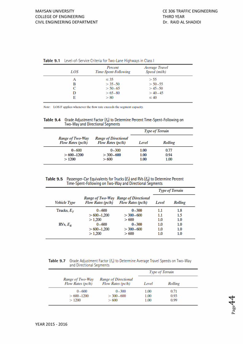
1. Compute peak 15-min hourly passenger car equivalent . Vp = V/PHF =1600/0.95 = 1684 pc/h From (Table 9.4) Grade adjustment factor fG= 1
MAYSAN UNIVERSITY CE 306 TRAFFIC ENGINEERING COLLEGE OF ENGINEERING THIRD YEAR CIVIL ENGINEERING DEPARTMENT Dr. RAID AL SHADIDI
YEAR 2015 - 2016
Pag
e41
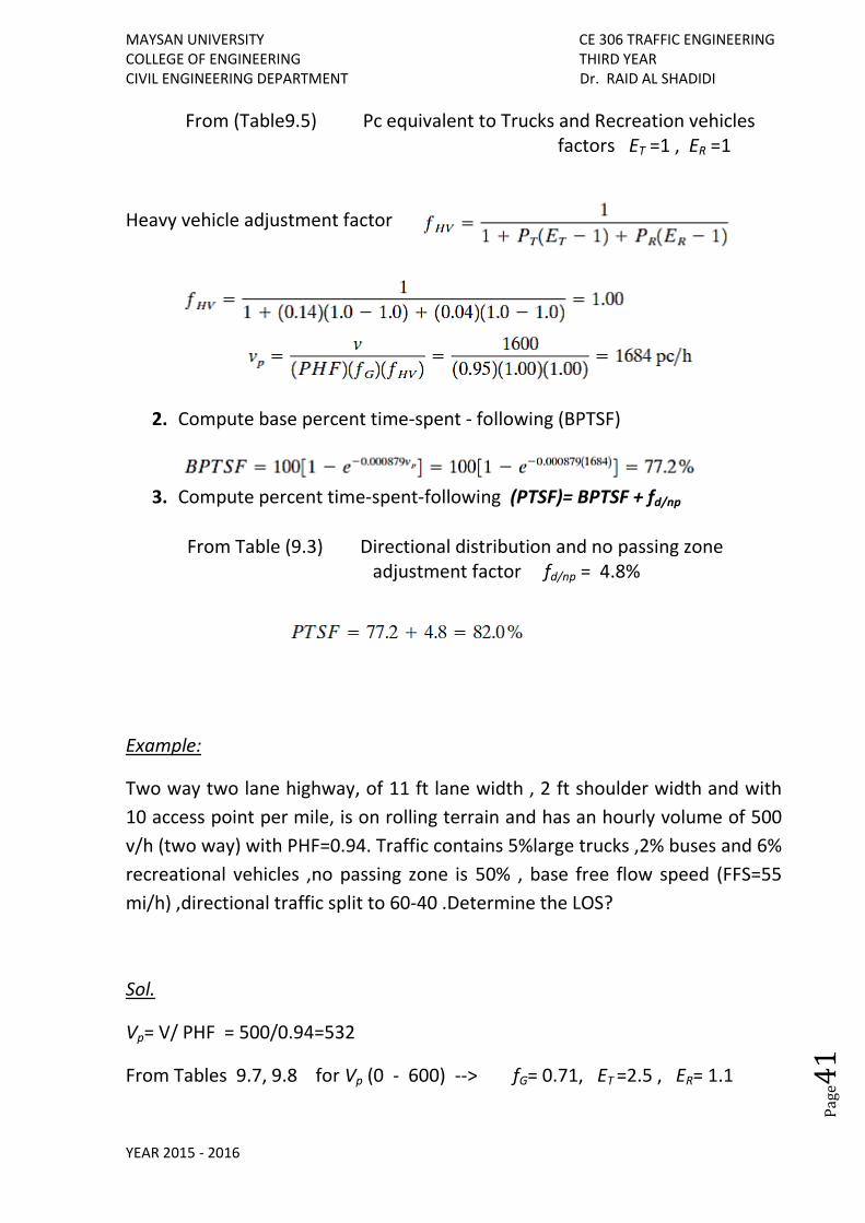
From (Table9.5) Pc equivalent to Trucks and Recreation vehicles factors ET =1 , ER =1
Heavy vehicle adjustment factor
2. Compute base percent time-spent - following (BPTSF)
3. Compute percent time-spent-following (PTSF)= BPTSF + fd/np
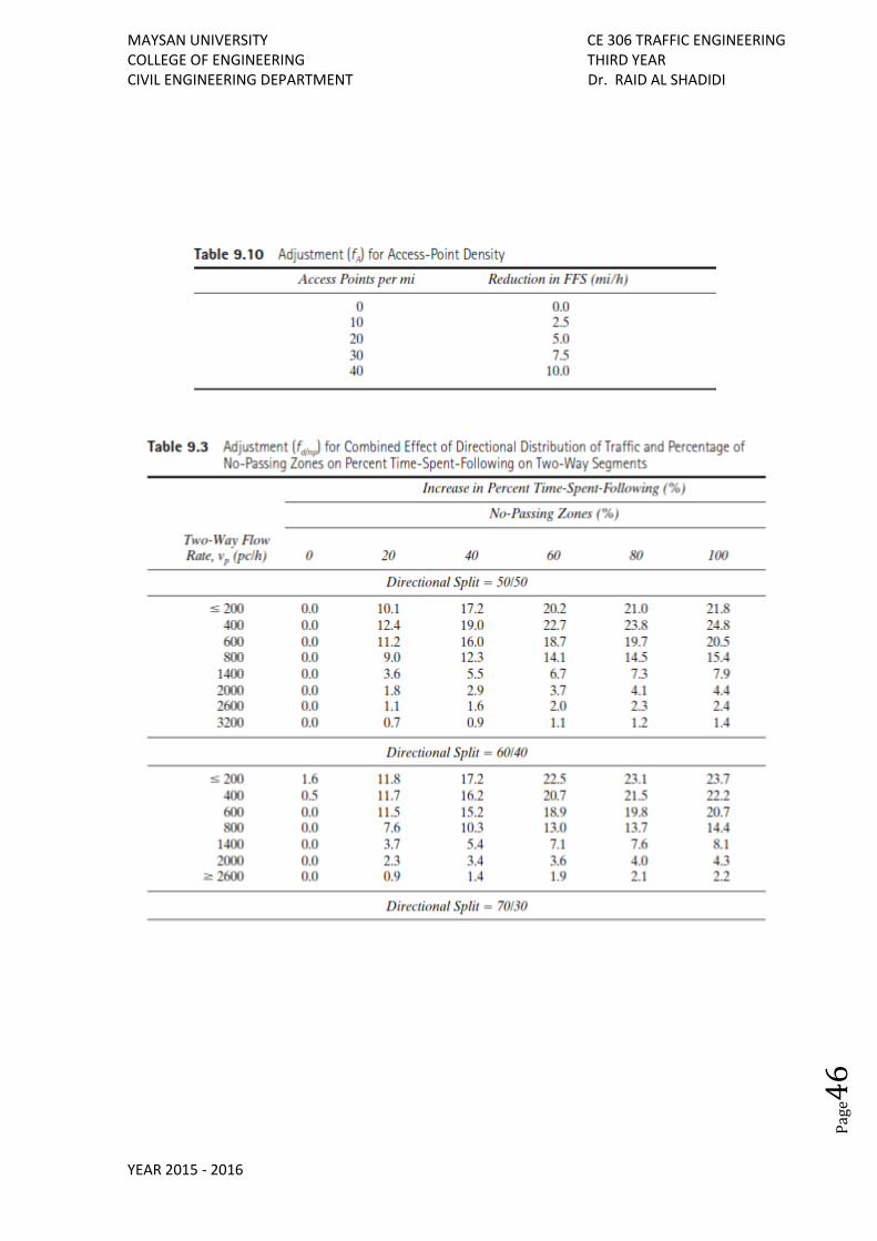
From Table (9.3) Directional distribution and no passing zone adjustment factor fd/np = 4.8%
Example:
Two way two lane highway, of 11 ft lane width , 2 ft shoulder width and with
10 access point per mile, is on rolling terrain and has an hourly volume of 500
v/h (two way) with PHF=0.94. Traffic contains 5%large trucks ,2% buses and 6%
recreational vehicles ,no passing zone is 50% , base free flow speed (FFS=55
mi/h) ,directional traffic split to 60-40 .Determine the LOS?
Sol.
Vp= V/ PHF = 500/0.94=532
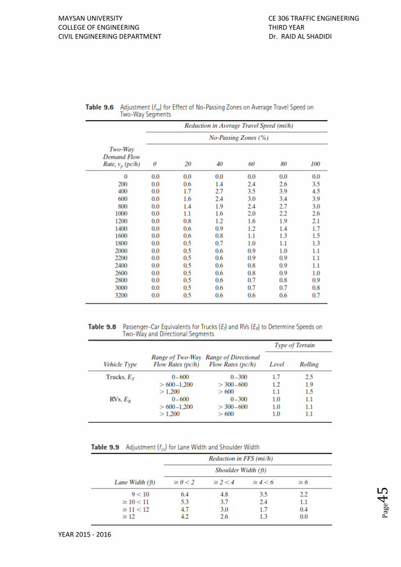
From Tables 9.7, 9.8 for Vp (0 - 600) --> fG= 0.71, ET =2.5 , ER= 1.1
MAYSAN UNIVERSITY CE 306 TRAFFIC ENGINEERING COLLEGE OF ENGINEERING THIRD YEAR CIVIL ENGINEERING DEPARTMENT Dr. RAID AL SHADIDI
YEAR 2015 - 2016
Pag
e42
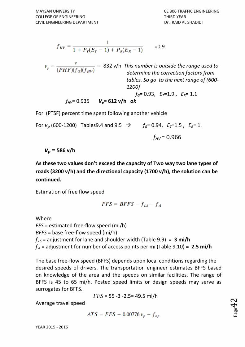
=0.9
832 v/h This number is outside the range used to
determine the correction factors from tables. So go to the next range of (600-1200)
fG= 0.93, ET=1.9 , ER= 1.1 fHV= 0.935 Vp= 612 v/h ok
For (PTSF) percent time spent following another vehicle
For vp (600-1200) Tables9.4 and 9.5 fG= 0.94, ET=1.5 , ER= 1.
fHV = 0.966
vp = 586 v/h
As these two values don’t exceed the capacity of Two way two lane types of
roads (3200 v/h) and the directional capacity (1700 v/h), the solution can be
continued.
Estimation of free flow speed
Where FFS = estimated free-flow speed (mi/h) BFFS = base free-flow speed (mi/h) f LS = adjustment for lane and shoulder width (Table 9.9) = 3 mi/h f A = adjustment for number of access points per mi (Table 9.10) = 2.5 mi/h The base free-flow speed (BFFS) depends upon local conditions regarding the desired speeds of drivers. The transportation engineer estimates BFFS based on knowledge of the area and the speeds on similar facilities. The range of BFFS is 45 to 65 mi/h. Posted speed limits or design speeds may serve as surrogates for BFFS. FFS = 55 -3 -2.5= 49.5 mi/h Average travel speed
MAYSAN UNIVERSITY CE 306 TRAFFIC ENGINEERING COLLEGE OF ENGINEERING THIRD YEAR CIVIL ENGINEERING DEPARTMENT Dr. RAID AL SHADIDI
YEAR 2015 - 2016
Pag
e43
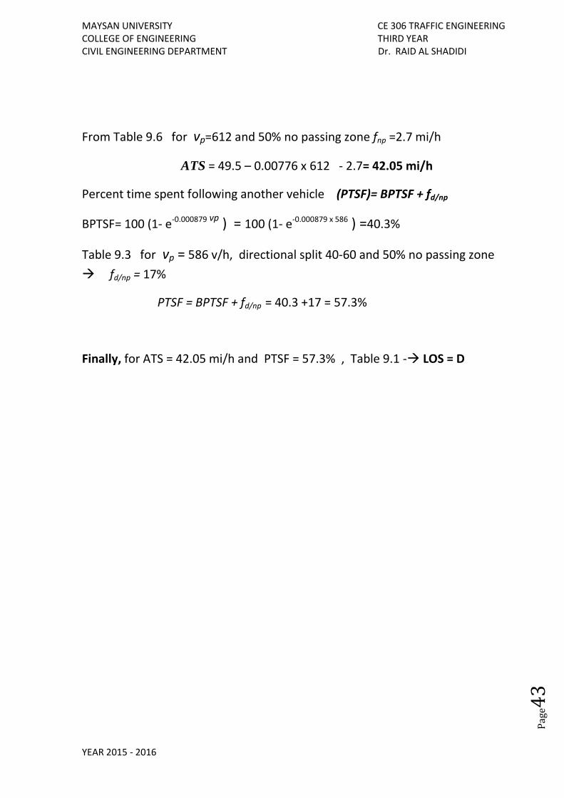
From Table 9.6 for vp=612 and 50% no passing zone fnp =2.7 mi/h
ATS = 49.5 – 0.00776 x 612 - 2.7= 42.05 mi/h
Percent time spent following another vehicle (PTSF)= BPTSF + fd/np
BPTSF= 100 (1- e-0.000879 vp ) = 100 (1- e-0.000879 x 586 ) =40.3%
Table 9.3 for vp = 586 v/h, directional split 40-60 and 50% no passing zone
fd/np = 17%
PTSF = BPTSF + fd/np = 40.3 +17 = 57.3%
Finally, for ATS = 42.05 mi/h and PTSF = 57.3% , Table 9.1 - LOS = D
MAYSAN UNIVERSITY CE 306 TRAFFIC ENGINEERING COLLEGE OF ENGINEERING THIRD YEAR CIVIL ENGINEERING DEPARTMENT Dr. RAID AL SHADIDI
YEAR 2015 - 2016
Pag
e44
MAYSAN UNIVERSITY CE 306 TRAFFIC ENGINEERING COLLEGE OF ENGINEERING THIRD YEAR CIVIL ENGINEERING DEPARTMENT Dr. RAID AL SHADIDI
YEAR 2015 - 2016
Pag
e45
MAYSAN UNIVERSITY CE 306 TRAFFIC ENGINEERING COLLEGE OF ENGINEERING THIRD YEAR CIVIL ENGINEERING DEPARTMENT Dr. RAID AL SHADIDI
YEAR 2015 - 2016
Pag
e46
MAYSAN UNIVERSITY CE 306 TRAFFIC ENGINEERING COLLEGE OF ENGINEERING THIRD YEAR CIVIL ENGINEERING DEPARTMENT Dr. RAID AL SHADIDI
YEAR 2015 - 2016
Pag
e47
Multilane Highway
Example:
A six lane divided highway is on rolling terrain with 2 access point per mile and
has 10 feet lane width with a 5 feet shoulder on the right side and 3 feet
shoulder on the left side .PHF =0.80, and the directional peak hour volume is
3000vph. There are 6% large trucks, 2% busses and 2% recreational vehicles. A
significant percentage of non-familiar roadway users are in the traffic stream
(the diver population adjustment factor is estimated as 0.95). Posted speed
limit is 55 mph. Determine the LOS?
Sol.
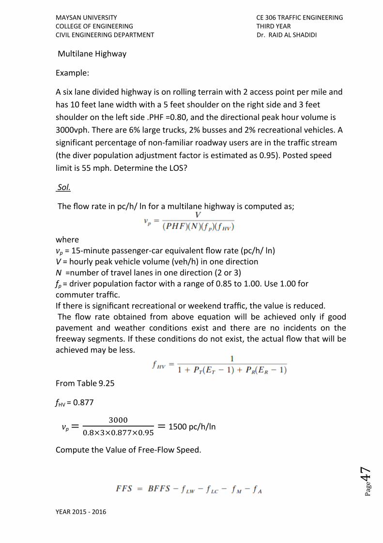
The flow rate in pc/h/ ln for a multilane highway is computed as;
where vp = 15-minute passenger-car equivalent flow rate (pc/h/ ln) V = hourly peak vehicle volume (veh/h) in one direction N =number of travel lanes in one direction (2 or 3) fp = driver population factor with a range of 0.85 to 1.00. Use 1.00 for commuter traffic. If there is significant recreational or weekend traffic, the value is reduced. The flow rate obtained from above equation will be achieved only if good pavement and weather conditions exist and there are no incidents on the freeway segments. If these conditions do not exist, the actual flow that will be achieved may be less.
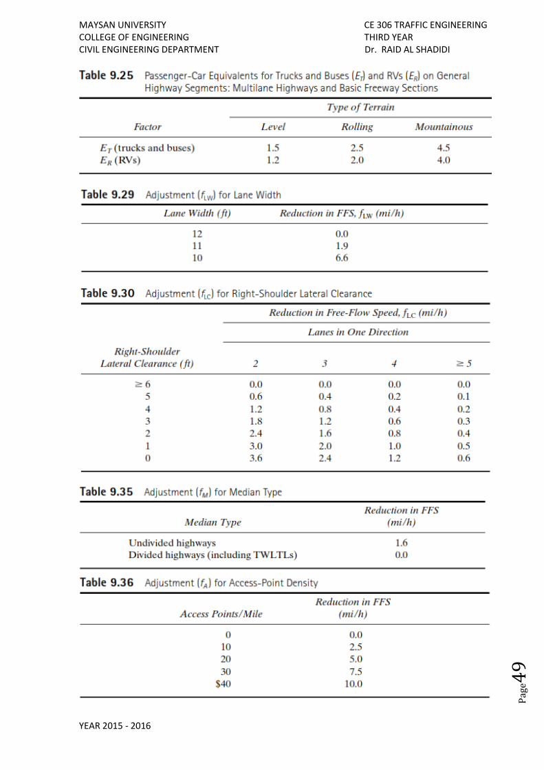
From Table 9.25
fHV = 0.877
vp =3000
0.8×3×0.877×0.95= 1500 pc/h/ln
Compute the Value of Free-Flow Speed.
MAYSAN UNIVERSITY CE 306 TRAFFIC ENGINEERING COLLEGE OF ENGINEERING THIRD YEAR CIVIL ENGINEERING DEPARTMENT Dr. RAID AL SHADIDI
YEAR 2015 - 2016
Pag
e48
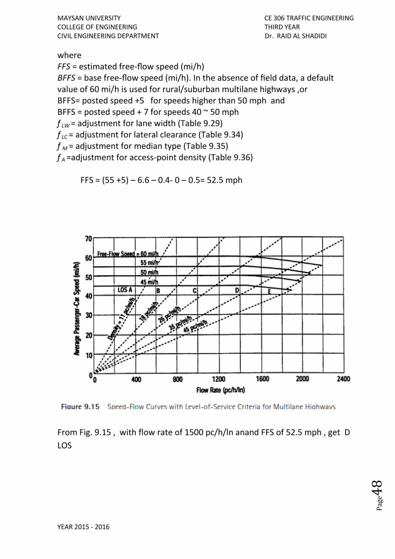
where FFS = estimated free-flow speed (mi/h) BFFS = base free-flow speed (mi/h). In the absence of field data, a default value of 60 mi/h is used for rural/suburban multilane highways ,or BFFS= posted speed +5 for speeds higher than 50 mph and BFFS = posted speed + 7 for speeds 40 ~ 50 mph f LW = adjustment for lane width (Table 9.29) f LC = adjustment for lateral clearance (Table 9.34) f M = adjustment for median type (Table 9.35) f A =adjustment for access-point density (Table 9.36)
FFS = (55 +5) – 6.6 – 0.4- 0 – 0.5= 52.5 mph
From Fig. 9.15 , with flow rate of 1500 pc/h/ln anand FFS of 52.5 mph , get D
LOS
MAYSAN UNIVERSITY CE 306 TRAFFIC ENGINEERING COLLEGE OF ENGINEERING THIRD YEAR CIVIL ENGINEERING DEPARTMENT Dr. RAID AL SHADIDI
YEAR 2015 - 2016
Pag
e49
MAYSAN UNIVERSITY CE 306 TRAFFIC ENGINEERING COLLEGE OF ENGINEERING THIRD YEAR CIVIL ENGINEERING DEPARTMENT Dr. RAID AL SHADIDI
YEAR 2015 - 2016
Pag
e50
Freeway
Example:
A six lane urban freeway is on rolling terrain with 11feet lane width, obstruction 2 feet from the right edge of the traveled pavement and 1.5 interchange per mile. The traffic stream consists of primarily commuters. A directional weekday peak-hour volume of 2200vehicle is observed with 700 vehicles arriving in the most congested 15-minutes period .If the traffic stream has 15% large trucks and buses and no recreational vehicles. Determine the LOS?
Sol.
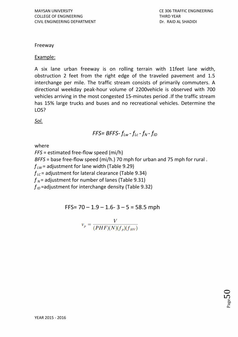
FFS= BFFS- fLw - fLc - fN - fID
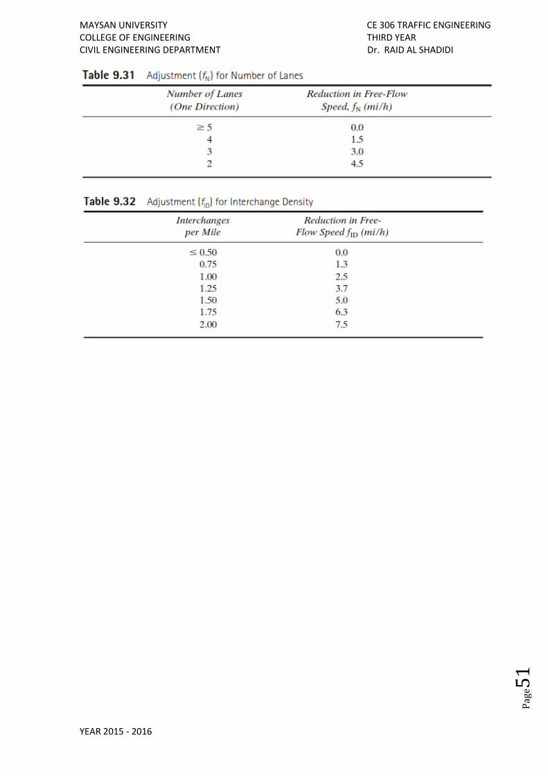
where FFS = estimated free-flow speed (mi/h) BFFS = base free-flow speed (mi/h.) 70 mph for urban and 75 mph for rural . f LW = adjustment for lane width (Table 9.29) f LC = adjustment for lateral clearance (Table 9.34) f N = adjustment for number of lanes (Table 9.31) f ID =adjustment for interchange density (Table 9.32)
FFS= 70 – 1.9 – 1.6- 3 – 5 = 58.5 mph
MAYSAN UNIVERSITY CE 306 TRAFFIC ENGINEERING COLLEGE OF ENGINEERING THIRD YEAR CIVIL ENGINEERING DEPARTMENT Dr. RAID AL SHADIDI
YEAR 2015 - 2016
Pag
e51
MAYSAN UNIVERSITY CE 306 TRAFFIC ENGINEERING COLLEGE OF ENGINEERING THIRD YEAR CIVIL ENGINEERING DEPARTMENT Dr. RAID AL SHADIDI
YEAR 2015 - 2016
Pag
e52
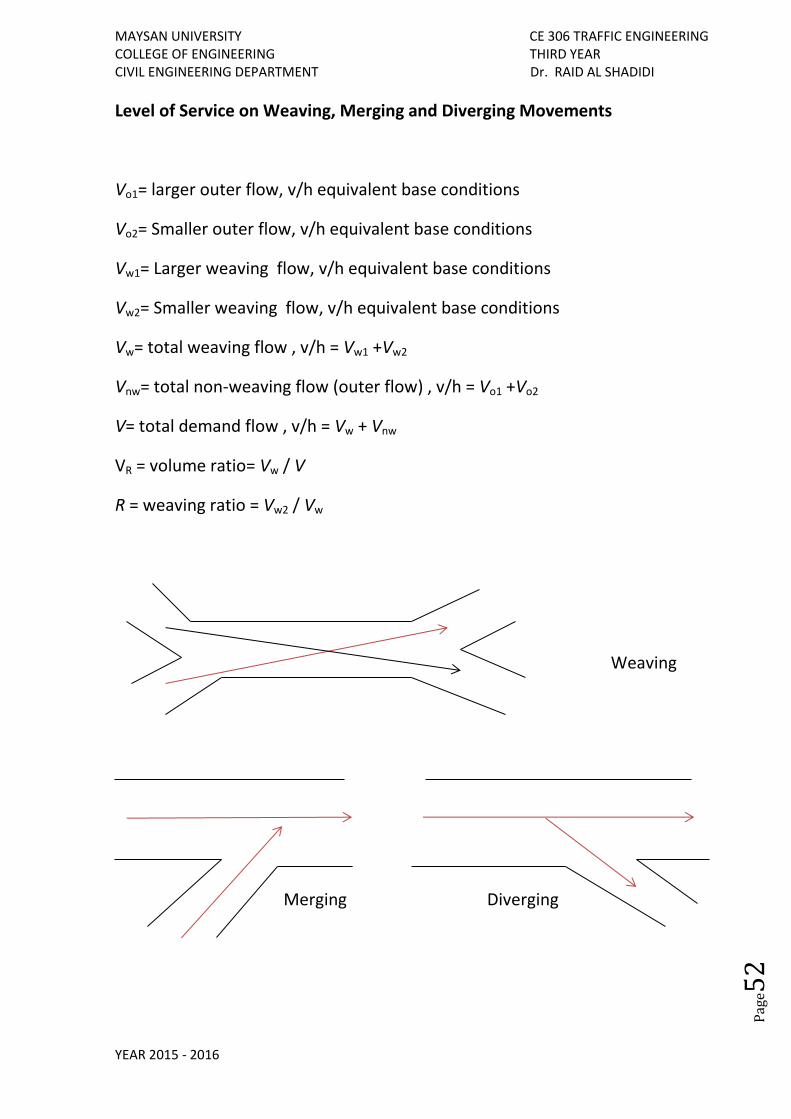
Level of Service on Weaving, Merging and Diverging Movements
Vo1= larger outer flow, v/h equivalent base conditions
Vo2= Smaller outer flow, v/h equivalent base conditions
Vw1= Larger weaving flow, v/h equivalent base conditions
Vw2= Smaller weaving flow, v/h equivalent base conditions
Vw= total weaving flow , v/h = Vw1 +Vw2
Vnw= total non-weaving flow (outer flow) , v/h = Vo1 +Vo2
V= total demand flow , v/h = Vw + Vnw
VR = volume ratio= Vw / V
R = weaving ratio = Vw2 / Vw
Weaving
Merging Diverging
MAYSAN UNIVERSITY CE 306 TRAFFIC ENGINEERING COLLEGE OF ENGINEERING THIRD YEAR CIVIL ENGINEERING DEPARTMENT Dr. RAID AL SHADIDI
YEAR 2015 - 2016
Pag
e53
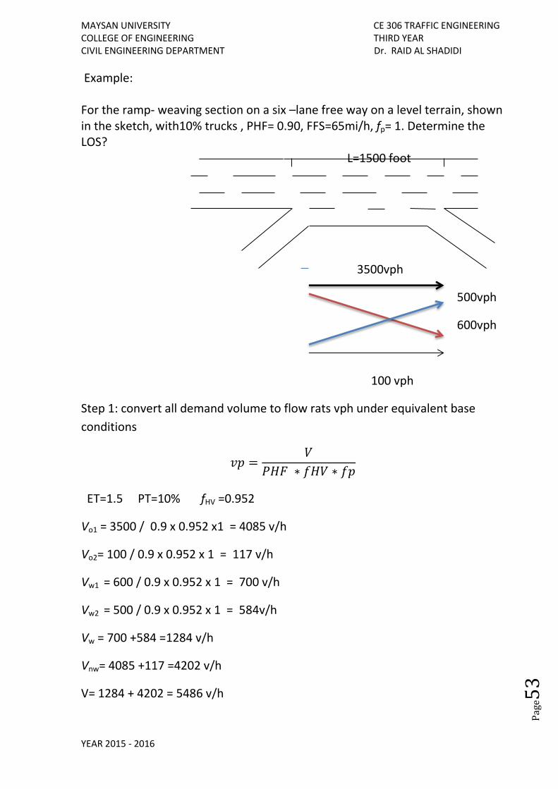
Example: For the ramp- weaving section on a six –lane free way on a level terrain, shown in the sketch, with10% trucks , PHF= 0.90, FFS=65mi/h, fp= 1. Determine the LOS? L=1500 foot
3500vph
500vph
600vph
100 vph
Step 1: convert all demand volume to flow rats vph under equivalent base
conditions
𝑣𝑝 =𝑉
𝑃𝐻𝐹 ∗ 𝑓𝐻𝑉 ∗ 𝑓𝑝
ET=1.5 PT=10% fHV =0.952
Vo1 = 3500 / 0.9 x 0.952 x1 = 4085 v/h
Vo2= 100 / 0.9 x 0.952 x 1 = 117 v/h
Vw1 = 600 / 0.9 x 0.952 x 1 = 700 v/h
Vw2 = 500 / 0.9 x 0.952 x 1 = 584v/h
Vw = 700 +584 =1284 v/h
Vnw= 4085 +117 =4202 v/h
V= 1284 + 4202 = 5486 v/h
MAYSAN UNIVERSITY CE 306 TRAFFIC ENGINEERING COLLEGE OF ENGINEERING THIRD YEAR CIVIL ENGINEERING DEPARTMENT Dr. RAID AL SHADIDI
YEAR 2015 - 2016
Pag
e54
V/ N = 5486/ 4 = 1372 v/h
VR = 1284 / 5486 = 0.23
From sketch L= 1500 foot
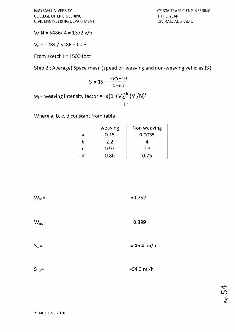
Step 2 : Average( Space mean )speed of weaving and non-weaving vehicles (Si)
Si = 15 + 𝐹𝐹𝑆−10
1+𝑤𝑖
wi = weaving intensity factor = a(1 +VR)b (V /N)c
Ld
Where a, b, c, d constant from table
weaving Non weaving a 0.15 0.0035
b 2.2 4 c 0.97 1.3
d 0.80 0.75
Ww = =0.752
Wnw= =0.399
Sw= = 46.4 mi/h
Snw= =54.3 mi/h
MAYSAN UNIVERSITY CE 306 TRAFFIC ENGINEERING COLLEGE OF ENGINEERING THIRD YEAR CIVIL ENGINEERING DEPARTMENT Dr. RAID AL SHADIDI
YEAR 2015 - 2016
Pag
e55
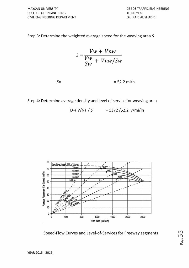
Step 3: Determine the weighted average speed for the weaving area S
𝑆 =𝑉𝑤 + 𝑉𝑛𝑤
𝑉𝑤𝑆𝑤
+ 𝑉𝑛𝑤/𝑆𝑤
S= = 52.2 mi/h
Step 4: Determine average density and level of service for weaving area
D=( V/N) / S = 1372 /52.2 v/mi/ln
Speed-Flow Curves and Level-of-Services for Freeway segments
MAYSAN UNIVERSITY CE 306 TRAFFIC ENGINEERING COLLEGE OF ENGINEERING THIRD YEAR CIVIL ENGINEERING DEPARTMENT Dr. RAID AL SHADIDI
YEAR 2015 - 2016
Pag
e56
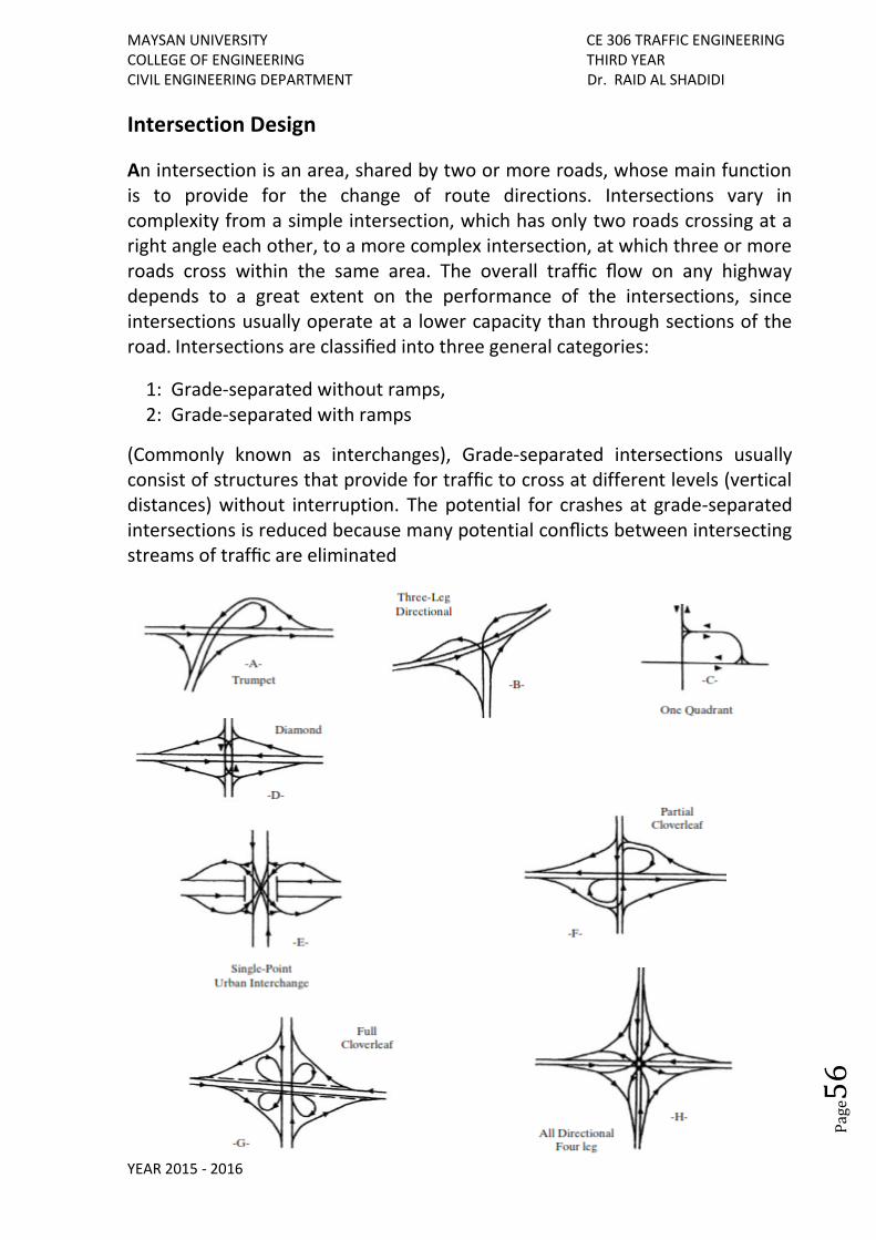
Intersection Design
An intersection is an area, shared by two or more roads, whose main function is to provide for the change of route directions. Intersections vary in complexity from a simple intersection, which has only two roads crossing at a right angle each other, to a more complex intersection, at which three or more roads cross within the same area. The overall traffic flow on any highway depends to a great extent on the performance of the intersections, since intersections usually operate at a lower capacity than through sections of the road. Intersections are classified into three general categories:
1: Grade-separated without ramps, 2: Grade-separated with ramps
(Commonly known as interchanges), Grade-separated intersections usually consist of structures that provide for traffic to cross at different levels (vertical distances) without interruption. The potential for crashes at grade-separated intersections is reduced because many potential conflicts between intersecting streams of traffic are eliminated
MAYSAN UNIVERSITY CE 306 TRAFFIC ENGINEERING COLLEGE OF ENGINEERING THIRD YEAR CIVIL ENGINEERING DEPARTMENT Dr. RAID AL SHADIDI
YEAR 2015 - 2016
Pag
e57
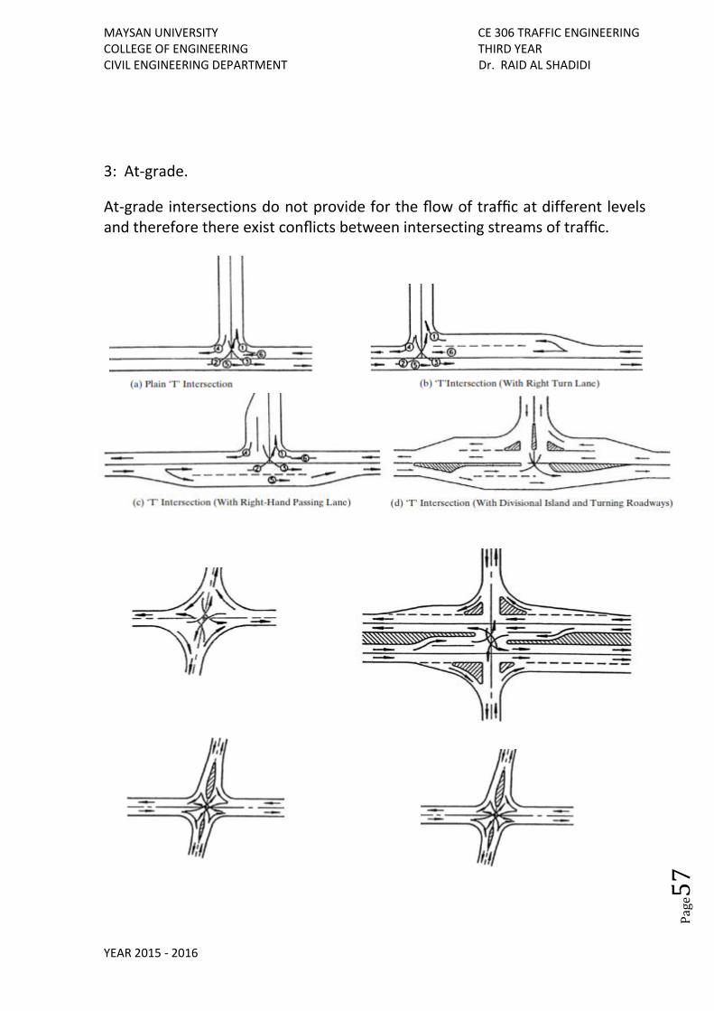
3: At-grade.
At-grade intersections do not provide for the flow of traffic at different levels and therefore there exist conflicts between intersecting streams of traffic.
MAYSAN UNIVERSITY CE 306 TRAFFIC ENGINEERING COLLEGE OF ENGINEERING THIRD YEAR CIVIL ENGINEERING DEPARTMENT Dr. RAID AL SHADIDI
YEAR 2015 - 2016
Pag
e58
Design Principles for At- Grade Intersections
The fundamental objective in the design of at-grade intersections is to minimize the severity of potential conflicts among different streams of traffic and between pedestrians and turning vehicles. At the same time, it is necessary to provide for the smooth flow of traffic across the intersection. The design should therefore incorporate the operating characteristics of both vehicles and pedestrians using the intersection. For example, the corner radius of an intersection pavement or surfacing should not be less than either the turning radius of the design vehicle or the radius required for design velocity of the turning road way under consideration. The design should also ensure adequate pavement width of turning roadways and approach sight distances. This suggests that at-grade intersections should not be located at or just beyond sharp crest vertical curves or at sharp horizontal curves. The design of an at-grade intersection involves;
a. The design of the alignment. The best alignment for an at-grade intersection is when the intersecting roads meet at right or nearly right angles.
b. The design of a suitable channeling system for the traffic pattern. AASHTO defines channelization as the separation of conflicting traffic movements into definite paths of travel by traffic islands or pavement markings to facilitate the safe and orderly movements of both vehicles and pedestrians. A traffic island is a defined area between traffic lanes that is used to regulate the movement of vehicles or to serve as a pedestrian refuge. Channelization at an intersection is normally used to achieve one or more of the following objectives:
1. Direct the paths of vehicles so that not more than two paths cross at any one point. 2. Control the merging, diverging, or crossing angle of vehicles. 3. Decrease vehicle wander and the area of conflict among vehicles by reducing the amount of paved area. 4. Provide a clear indication of the proper path for different movements. 5. Give priority to the predominant movements. 6. Provide pedestrian refuge. 7. Provide separate storage lanes for turning vehicles, thereby creating space away from the path of through vehicles for turning vehicles to wait. 8. Provide space for traffic control devices so that they can be readily seen. 9. Control prohibited turns.
MAYSAN UNIVERSITY CE 306 TRAFFIC ENGINEERING COLLEGE OF ENGINEERING THIRD YEAR CIVIL ENGINEERING DEPARTMENT Dr. RAID AL SHADIDI
YEAR 2015 - 2016
Pag
e59
10. Separate different traffic movements at signalized intersections with multiple phase signals. 11. Restrict the speeds of vehicles.
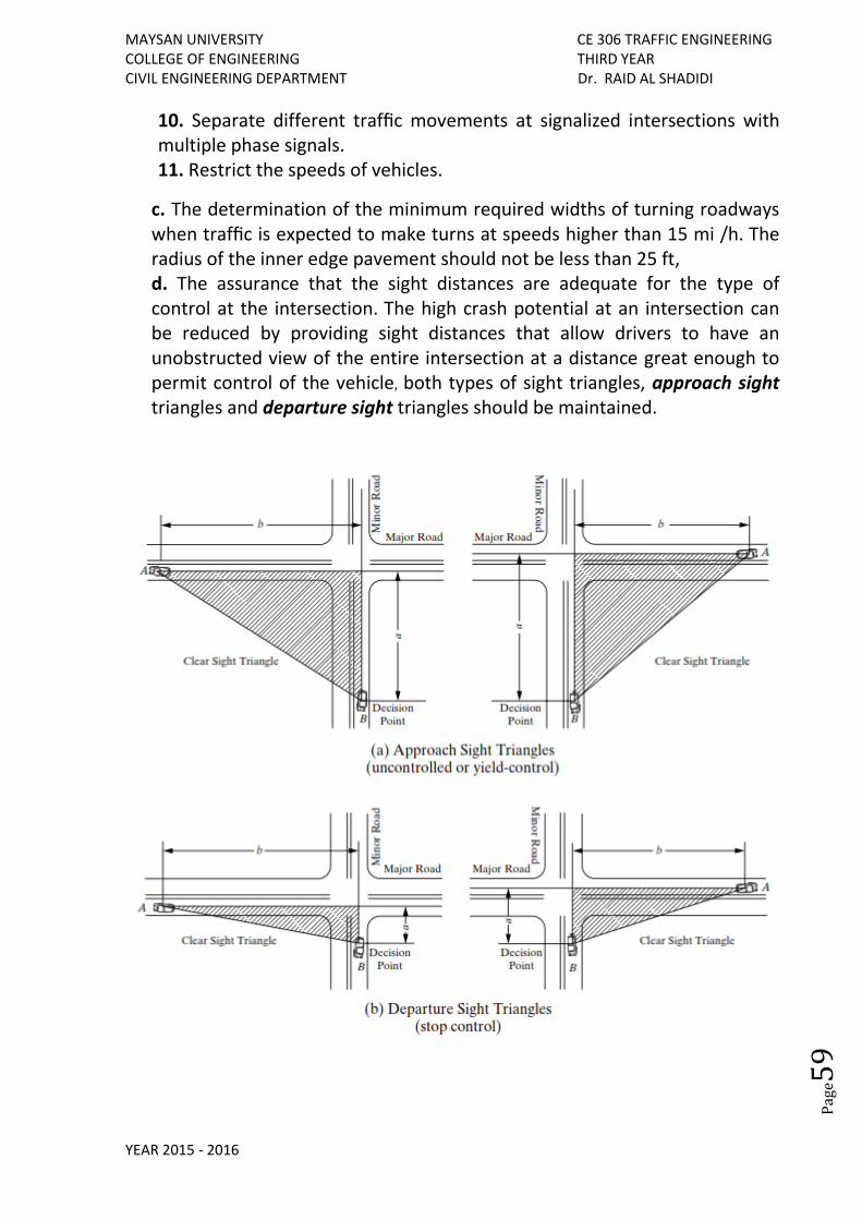
c. The determination of the minimum required widths of turning roadways when traffic is expected to make turns at speeds higher than 15 mi /h. The radius of the inner edge pavement should not be less than 25 ft, d. The assurance that the sight distances are adequate for the type of control at the intersection. The high crash potential at an intersection can be reduced by providing sight distances that allow drivers to have an unobstructed view of the entire intersection at a distance great enough to permit control of the vehicle, both types of sight triangles, approach sight triangles and departure sight triangles should be maintained.
MAYSAN UNIVERSITY CE 306 TRAFFIC ENGINEERING COLLEGE OF ENGINEERING THIRD YEAR CIVIL ENGINEERING DEPARTMENT Dr. RAID AL SHADIDI
YEAR 2015 - 2016
Pag
e60
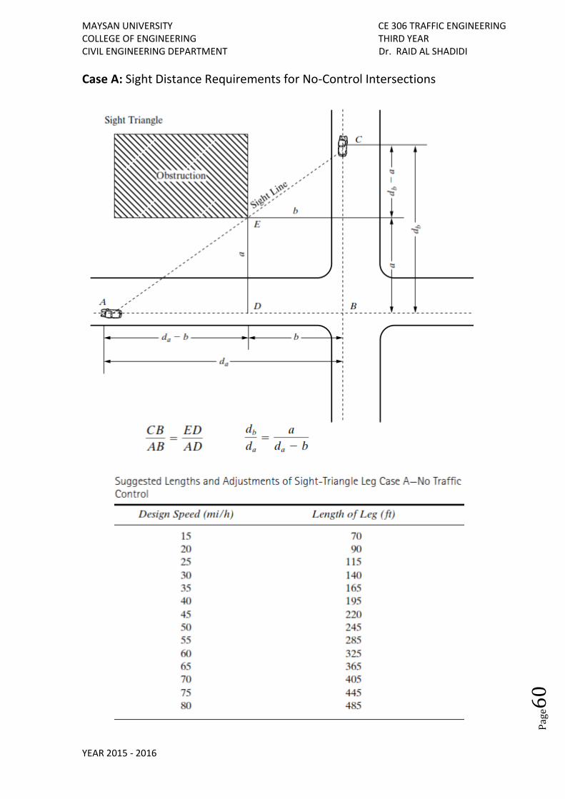
Case A: Sight Distance Requirements for No-Control Intersections
MAYSAN UNIVERSITY CE 306 TRAFFIC ENGINEERING COLLEGE OF ENGINEERING THIRD YEAR CIVIL ENGINEERING DEPARTMENT Dr. RAID AL SHADIDI
YEAR 2015 - 2016
Pag
e61
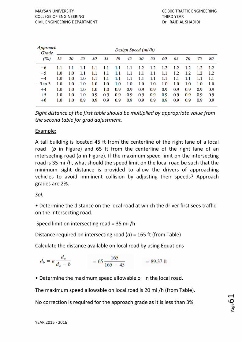
Sight distance of the first table should be multiplied by appropriate value from the second table for grad adjustment.
Example:
A tall building is located 45 ft from the centerline of the right lane of a local road (b in Figure) and 65 ft from the centerline of the right lane of an intersecting road (a in Figure). If the maximum speed limit on the intersecting road is 35 mi /h, what should the speed limit on the local road be such that the minimum sight distance is provided to allow the drivers of approaching vehicles to avoid imminent collision by adjusting their speeds? Approach grades are 2%.
Sol.
• Determine the distance on the local road at which the driver first sees traffic on the intersecting road.
Speed limit on intersecting road = 35 mi /h
Distance required on intersecting road (d) = 165 ft (from Table)
Calculate the distance available on local road by using Equations
• Determine the maximum speed allowable o n the local road.
The maximum speed allowable on local road is 20 mi /h (from Table).
No correction is required for the approach grade as it is less than 3%.
MAYSAN UNIVERSITY CE 306 TRAFFIC ENGINEERING COLLEGE OF ENGINEERING THIRD YEAR CIVIL ENGINEERING DEPARTMENT Dr. RAID AL SHADIDI
YEAR 2015 - 2016
Pag
e62
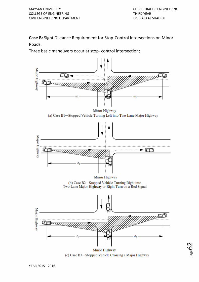
Case B: Sight Distance Requirement for Stop-Control Intersections on Minor
Roads.
Three basic maneuvers occur at stop- control intersection;
MAYSAN UNIVERSITY CE 306 TRAFFIC ENGINEERING COLLEGE OF ENGINEERING THIRD YEAR CIVIL ENGINEERING DEPARTMENT Dr. RAID AL SHADIDI
YEAR 2015 - 2016
Pag
e63
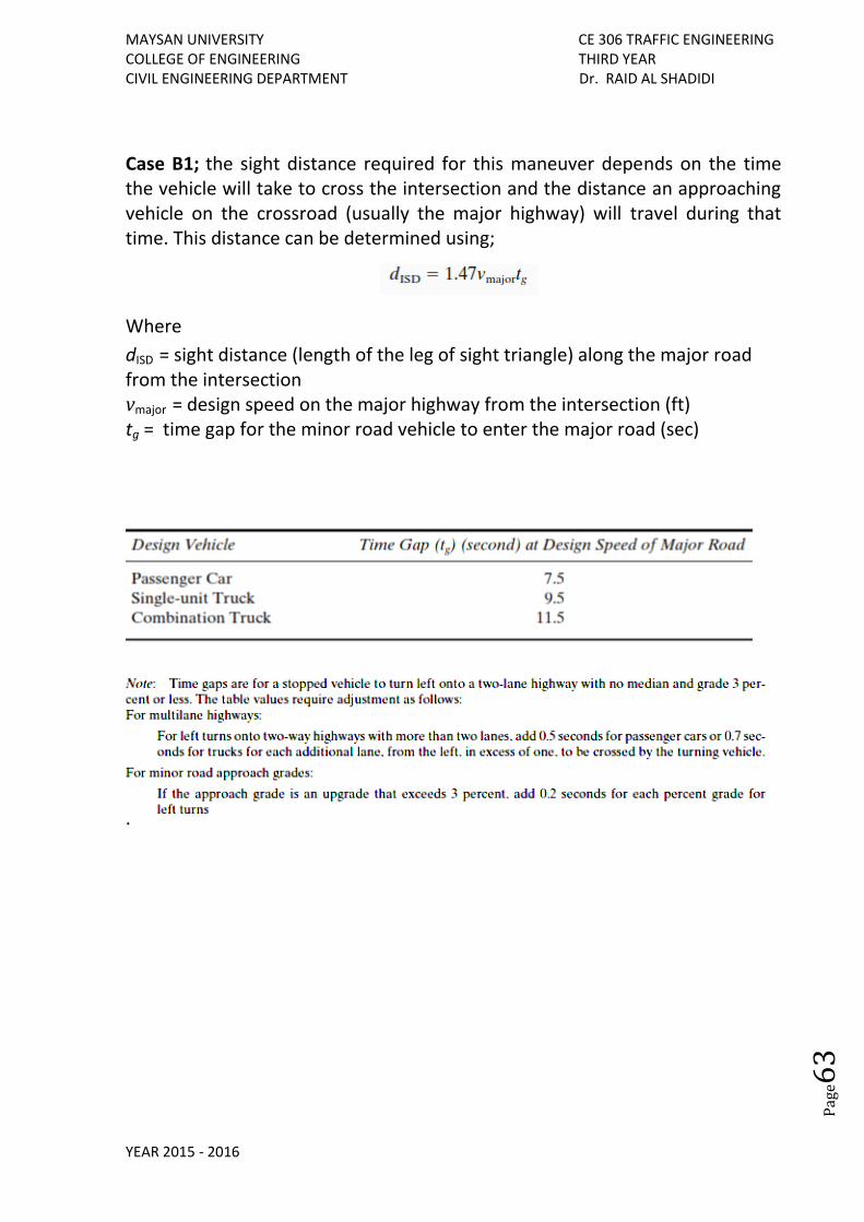
Case B1; the sight distance required for this maneuver depends on the time the vehicle will take to cross the intersection and the distance an approaching vehicle on the crossroad (usually the major highway) will travel during that time. This distance can be determined using;
Where
dISD = sight distance (length of the leg of sight triangle) along the major road from the intersection vmajor = design speed on the major highway from the intersection (ft) tg = time gap for the minor road vehicle to enter the major road (sec)
.
MAYSAN UNIVERSITY CE 306 TRAFFIC ENGINEERING COLLEGE OF ENGINEERING THIRD YEAR CIVIL ENGINEERING DEPARTMENT Dr. RAID AL SHADIDI
YEAR 2015 - 2016
Pag
e64
Example: A minor road intersects a major four-lane undivided road with a design speed of 65 mi /h. The intersection is controlled with a stop sign on the minor road. If the design vehicle is a single-unit truck, determine the minimum sight distance required on the major road that will allow a stopped vehicle on the minor road to safely turn left if the approach grade on the minor road is 2%. Sol.
From Table, tg = 9.5 sec (for a single unit truck) Correct for number of lanes : tg =(9.5 + 0.7) sec =10.2 sec (Note no adjustment is necessary for approach grade as it is not higher than 3%.)
• Determine minimum sight distance = 1.47 x 65 x 10.2 = 974.61 ft.
Example:
A minor road intersects a major four-lane divided road with a design speed of 65 mi /h and a median width of 6 ft. The intersection is controlled with a stop sign on the minor road. If the design vehicle is a passenger car, determine the minimum sight distance required on the major road for the stopped vehicle to turn left onto the major road if the approach grade on the minor road is 4%.
Sol.
From Table, tg = 7.5 sec (for a passenger car)
Correct for number of lanes: tg= (7.5 + 0.5 x 1.5) sec = 8.25 sec
(This assumes that the 6 ft median is equivalent to half a lane.)
Correct for approach grade tg = (8.25 + 0.2 x 1) sec = 8.45 sec
(Grade is 1% higher than 3%.)
• Determine minimum sight distance = 1.47 x 65 x 8.45 = 810 ft.
MAYSAN UNIVERSITY CE 306 TRAFFIC ENGINEERING COLLEGE OF ENGINEERING THIRD YEAR CIVIL ENGINEERING DEPARTMENT Dr. RAID AL SHADIDI
YEAR 2015 - 2016
Pag
e65
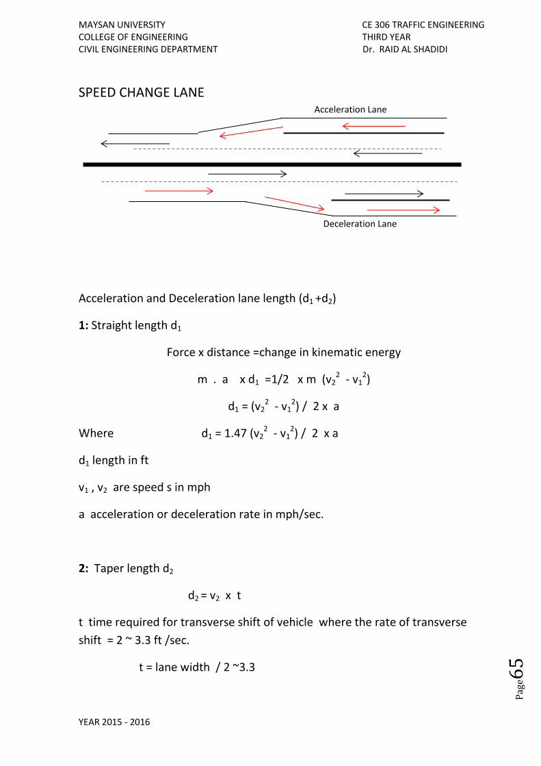
SPEED CHANGE LANE
Acceleration and Deceleration lane length (d1 +d2)
1: Straight length d1
Force x distance =change in kinematic energy
m . a x d1 =1/2 x m (v22 - v1
2)
d1 = (v22 - v1
2) / 2 x a
Where d1 = 1.47 (v22 - v1
2) / 2 x a
d1 length in ft
v1 , v2 are speed s in mph
a acceleration or deceleration rate in mph/sec.
2: Taper length d2
d2 = v2 x t
t time required for transverse shift of vehicle where the rate of transverse
shift = 2 ~ 3.3 ft /sec.
t = lane width / 2 ~3.3
Deceleration Lane
Acceleration Lane
MAYSAN UNIVERSITY CE 306 TRAFFIC ENGINEERING COLLEGE OF ENGINEERING THIRD YEAR CIVIL ENGINEERING DEPARTMENT Dr. RAID AL SHADIDI
YEAR 2015 - 2016
Pag
e66
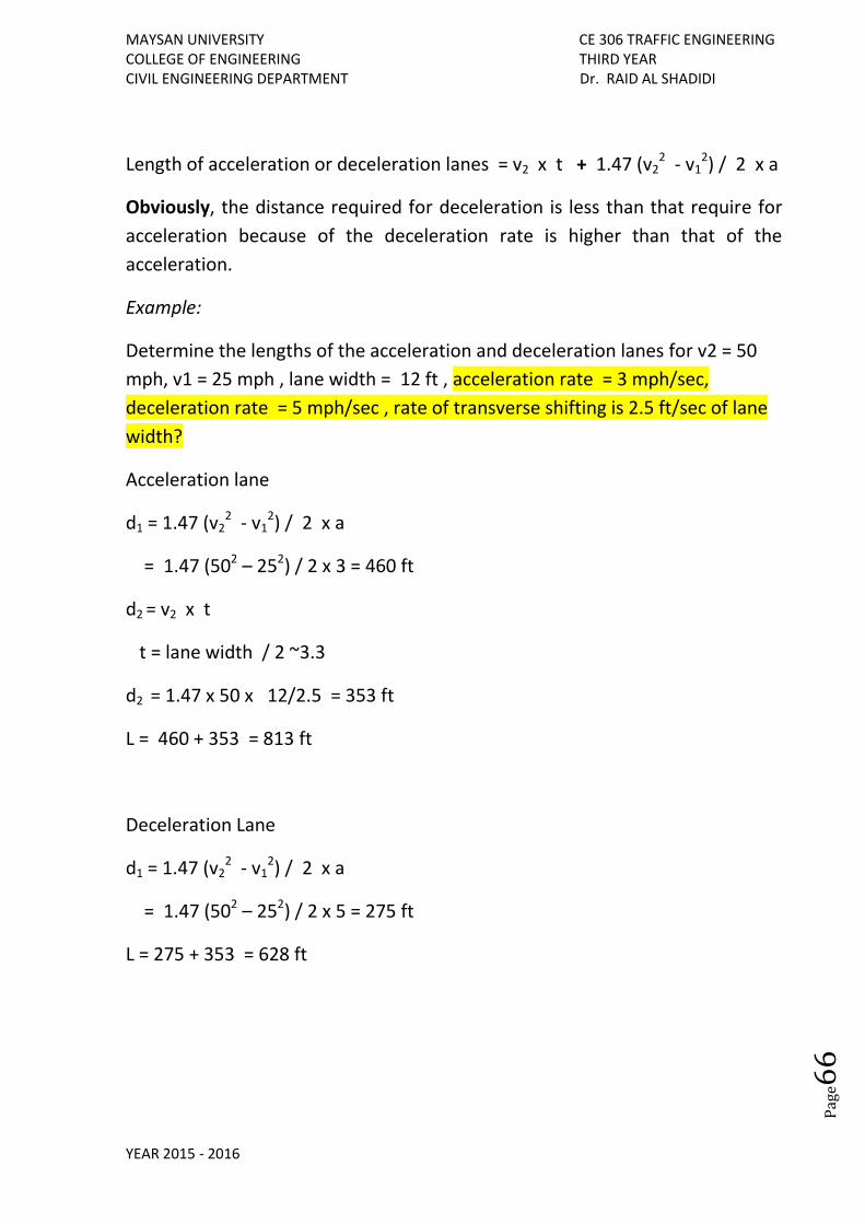
Length of acceleration or deceleration lanes = v2 x t + 1.47 (v22 - v1
2) / 2 x a
Obviously, the distance required for deceleration is less than that require for
acceleration because of the deceleration rate is higher than that of the
acceleration.
Example:
Determine the lengths of the acceleration and deceleration lanes for v2 = 50
mph, v1 = 25 mph , lane width = 12 ft , acceleration rate = 3 mph/sec,
deceleration rate = 5 mph/sec , rate of transverse shifting is 2.5 ft/sec of lane
width?
Acceleration lane
d1 = 1.47 (v22 - v1
2) / 2 x a
= 1.47 (502 – 252) / 2 x 3 = 460 ft
d2 = v2 x t
t = lane width / 2 ~3.3
d2 = 1.47 x 50 x 12/2.5 = 353 ft
L = 460 + 353 = 813 ft
Deceleration Lane
d1 = 1.47 (v22 - v1
2) / 2 x a
= 1.47 (502 – 252) / 2 x 5 = 275 ft
L = 275 + 353 = 628 ft
MAYSAN UNIVERSITY CE 306 TRAFFIC ENGINEERING COLLEGE OF ENGINEERING THIRD YEAR CIVIL ENGINEERING DEPARTMENT Dr. RAID AL SHADIDI
YEAR 2015 - 2016
Pag
e67
Case B2; (tg) are adjusted in consideration of the fact that drivers tend to
accept gaps that are slightly lower than those for left turns. AASHTO suggests
that values shown on table should be decreased by 1 second. In cases where
this sight distance is not available, reducing the speed limit on the major road.
Case B3: Minimum requirements determined for right and left turns as presented for Cases B1 and B2 will usually satisfy the requirements for the crossing maneuver. AASHTO, however, recommends that the available sight distance for crossing be checked when the following conditions exist: • When only a crossing maneuver is allowed at the intersection, • When the crossing maneuver will involve an equivalent width of more than six lanes, or • Where the vehicle mix of the crossing traffic includes a substantial number of heavy vehicles and the existence of steep grades that may slow down these heavy vehicles while their back portion is still in the intersection.
MAYSAN UNIVERSITY CE 306 TRAFFIC ENGINEERING COLLEGE OF ENGINEERING THIRD YEAR CIVIL ENGINEERING DEPARTMENT Dr. RAID AL SHADIDI
YEAR 2015 - 2016
Pag
e68
INTERSECTION CONTROL
An intersection is an area shared by two or more roads. Its main function is
to allow the change of route directions. It is necessary gives a brief description
to facilitate a clear understanding of the elements of intersection control. The
intersection is therefore an area of decision for all drivers; each must select
one of the available choices to proceed. This requires an additional effort by
the driver that is not necessary in non-intersection areas of a highway. The
flow of traffic on any street or highway is greatly affected by the flow of traffic
through the intersection points on that street or highway because the
intersection usually performs at a level below that of any other section of the
road. Several types of traffic-control systems are used to reduce traffic delays
and crashes on at-grade intersections and to increase the capacity of highways
and streets. However, appropriate regulations must be enforced if these
systems are to be effective.
General Concepts of Traffic Control
The purpose of traffic control is to assign the right of way to drivers and thus to
facilitate highway safety by ensuring the orderly and predictable movement of
all traffic on highways. Control may be achieved by using traffic signals, signs,
or markings that regulate, guide, warn, and/or channel traffic. The more
complex the maneuvering area, the greater the need for a properly designed
traffic-control system. Many intersections are complex maneuvering areas and
therefore require properly designed traffic-control systems. Guidelines for
determining whether a particular control type is suitable for a given
intersection are provided in the Manual on Uniform Traffic Control Devices
(MUTCD). To be effective, a traffic-control device must:
• Fulfill a need
• Command attention
• Convey a clear, simple meaning
• Command the respect of road users
MAYSAN UNIVERSITY CE 306 TRAFFIC ENGINEERING COLLEGE OF ENGINEERING THIRD YEAR CIVIL ENGINEERING DEPARTMENT Dr. RAID AL SHADIDI
YEAR 2015 - 2016
Pag
e69
• Give adequate time for proper response
To ensure that a traffic-control device possesses these five properties, the
MUTCD recommends that engineers consider the following five factors:
1. Design. The device should be designed with a combination of size, color, and shape that will convey a message and command the respect and attention of the driver. 2. Placement. The device should be located so that it is within the cone of vision of the viewer and the driver has adequate response time when driving at normal speed. 3. Operation. The device should be used in a manner that ensures the fulfillment of traffic requirements in a consistent and uniform way. 4. Maintenance. The device must be regularly maintained to ensure that legibility is sustained. 5. Uniformity. To facilitate the recognition and understanding of these devices by drivers, similar devices should be used at locations with similar traffic and geometric characteristics. In addition to these considerations, it is essential that engineers avoid using control devices that conflict with one another at the same location. It is imperative that control devices aid each other in transmitting the required message to the driver. Conflict Points at Intersections
Conflicts occur when traffic streams moving in different directions interfere
with each other. The three types of conflicts are merging, diverging, and
crossing. Figure shows the different conflict points that exist at a four-
approach unsignalized intersection. There are 32 conflict points in this case.
The number of possible conflict points at any intersection depends on the
number of approaches, the turning movements, and the type of traffic control
at the intersection. The primary objective in the design of a traffic-control
system at an intersection is to reduce the number of significant conflict points.
In designing such a system, it is first necessary to undertake an analysis of the
turning movements at the intersection which will indicate the significant types
of conflicts. Factors that influence the significance of a conflict include the type
of conflict, the number of vehicles in each conflicting stream, and the speeds of
the vehicles in those streams. Crossing conflicts, however, tend to have the
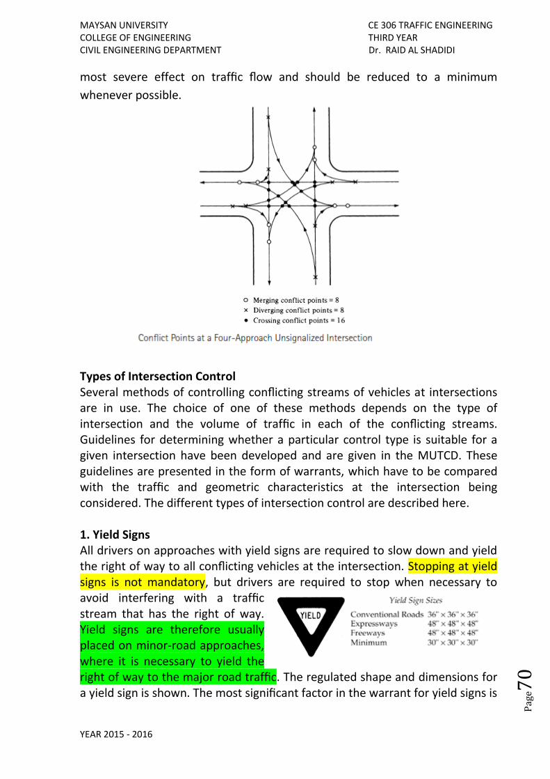
MAYSAN UNIVERSITY CE 306 TRAFFIC ENGINEERING COLLEGE OF ENGINEERING THIRD YEAR CIVIL ENGINEERING DEPARTMENT Dr. RAID AL SHADIDI
YEAR 2015 - 2016
Pag
e70
most severe effect on traffic flow and should be reduced to a minimum
whenever possible.
Types of Intersection Control Several methods of controlling conflicting streams of vehicles at intersections are in use. The choice of one of these methods depends on the type of intersection and the volume of traffic in each of the conflicting streams. Guidelines for determining whether a particular control type is suitable for a given intersection have been developed and are given in the MUTCD. These guidelines are presented in the form of warrants, which have to be compared with the traffic and geometric characteristics at the intersection being considered. The different types of intersection control are described here. 1. Yield Signs All drivers on approaches with yield signs are required to slow down and yield the right of way to all conflicting vehicles at the intersection. Stopping at yield signs is not mandatory, but drivers are required to stop when necessary to avoid interfering with a traffic stream that has the right of way. Yield signs are therefore usually placed on minor-road approaches, where it is necessary to yield the right of way to the major road traffic. The regulated shape and dimensions for a yield sign is shown. The most significant factor in the warrant for yield signs is
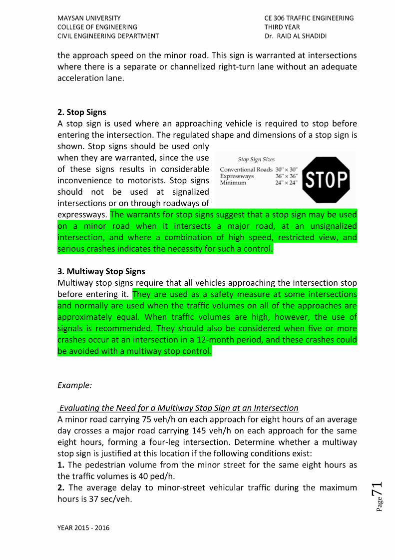
MAYSAN UNIVERSITY CE 306 TRAFFIC ENGINEERING COLLEGE OF ENGINEERING THIRD YEAR CIVIL ENGINEERING DEPARTMENT Dr. RAID AL SHADIDI
YEAR 2015 - 2016
Pag
e71
the approach speed on the minor road. This sign is warranted at intersections where there is a separate or channelized right-turn lane without an adequate acceleration lane. 2. Stop Signs A stop sign is used where an approaching vehicle is required to stop before entering the intersection. The regulated shape and dimensions of a stop sign is shown. Stop signs should be used only when they are warranted, since the use of these signs results in considerable inconvenience to motorists. Stop signs should not be used at signalized intersections or on through roadways of expressways. The warrants for stop signs suggest that a stop sign may be used on a minor road when it intersects a major road, at an unsignalized intersection, and where a combination of high speed, restricted view, and serious crashes indicates the necessity for such a control. 3. Multiway Stop Signs Multiway stop signs require that all vehicles approaching the intersection stop before entering it. They are used as a safety measure at some intersections and normally are used when the traffic volumes on all of the approaches are approximately equal. When traffic volumes are high, however, the use of signals is recommended. They should also be considered when five or more crashes occur at an intersection in a 12-month period, and these crashes could be avoided with a multiway stop control. Example: Evaluating the Need for a Multiway Stop Sign at an Intersection A minor road carrying 75 veh/h on each approach for eight hours of an average day crosses a major road carrying 145 veh/h on each approach for the same eight hours, forming a four-leg intersection. Determine whether a multiway stop sign is justified at this location if the following conditions exist: 1. The pedestrian volume from the minor street for the same eight hours as the traffic volumes is 40 ped/h. 2. The average delay to minor-street vehicular traffic during the maximum hours is 37 sec/veh.
MAYSAN UNIVERSITY CE 306 TRAFFIC ENGINEERING COLLEGE OF ENGINEERING THIRD YEAR CIVIL ENGINEERING DEPARTMENT Dr. RAID AL SHADIDI
YEAR 2015 - 2016
Pag
e72
3. There are an average of four crashes per year that may be corrected by a multiway stop control. Sol. . Determine whether traffic volume on the major street satisfies the warrant. Total vehicular volume entering the intersection from the major approaches is 145 + 145 = 290 veh/h. The major road traffic volume criterion is not satisfied. The volume warrants for this control specify that the total volume on both major street approaches should not be less than 300 veh/h for any eight hours of an average day. . Determine whether total minor-road traffic and pedestrian volume satisfies the warrant. Total minor-road traffic and pedestrian volume = 2 x 75 + 40 =190. Total minor-road and pedestrian volume is not satisfied. The combined volume warrant of vehicles and pedestrians from the minor approaches should not be less than 200 units/h for the same eight hours. . Determine whether crash criterion is satisfied.Total number of crashes per year = 4. Crash criterion is not satisfied. Five or more crashes occur at an intersection in a 12-month period, and these crashes could be avoided with a multiway stop control. .However, each crash and volume criterion is satisfied up to 80% of the minimum required. If each of volume and safety warrant satisfies 80 percent of the minimum requirement, the installation of a multiway stop sign is justified. The installation of a multiway stop control is justified. 4. Intersection Channelization Intersection channelization is used mainly to separate turn lanes from through lanes. A channelized intersection consists of solid white lines or raised barriers which guide traffic within a lane so that vehicles can safely negotiate a complex intersection. When raised islands are used, they can also provide a refuge for pedestrians. Design Guide. Guidelines for the use of channels at intersections include:
MAYSAN UNIVERSITY CE 306 TRAFFIC ENGINEERING COLLEGE OF ENGINEERING THIRD YEAR CIVIL ENGINEERING DEPARTMENT Dr. RAID AL SHADIDI
YEAR 2015 - 2016
Pag
e73
• Laying out islands or channel lines to allow a natural, convenient flow of traffic • Avoiding confusion by using a few well-located islands • Providing adequate radii of curves and widths of lanes for the prevailing type of vehicle 5. Traffic Signals One of the most effective ways of controlling traffic at an intersection is the use of traffic signals. Traffic signals can be used to eliminate many conflicts because different traffic streams can be assigned the use of the intersection at different times. Since this results in a delay to vehicles in all streams, it is important that traffic signals be used only when necessary. The most important factor that determines the need for traffic signals at a particular intersection is the intersection’s approach traffic volume, although other factors such as pedestrian volume and crash experience may also play a significant role. The Manual on Traffic Signal Design gives the fundamental concepts and standard practices used in the design of traffic signals. In addition, the MUTCD describes eight warrants in detail, at least one of which should be satisfied for an intersection to be signalized. However, these warrants should be considered only as a guide; professional judgment based on experience also should be used to decide whether or not an intersection should be signalized. The factors considered in the warrants are: • Warrant 1, Eight-hour vehicular volume • Warrant 2, Four-hour vehicular volume • Warrant 3, Peak hour • Warrant 4, Pedestrian volume • Warrant 5, School crossing • Warrant 6, Coordinated signal system • Warrant 7, Crash experience • Warrant 8, Roadway network Example:
Determining Whether the Conditions at an Intersection Warrant Installing a Traffic-Signal Control? A two-lane minor street crosses a four-lane major street. If the traffic conditions are as given, determine whether installing a traffic signal at this intersection is warranted?
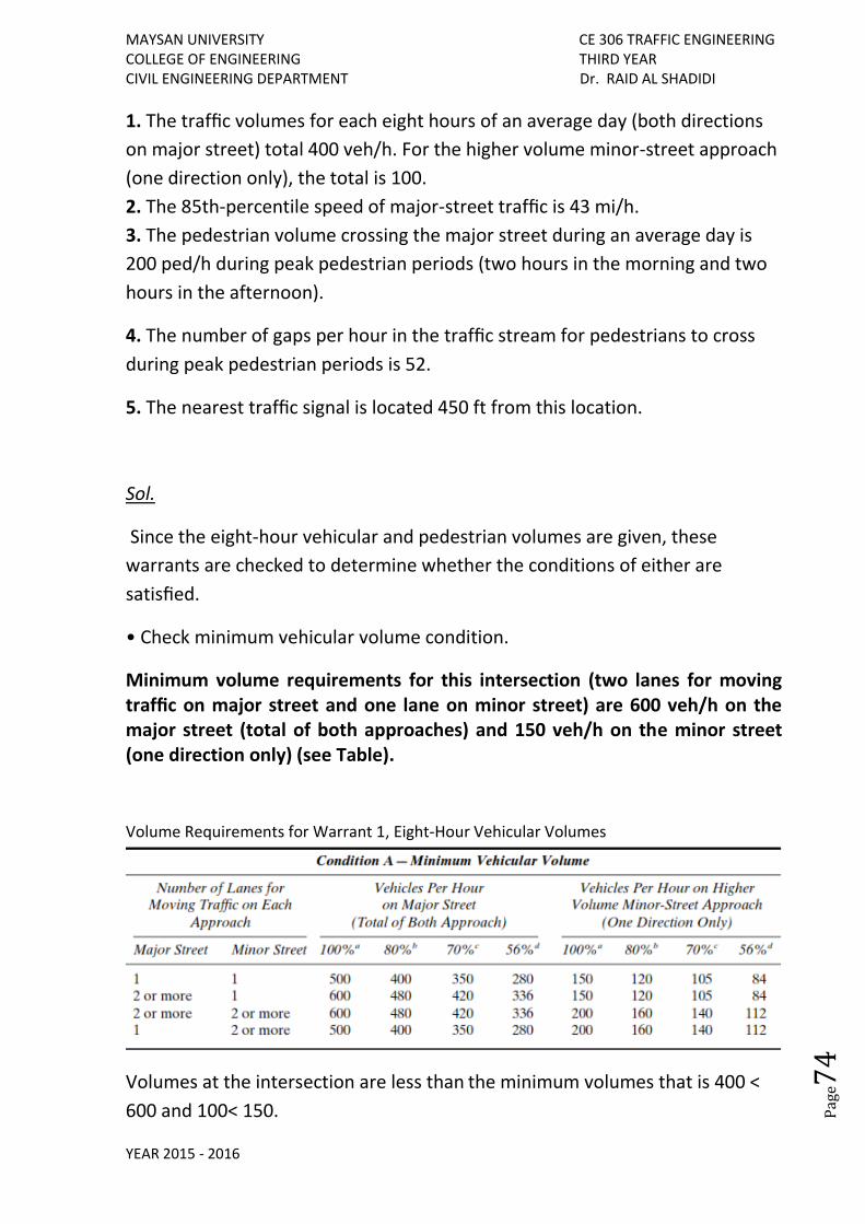
MAYSAN UNIVERSITY CE 306 TRAFFIC ENGINEERING COLLEGE OF ENGINEERING THIRD YEAR CIVIL ENGINEERING DEPARTMENT Dr. RAID AL SHADIDI
YEAR 2015 - 2016
Pag
e74
1. The traffic volumes for each eight hours of an average day (both directions
on major street) total 400 veh/h. For the higher volume minor-street approach
(one direction only), the total is 100.
2. The 85th-percentile speed of major-street traffic is 43 mi/h.
3. The pedestrian volume crossing the major street during an average day is
200 ped/h during peak pedestrian periods (two hours in the morning and two
hours in the afternoon).
4. The number of gaps per hour in the traffic stream for pedestrians to cross
during peak pedestrian periods is 52.
5. The nearest traffic signal is located 450 ft from this location.
Sol.
Since the eight-hour vehicular and pedestrian volumes are given, these
warrants are checked to determine whether the conditions of either are
satisfied.
• Check minimum vehicular volume condition.
Minimum volume requirements for this intersection (two lanes for moving traffic on major street and one lane on minor street) are 600 veh/h on the major street (total of both approaches) and 150 veh/h on the minor street
(one direction only) (see Table).
Volume Requirements for Warrant 1, Eight-Hour Vehicular Volumes
Volumes at the intersection are less than the minimum volumes that is 400 ˂
600 and 100˂ 150.
MAYSAN UNIVERSITY CE 306 TRAFFIC ENGINEERING COLLEGE OF ENGINEERING THIRD YEAR CIVIL ENGINEERING DEPARTMENT Dr. RAID AL SHADIDI
YEAR 2015 - 2016
Pag
e75
However, because the 85th-percentile speed is 43 mi/h ˃ 40 mi/h, the minimum volumes required can be reduced to 70 percent of the requirements. Therefore, minimum required volumes are 600 x 0.7 = 420 and 150 x 0.7 = 105
The volumes at the intersection are still less than the adjusted required volumes. The minimum vehicular volumes warrant therefore is not satisfied.
• Check minimum pedestrian volume.
The minimum pedestrian volumes required are 100 or more for each of any four hours or 190 or more during any hour.
With 200 pedestrians/hr during the peak pedestrian volumes, the minimum
requirement for pedestrian volumes is satisfied.
• Check minimum number of acceptable gaps.
The maximum acceptable gaps for pedestrian crossing are 60 gaps/hr. The number of gaps available is 52. The number of gaps for pedestrian crossing is Insufficient and the acceptable-gaps condition is satisfied.
• Check location of nearest traffic signal.
For the location of the nearest traffic signal along the major street, the minimum distance required is 300 ft. The nearest traffic signal to the intersection is 450 ft away; 450 ˃300. Thus, the location of the nearest traffic signal condition is satisfied.
A traffic signal therefore is justified under the minimum pedestrian volume warrant. The signal should be of the traffic-actuated type with pushbuttons for pedestrians who are crossing.
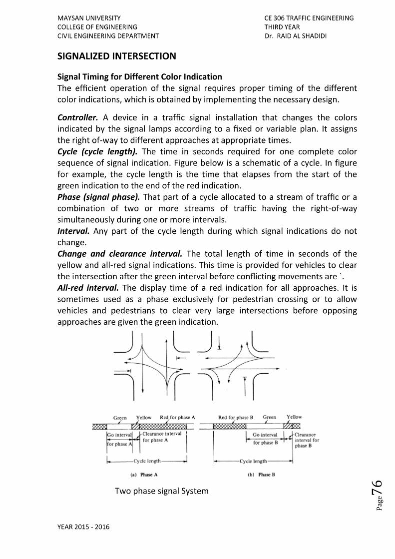
MAYSAN UNIVERSITY CE 306 TRAFFIC ENGINEERING COLLEGE OF ENGINEERING THIRD YEAR CIVIL ENGINEERING DEPARTMENT Dr. RAID AL SHADIDI
YEAR 2015 - 2016
Pag
e76
SIGNALIZED INTERSECTION
Signal Timing for Different Color Indication The efficient operation of the signal requires proper timing of the different color indications, which is obtained by implementing the necessary design.
Controller. A device in a traffic signal installation that changes the colors indicated by the signal lamps according to a fixed or variable plan. It assigns the right of-way to different approaches at appropriate times. Cycle (cycle length). The time in seconds required for one complete color sequence of signal indication. Figure below is a schematic of a cycle. In figure for example, the cycle length is the time that elapses from the start of the green indication to the end of the red indication. Phase (signal phase). That part of a cycle allocated to a stream of traffic or a combination of two or more streams of traffic having the right-of-way simultaneously during one or more intervals. Interval. Any part of the cycle length during which signal indications do not change. Change and clearance interval. The total length of time in seconds of the yellow and all-red signal indications. This time is provided for vehicles to clear the intersection after the green interval before conflicting movements are `. All-red interval. The display time of a red indication for all approaches. It is sometimes used as a phase exclusively for pedestrian crossing or to allow vehicles and pedestrians to clear very large intersections before opposing approaches are given the green indication.
Two phase signal System
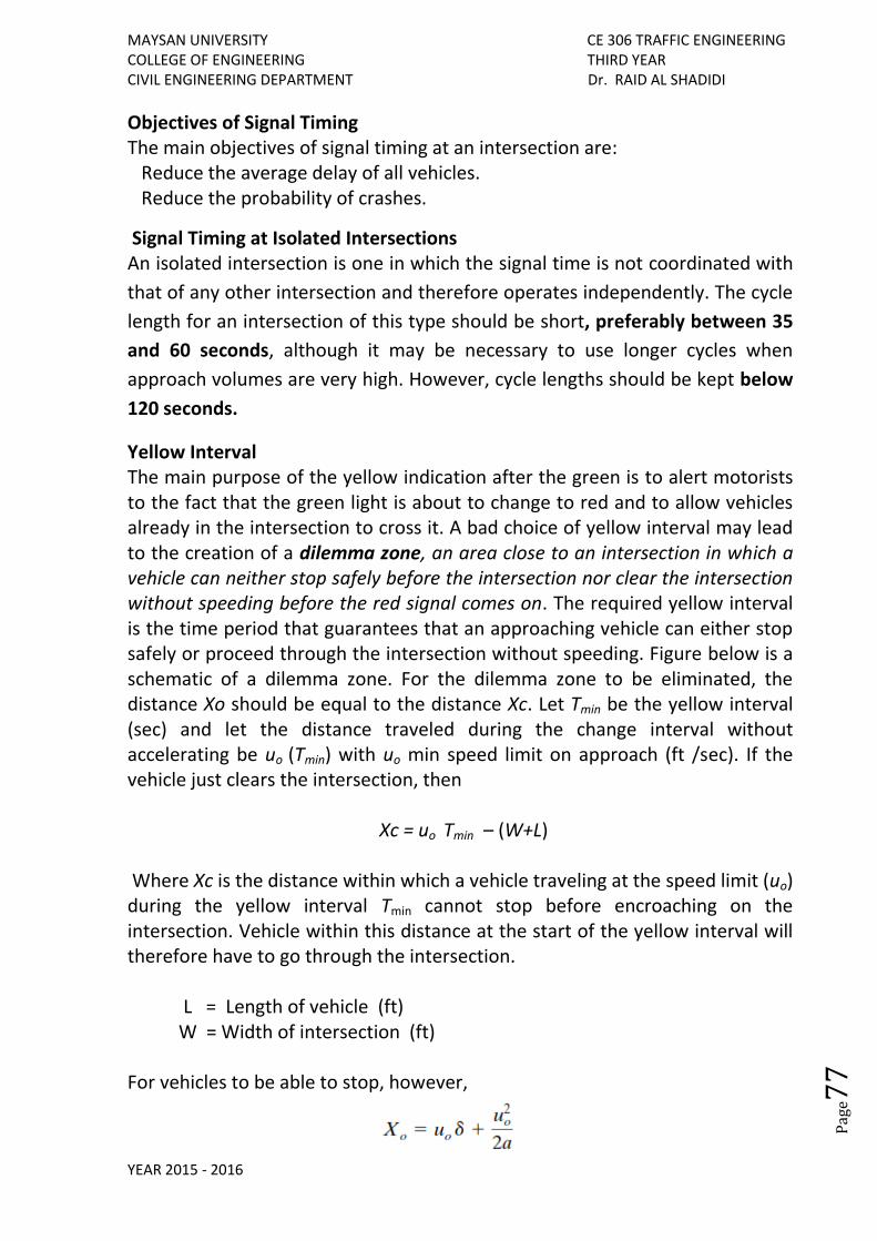
MAYSAN UNIVERSITY CE 306 TRAFFIC ENGINEERING COLLEGE OF ENGINEERING THIRD YEAR CIVIL ENGINEERING DEPARTMENT Dr. RAID AL SHADIDI
YEAR 2015 - 2016
Pag
e77
Objectives of Signal Timing The main objectives of signal timing at an intersection are: Reduce the average delay of all vehicles. Reduce the probability of crashes.
Signal Timing at Isolated Intersections An isolated intersection is one in which the signal time is not coordinated with
that of any other intersection and therefore operates independently. The cycle
length for an intersection of this type should be short, preferably between 35
and 60 seconds, although it may be necessary to use longer cycles when
approach volumes are very high. However, cycle lengths should be kept below
120 seconds.
Yellow Interval The main purpose of the yellow indication after the green is to alert motorists to the fact that the green light is about to change to red and to allow vehicles already in the intersection to cross it. A bad choice of yellow interval may lead to the creation of a dilemma zone, an area close to an intersection in which a vehicle can neither stop safely before the intersection nor clear the intersection without speeding before the red signal comes on. The required yellow interval is the time period that guarantees that an approaching vehicle can either stop safely or proceed through the intersection without speeding. Figure below is a schematic of a dilemma zone. For the dilemma zone to be eliminated, the distance Xo should be equal to the distance Xc. Let Tmin be the yellow interval (sec) and let the distance traveled during the change interval without accelerating be uo (Tmin) with uo min speed limit on approach (ft /sec). If the vehicle just clears the intersection, then Xc = uo Tmin – (W+L) Where Xc is the distance within which a vehicle traveling at the speed limit (uo) during the yellow interval Tmin cannot stop before encroaching on the intersection. Vehicle within this distance at the start of the yellow interval will therefore have to go through the intersection. L = Length of vehicle (ft) W = Width of intersection (ft) For vehicles to be able to stop, however,
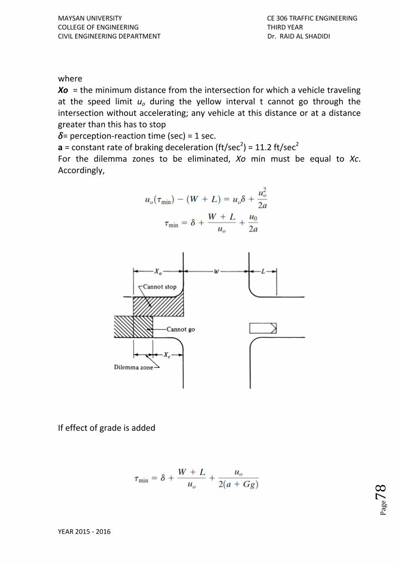
MAYSAN UNIVERSITY CE 306 TRAFFIC ENGINEERING COLLEGE OF ENGINEERING THIRD YEAR CIVIL ENGINEERING DEPARTMENT Dr. RAID AL SHADIDI
YEAR 2015 - 2016
Pag
e78
where Xo = the minimum distance from the intersection for which a vehicle traveling at the speed limit uo during the yellow interval t cannot go through the intersection without accelerating; any vehicle at this distance or at a distance greater than this has to stop 𝛿= perception-reaction time (sec) = 1 sec. a = constant rate of braking deceleration (ft/sec2) = 11.2 ft/sec2 For the dilemma zones to be eliminated, Xo min must be equal to Xc. Accordingly,
If effect of grade is added
MAYSAN UNIVERSITY CE 306 TRAFFIC ENGINEERING COLLEGE OF ENGINEERING THIRD YEAR CIVIL ENGINEERING DEPARTMENT Dr. RAID AL SHADIDI
YEAR 2015 - 2016
Pag
e79
Safety considerations, however, normally preclude yellow intervals of less than three seconds and to encourage motorists’ respect for the yellow interval, it is usually not made longer than five seconds. Determining the Minimum Yellow Interval at an Intersection Example: Determine the minimum yellow interval at an intersection whose width is 40 ft if the maximum allowable speed on the approach roads is 30 mi/h. Assume average length of vehicle is 20 ft. Sol: We must first decide on a deceleration rate. AASHTO recommends a deceleration rate of 11.2 ft /sec2. Assuming this value for a and taking 𝛿 as 1.0 sec, we obtain
In this case, a yellow period of 4.5 sec will be needed.
Cycle Lengths of Fixed (Pretimed) Signals (Webstar method)
By using the equation below minimum intersection delay can be achieved.
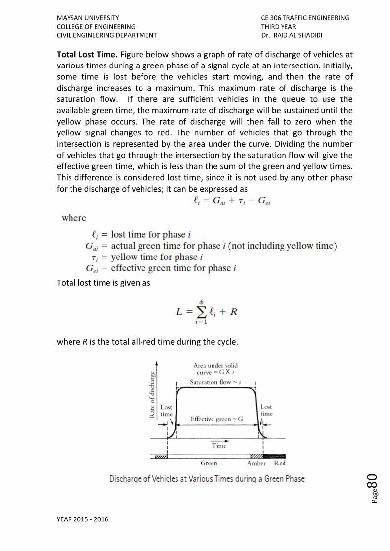
MAYSAN UNIVERSITY CE 306 TRAFFIC ENGINEERING COLLEGE OF ENGINEERING THIRD YEAR CIVIL ENGINEERING DEPARTMENT Dr. RAID AL SHADIDI
YEAR 2015 - 2016
Pag
e80
Total Lost Time. Figure below shows a graph of rate of discharge of vehicles at various times during a green phase of a signal cycle at an intersection. Initially, some time is lost before the vehicles start moving, and then the rate of discharge increases to a maximum. This maximum rate of discharge is the saturation flow. If there are sufficient vehicles in the queue to use the available green time, the maximum rate of discharge will be sustained until the yellow phase occurs. The rate of discharge will then fall to zero when the yellow signal changes to red. The number of vehicles that go through the intersection is represented by the area under the curve. Dividing the number of vehicles that go through the intersection by the saturation flow will give the effective green time, which is less than the sum of the green and yellow times. This difference is considered lost time, since it is not used by any other phase for the discharge of vehicles; it can be expressed as
Total lost time is given as
where R is the total all-red time during the cycle.
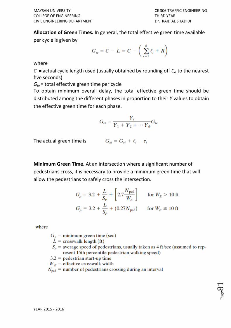
MAYSAN UNIVERSITY CE 306 TRAFFIC ENGINEERING COLLEGE OF ENGINEERING THIRD YEAR CIVIL ENGINEERING DEPARTMENT Dr. RAID AL SHADIDI
YEAR 2015 - 2016
Pag
e81
Allocation of Green Times. In general, the total effective green time available
per cycle is given by
where
C = actual cycle length used (usually obtained by rounding off Co to the nearest five seconds) Gte = total effective green time per cycle
To obtain minimum overall delay, the total effective green time should be
distributed among the different phases in proportion to their Y values to obtain
the effective green time for each phase.
The actual green time is
Minimum Green Time. At an intersection where a significant number of
pedestrians cross, it is necessary to provide a minimum green time that will
allow the pedestrians to safely cross the intersection.
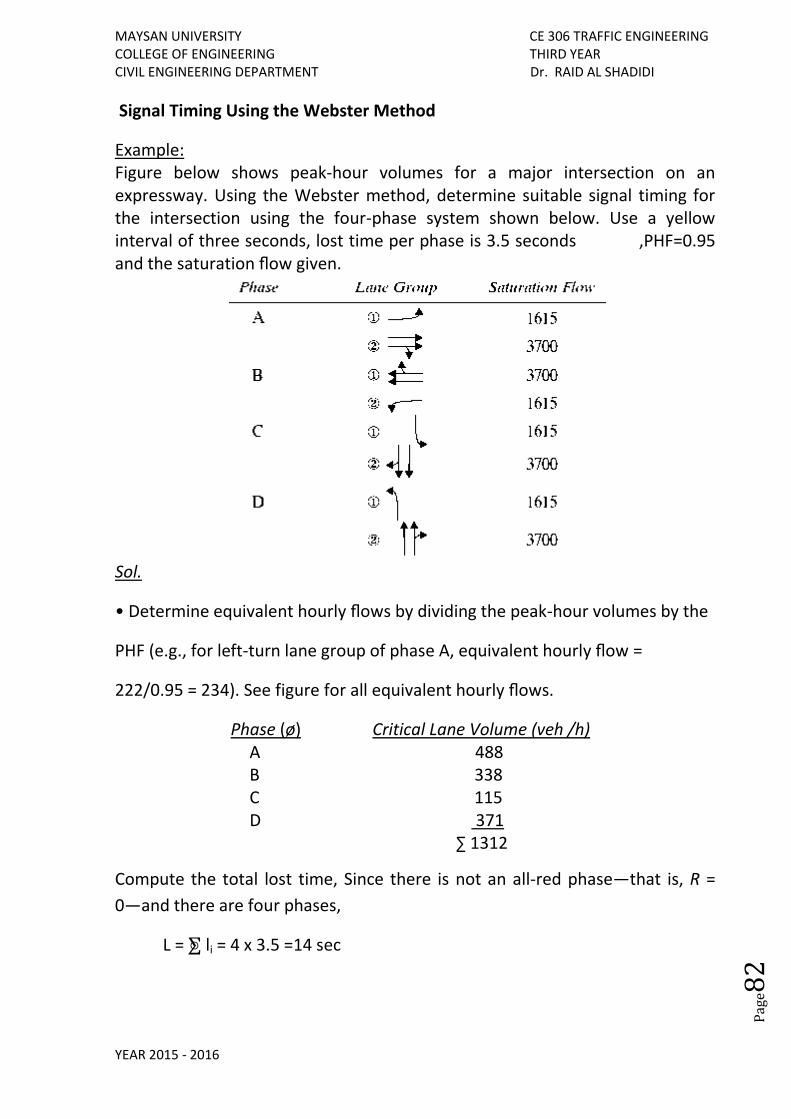
MAYSAN UNIVERSITY CE 306 TRAFFIC ENGINEERING COLLEGE OF ENGINEERING THIRD YEAR CIVIL ENGINEERING DEPARTMENT Dr. RAID AL SHADIDI
YEAR 2015 - 2016
Pag
e82
Signal Timing Using the Webster Method
Example: Figure below shows peak-hour volumes for a major intersection on an expressway. Using the Webster method, determine suitable signal timing for the intersection using the four-phase system shown below. Use a yellow interval of three seconds, lost time per phase is 3.5 seconds ,PHF=0.95 and the saturation flow given.
Sol.
• Determine equivalent hourly flows by dividing the peak-hour volumes by the
PHF (e.g., for left-turn lane group of phase A, equivalent hourly flow =
222/0.95 = 234). See figure for all equivalent hourly flows.
Phase (ø) Critical Lane Volume (veh /h) A 488 B 338 C 115 D 371 ∑ 1312
Compute the total lost time, Since there is not an all-red phase—that is, R =
0—and there are four phases,
L = ⨊ li = 4 x 3.5 =14 sec
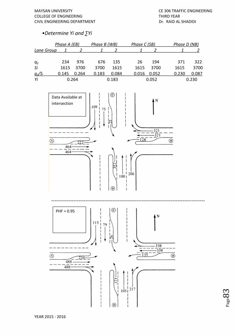
MAYSAN UNIVERSITY CE 306 TRAFFIC ENGINEERING COLLEGE OF ENGINEERING THIRD YEAR CIVIL ENGINEERING DEPARTMENT Dr. RAID AL SHADIDI
YEAR 2015 - 2016
Pag
e83
•Determine Yi and ∑Yi
Phase A (EB) Phase B (WB) Phase C (SB) Phase D (NB)
Lane Group 1 2 1 2 1 2 1 2 qij 234 976 676 135 26 194 371 322 Si 1615 3700 3700 1615 1615 3700 1615 3700 qij/Si 0.145 0.264 0.183 0.084 0.016 0.052 0.230 0.087 Yi 0.264 0.183 0.052 0.230
------------------------------------------------------------------------------------------
Data Available at
intersection
PHF = 0.95
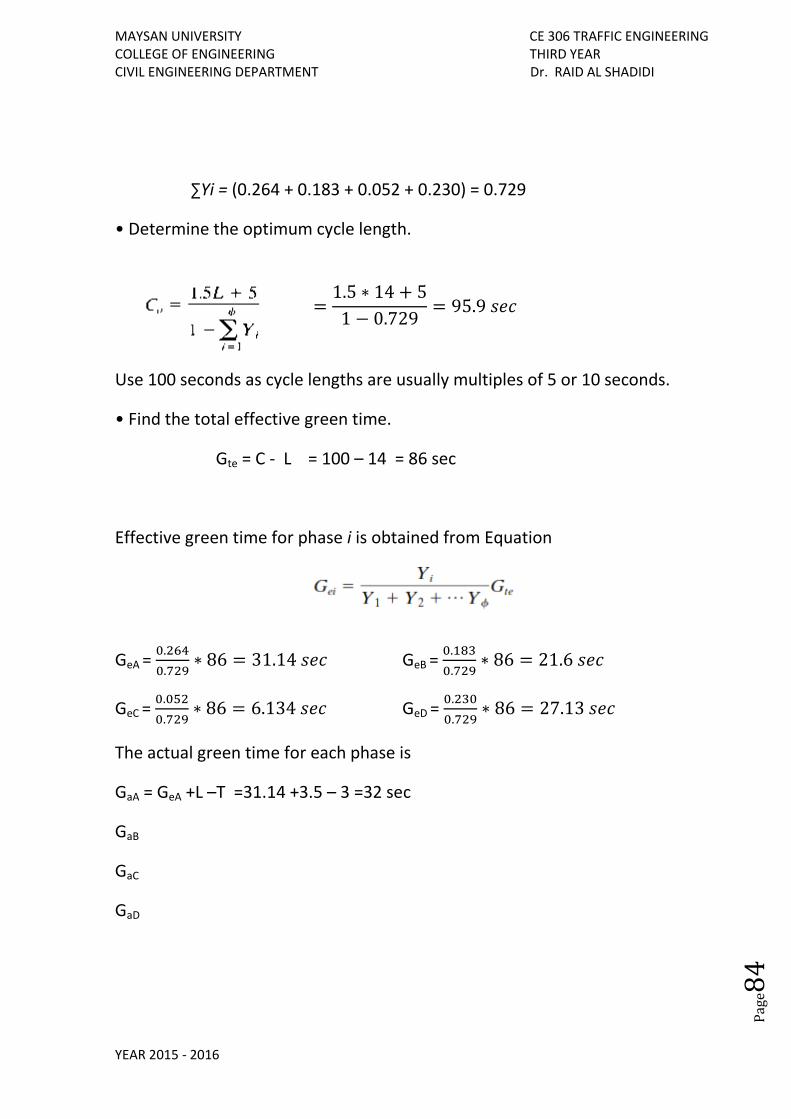
MAYSAN UNIVERSITY CE 306 TRAFFIC ENGINEERING COLLEGE OF ENGINEERING THIRD YEAR CIVIL ENGINEERING DEPARTMENT Dr. RAID AL SHADIDI
YEAR 2015 - 2016
Pag
e84
∑Yi = (0.264 + 0.183 + 0.052 + 0.230) = 0.729
• Determine the optimum cycle length.
=1.5 ∗ 14 + 5
1 − 0.729= 95.9 𝑠𝑒𝑐
Use 100 seconds as cycle lengths are usually multiples of 5 or 10 seconds.
• Find the total effective green time.
Gte = C - L = 100 – 14 = 86 sec
Effective green time for phase i is obtained from Equation
GeA = 0.264
0.729∗ 86 = 31.14 𝑠𝑒𝑐 GeB =
0.183
0.729∗ 86 = 21.6 𝑠𝑒𝑐
GeC = 0.052
0.729∗ 86 = 6.134 𝑠𝑒𝑐 GeD =
0.230
0.729∗ 86 = 27.13 𝑠𝑒𝑐
The actual green time for each phase is
GaA = GeA +L –T =31.14 +3.5 – 3 =32 sec
GaB
GaC
GaD
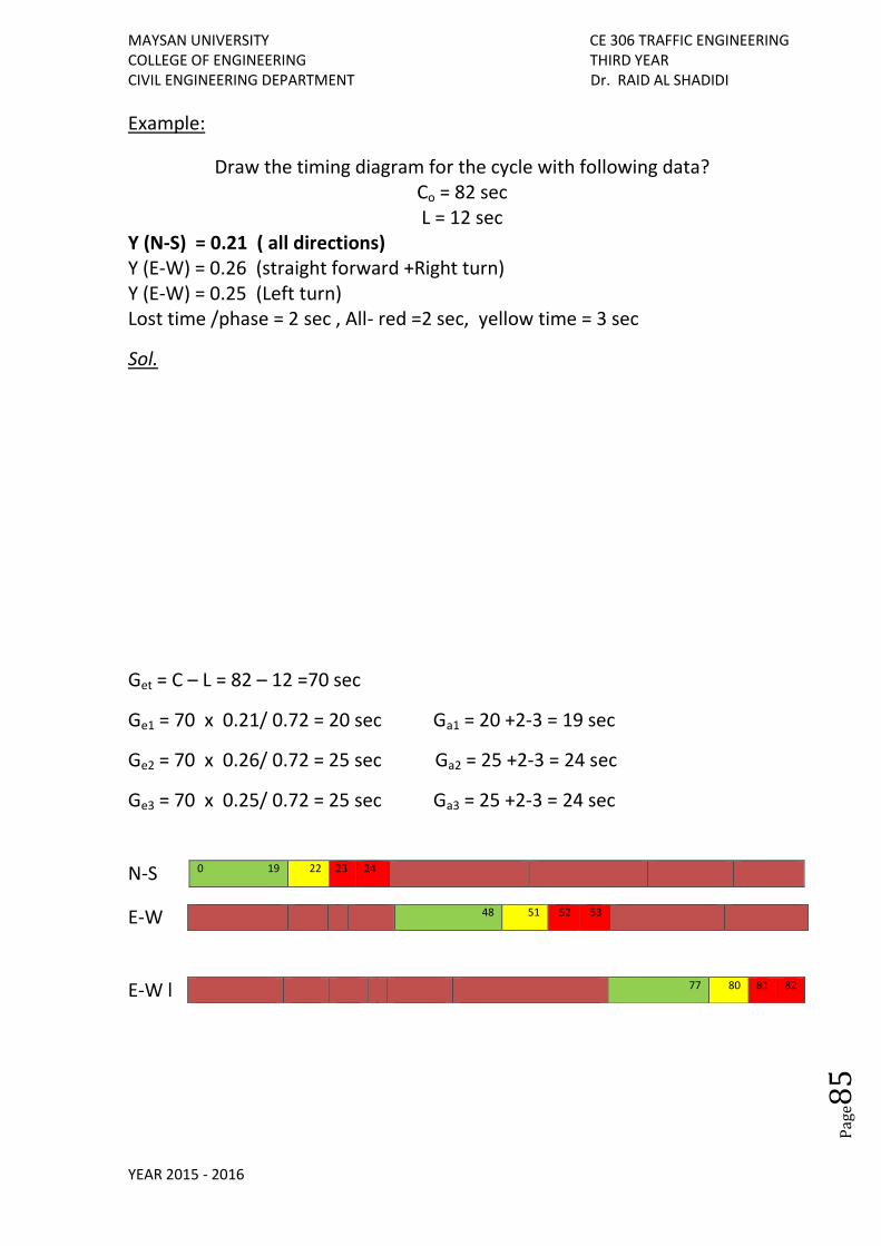
MAYSAN UNIVERSITY CE 306 TRAFFIC ENGINEERING COLLEGE OF ENGINEERING THIRD YEAR CIVIL ENGINEERING DEPARTMENT Dr. RAID AL SHADIDI
YEAR 2015 - 2016
Pag
e85
Example:
Draw the timing diagram for the cycle with following data? Co = 82 sec L = 12 sec
Y (N-S) = 0.21 ( all directions) Y (E-W) = 0.26 (straight forward +Right turn) Y (E-W) = 0.25 (Left turn) Lost time /phase = 2 sec , All- red =2 sec, yellow time = 3 sec
Sol.
Get = C – L = 82 – 12 =70 sec
Ge1 = 70 x 0.21/ 0.72 = 20 sec Ga1 = 20 +2-3 = 19 sec
Ge2 = 70 x 0.26/ 0.72 = 25 sec Ga2 = 25 +2-3 = 24 sec
Ge3 = 70 x 0.25/ 0.72 = 25 sec Ga3 = 25 +2-3 = 24 sec
N-S
E-W
E-W l
0 19 19 22 23 24
48 51 52 53
77 80 81 82
MAYSAN UNIVERSITY CE 306 TRAFFIC ENGINEERING COLLEGE OF ENGINEERING THIRD YEAR CIVIL ENGINEERING DEPARTMENT Dr. RAID AL SHADIDI
YEAR 2015 - 2016
Pag
e86
Parking
The provision of parking facilities is an essential element of the highway mode of transportation. The need for parking spaces is usually very great in areas where land uses include business, residential, or commercial activities. The growing use of the automobile as a personal feeder service to transit systems (“park-and-ride”) has also increased the demand for parking spaces at transit stations.
Types of Parking Facilities
1. On-Street Parking Facilities These are also known as curb facilities. Parking bays are provided alongside the curb on one or both sides of the street.
Marking Curb Stall
Parking stalls outlined or indicated on the pavement or curb are valuable in
promoting orderly parking. It is necessary to mark angle-parking stalls. The
American Automobile Association made a study of the time required to park in
uniformly marked 20 foot stalls, as compared with unmarked stretches of curb.
The findings were 21.7 second in average for marked stall over 38.4 second for
unmarked one.
2. Off-Street Parking Facilities These facilities may be privately or publicly owned; they include surface lots, multistory and underground garages.
Definitions of Parking Terms
1. A space-hour is a unit of parking that defines the use of a single parking space for a period of 1 hour.
2. Parking volume is the total number of vehicles that park in a study area during a specific length of time, usually a day.
3. Parking accumulation is the number of parked vehicles in a study area at any specified time. These data can be plotted as a curve of parking accumulation against time, which shows the variation of the parking accumulation during the day.
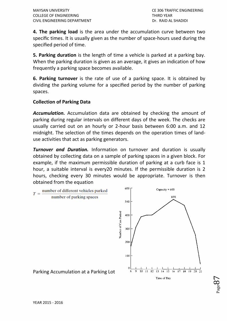
MAYSAN UNIVERSITY CE 306 TRAFFIC ENGINEERING COLLEGE OF ENGINEERING THIRD YEAR CIVIL ENGINEERING DEPARTMENT Dr. RAID AL SHADIDI
YEAR 2015 - 2016
Pag
e87
4. The parking load is the area under the accumulation curve between two specific times. It is usually given as the number of space-hours used during the specified period of time.
5. Parking duration is the length of time a vehicle is parked at a parking bay. When the parking duration is given as an average, it gives an indication of how frequently a parking space becomes available.
6. Parking turnover is the rate of use of a parking space. It is obtained by dividing the parking volume for a specified period by the number of parking spaces.
Collection of Parking Data
Accumulation. Accumulation data are obtained by checking the amount of parking during regular intervals on different days of the week. The checks are usually carried out on an hourly or 2-hour basis between 6:00 a.m. and 12 midnight. The selection of the times depends on the operation times of land-use activities that act as parking generators.
Turnover and Duration. Information on turnover and duration is usually obtained by collecting data on a sample of parking spaces in a given block. For example, if the maximum permissible duration of parking at a curb face is 1 hour, a suitable interval is every20 minutes. If the permissible duration is 2 hours, checking every 30 minutes would be appropriate. Turnover is then obtained from the equation
Parking Accumulation at a Parking Lot
MAYSAN UNIVERSITY CE 306 TRAFFIC ENGINEERING COLLEGE OF ENGINEERING THIRD YEAR CIVIL ENGINEERING DEPARTMENT Dr. RAID AL SHADIDI
YEAR 2015 - 2016
Pag
e88
Methodology of Parking Studies A comprehensive parking study usually involves (1) Inventory of existing parking facilities, (2) Collection of data on parking accumulation, parking turnover and parking
duration, (3) Identification of parking generators, and (4) Collection of information on parking demand. The space-hours of demand for parking are obtained from the expression
𝐷 = ∑(𝑛𝑖𝑡𝑖)
𝑁
𝑖=1
where D = space vehicle-hours demand for a specific period of time N = number of classes of parking duration ranges ti= mid parking duration of the ith class ni= number of vehicles parked for the ith duration range
The space-hours of supply are obtained from the expression
𝑆 = 𝑓 ∑(𝑡𝑖)
𝑁
𝑖=1
where S = practical number of space-hours of supply for a specific period of time N = number of parking spaces available ti = total length of time in hours when the ith space can be legally parked on during the specific period f = efficiency factor. Average values of f are 90 percent for curb parking, 80 percent for garages, and 85 percent for surface lots.
MAYSAN UNIVERSITY CE 306 TRAFFIC ENGINEERING COLLEGE OF ENGINEERING THIRD YEAR CIVIL ENGINEERING DEPARTMENT Dr. RAID AL SHADIDI
YEAR 2015 - 2016
Pag
e89
Space Requirements for a Parking Garage Example: The owner of a parking garage located in a CBD has observed that 20% of those wishing to park are turned back every day during the open hours of 8 a.m. to 6 p.m. because of lack of parking spaces. An analysis of data collected at the garage indicates that 60% of those who park are commuters, with an average parking duration of 9 hr, and the remaining are shoppers, whose average parking duration is 2 hr. If 20% of those who cannot park are commuters and the rest are shoppers, and a total of 200 vehicles currently park daily in the garage, determine the number of additional spaces required to meet the excess demand. Assume parking efficiency is 0.90. Sol. • Calculate the space-hours of demand using
𝐷 = ∑(𝑛𝑖𝑡𝑖)
𝑁
𝑖=1
Commuters now being served = 0.6 x 200 x 9 = 1080 space-hr Shoppers now being served = 0.4 x 200 x 2 = 160 space-hr Total number of vehicles turned away = 200 x0.2 /0.8 = 50 Commuters not being served = 0.2 x 50 x 9 = 90 space-hr Shoppers not being served = 0.8 x 50 x 2 = 80 space-hr Total space-hours of demand = (1080 + 160 + 90 + 80) = 1410 Total space-hours served = 1080 + 160 =1240 Number of space-hours required = 1410 - 1240 = 170 • Determine the number of parking spaces required
𝑆 = 𝑓 ∑ (𝑡𝑖)𝑁𝑖=1
= 170 space hr
• Use the length of time each space can be legally parked on (8 a.m. through 6 p.m. = 10 hr) to determine the number of additional spaces. 0.9 x 10 x N = 170 N = 18.89 At least 19 additional spaces will be required, since a fraction of a space cannot be used.
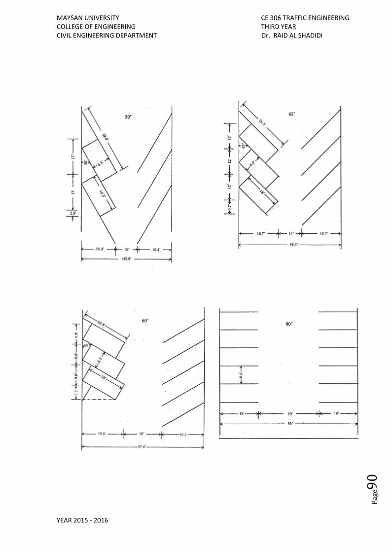
MAYSAN UNIVERSITY CE 306 TRAFFIC ENGINEERING COLLEGE OF ENGINEERING THIRD YEAR CIVIL ENGINEERING DEPARTMENT Dr. RAID AL SHADIDI
YEAR 2015 - 2016
Pag
e90
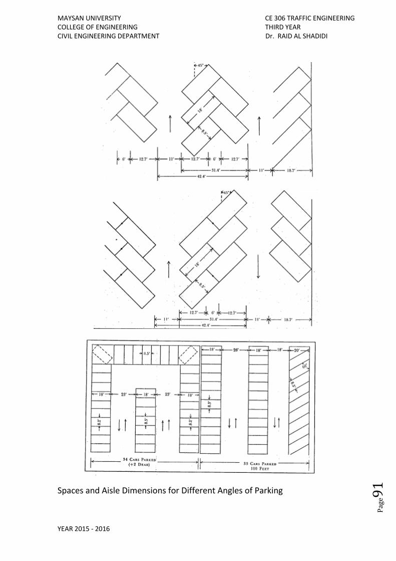
MAYSAN UNIVERSITY CE 306 TRAFFIC ENGINEERING COLLEGE OF ENGINEERING THIRD YEAR CIVIL ENGINEERING DEPARTMENT Dr. RAID AL SHADIDI
YEAR 2015 - 2016
Pag
e91
Spaces and Aisle Dimensions for Different Angles of Parking
MAYSAN UNIVERSITY CE 306 TRAFFIC ENGINEERING COLLEGE OF ENGINEERING THIRD YEAR CIVIL ENGINEERING DEPARTMENT Dr. RAID AL SHADIDI
YEAR 2015 - 2016
Pag
e92
Highway Safety
As the number of motor vehicles and vehicle-miles of travel increases throughout the world, the exposure of the population to traffic crashes also increases. Traffic and highway engineers are continually engaged in working to ensure that the street and highway system is designed and operated such that highway crash rates can be reduced. They also work with law-enforcement officials and educators in a team effort to ensure that traffic laws, such as those regarding speed limits and drinking, are enforced, and that motorists are educated about their responsibility to drive defensively and to understand and obey traffic regulations authority develop, establish, and implement systems for managing highway safety. There are five major safety programs that are addressed by authority in developing a safety management program. 1. Coordinating and integrating broad-based safety programs, such as motor carrier, corridor, and community-based safety activities, into a comprehensive management approach for highway safety.
2. Identifying and investigating hazardous highway safety problems and roadway locations and features, including railroad–highway grade crossings, and establishing countermeasures and priorities to correct identified or potential hazards.
3. Ensuring early consideration of safety in all highway construction programs and projects.
4. Identifying safety needs of special user groups (such as older drivers, pedestrians, bicyclists, motorcyclists, commercial motor carriers, and hazardous materials carriers) in the planning, design, construction, and operation of the highway system.
5. Routinely maintaining and upgrading safety hardware (including highway–rail crossing warning devices), highway elements, and operational features.
Factors Involved in Transportation Crashes
While the causes of crashes are usually complex and involve several factors, they can be considered in four separate categories:
MAYSAN UNIVERSITY CE 306 TRAFFIC ENGINEERING COLLEGE OF ENGINEERING THIRD YEAR CIVIL ENGINEERING DEPARTMENT Dr. RAID AL SHADIDI
YEAR 2015 - 2016
Pag
e93
Driver or Operator Action The major contributing cause of many crash situations is the performance of the driver of one or both (in multiple vehicle crashes) of the vehicles involved. Driver error can occur in many ways, such as inattention to the roadway and surrounding traffic, failure to yield the right of way, and/or traffic laws. These “failures” can occur as a result of unfamiliarity with roadway conditions, traveling at high speeds, drowsiness, drinking, and using a cell phone or other distractions within the vehicle.
The Vehicle Condition The mechanical condition of a vehicle can be the cause of transportation crashes. Faulty brakes in heavy trucks have caused crashes. Other reasons are failure of the electrical system, worn tires, and the location of the vehicle’s center of gravity.
The Roadway Condition The condition and quality of the roadway, which includes the pavement, shoulders, intersections, and the traffic control system, can be a factor in a crash. Highways must be designed to provide adequate sight distance at the design speed or motorists will be unable to take remedial action to avoid a crash. Traffic signals must provide adequate decision sight distance when the signal goes from green to red. Railroad grade crossings must be designed to operate safely and thus minimize crashes between highway traffic and rail cars. Highway curves must be carefully designed to accommodate Vehicles traveling at or below the design speed of the road. The Environment The physical and climatic environment surrounding a transportation vehicle can also be a factor in the occurrence of transportation crashes with the most common being weather. All transportation systems function at their best when the weather is sunny and mild and the skies are clear. Weather on roads can contribute to highway crashes; for example, wet pavement reduces stopping friction and can cause vehicles to hydroplane. Many severe crashes have been caused by fog because vehicles traveling at high speeds are unable to see other vehicles ahead that may have stopped or slowed down, creating a multivehicle pile-up. Geography is another environmental cause of transportation crashes. Mountain ranges have been the site of air crashes. Flooded river plains, swollen rivers, and mud slides on the pavement have caused railroad and highway crashes.
MAYSAN UNIVERSITY CE 306 TRAFFIC ENGINEERING COLLEGE OF ENGINEERING THIRD YEAR CIVIL ENGINEERING DEPARTMENT Dr. RAID AL SHADIDI
YEAR 2015 - 2016
Pag
e94
Highway Safety Improvement Program (HSIP) The planning component of the HSIP consists of four processes; these are
(1) Collecting and maintaining data,
(2) Identifying hazardous locations and elements,
(3) Conducting engineering studies, and
(4) Establishing project priorities.
Determining Possible Causes of Crashes
Having identified the hazardous locations and the crash pattern, the next stage
in the data analysis is to determine possible causes. The types of crashes
identified are matched with a list of possible causes from which several
probable causes are identified. The environmental conditions existing at the
time may also help in identifying possible causes.
Establishing Project Priorities
Economic Analysis
The purpose of this task is to determine the economic feasibility of each set of
countermeasures and to determine the best alternative among feasible
mutually exclusive countermeasures.
Conducting Engineering Studies After a particular location has been identified as hazardous, a detailed engineering study is performed to identify the safety problem. Once the safety problem is identified, suitable safety-related countermeasures can be developed.
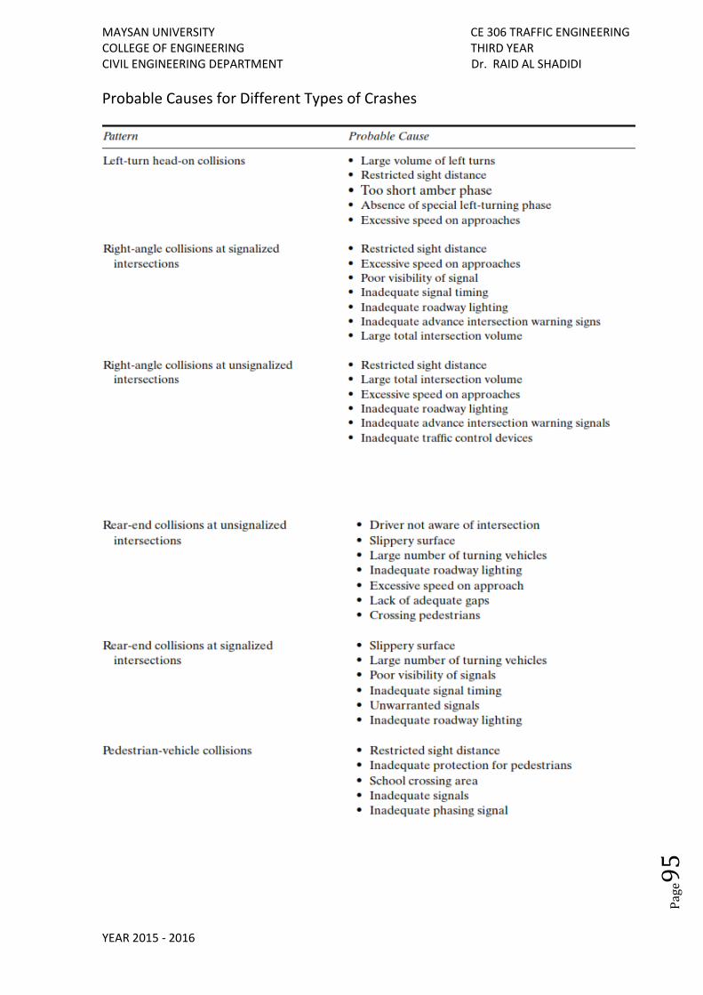
MAYSAN UNIVERSITY CE 306 TRAFFIC ENGINEERING COLLEGE OF ENGINEERING THIRD YEAR CIVIL ENGINEERING DEPARTMENT Dr. RAID AL SHADIDI
YEAR 2015 - 2016
Pag
e95
Probable Causes for Different Types of Crashes
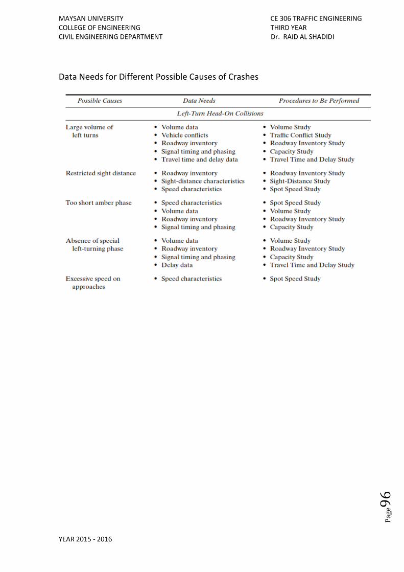
MAYSAN UNIVERSITY CE 306 TRAFFIC ENGINEERING COLLEGE OF ENGINEERING THIRD YEAR CIVIL ENGINEERING DEPARTMENT Dr. RAID AL SHADIDI
YEAR 2015 - 2016
Pag
e96
Data Needs for Different Possible Causes of Crashes
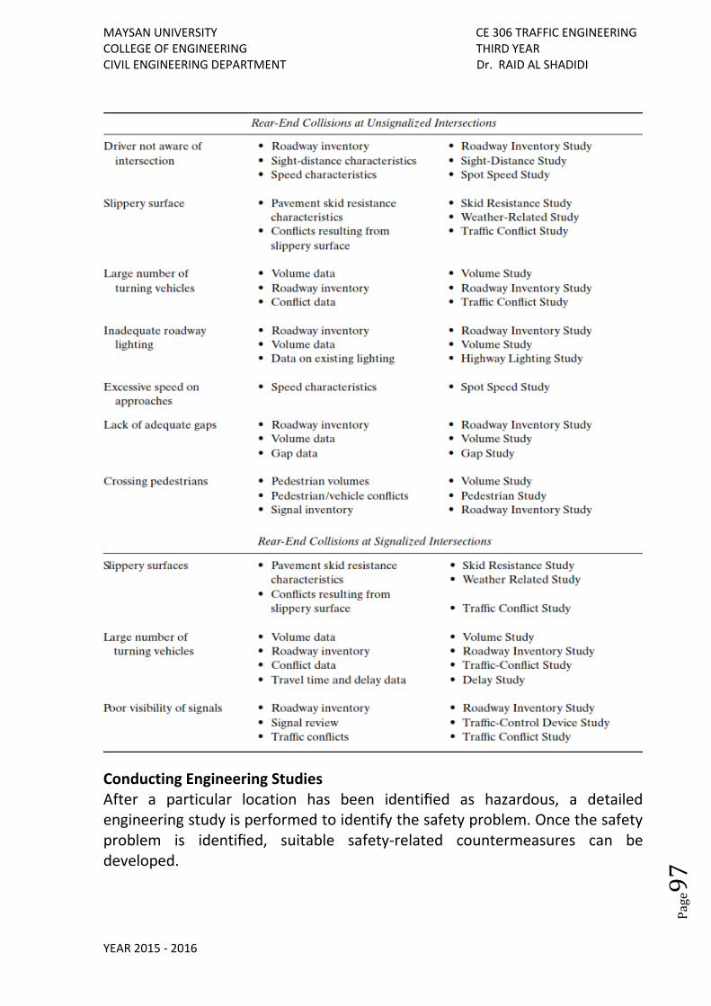
MAYSAN UNIVERSITY CE 306 TRAFFIC ENGINEERING COLLEGE OF ENGINEERING THIRD YEAR CIVIL ENGINEERING DEPARTMENT Dr. RAID AL SHADIDI
YEAR 2015 - 2016
Pag
e97
Conducting Engineering Studies After a particular location has been identified as hazardous, a detailed engineering study is performed to identify the safety problem. Once the safety problem is identified, suitable safety-related countermeasures can be developed.
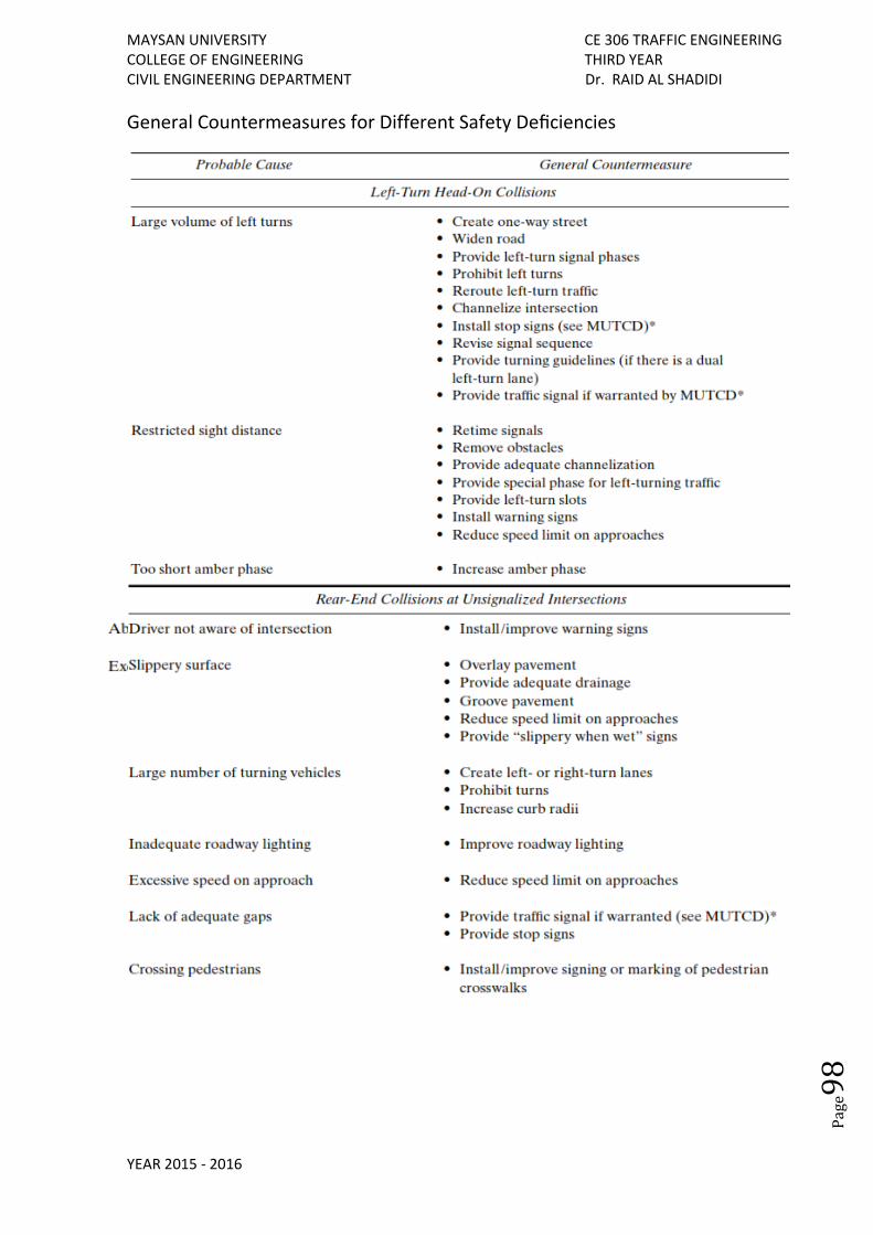
MAYSAN UNIVERSITY CE 306 TRAFFIC ENGINEERING COLLEGE OF ENGINEERING THIRD YEAR CIVIL ENGINEERING DEPARTMENT Dr. RAID AL SHADIDI
YEAR 2015 - 2016
Pag
e98
General Countermeasures for Different Safety Deficiencies
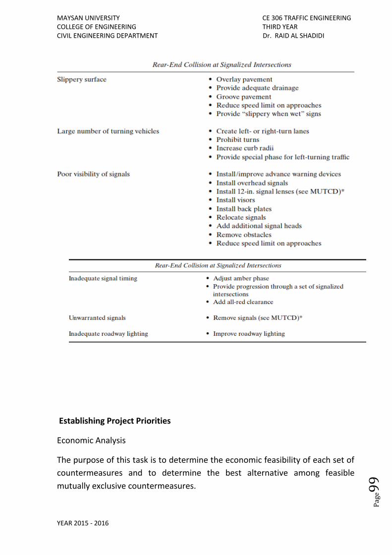
MAYSAN UNIVERSITY CE 306 TRAFFIC ENGINEERING COLLEGE OF ENGINEERING THIRD YEAR CIVIL ENGINEERING DEPARTMENT Dr. RAID AL SHADIDI
YEAR 2015 - 2016
Pag
e99
Establishing Project Priorities
Economic Analysis
The purpose of this task is to determine the economic feasibility of each set of
countermeasures and to determine the best alternative among feasible
mutually exclusive countermeasures.
MAYSAN UNIVERSITY CE 306 TRAFFIC ENGINEERING COLLEGE OF ENGINEERING THIRD YEAR CIVIL ENGINEERING DEPARTMENT Dr. RAID AL SHADIDI
YEAR 2015 - 2016
Pag
e10
0