1

CS347 Lecture 13

May 23, 2001

2

• Basic SQL• Relational algebra• Following aspects of centralized DB

– Query processing: query plans, cost estimation, optimization

– Concurrency control techniques– Recovery methods

3

• Primarily lecture notes• No required textbook• Some lecture material drawn from

M. Tamer Ozsu and Patrick Valduriez, "Principles of Distributed Database Systems," Second Edition, Prentice Hall 1999.

4

Software:ApplicationSQL Front EndQuery ProcessorTransaction Proc.File Access

P

M ...

• Simplifications:• single front end• one place to keep locks• if processor fails, system fails, …..

5

• Multiple processors, memories, and disks– Opportunity for parallelism (+)– Opportunity for enhanced reliability (+)– Synchronization issues (-)

• Heterogeneity and autonomy of “components”– Autonomy example: may not get statistics for query

optimization from a site

6

Select newinvestments

Application

RDBMS FilesStocktickertape

Portfolio History ofdividends,ratios,...

7

Data management with multiple processors and possible autonomy, heterogeneity. Impacts:

• Data organization• Query processing• Access structures• Concurrency control• Recovery

8

• Introductory topics– Database architectures– Distributed versus Parallel DB systems

• Distributed database design– Fragmentation– Allocation

9

Shared memory

P P P...

M

...

P

M

P

M...

P

M

Shared disk

10

P

M

...P

M

P

M

Shared nothing

Number of other “hybrid” architectures are possible.

11

• Reliability• Scalability• Geographic distribution of data• Performance• Cost

12

• Typically, parallel DBs:– Fast interconnect– Homogeneous software– Goals: High performance and Transparency

• Typically, distributed DBs:– Geographically distributed– Disconnected operation possible– Goal: Data sharing (heterogeneity, autonomy)

13

• Parallel DB: – Distribute/partition/sort…. data to make certain DB

operations (e.g., Join) fast

• Distributed DB:– Given data distribution, find query processing

strategy to minimize cost (e.g. communication cost)

14

Top-down approach:• have a database• how to split and allocate to individual sites

Multi-databases (or bottom-up):• combine existing databases• how to deal with heterogeneity & autonomy

15

• Fragmentation• Allocation

Note: issues not independent, but studiedseparately for simplicity.

16

Employee relation E (#,name,loc,sal,…)40% of queries: 40% of queries:

Qa: select * Qb: select *from E from Ewhere loc=Sa where loc=Sband… and ...

Motivation: Two sites: Sa, SbQa → ← QbSa Sb

17

# Name Loc Sal578

Sa 10Sally Sb 25Tom Sa 15

Joe

58

Sa 10Tom Sa 15Joe 7 Sb 25Sally

..

..

....

F = {F1,F2}

At Sa At Sb

E

F1 = σloc=Sa(E) F2 = σloc=Sb(E)

⇒ primary horizontal fragmentation

18

• Horizontal Primarydepends on local attributes

R Deriveddepends on foreign relation

• Vertical

R

19

• Round robin• Hash partitioning• Range partitioning

20

R F0 F1 F2

t1 t1t2 t2t3 t3t4 t4... t5

• Evenly distributes data• Good for scanning full relation• Not good for point or range queries

21

R F0 F1 F2

t1→h(k1)=2 t1t2→h(k2)=0 t2t3→h(k3)=0 t3t4→h(k4)=1 t4...

• Good for point queries on key; also for joins• Not good for range queries; point queries not on key• Good hash function even distribution

22

R F0 F1 F2

t1: A=5 t1t2: A=8 t2t3: A=2 t3t4: A=3 t4...

• Good for some range queries on A• Need to select good vector: else create imbalance

→ data skew→ execution skew

4 7

partitioningvector

V0 V1

23

Example 2: F = {F3,F4}F1 = σsal<10(E) F2 = σsal>5(E)

Example 1: F = {F1,F2}

F1 = σsal<10(E) F2 = σsal>20(E)

➽➽➽➽ Problem: Some tuples lost!

➽➽➽➽ Tuples with 5 < sal < 10 are duplicated

24

Prefer to deal with replication explicitly

Example: F = { F5, F6, F7 }

F5 = σsal<=5(E)F6 = σ5 < sal<10(E) F7 = σsal>=10(E)

�Then replicate F6 if desired as part of allocation

25

R ⇒ F = {F1,F2,….}(1) Completeness

∀∀∀∀t ∈∈∈∈ R, ∃∃∃∃ Fi ∈∈∈∈ F such that t ∈∈∈∈ Fi

(2) DisjointnessFi ∩ Fj = Ø, ∀∀∀∀ i,j such that i ≠ j

(3) Reconstruction∃∃∃∃ ∇∇∇∇ such that R = ∇∇∇∇ Fi

i

26

• Given simple predicates Pr = {p1, p2,.. pm} and relation R.

• Generate “minterm” predicates

M = {m | m = ∧∧∧∧ pk*, 1 ≤ k ≤ m}, wherepk* is either pk or ¬ pk

• Eliminate useless minterms and simplify M to get M’.

• Generate fragments σm(R) for each m ∈ M’.

27

• Example: say queries use predicates A < 10, A > 5, Loc = SA, Loc = SB

• Eliminate and simplify mintermsA < 10 ∧∧∧∧ A > 5 ∧∧∧∧ Loc = SA ∧∧∧∧ Loc = SBA < 10 ∧∧∧∧ A > 5 ∧∧∧∧ Loc = SA ∧∧∧∧ ¬(Loc = SB)

• Final set of fragments(5 < A < 10) ∧∧∧∧ (Loc = SA)(5 < A < 10) ∧∧∧∧ (Loc = SB)(A ≤ 5) ∧∧∧∧ (Loc = SA)(A ≤ 5) ∧∧∧∧ (Loc = SB)(A ≥ 10) ∧∧∧∧ (Loc = SA)(A ≥ 10) ∧∧∧∧ (Loc = SB)

Work out details for all minterms.

5 < A < 10

28

• Elimination of useless fragments/predicates depends on application semantics:– e.g.: if Loc ≠ SA and ≠ SB is possible, must retain

fragments such as (5 <A < 10) ∧∧∧∧ (Loc≠SA) ∧∧∧∧(Loc≠SB)

• Minterm-based fragmentation generates complete, disjoint, and reconstructible fragments. Justify this

statement.

29

• E (#,name,loc,sal,…) with common queriesQa: select * from E where loc = SA and…Qb: select * from E where loc = SB and…

• Three choices for Pr and hence F[Pr]:– Pr = {} F1 = F[Pr] = {E}– Pr = {Loc = SA, Loc = SB}

F2 = F[Pr] = {σloc=SA (E), σloc=SB (E)} – Pr = {Loc = SA, Loc = SB, Sal < 10}

F3 = F[Pr] = {σloc=SA ∧∧∧∧ sal< 10(E), σ loc=SB ∧∧∧∧ sal< 10(E),σloc=SA ∧∧∧∧ sal ≥ 10(E), σloc=SA ∧∧∧∧ sal ≥ 10 (E)}

30

Loc=SA ∧∧∧∧sal < 10

Loc=SA ∧∧∧∧

sal ≥ 10

Loc=SB ∧∧∧∧sal < 10

Loc=SB ∧∧∧∧

sal ≥ 10

F1

F3F2

Qa: Select … loc = SA ...

Qb: Select … loc = SB ...

Prefer F2 to F1 and F3

31

• CompletenessSet of predicates Pr is complete if for every Fi ∈ F[Pr], every t ∈ Fi has equal probabilityof access by every major application.

• MinimalitySet of predicates Pr is minimal if no Pr’ ⊂ Pr

is complete.

To get complete and minimal Pr use predicates that are “relevant” in frequent queries

Different from completeness of fragmentation

32

• Example: Two relations Employee and JobsE(#, NAME, SAL, LOC)J(#, DES,…)

• Fragment E into {E1, E2} by LOC

• Common query:“Given employee name, list projects (s)he works in”

33

E1

(at Sa) (at Sb)

E2# NM Loc Sal5 Joe Sa 108 Tom Sa 15…

# NM Loc Sal7 Sally Sb 2512 Fred Sb 15…

# Description5 work on 347 hw7 go to moon5 build table12 rest…

J

34

E1

(at Sa) (at Sb)

E2# NM Loc Sal5 Joe Sa 108 Tom Sa 15…

# NM Loc Sal7 Sally Sb 2512 Fred Sb 15…

J1 J2

J1 = J E1 J2 = J E2

# Des5 work on 347 hw5 build table…

# Des7 go to moon12 rest…

35

R, fragmented as F = {F1, F2, …, Fn}⇓⇓⇓⇓

S, derive D = {D1, D2, …, Dn} where Di =S Fi

Convention: R is called the owner relationS is called the member relation

36

• J1 U J2 ⊂ J (incomplete fragmentation)• For completeness, enforce referential integrity

constraintjoin attribute of member relation

⇓joint attribute of owner relation

# Des…33 build chair…

Example: Say J is

37

# NM Loc Sal5 Joe Sa 10…

# NM Loc Sal5 Fred Sb 20…

E1 E2

# Description5 day off…

# Description5 day off…

# Description5 day off…

J1

J

J2

Fragmentationis not

disjoint!

Common way to enforce disjointness: make join attribute key of owner relation.

38

E1

# NM Loc Sal5 Joe Sa 107 Sally Sb 258 Fred Sa 15…

# NM Loc5 Joe Sa7 Sally Sb8 Fred Sa…

# Sal5 107 258 15…

E

E2

Example:

R[T] ⇒ R1[T1], R2[T2],…, Rn[Tn] Ti ⊆ T

➽ Just like normalization of relations

39

R[T] ⇒ Ri[Ti], i = 1.. n

• Completeness: ∪Ti = T

• Reconstruction: Ri = R (lossless join)– One way to guarantee lossless join: repeat key in each

fragment, i.e., key ⊆⊆⊆⊆ Ti ∀∀∀∀ i

• Disjointness: Ti ∩ Tj = {key}– Check disjointness only on non-key attributes

40

E1(#,NM,LOC)E2(#,SAL)

Example:E(#,NM,LOC,SAL) E1(#,NM)

E2(#,LOC)E3(#,SAL)

Which is the right vertical fragmentation?…..

41

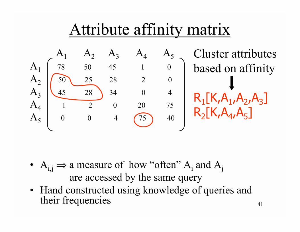
A1 A2 A3 A4 A5A1 78 50 45 1 0

A2 50 25 28 2 0

A3 45 28 34 0 4

A4 1 2 0 20 75

A5 0 0 4 75 40

• Ai,j ⇒ a measure of how “often” Ai and Ajare accessed by the same query

• Hand constructed using knowledge of queries and their frequencies

Cluster attributes based on affinity

R1[K,A1,A2,A3] R2[K,A4,A5]

42

Example: E ⇒ F1 = σloc=Sa(E); F2 = σloc=Sb(E)

Site aSite b

Fragment E

•Do we replicate fragments?

•Where do we place each copy of each fragment?

Site cF1

F1

F2

43

• Origin of queries• Communication cost and size of answers,

relations, etc.• Storage capacity, storage cost at sites, and size of

fragments• Processing power at the sites• Query processing strategy

– How are joins done? Where are answers collected?• Fragment replication

– Update cost, concurrency control overhead

44

• What is the best placement of fragments and/or best number of copies to:– minimize query response time– maximize throughput– minimize “some cost”– ...

• Subject to constraints– Available storage– Available bandwidth, processing power,…– Keep 90% of response time below X– ...

Very hard problem

45

• Query processing– Decomposition– Localization– Distributed query operators– Optimization (briefly)

46

• Ozsu and Valduriez. “Principles of Distributed Database Systems” – Chapter 5