1

Distributed Databases

CS347

Lecture 13

May 23, 2001

2

Expected Background

• Basic SQL

• Relational algebra

• Following aspects of centralized DB– Query processing: query plans, cost estimation,

optimization– Concurrency control techniques– Recovery methods

3

Reading Material

• Primarily lecture notes

• No required textbook

• Some lecture material drawn from

M. Tamer Ozsu and Patrick Valduriez, "Principles of Distributed Database Systems," Second Edition, Prentice Hall 1999.

4

Centralized DBMS

Software:

ApplicationSQL Front EndQuery ProcessorTransaction Proc.File Access

P

M ...

• Simplifications:• single front end

• one place to keep locks

• if processor fails, system fails, …..

5

Distributed DB

• Multiple processors, memories, and disks– Opportunity for parallelism (+)– Opportunity for enhanced reliability (+)– Synchronization issues (-)

• Heterogeneity and autonomy of “components”– Autonomy example: may not get statistics for query

optimization from a site

6

Heterogeneity

Select new

investments Application

RDBMS FilesStocktickertape

Portfolio History ofdividends,ratios,...

7

Data management with multiple processors and possible autonomy, heterogeneity. Impacts:

• Data organization• Query processing• Access structures• Concurrency control• Recovery

Big Picture

8

Today’s topics

• Introductory topics– Database architectures– Distributed versus Parallel DB systems

• Distributed database design– Fragmentation– Allocation

9

Common DB architectures

Shared memory

P P P...

M

...

P

M

P

M...

P

M

Shared disk

10

Common DB architectures

P

M

...P

M

P

M

Shared nothing

Number of other “hybrid” architectures are possible.

11

Selecting the “right” architecture

• Reliability

• Scalability

• Geographic distribution of data

• Performance

• Cost

12

Parallel vs. Distributed DB system• Typically, parallel DBs:

– Fast interconnect– Homogeneous software– Goals: High performance and Transparency

• Typically, distributed DBs:– Geographically distributed– Disconnected operation possible– Goal: Data sharing (heterogeneity, autonomy)

13

Typical query processing scenarios

• Parallel DB: – Distribute/partition/sort…. data to make certain DB

operations (e.g., Join) fast

• Distributed DB:– Given data distribution, find query processing

strategy to minimize cost (e.g. communication cost)

14

Distributed DB Design

Top-down approach:

• have a database

• how to split and allocate to individual sites

Multi-databases (or bottom-up):

• combine existing databases

• how to deal with heterogeneity & autonomy

15

Two issues in top-down design

• Fragmentation

• Allocation

Note: issues not independent, but studied

separately for simplicity.

16

Example

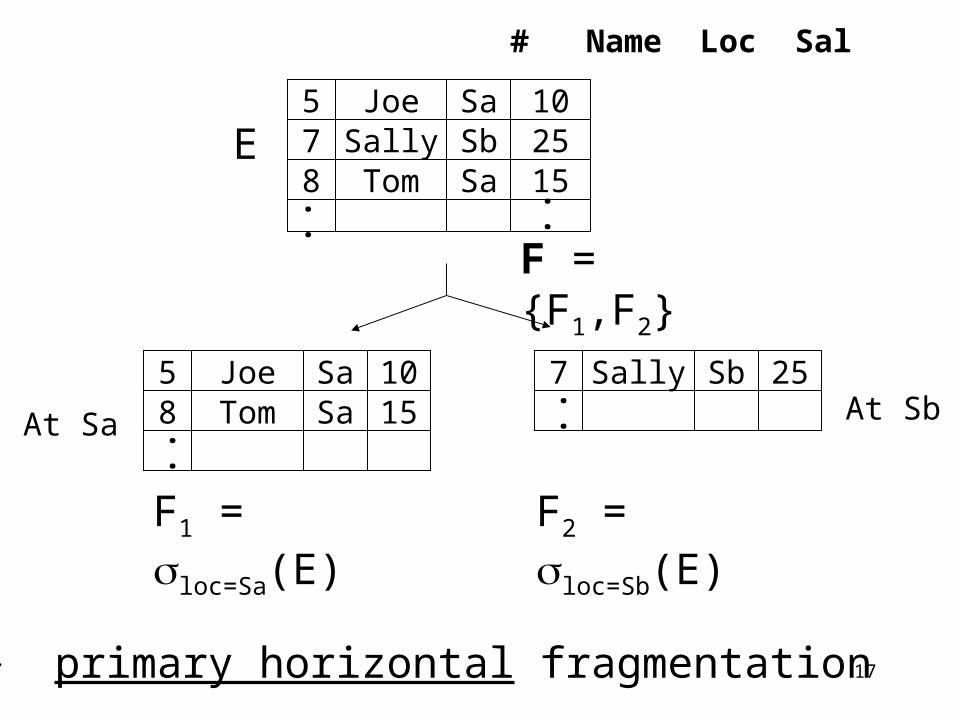
Employee relation E (#,name,loc,sal,…)

40% of queries: 40% of queries:

Qa: select * Qb: select *

from E from E

where loc=Sa where loc=Sb

and… and ...

Motivation: Two sites: Sa, Sb

Qa QbSa Sb

17

# Name Loc Sal

578

Sa 10Sally Sb 25Tom Sa 15

Joe

58

Sa 10Tom Sa 15Joe 7 Sb 25Sally

..

..

....

F = {F1,F2}

At Sa At Sb

E

F1 = loc=Sa(E) F2 = loc=Sb(E)

primary horizontal fragmentation

18

Fragmentation• Horizontal Primary

depends on local attributes

R Derived depends on foreign

relation

• Vertical

R

19

Horizontal partitioning techniques

• Round robin

• Hash partitioning

• Range partitioning

20

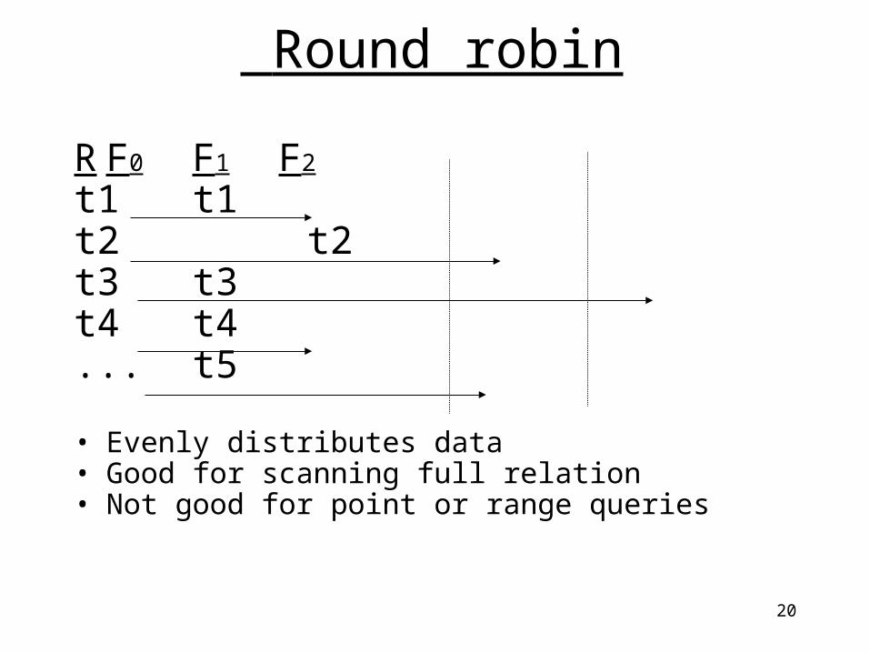
Round robin

R F0 F1 F2

t1 t1t2 t2t3 t3t4 t4... t5

• Evenly distributes data• Good for scanning full relation• Not good for point or range queries

21

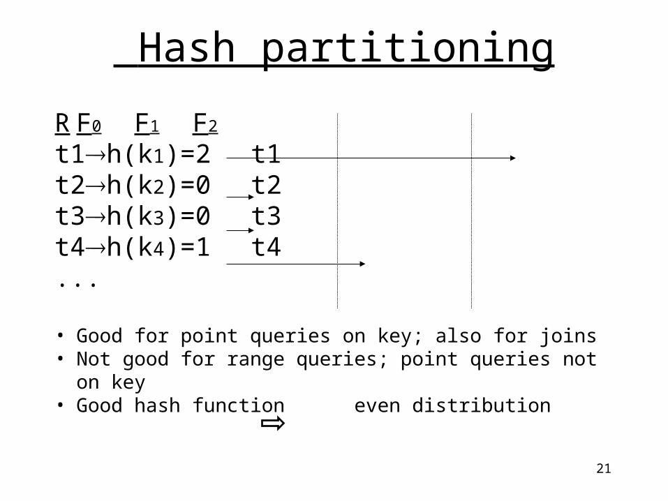
Hash partitioning

R F0 F1 F2

t1h(k1)=2 t1t2h(k2)=0 t2t3h(k3)=0 t3t4h(k4)=1 t4...

• Good for point queries on key; also for joins• Not good for range queries; point queries not on key• Good hash function even distribution

22

Range partitioning

R F0 F1 F2

t1: A=5 t1t2: A=8 t2t3: A=2 t3t4: A=3 t4...

• Good for some range queries on A• Need to select good vector: else create imbalance data skew execution skew

4 7

partitioningvector

V0 V1

23

Which are good fragmentations?

Example 2: F = {F3,F4}

F1 = sal<10(E) F2 = sal>5(E)

Example 1: F = {F1,F2}

F1 = sal<10(E) F2 = sal>20(E)

Problem: Some tuples lost!

Tuples with 5 < sal < 10 are duplicated

24

Prefer to deal with replication explicitly

Example: F = { F5, F6, F7 }

F5 = sal<=5(E) F6 = 5 < sal<10(E) F7 = sal>=10(E)

Then replicate F6 if desired as part of allocation

25

Horizontal Fragmentation Desiderata

R F = {F1,F2,….}

(1) Completeness

t R, Fi F such that t Fi

(2) Disjointness

Fi Fj = Ø, i,j such that i j

(3) Reconstruction

such that R = Fi

i

26

Generating horizontal fragments• Given simple predicates Pr = {p1, p2,.. pm} and

relation R.

• Generate “minterm” predicates

M = {m | m = pk*, 1 k m}, where

pk* is either pk or ¬ pk

• Eliminate useless minterms and simplify M to get M’.

• Generate fragments m(R) for each m M’.

27

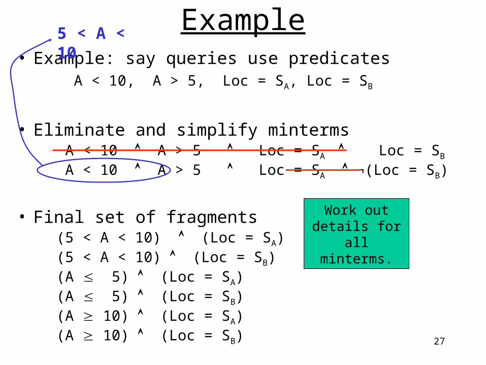
• Example: say queries use predicates A < 10, A > 5, Loc = SA, Loc = SB

• Eliminate and simplify minterms A < 10 A > 5 Loc = SA Loc = SB

A < 10 A > 5 Loc = SA ¬(Loc = SB)

• Final set of fragments (5 < A < 10) (Loc = SA) (5 < A < 10) (Loc = SB) (A 5) (Loc = SA) (A 5) (Loc = SB) (A 10) (Loc = SA) (A 10) (Loc = SB)

Example

Work out details for all minterms.

5 < A < 10

28

More on Horizontal Fragmentation• Elimination of useless fragments/predicates

depends on application semantics:– e.g.: if Loc SA and SB is possible, must retain

fragments such as (5 <A < 10) (LocSA) (LocSB)

• Minterm-based fragmentation generates complete, disjoint, and reconstructible fragments. Justify this

statement.

29

Choosing simple predicates• E (#,name,loc,sal,…) with common queries

Qa: select * from E where loc = SA and…

Qb: select * from E where loc = SB and…

• Three choices for Pr and hence F[Pr]:

– Pr = {} F1 = F[Pr] = {E}

– Pr = {Loc = SA, Loc = SB}

F2 = F[Pr] = {loc=SA (E), loc=SB (E)}

– Pr = {Loc = SA, Loc = SB, Sal < 10}

F3 = F[Pr] = {loc=SA sal< 10(E), loc=SB sal< 10(E),

loc=SA sal 10(E), loc=SA sal 10 (E)}

30

Loc=SA sal < 10

Loc=SA

sal 10

Loc=SB sal < 10

Loc=SB

sal 10

F1

F3F2

Qa: Select … loc = SA ...

Qb: Select … loc = SB ...

Prefer F2 to F1 and F3

31

Desiderata for simple predicates• Completeness

Set of predicates Pr is complete if for every

Fi F[Pr], every t Fi has equal probability

of access by every major application.

• Minimality

Set of predicates Pr is minimal if no Pr’ Pr

is complete.

To get complete and minimal Pr use predicates that are “relevant” in frequent queries

Different from completeness of fragmentation

32

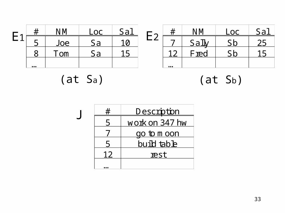
Derived horizontal fragmentation• Example: Two relations Employee and Jobs

E(#, NAME, SAL, LOC)

J(#, DES,…)

• Fragment E into {E1, E2} by LOC

• Common query:

“Given employee name, list projects (s)he works in”

33

E1

(at Sa) (at Sb)

E2# NM Loc Sal5 Joe Sa 108 Tom Sa 15…

# NM Loc Sal7 Sally Sb 2512 Fred Sb 15…

# Description5 work on 347 hw7 go to moon5 build table12 rest…

J

34

E1

(at Sa) (at Sb)

E2# NM Loc Sal5 Joe Sa 108 Tom Sa 15…

# NM Loc Sal7 Sally Sb 2512 Fred Sb 15…

J1 J2

J1 = J E1 J2 = J E2

# Des5 work on 347 hw5 build table…

# Des7 go to moon12 rest…

35

Derived horizontal fragmentationR, fragmented as F = {F1, F2, …, Fn}

S, derive D = {D1, D2, …, Dn} where Di =S Fi

Convention: R is called the owner relation

S is called the member relation

36

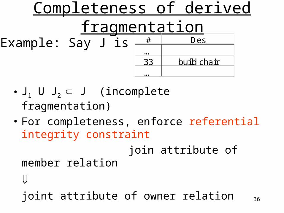
Completeness of derived fragmentation

• J1 U J2 J (incomplete fragmentation)

• For completeness, enforce referential integrity constraint

join attribute of member relation

joint attribute of owner relation

# Des…33 build chair…

Example: Say J is

37

# NM Loc Sal5 Joe Sa 10…

# NM Loc Sal5 Fred Sb 20…

E1 E2

# Description5 day off…

# Description5 day off…

# Description5 day off…

J1

J

J2

Fragmentationis not

disjoint!

Common way to enforce disjointness: make join attribute key of owner relation.

38

Vertical fragmentation

E1

# NM Loc Sal5 Joe Sa 107 Sally Sb 258 Fred Sa 15…

# NM Loc5 Joe Sa7 Sally Sb8 Fred Sa…

# Sal5 107 258 15…

E

E2

Example:

R[T] R1[T1], R2[T2],…, Rn[Tn] Ti T

Just like normalization of relations

39

PropertiesR[T] Ri[Ti], i = 1.. n

• Completeness: Ti = T

• Reconstruction: Ri = R (lossless join)

– One way to guarantee lossless join: repeat key in each fragment, i.e., key Ti i

• Disjointness: Ti Tj = {key}

– Check disjointness only on non-key attributes

40

E1(#,NM,LOC)

E2(#,SAL)

Example:

E(#,NM,LOC,SAL) E1(#,NM)

E2(#,LOC)

E3(#,SAL)

Which is the right vertical fragmentation?

…..

Grouping Attributes

41

A1 A2 A3 A4 A5

A1 78 50 45 1 0

A2 50 25 28 2 0

A3 45 28 34 0 4

A4 1 2 0 20 75

A5 0 0 4 75 40

• Ai,j a measure of how “often” Ai and Aj are accessed by the same query• Hand constructed using knowledge of queries and

their frequencies

Attribute affinity matrixCluster attributes based on affinity

R1[K,A1,A2,A3] R2[K,A4,A5]

42

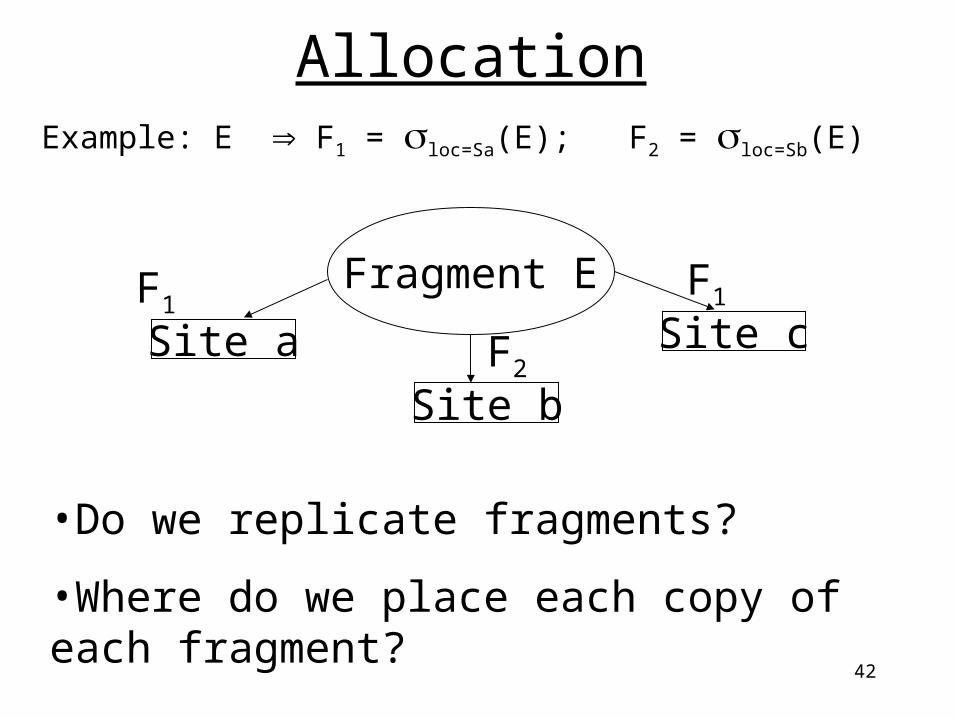
Allocation

Example: E F1 = loc=Sa(E); F2 = loc=Sb(E)

Site a

Site b

Fragment E

•Do we replicate fragments?

•Where do we place each copy of each fragment?

Site cF1

F1

F2

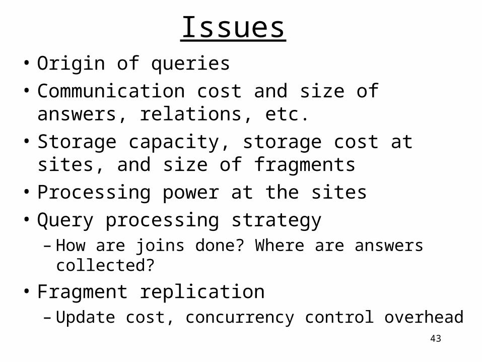
43

Issues• Origin of queries

• Communication cost and size of answers, relations, etc.

• Storage capacity, storage cost at sites, and size of fragments

• Processing power at the sites

• Query processing strategy– How are joins done? Where are answers collected?

• Fragment replication– Update cost, concurrency control overhead

44

Optimization problem• What is the best placement of fragments and/or

best number of copies to:– minimize query response time– maximize throughput– minimize “some cost”– ...

• Subject to constraints– Available storage– Available bandwidth, processing power,…– Keep 90% of response time below X– ...

Very hard problem

45

Looking Ahead• Query processing

– Decomposition– Localization– Distributed query operators– Optimization (briefly)

46

Resources

• Ozsu and Valduriez. “Principles of Distributed Database Systems” – Chapter 5