MaximumLikelihood Estimation of Migration ates and

Copyright 1999 by the Genetics Society of America

Maximum-Likelihood Estimation of Migration Rates and Effective PopulationNumbers in Two Populations Using a Coalescent Approach

Peter Beerli and Joseph FelsensteinDepartment of Genetics, University of Washington, Box 357360, Seattle, Washington 98195-7360

Manuscript received January 5, 1998Accepted for publication February 23, 1999

ABSTRACTA new method for the estimation of migration rates and effective population sizes is described. It

uses a maximum-likelihood framework based on coalescence theory. The parameters are estimated byMetropolis-Hastings importance sampling. In a two-population model this method estimates four parame-ters: the effective population size and the immigration rate for each population relative to the mutationrate. Summarizing over loci can be done by assuming either that the mutation rate is the same for allloci or that the mutation rates are gamma distributed among loci but the same for all sites of a locus.The estimates are as good as or better than those from an optimized FST -based measure. The program isavailable on the World Wide Web at http://evolution.genetics.washington.edu/lamarc.html/.

SEVERAL methods for the estimation of migration and migration events. This should be superior to pair-wise estimators such as those using FST or related statisticsrates between subpopulations have been proposed.

We can subdivide them into two very different ap- (cf. Felsenstein 1992b) and also more powerful thanthe cladistic approach of Slatkin and Maddisonproaches: (1) marking individuals and tracking their

individual movements and then extrapolating these in- (1989), which needs to know the true genealogy. Ourapproach estimates similar parameters as the programdividual movements to migration rates; or (2) surveying

genetic markers in the populations of interest and calcu- of Bahlo and Griffiths (http://www.maths.monash.edu.au/!mbahlo/mpg/gtree.html/),which is based on thelating a migration rate from allele frequencies or se-

quence differences. Of course, one should be aware work of Griffiths and Tavare (1994) and Nath andGriffiths (1996). It differs in the way we search thethat these two approaches do not estimate the same

quantity: approach 1 estimates the actual “instantane- genealogy space, and our methods support mutationmodels for different types of data: the infinite alleleous” migration rate of individuals, whereas approach 2

reflects an average over a time period whose length is model for electrophoretic markers, a one-stepmodel formicrosatellites, and a finite-sites model for nucleotidedetermined by the rate of mutation per generation of

the locus under study or by the time scale of genetic sequences. The sequence model is more useful thanthe infinite sites model, which forces the researcher todrift. The genetic approach tends to gives a lower esti-

mate than the individual migration rates approach be- discard data when there are multiple mutations at thesame sites.cause the method is looking at changes that become

established in the subpopulation gene pool.Current estimation methods for genetic data are

MODELmethods such as those related to FST (e.g., Slatkin 1991;Slatkin and Hudson 1991), the rare allele approach of We propose amethod to make amaximum-likelihoodSlatkin (1985), a maximum-likelihood method using estimate of population parameters for geographicallygene frequency distributions (Rannala and Hartigan subdivided populations. The general outline of such1996; Tufto et al. 1996), and approaches based on coa- estimates involves extending coalescence theory (King-lescent theory (Kingman 1982a,b), such as the cladis- man 1982a,b) to include migration events. Migrationtic approach of Slatkin and Maddison (1989), the models with coalescents were first developed by Taka-method outlined in Wakeley (1998), and maximum hata (1988) and Takahata and Slatkin (1990) forlikelihood using coalescent theory (Nath and Grif- two gene copies and discussed more generally for nfiths 1993, 1996). We describe here a new method us- gene copies in two populations by Hudson (1990), withing a maximum-likelihood- and coalescent theory-based generalization to multiple populations and differentapproach. models of migration by Notohara (1990). Nath and

Our method integrates over all possible genealogies Griffiths (1993, 1996) used this migration-coalescentprocess for maximum-likelihood estimation of one pa-rameter, the effective number of migrants ! " 4Nem,

Corresponding author:PeterBeerli, J255Health Sciences, Departmentwhere Ne is the effective population size and m is theofGenetics, University of Washington, Box 357360, Seattle,WA 98195-

7360. E-mail: [email protected] migration rate per generation.

Genetics 152: 763–773 ( June 1999)

764 P. Beerli and J. Felsenstein

results could not be extended to cases with geographicalstructure. They were unable to obtain the distributionof times to coalescence in the presence of migration.We have avoided this difficulty by having the genealogyG specify not only the coalescences but also the times

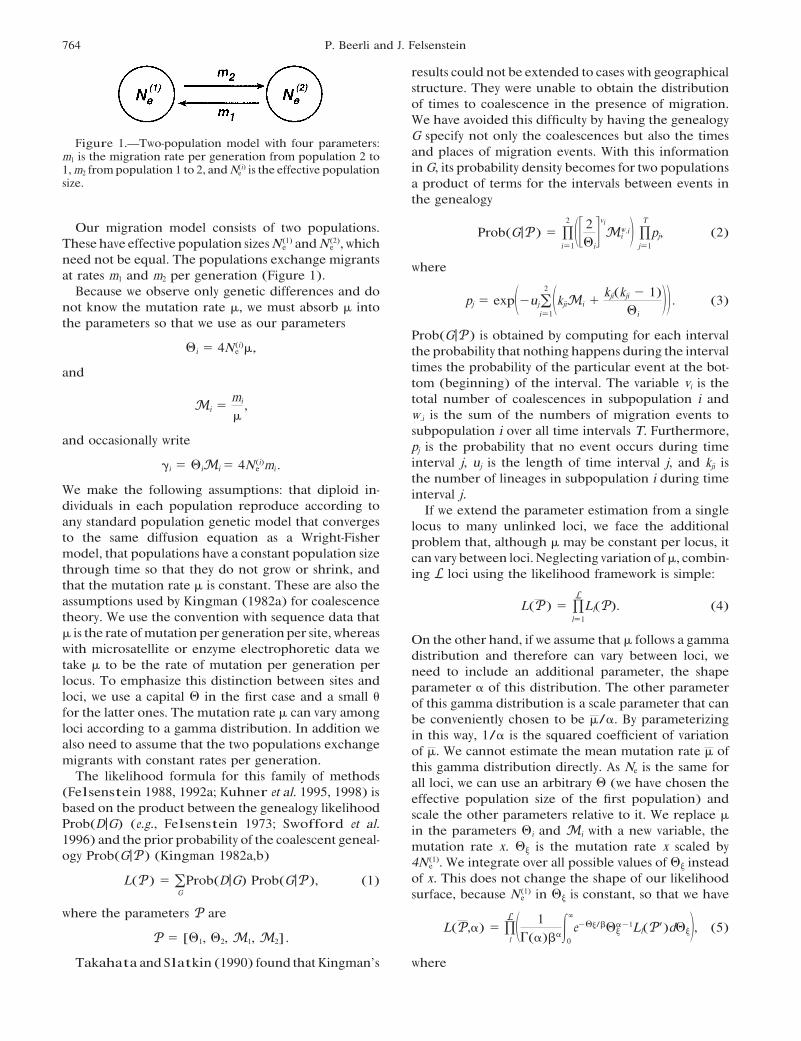
Figure 1.—Two-population model with four parameters:and places of migration events. With this informationm1 is the migration rate per generation from population 2 toin G, its probability density becomes for two populations1,m2 frompopulation 1 to 2, andN(i)

e is the effective populationsize. a product of terms for the intervals between events in

the genealogy

Our migration model consists of two populations. Prob(G|P) " !2

i"1"# 2

#i$viMw.i

i % !T

j"1

pj, (2)These have effective population sizesN (1)

e andN (2)e ,which

need not be equal. The populations exchange migrants whereat rates m1 and m2 per generation (Figure 1).

Because we observe only genetic differences and dopj " exp"$uj&

2

i"1"kjiMi %

kji(kji $ 1)#i

%% . (3)not know the mutation rate &, we must absorb & intothe parameters so that we use as our parameters

Prob(G|P) is obtained by computing for each interval#i " 4N (i)

e &, the probability that nothing happens during the intervaltimes the probability of the particular event at the bot-andtom (beginning) of the interval. The variable vi is thetotal number of coalescences in subpopulation i andMi "

mi

&,

w.i is the sum of the numbers of migration events tosubpopulation i over all time intervals T. Furthermore,

and occasionally write pj is the probability that no event occurs during timeinterval j, uj is the length of time interval j, and kji is!i " #iMi " 4N (i)

e mi .the number of lineages in subpopulation i during time

We make the following assumptions: that diploid in- interval j.dividuals in each population reproduce according to If we extend the parameter estimation from a singleany standard population genetic model that converges locus to many unlinked loci, we face the additionalto the same diffusion equation as a Wright-Fisher problem that, although & may be constant per locus, itmodel, that populations have a constant population size can vary between loci. Neglecting variation of&, combin-through time so that they do not grow or shrink, and ing L loci using the likelihood framework is simple:that the mutation rate & is constant. These are also theassumptions used by Kingman (1982a) for coalescence L(P) " !

L

l"1

Ll(P). (4)theory. We use the convention with sequence data that& is the rate ofmutation per generation per site,whereas On the other hand, if we assume that & follows a gammawith microsatellite or enzyme electrophoretic data we distribution and therefore can vary between loci, wetake & to be the rate of mutation per generation per need to include an additional parameter, the shapelocus. To emphasize this distinction between sites and parameter ' of this distribution. The other parameterloci, we use a capital # in the first case and a small ( of this gamma distribution is a scale parameter that canfor the latter ones. The mutation rate & can vary among be conveniently chosen to be &/'. By parameterizingloci according to a gamma distribution. In addition we in this way, 1/' is the squared coefficient of variationalso need to assume that the two populations exchange of &. We cannot estimate the mean mutation rate & ofmigrants with constant rates per generation. this gamma distribution directly. As Ne is the same for

The likelihood formula for this family of methods all loci, we can use an arbitrary # (we have chosen the(Felsenstein 1988, 1992a; Kuhner et al. 1995, 1998) is effective population size of the first population) andbased on the product between the genealogy likelihood scale the other parameters relative to it. We replace &Prob(D|G) (e.g., Felsenstein 1973; Swofford et al. in the parameters #i and Mi with a new variable, the1996) and the prior probability of the coalescent geneal- mutation rate x. #) is the mutation rate x scaled byogy Prob(G|P) (Kingman 1982a,b) 4N (1)

e . We integrate over all possible values of #) insteadof x. This does not change the shape of our likelihoodL(P) " &

GProb(D|G) Prob(G|P), (1)

surface, because N (1)e in #) is constant, so that we have

where the parameters P areL(P,') " !

L

l" 1*(')+''

∞

0

e$#)/+#'$1) Ll(P,)d#)%, (5)

P " [#1, #2, M1, M2] .

Takahata and Slatkin (1990) found thatKingman’s where

765Estimation of Population Parameters

In the program Coalesce (Kuhner et al. 1995) a re-+ "

#1

', gion of internal nodes in the genealogy is erased and

rebuilt according to the coalescent model. This schemeP, " ##), #2

#)

#1

, M())1 , M())

2 $, is not applicable to migration models. We adopt a newscheme that is much more general and that can be#) " 4N(1)

e x,used in any extension to the coalescent model. The first

and genealogy for each locus is constructed with a UPGMAmethod (as implemented byM.K.Kuhner and J. Yamatoin Felsenstein 1993), and theminimal necessarymigra-M())

i "!i

#i

#1

#)

.tion events are inserted using a Fitch parsimony algo-rithm (Fitch 1971). The times for coalescent events orThis integral over all mutation rate values is imple-migration events on this first genealogy are calculatedmented using a discrete gamma approximation withwith (3) using a uniform random number for pj and100 intervals (cf. Yang 1994).solving for uj, and parameter values, which are eitherNote that the gamma distribution described here isguessed by the researcher or calculated using an FST -the distribution of& across loci, not themore commonlybased method (see appendix).used gamma distribution of rates across sites within a

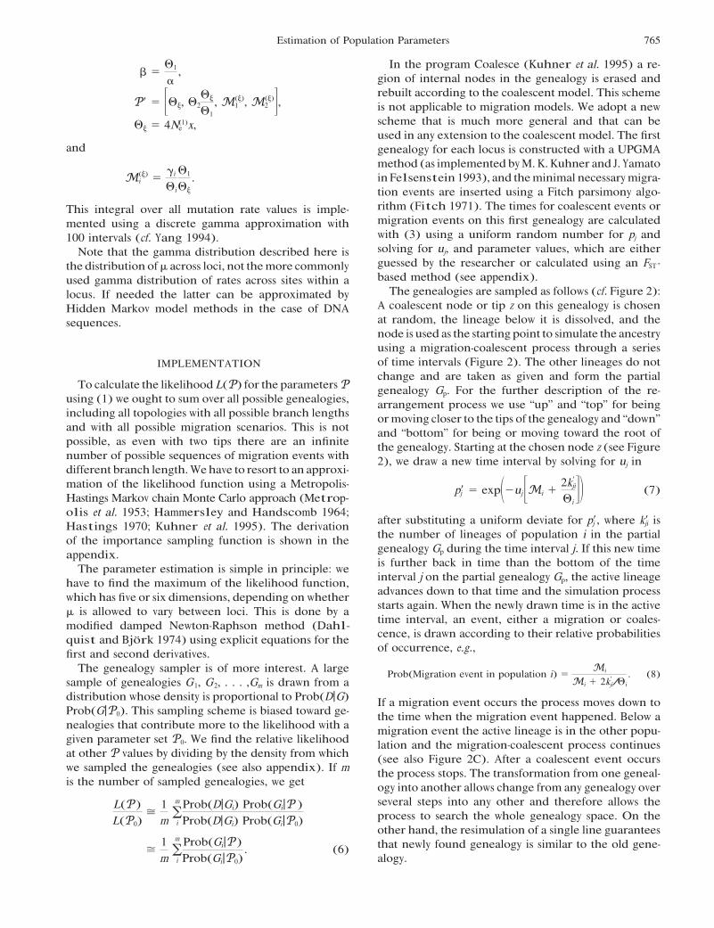
The genealogies are sampled as follows (cf. Figure 2):locus. If needed the latter can be approximated byA coalescent node or tip z on this genealogy is chosenHidden Markov model methods in the case of DNAat random, the lineage below it is dissolved, and thesequences.node isused as the starting point to simulate the ancestryusing a migration-coalescent process through a seriesof time intervals (Figure 2). The other lineages do notIMPLEMENTATIONchange and are taken as given and form the partial

To calculate the likelihood L(P) for the parametersP genealogy Gp. For the further description of the re-using (1) we ought to sum over all possible genealogies, arrangement process we use “up” and “top” for beingincluding all topologies with all possible branch lengths ormoving closer to the tips of the genealogy and “down”and with all possible migration scenarios. This is not and “bottom” for being or moving toward the root ofpossible, as even with two tips there are an infinite the genealogy. Starting at the chosen node z (see Figurenumber of possible sequences of migration events with 2), we draw a new time interval by solving for uj indifferent branch length.We have to resort to an approxi-mation of the likelihood function using a Metropolis- p,j " exp"$uj #Mi %

2k,ji

#i$% (7)

Hastings Markov chain Monte Carlo approach (Metrop-olis et al. 1953; Hammersley and Handscomb 1964;

after substituting a uniform deviate for p,j , where k,ji isHastings 1970; Kuhner et al. 1995). The derivationthe number of lineages of population i in the partialof the importance sampling function is shown in thegenealogy Gp during the time interval j. If this new timeappendix.is further back in time than the bottom of the timeThe parameter estimation is simple in principle: weinterval j on the partial genealogy Gp, the active lineagehave to find the maximum of the likelihood function,advances down to that time and the simulation processwhich has five or six dimensions, depending on whetherstarts again. When the newly drawn time is in the active

& is allowed to vary between loci. This is done by atime interval, an event, either a migration or coales-modified damped Newton-Raphson method (Dahl-cence, is drawn according to their relative probabilitiesquist and Bjork 1974) using explicit equations for theof occurrence, e.g.,first and second derivatives.

The genealogy sampler is of more interest. A large Prob(Migration event in population i) "Mi

Mi % 2k,ji/#i

. (8)sample of genealogies G 1, G 2, . . . ,Gm is drawn from adistribution whose density is proportional to Prob(D|G) If a migration event occurs the process moves down toProb(G|P0). This sampling scheme is biased toward ge- the time when the migration event happened. Below anealogies that contribute more to the likelihood with a migration event the active lineage is in the other popu-given parameter set P0. We find the relative likelihood lation and the migration-coalescent process continuesat other P values by dividing by the density from which (see also Figure 2C). After a coalescent event occurswe sampled the genealogies (see also appendix). If m the process stops. The transformation from one geneal-is the number of sampled genealogies, we get ogy into another allows change from any genealogy over

several steps into any other and therefore allows theL(P)L(P0)

( 1m &

m

i

Prob(D|Gi) Prob(Gi|P )Prob(D|Gi) Prob(Gi|P0) process to search the whole genealogy space. On the

other hand, the resimulation of a single line guaranteesthat newly found genealogy is similar to the old gene-( 1

m &m

i

Prob(Gi|P)Prob(Gi|P0)

. (6)alogy.


Figure 2.—Transitionfrom an old genealogy Go toa new genealogy Gn. Dottedlines are the times of coales-cences or migrations. (A)Genealogy Go with migra-tion. The black bar marksa migration from the whitepopulation to the black orvice versa; z is the node tobe picked. (B) Partial gene-alogy Gp after drawing thecoalescent node z at ran-dom and dissolving thebranch to the next coales-cent below. (C) Simulationof the coalescent with mi-gration. One possible out-come with three consecu-tive steps is shown: (1) usingEquation 7 a new time inter-val is drawn and a migrationevent from white to black isalso drawn (Equation 8)and the lineage is extendeddown to that event; (2) anew time interval is drawn:it extends too far back, sothe lineage advances downto the time j; (3) a new timeinterval is drawn with a coa-lescent event at its bottomend. The process stops attime k. (D) the final con-figuration Gn.

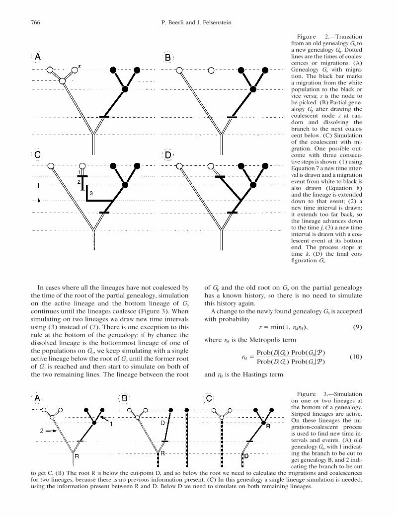
In cases where all the lineages have not coalesced by of Gp and the old root on Go on the partial genealogyhas a known history, so there is no need to simulatethe time of the root of the partial genealogy, simulation

on the active lineage and the bottom lineage of Gp this history again.A change to the newly found genealogy Gn is acceptedcontinues until the lineages coalesce (Figure 3). When

simulating on two lineages we draw new time intervals with probabilityr " min(1, rMrH), (9)using (3) instead of (7). There is one exception to this

rule at the bottom of the genealogy: if by chance thewhere rM is the Metropolis termdissolved lineage is the bottommost lineage of one of

the populations on Go, we keep simulating with a singlerM "

Prob(D|Gn) Prob(Gn|P)Prob(D|Go) Prob(Go|P)

(10)active lineage below the root of Gp until the former rootof Go is reached and then start to simulate on both ofthe two remaining lines. The lineage between the root and rH is the Hastings term

Figure 3.—Simulationon one or two lineages atthe bottom of a genealogy.Striped lineages are active.On these lineages the mi-gration-coalescent processis used to find new time in-tervals and events. (A) oldgenealogyGo, with 1 indicat-ing the branch to be cut toget genealogy B, and 2 indi-cating the branch to be cut

to get C. (B) The root R is below the cut-point D, and so below the root we need to calculate the migrations and coalescencesfor two lineages, because there is no previous information present. (C) In this genealogy a single lineage simulation is needed,using the information present between R and D. Below D we need to simulate on both remaining lineages.


with the biggest contribution to the likelihood andrH "

Prob(Go|Gn)Prob(Gn|Go)

. (11) therefore approximate the maximum-likelihood esti-mate of our parameters P. The main problem with

This acceptance probability r is based on the work of importance sampling schemes is that little is knownHastings (1970). In our specific implementation it can about how we can be sure that we have sampled enoughbe simplified. The scheme for changing the genealogy genealogies from the region that contributes most tocreates a new genealogy from an old one by first ran- our likelihood function. It is common practice in ourdomly removing a branch with all its possible migration group to run 10 “short” chains and then 2 “long” chains.events, which creates a partial genealogy Gp. The proba- Using random values for the first parameter set, we havebility of a particular change is only governed by the found that for a given data set the results converge tonumber of coalescent nodes in the genealogy, and this a value that is not dependent on these initial parameternumber is constant so that the probabilities Prob(Gp|Gn) values when the total numbers of sampled genealogiesand Prob(Gp|Go) are equal. For a specific triplet of origi- exceed 30,000 genealogies (data not shown). These arenal, partial, and new genealogies Go, Gp, and Gn 10 short chains with 1000 genealogies and 2 long chains

with 10,000 genealogies sampled. It seems to be suffi-Prob(Gn|Go) " Prob(Gp|Go) Prob(Gn|Gp) (12)cient to deliver acceptable estimates for simulated data

holds. The resimulation process (7)–(8) is driven only and averages of those, although we would recommendby the parameters P and so Prob(G|Gp) is proportional choosing a better start parameter than a random guessto Prob(G|P) so that and running the program at least twice as long. The

number of genealogies needed for an accurate estimaterH "

Prob(Gp|Gn) Prob(Go|Gp)Prob(Gp|Go) Prob(Gn|Gp)

is certainly dependent on many factors, such as startingparameters, first genealogy, number of sampled individ-

"Prob(Go|P)Prob(Gn|P)

. (13)TABLE 1

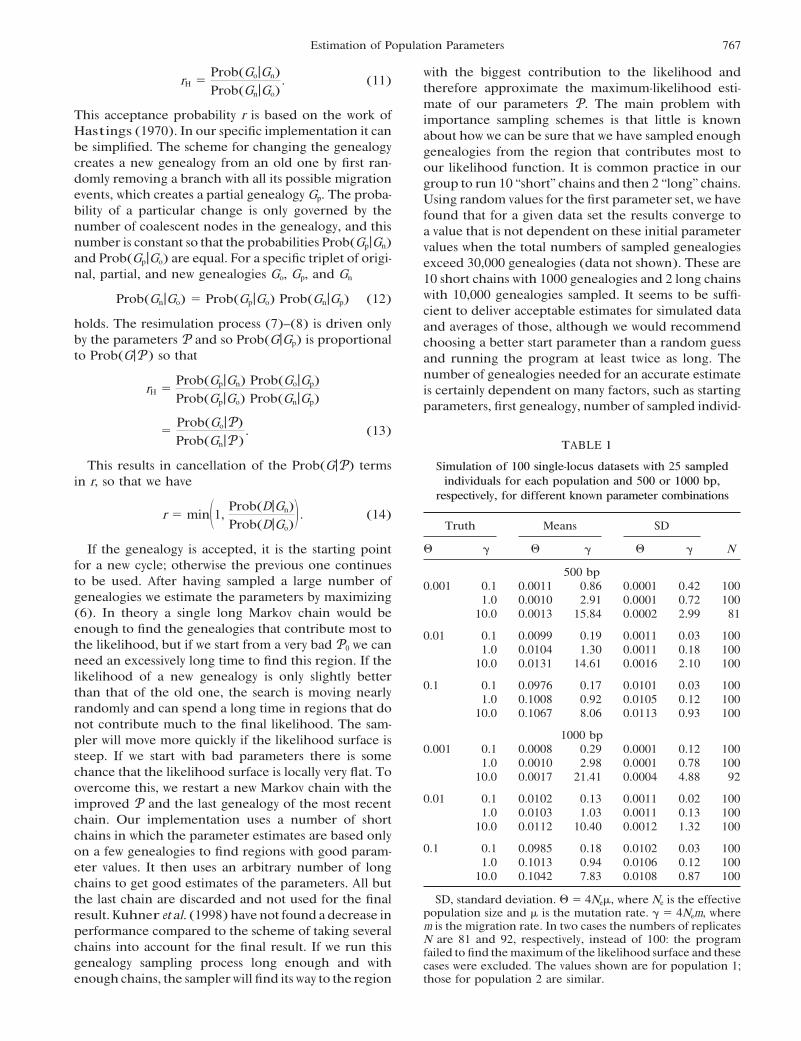
This results in cancellation of the Prob(G|P) terms Simulation of 100 single-locus datasets with 25 sampledindividuals for each population and 500 or 1000 bp,in r, so that we have

respectively, for different known parameter combinations

r " min"1,Prob(D|Gn)Prob(D|Go)

% . (14)Truth Means SD

# ! # ! # ! NIf the genealogy is accepted, it is the starting pointfor a new cycle; otherwise the previous one continues 500 bpto be used. After having sampled a large number of 0.001 0.1 0.0011 0.86 0.0001 0.42 100genealogies we estimate the parameters by maximizing 1.0 0.0010 2.91 0.0001 0.72 100(6). In theory a single long Markov chain would be 10.0 0.0013 15.84 0.0002 2.99 81enough to find the genealogies that contribute most to 0.01 0.1 0.0099 0.19 0.0011 0.03 100the likelihood, but if we start from a very bad P0 we can 1.0 0.0104 1.30 0.0011 0.18 100need an excessively long time to find this region. If the 10.0 0.0131 14.61 0.0016 2.10 100likelihood of a new genealogy is only slightly better

0.1 0.1 0.0976 0.17 0.0101 0.03 100than that of the old one, the search is moving nearly 1.0 0.1008 0.92 0.0105 0.12 100randomly and can spend a long time in regions that do 10.0 0.1067 8.06 0.0113 0.93 100not contribute much to the final likelihood. The sam-

1000 bppler will move more quickly if the likelihood surface is0.001 0.1 0.0008 0.29 0.0001 0.12 100steep. If we start with bad parameters there is some 1.0 0.0010 2.98 0.0001 0.78 100

chance that the likelihood surface is locally very flat. To 10.0 0.0017 21.41 0.0004 4.88 92overcome this, we restart a new Markov chain with the

0.01 0.1 0.0102 0.13 0.0011 0.02 100improved P and the last genealogy of the most recent1.0 0.0103 1.03 0.0011 0.13 100chain. Our implementation uses a number of short 10.0 0.0112 10.40 0.0012 1.32 100

chains in which the parameter estimates are based only0.1 0.1 0.0985 0.18 0.0102 0.03 100on a few genealogies to find regions with good param-

1.0 0.1013 0.94 0.0106 0.12 100eter values. It then uses an arbitrary number of long10.0 0.1042 7.83 0.0108 0.87 100chains to get good estimates of the parameters. All but

SD, standard deviation. # " 4Ne&, where Ne is the effectivethe last chain are discarded and not used for the finalpopulation size and & is the mutation rate. ! " 4Nem, whereresult.Kuhner et al. (1998) have not found a decrease inm is the migration rate. In two cases the numbers of replicatesperformance compared to the scheme of taking severalN are 81 and 92, respectively, instead of 100: the program

chains into account for the final result. If we run this failed to find the maximum of the likelihood surface and thesegenealogy sampling process long enough and with cases were excluded. The values shown are for population 1;

those for population 2 are similar.enough chains, the samplerwill find its way to the region


TABLE 2

Influence of number of sites and number of loci on parameter estimates

Loci

1 2 5 10[100] [50] [20] [10]

bp # ! # ! # ! # !

Means500 0.0102 1.13 0.0088 1.06 0.0097 0.99 0.0108 0.97

1,000 0.0098 1.05 0.0104 1.10 0.0104 1.16 0.0100 0.772,000 0.0107 0.99 0.0098 1.02 0.0104 1.00 0.0100 0.835,000 0.0103 0.96 0.0103 0.90 0.0104 0.87 0.0107 0.89

10,000 0.0102 0.88 0.0103 0.89 0.0100 0.82 0.0109 0.83

Standard deviations500 0.0011 0.17 0.013 0.19 0.0023 0.25 0.0036 0.34

1,000 0.0010 0.13 0.0015 0.20 0.0024 0.28 0.0034 0.262,000 0.0011 0.13 0.0014 0.18 0.0024 0.25 0.0034 0.295,000 0.0011 0.12 0.0015 0.15 0.0024 0.21 0.0036 0.31

10,000 0.0011 0.11 0.0015 0.14 0.0023 0.19 0.0037 0.29

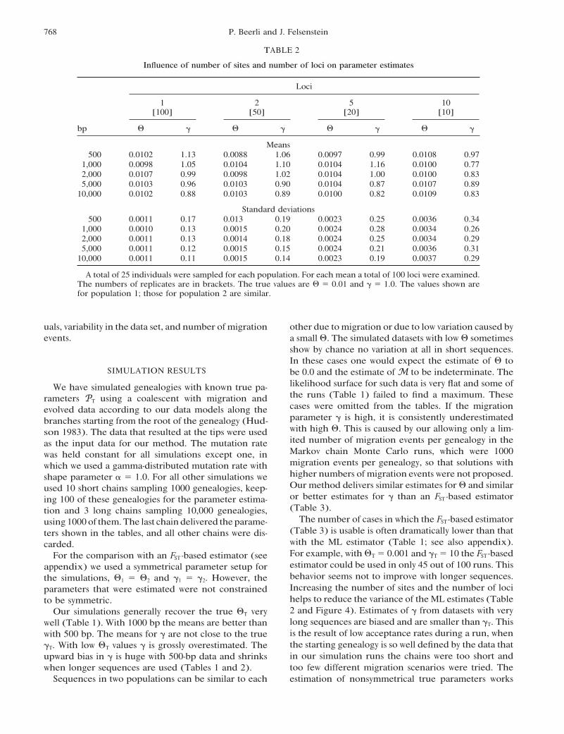
A total of 25 individuals were sampled for each population. For each mean a total of 100 loci were examined.The numbers of replicates are in brackets. The true values are # " 0.01 and ! " 1.0. The values shown arefor population 1; those for population 2 are similar.

uals, variability in the data set, and number ofmigration other due to migration or due to low variation caused byevents. a small #. The simulated datasets with low # sometimes

show by chance no variation at all in short sequences.In these cases one would expect the estimate of # to

SIMULATION RESULTS be 0.0 and the estimate of M to be indeterminate. Thelikelihood surface for such data is very flat and some ofWe have simulated genealogies with known true pa-the runs (Table 1) failed to find a maximum. Theserameters PT using a coalescent with migration andcases were omitted from the tables. If the migrationevolved data according to our data models along theparameter ! is high, it is consistently underestimatedbranches starting from the root of the genealogy (Hud-with high #. This is caused by our allowing only a lim-son 1983). The data that resulted at the tips were usedited number of migration events per genealogy in theas the input data for our method. The mutation rateMarkov chain Monte Carlo runs, which were 1000was held constant for all simulations except one, inmigration events per genealogy, so that solutions withwhich we used a gamma-distributed mutation rate withhigher numbers ofmigration events were not proposed.shape parameter ' " 1.0. For all other simulations weOur method delivers similar estimates for # and similarused 10 short chains sampling 1000 genealogies, keep-or better estimates for ! than an FST -based estimatoring 100 of these genealogies for the parameter estima-(Table 3).tion and 3 long chains sampling 10,000 genealogies,

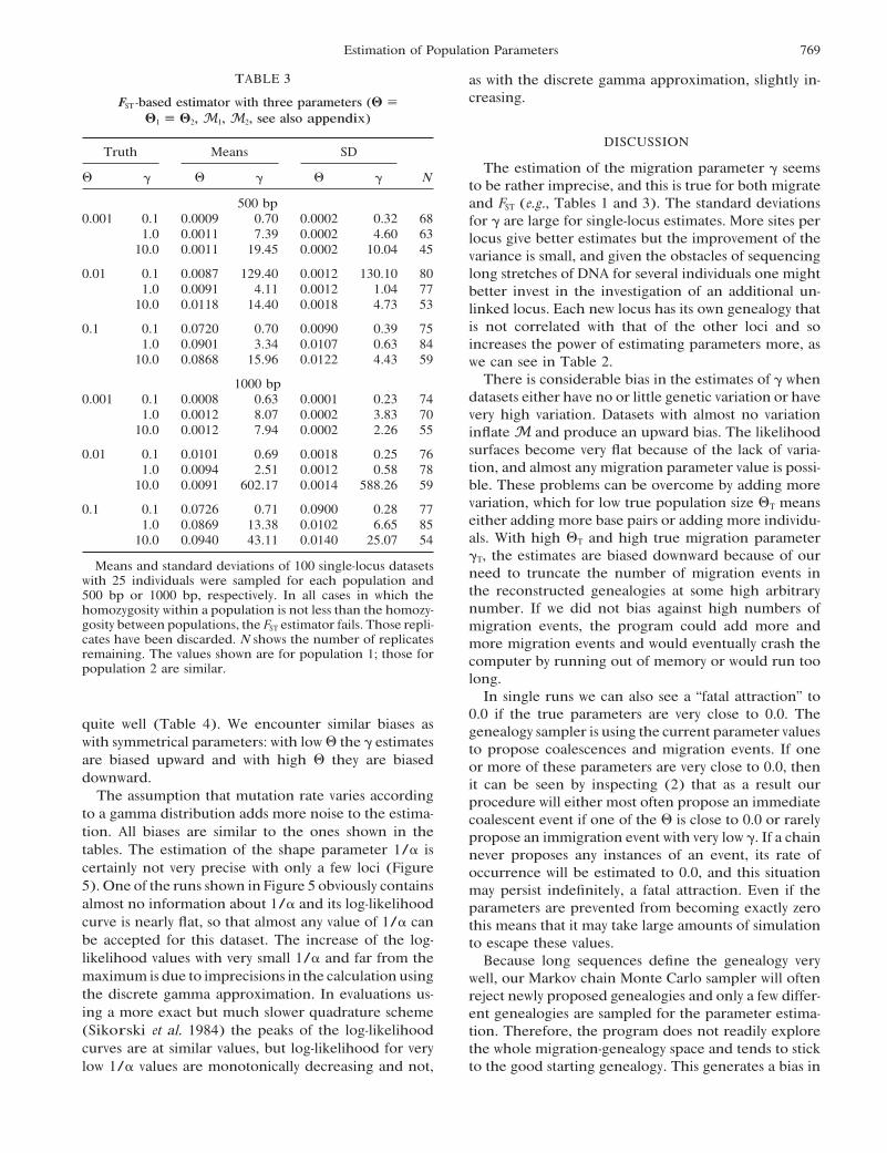
The number of cases in which the FST -based estimatorusing 1000 of them.The last chain delivered the parame-(Table 3) is usable is often dramatically lower than thatters shown in the tables, and all other chains were dis-with the ML estimator (Table 1; see also appendix).carded.For example, with #T " 0.001 and !T " 10 the FST -basedFor the comparison with an FST -based estimator (seeestimator could be used in only 45 out of 100 runs. Thisappendix) we used a symmetrical parameter setup forbehavior seems not to improve with longer sequences.the simulations, #1 " #2 and !1 " !2. However, theIncreasing the number of sites and the number of lociparameters that were estimated were not constrainedhelps to reduce the variance of the ML estimates (Tableto be symmetric.2 and Figure 4). Estimates of ! from datasets with veryOur simulations generally recover the true #T verylong sequences are biased and are smaller than !T. Thiswell (Table 1). With 1000 bp the means are better thanis the result of low acceptance rates during a run, whenwith 500 bp. The means for ! are not close to the truethe starting genealogy is so well defined by the data that!T. With low #T values ! is grossly overestimated. Thein our simulation runs the chains were too short andupward bias in ! is huge with 500-bp data and shrinkstoo few different migration scenarios were tried. Thewhen longer sequences are used (Tables 1 and 2).

Sequences in two populations can be similar to each estimation of nonsymmetrical true parameters works


TABLE 3 as with the discrete gamma approximation, slightly in-creasing.FST -based estimator with three parameters (! )

!1 ) !2, M1, M2, see also appendix)

DISCUSSIONTruth Means SD

The estimation of the migration parameter ! seems# ! # ! # ! N to be rather imprecise, and this is true for both migrate

500 bp and FST (e.g., Tables 1 and 3). The standard deviations0.001 0.1 0.0009 0.70 0.0002 0.32 68 for ! are large for single-locus estimates. More sites per

1.0 0.0011 7.39 0.0002 4.60 63 locus give better estimates but the improvement of the10.0 0.0011 19.45 0.0002 10.04 45 variance is small, and given the obstacles of sequencing

0.01 0.1 0.0087 129.40 0.0012 130.10 80 long stretches of DNA for several individuals one might1.0 0.0091 4.11 0.0012 1.04 77 better invest in the investigation of an additional un-

10.0 0.0118 14.40 0.0018 4.73 53 linked locus. Each new locus has its own genealogy thatis not correlated with that of the other loci and so0.1 0.1 0.0720 0.70 0.0090 0.39 75

1.0 0.0901 3.34 0.0107 0.63 84 increases the power of estimating parameters more, as10.0 0.0868 15.96 0.0122 4.43 59 we can see in Table 2.

There is considerable bias in the estimates of ! when1000 bpdatasets either have no or little genetic variation or have0.001 0.1 0.0008 0.63 0.0001 0.23 74

1.0 0.0012 8.07 0.0002 3.83 70 very high variation. Datasets with almost no variation10.0 0.0012 7.94 0.0002 2.26 55 inflate M and produce an upward bias. The likelihood

surfaces become very flat because of the lack of varia-0.01 0.1 0.0101 0.69 0.0018 0.25 76tion, and almost any migration parameter value is possi-1.0 0.0094 2.51 0.0012 0.58 78

10.0 0.0091 602.17 0.0014 588.26 59 ble. These problems can be overcome by adding morevariation, which for low true population size #T means0.1 0.1 0.0726 0.71 0.0900 0.28 77either adding more base pairs or adding more individu-1.0 0.0869 13.38 0.0102 6.65 85als. With high #T and high true migration parameter10.0 0.0940 43.11 0.0140 25.07 54!T, the estimates are biased downward because of our

Means and standard deviations of 100 single-locus datasets need to truncate the number of migration events inwith 25 individuals were sampled for each population andthe reconstructed genealogies at some high arbitrary500 bp or 1000 bp, respectively. In all cases in which thenumber. If we did not bias against high numbers ofhomozygosity within a population is not less than the homozy-

gosity between populations, the FST estimator fails. Those repli- migration events, the program could add more andcates have been discarded. N shows the number of replicates more migration events and would eventually crash theremaining. The values shown are for population 1; those for computer by running out of memory or would run toopopulation 2 are similar.

long.In single runs we can also see a “fatal attraction” to

0.0 if the true parameters are very close to 0.0. Thequite well (Table 4). We encounter similar biases as genealogy sampler is using the current parameter valueswith symmetrical parameters: with low # the ! estimates to propose coalescences and migration events. If oneare biased upward and with high # they are biased or more of these parameters are very close to 0.0, thendownward. it can be seen by inspecting (2) that as a result our

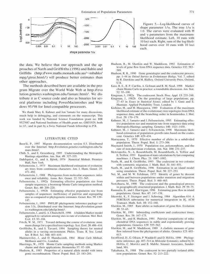
The assumption that mutation rate varies according procedure will either most often propose an immediateto a gamma distribution adds more noise to the estima- coalescent event if one of the # is close to 0.0 or rarelytion. All biases are similar to the ones shown in the propose an immigration event with very low !. If a chaintables. The estimation of the shape parameter 1/' is never proposes any instances of an event, its rate ofcertainly not very precise with only a few loci (Figure occurrence will be estimated to 0.0, and this situation5). One of the runs shown in Figure 5 obviously contains may persist indefinitely, a fatal attraction. Even if thealmost no information about 1/' and its log-likelihood parameters are prevented from becoming exactly zerocurve is nearly flat, so that almost any value of 1/' can this means that it may take large amounts of simulationbe accepted for this dataset. The increase of the log- to escape these values.likelihood values with very small 1/' and far from the Because long sequences define the genealogy verymaximum is due to imprecisions in the calculation using well, our Markov chain Monte Carlo sampler will oftenthe discrete gamma approximation. In evaluations us- reject newly proposed genealogies and only a few differ-ing a more exact but much slower quadrature scheme ent genealogies are sampled for the parameter estima-(Sikorski et al. 1984) the peaks of the log-likelihood tion. Therefore, the program does not readily explorecurves are at similar values, but log-likelihood for very the whole migration-genealogy space and tends to stick

to the good starting genealogy. This generates a bias inlow 1/' values are monotonically decreasing and not,


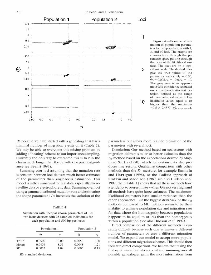
Figure 4.—Example of esti-mation of population parame-ters for two populations with 1,3, and 10 loci. The graphs arecross-sections through the pa-rameter space passing throughthe peak of the likelihood sur-face. The axes are on a loga-rithmic scale. The dashed linesgive the true values of theparameter values: #1 " 0.05,#2 " 0.005, !1 " 10.0, !2 " 1.0.The gray area is an approxi-mate 95% confidence set basedon a likelihood-ratio test cri-terion defined as the rangeof parameter values with log-likelihood values equal to orhigher than the maximum$0.5 - 9.4877 (.2

d.f. " 4; ' " 0.05).

M because we have started with a genealogy that has a parameters but allows more realistic estimation of theparameters with several loci.minimal number of migration events on it (Table 2).

We may be able to overcome this mixing problem by Conclusion: Our method based on coalescents withmigration delivers similar or better estimates than theadding a “heating” scheme to our importance sampling.

Currently the only way to overcome this is to run the FST method based on the expectations derived by May-nard Smith (1970), which for certain data also pro-chainsmuch longer than the defaults (forpractical guid-

ance see Beerli 1997). duces fine results. Qualitative comparison with othermethods than the FST measure, for example RannalaSumming over loci assuming that the mutation rate

is constant between loci delivers much better estimates and Hartigan (1996), or the cladistic approach ofSlatkin and Maddison (1989; see also Hudson et al.of the parameters than single-locus estimation. This

model is rather unnatural for real data, especially micro- 1992, their Table 1) shows that all these methods havea tendency to overestimate ! when # isnot veryhigh andsatellite data or electrophoretic data. Summing over loci

using a gamma-distributedmutation rate and estimating all methods have quite large variances. The maximum-likelihood estimators have smaller variances than thethe shape parameter 1/' increases the variation of theother approaches. But the biggest drawback of the FST

methods compared to ML methods seems to be theirTABLE 4 inability to estimate population size and migration rate

for data where the homozygosity between populationsSimulation with unequal known parameters of 100two-locus datasets with 25 sampled individuals for happens to be equal to or less than the homozygosity

each population and 500 bp per locus within a population (see also Hudson et al. 1992).Direct comparison of the different methods is cur-

Population 1 Population 2 rently difficult because each one estimates a differentnumber of parameters or uses a different migration# ! # !model. We expand our model to accept more popula-

Truth 0.0500 10.00 0.0050 1.00 tions and differentmigration schemes. This should thenMeans 0.0476 8.35 0.0048 1.21 facilitate direct comparison. We believe that taking theSD 0.0052 1.09 0.0005 0.15 history of mutation into account and summing over all

SD, standard deviation. possible genealogies gains the most information from


Figure 5.—Log-likelihood curves ofshape parameter 1/'. The true 1/' is1.0. The curves were evaluated with #and ! parameters from the maximum-likelihood estimate. Left, 10 runs with10 loci each. Right, sum of the log-likeli-hood curves over 10 runs with 10 locieach.

Hudson, R., M. Slatkin and W. Maddison, 1992 Estimation ofthe data. We believe that our approach and the ap-levels of gene flow from DNA sequence data. Genetics 132: 583–

proaches ofNath andGriffiths (1996) and Bahlo and 589.Hudson, R. R., 1990 Gene genealogies and the coalescent process,Griffiths (http://www.maths.monash.edu.au/!mbahlo/

pp. 1–44 in Oxford Surveys in Evolutionary Biology, Vol. 7, editedmpg/gtree.html/) will produce better estimates thanby R. Dawkins and M. Ridley. Oxford University Press, Oxford,

other approaches. U.K.Kass, R. E., B. P. Carlin, A. Gelman and R. M. Neal, 1998 MarkovThe methods described here are available in the pro-

chain Monte Carlo in practice: a roundtable discussion. Am. Stat.gram Migrate over the World Wide Web at http://evo52: 93–100.

lution.genetics.washington.edu/lamarc.html/. We dis- Kingman, J., 1982a The coalescent. Stoch. Proc. Appl. 13: 235–248.Kingman, J., 1982b On the genealogy of large populations, pp.tribute it as C source code and also as binaries for sev-

27–43 in Essays in Statistical Science, edited by J. Gani and E.eral platforms including PowerMacintoshes and Win-Hannan. Applied Probability Trust, London.

dows 95/98 for Intel-compatible processors. Kishino, H., and M. Hasegawa, 1989 Evaluation of the maximumlikelihood estimate of the evolutionary tree topologies from DNAWe thank Mary K. Kuhner and Jon Yamato for many discussions,sequence data, and the branching order in hominoidea. J. Mol.much help in debugging, and comments on the manuscript. ThisEvol. 29: 170–179.

work was funded by National Science Foundation grant no. BIR Kuhner, M., J. Yamato and J. Felsenstein, 1995 Estimating effec-9527687 and National Institutes of Health grant no. GM51929, both tive population size and mutation rate from sequence data usingto J.F., and in part by a Swiss National Funds fellowship to P.B. Metropolis-Hastings sampling. Genetics 140: 1421–1430.

Kuhner, M., J. Yamato and J. Felsenstein, 1998 Maximum likeli-hood estimation of population growth rates based on the coales-cent. Genetics 149: 429–434.

LITERATURE CITED Maruyama, T., 1970 Effective number of alleles in a subdividedpopulation. Theor. Popul. Biol. 1: 273–306.Beerli, P., 1997 Migrate documentation version 0.3. Distributed

Maynard Smith, J., 1970 Population size, polymorphism, and theover the Internet: http://evolution.genetics.washington.edu/la-rate of non-darwinian evolution. Am. Nat. 104: 231–237.marc.html/.

Metropolis, N., A. Rosenbluth, M. Rosenbluth, A. Teller andChib, S., and E. Greenberg, 1995 Understanding the Metropolis-E.Teller, 1953 Equation of state calculationsby fast computingHastings algorithm. Am. Stat. 49: 327–335.machines. J. Chem. Phys. 21: 1087–1092.Dahlquist, G., and A. Bjork, 1974 Numerical Methods. Prentice-

Nath, H., and R. Griffiths, 1993 The coalescent in two coloniesHall, New York.with symmetric migration. J. Math. Biol. 31: 841–851.Felsenstein, J., 1973 Maximum likelihood estimation of evolution-

Nath, H., and R. Griffiths, 1996 Estimation in an island modelary trees from continuous characters. Am. J. Hum. Genet. 25:using simulation. Theor. Popul. Biol. 50: 227–253.471–492.

Nei, M., and M. W. Feldman, 1972 Identity of genes by descentFelsenstein, J., 1988 Phylogenies from molecular sequences: infer-within and between populations under mutation and migrationence and reliability. Annu. Rev. Genet. 22: 521–565.pressures. Theor. Popul. Biol. 3: 460–465.Felsenstein, J., 1992a Estimating effective population size from

Notohara, M., 1990 The coalescent and the genealogical processsample sequences: a bootstrap Monte Carlo integration method.in geographically structured population. J. Math. Biol. 29: 59–75.Genet. Res. 60: 209–220.

Rannala, B., and J. Hartigan, 1996 Estimating gene flow in islandFelsenstein, J., 1992b Estimating effective population size frompopulations. Genet. Res. 67: 147–158.samples of sequences: inefficiency of pairwise and segregating

Sikorski, K., F. Stenger and J. Schwing, 1984 Algorithm 614: Asites as compared to phylogenetic estimates. Genet. Res. 59: 139–FORTRAN subroutine for numerical integration in Hp. ACM147.Transact. Math. Soft. 10: 152–160.Felsenstein, J., 1993 PHYLIP: phylogenetic inference package ver-

Slatkin, M., 1985 Rare alleles as indicators of gene flow. Evolutionsion 3.5c. Distributed over the Internet: http://evolution.genet-39: 53–65.ics.washington.edu/phylip.html/.

Slatkin, M., 1991 Inbreeding coefficients and coalescence times.Felsenstein, J., andG.A.Churchill, 1996 AhiddenMarkovmodelGenet. Res. 58: 167–175.approach to variation among sites in rate of evolution. Mol. Biol.

Slatkin, M., and R. Hudson, 1991 Pairwise comparisons of mito-Evol. 13: 93–104.chondrial DNA sequences in stable and exponentially growingFitch, W. M., 1971 Toward defining the course of evolution: mini-populations. Genetics 129: 555–562.mumchange for a specified tree topology. Syst.Zool. 20: 406–416.

Slatkin, M., and W. Maddison, 1989 A cladistic measure of geneGriffiths, R., and S. Tavare, 1994 Sampling theory for neutralflow inferred from the phylogenies of alleles. Genetics 123: 603–alleles in a varying environment. Philos. Trans. R. Soc. Lond.613.Ser. B Biol. Sci. 344: 403–410.

Swofford, D., G. Olsen, P. Waddell and D. Hillis, 1996 Phyloge-Hammersley, J., and D. Handscomb, 1964 Monte Carlo Methods.netic inference, pp. 407–514 in Molecular Systematics, edited by D.Methuen and Co., London.Hillis, C. Moritz and B. Mable. Sinauer Associates, Sunder-Hastings, W., 1970 Monte Carlo sampling methods using Markovland, MA.chains and their applications. Biometrika 57: 97–109.

Takahata, N., 1988 The coalescent in two partially isolated diffu-Hudson, R., 1983 Properties of a natural allele model with intra-genic recombination. Theor. Popul. Biol. 23: 183–201. sion populations. Genet. Res. 52: 213–222.


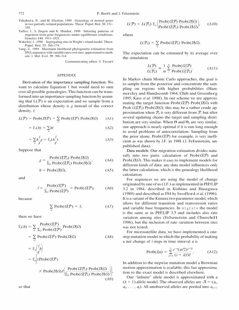
Takahata, N., and M. Slatkin, 1990 Genealogy of neutral genesin two partially isolated populations. Theor. Popul. Biol. 38: 331– L(P) " L(P0) !g "Prob(G|P) Prob(D|G)

Prob(G|P0) Prob(D|G)%, (A10)350.

Tufto, J., S. Engen and K. Hindar, 1996 Inferring patterns ofmigration from gene frequencies under equilibrium conditions. whereGenetics 144: 1911–1921.

Wakeley, J., 1998 Segregating sites inWright’s island model. Theor. L(P0) " &G

Prob(G|P0) Prob(D|G).Popul. Biol. 53: 166–174.

Yang, Z., 1994 Maximum likelihood phylogenetic estimation fromDNA sequences with variable rates over sites: approximativemeth- The expectation can be estimated by its average overods. J. Mol. Evol. 39: 306–314. the simulation

Communicating editor: S. TavareL(P)L(P0)

( 1m &

m

i

Prob(Gi|P)Prob(Gi|P0)

. (A11)

APPENDIXIn Markov chain Monte Carlo approaches, the goal is

Derivation of the importance sampling function: We to sample from the posterior and concentrate the sam-want to calculate Equation 1 but would need to sum pling on regions with higher probabilities (Ham-over all possible genealogies. This function can be trans- mersley and Handscomb 1964; Chib and Greenbergformed into an importance sampling function by assum- 1995; Kass et al. 1998). In our scheme we are approxi-ing that L(P) is an expectation and we sample from a mating the target function Prob(G|P) Prob(D|G) withdistribution whose density is g instead of the correct Prob (G|P0) Prob(D|G); this may be a rather crude ap-density, f, proximation when P0 is very different from P, but after

several updating chains the target and sampling distri-L(P) " Prob(D|P) " &G

Prob(G|P) Prob(D|G) (A1)bution are very similar. When # and #0 are very similar,our approach is nearly optimal if it is run long enough" !f(h) " &

Ghf (A2)

to avoid problems of autocorrelation. Sampling fromthe prior alone, Prob(G|P) for example, is very ineffi-

" &Ghfgg " !g(h

fg). (A3) cient as was shown by J.F. in 1988 (J. Felsenstein, un-

published data).Suppose that Data models: Our migration estimation divides natu-

rally into two parts: calculation of Prob(G|P) andg "

Prob(G|P0) Prob(D|G)RG Prob(G|P0) Prob(D|G)

, (A4) Prob(D|G). This makes it easy to implement models fordifferent kinds of data: any data model influences onlythe latter calculation, which is the genealogy likelihoodh " Prob(D|G), (A5)calculation.

and For sequences we are using the model of changeoriginated by one ofus (J.F.) as implemented inPHYLIP

f "Prob(G|P)

RG Prob(G|P)" Prob(G|P), (A6) 3.2 in 1984, described in Kishino and Hasegawa

(1989) and described as F84 by Swofford et al. (1996).It is a variant of the Kimura two-parametermodel, whichbecauseallows for different transition and transversion ratios

&G

Prob(G|P) " 1; (A7) and variable base frequencies. In migrate the modelis the same as in PHYLIP 3.5 and includes also rate

then we have variation among sites (Felsenstein and Churchill1996), but the inclusion of rate variation between sites

!f(h) " &G

Prob(G|P)RG Prob(G|P)

Prob(D|G) was not tested.For microsatellite data, we have implemented a one-

step mutation model in which the probability of making" &G

Prob(G|P) Prob(D|G) (A8)a net change of i steps in time interval u is

" !g "fgh% Prob(i|u) " &∞

k"0

e$u(u/2)i%2k

(i % k)!k!. (A12)

" !g#(Prob(G|P)In addition to the stepwise mutation model a Brownianmotion approximation is available; this fast approxima-

- Prob(D|G)/" Prob(G|P0) Prob(D|G)RG Prob(G|P0) Prob(D|G)%$, tion to the exact model is described elsewhere.

Our “infinite” allele model is approximated with a(A9)(k % 1)-allele model. The observed alleles are A " (a1,a2, . . . , ak). All unobserved alleles are pooled into ak%1.so that


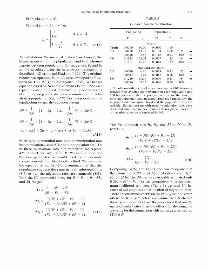
TABLE 5Prob(ai|ai,u) " e$ufai,

FST -based parameter estimationProb(ai|aj,u) " (1 $ e$u)faj,

Population 1 Population 2

# ! # ! Nfaz " *1

k%1if az " A ,

1 $k

k%1if az " A . Means

Truth 0.0500 10.00 0.0050 1.00 —(A13)

SD 0.0138 13.80 0.0138 2.08 25 "

0.0116 3.56 0.0116 0.93 100 #FST calculations: We use a calculation based on F(i)

W , the SM 0.1824 72.04 0.0057 1.25 64 "

homozygosity within the population i and FB, the homo- 0.1167 46.10 0.0048 1.39 100 #

zygosity between populations. For sequences, FW and FB Standard deviationscan be calculated using the heterozygosity calculations SN 0.0029 6.11 0.0029 0.55 25 "described in Slatkin and Hudson (1991). The original 0.0012 1.49 0.0012 0.16 100 #

recurrence equations FW and FB were developed byMay- SM 0.1219 59.01 0.0009 0.21 64 "

nard Smith (1970) and Maruyama (1970). We use an 0.0776 37.55 0.0006 0.19 100 #

equation based on Nei and Feldman (1972). The exactSimulationwith unequal known parameters of 100 two-locusequations are simplified by removing quadratic terms datasets with 25 sampled individuals in each population and

like &2, m2, and &m and divisions by number of individu- 500 bp per locus. SN, the population sizes are the same inals in a population (e.g., m/N). For two populations in both subpopulations and migration rates are variable; SM, the

migration rates are symmetrical and the population sizes areequilibrium we get the equation systemvariable. Simulation runs with negative migration rates werediscarded from the analysis in lines with " signs; in lines withF (1)

W "1

2N1

% "1 $ 2& $ 2m1 $1

2N1% F (1)

W % 2m1FB#, negative values were replaced by 0.0.

F (2)W "

12N2

% "1 $ 2& $ 2m2 $1

2N2% F (2)

W % 2m2FBThe SM approach with #1, #2, and M ) M1 ) M2

results inFB " FB(1 $ 2& $ m1 $ m2) % m1 F (1)W % 2m2F (2)

W ,(A14)

#1 "(1 $ F (1)

W )(F (1)W % F (2)

W $ 2FB

(F (1)W )2 % F (1)

W F (2)W $ 2F 2

Bwhere & is the mutation rate, mi is the immigration rateinto population i, and Ni is the subpopulation size. To

#2 "(1 $ F (2)

W )(F (1)W % F (2)

W $ 2FB)(F (2)

W )2 % F (1)W F (2)

W $ 2F 2B

fit these calculations into our framework we replace4N& with # and m/& with M. We cannot solve forthe four parameters we would need for an accurate M "

2FB

F (1)W % F (2)

W $ 2FB

. (A16)comparison with our likelihood method. We can solvethe equation system (A14) by assuming either that the

Comparing (A15) and (A16) one can recognize thatpopulation sizes are the same in both subpopulationsthe estimation of Mi in (A15) breaks down when FB /(SN) or that the migration rates are symmetric (SM).F (i)

W . In (A16) the M can be reasonably estimated onlyWith the SN approach solving for # ) #1 ) #2, M1,if 2FB 0 F (1)

W % F (2)W . For the comparison with our maxi-and M2 we get

mum-likelihood estimator (Table 3) we used SN be-cause of our emphasis on estimation of migration rates.# "

2 $ F (1)W $ F (2)

W

2FB % F (1)W % F (2)

W

,There are differences between the two FST methods evenwhen the true parameters are symmetrical (data not

M1 "2FBF (1)

W % F (1)W $ F (2)

W $ 2FB

(F (1)W $ FB)(F (1)

W % F (2)W $ 2)

, shown), but we do not have the impression that one FST

method works better than the other over the range weare using for the comparisonwith our migratemethodM2 "

2FBF (2)W % F (2)

W $ F (1)W $ 2FB

(F (2)W $ FB)(F (1)

W % F (2)W $ 2)

. (A15)(Table 5).

Documents

MaximumLikelihood Estimation of Migration ates and