Maximum Mean Discrepancy Imitation LearningBeomjoon Kim

School of Computer ScienceMcGill UniversityMontreal, Canada

Email: bkim43@cs.mcgil.ca

Joelle PineauSchool of Computer Science

McGill UniversityMontreal, Canada

Email: jpineau@cs.mcgill.ca

Abstract—Imitation learning is an efficient method for manyrobots to acquire complex skills. Some recent approaches toimitation learning provide strong theoretical performance guar-antees. However, there remain crucial practical issues, especiallyduring the training phase, where the training strategy mayrequire execution of control policies that are possibly harmfulto the robot or its environment. Moreover, these algorithmsoften require more demonstrations than necessary to achievegood performance in practice. This paper introduces a newapproach called Maximum Mean Discrepancy Imitation Learningthat uses fewer demonstrations and safer exploration policy thanexisting methods, while preserving strong theoretical guaranteeson performance. We demonstrate empirical performance of thismethod for effective navigation control of a social robot ina populated environment, where safety and efficiency duringlearning are primary considerations.

I. INTRODUCTION

Imitation learning is a class of algorithms for efficientlyoptimizing the behaviour of an agent using demonstrationsfrom an expert (or oracle). It is particularly advantageous incomplex robotics tasks, where it can be difficult to specify,or directly learn, a model of the dynamics of the robot andits environment. Imitation learning has been used successfullyin recent years for a large number of robotic tasks, includ-ing helicopter manoeuvring [1], car parking [2], autonomousnavigation [14], and robotic surgery [7].

There are several different methods for imitation learn-ing [4]. The most common approach is to use supervisedlearning to match the actions of the expert, by explicitlyminimizing loss with respect to the demonstration data. How-ever, one important difference between imitation learning andstandard supervised learning is that in imitation learning,the assumption that the data is independent and identicallydistributed (IID) is generally violated, due to the fact that thestate distribution induced by the learned policy is differentfrom that of the oracle. Ignoring this fact means that typicalsupervised approaches to imitation learning may suffer aquadratic loss in the task horizon T [16], rather than havinga loss linear in T as in standard supervised learning tasks.

Recently, an imitation learning algorithm known as DatasetAggregation (DAgger) [17] was proposed, and this workstands out among other imitation learning algorithms for tworeasons. First, the authors showed a reduction from imitationlearning to online learning, thereby opening the door to thisrich literature. The second major contribution was to show that

DAgger has strong theoretical guarantee, and is in fact able toachieve a loss linear in T .

Despite its important insights, DAgger has some drawbacksthat can limit its usefulness in some robotic application.First, we note that in DAgger, as in other imitation learn-ing approaches, the expert’s actions are stored and used forcomputation, but they are not directly executed by the robot.The actions carried-out in the environment are always fromthe robot’s own (partially optimized) policy, and the oracle isnot allowed to intervene. Unfortunately this poses unnecessaryrisk, as the robot could use an exploration policy that is not besafe, carrying out actions that are dangerous, either to itself orits environment. This is particularly problematic in the earlyphases of training, and of particular concern for tasks withhigh-risk states, for example in robot-assisted surgery [7].The second drawback of DAgger for practical deploymentis its naive data aggregation strategy. Since it queries theoracle at every time step and treats each query equally, itcan require large amounts of oracle demonstrations to learnto recover from the mistakes of early policies. Requiring ex-cessive demonstrations from an oracle can be quite expensive,especially if the queries involves highly skilled personnel asin helicopter tasks [1].

The primary contribution of our paper is to propose anew practical imitation learning algorithm to achieve safe andefficient learning in challenging robotic domains. Like DAg-ger, our algorithm iteratively trains policies. Unlike DAgger,however, we propose a query metric that depends on howclose an encountered state is from the distribution of datagathered so far, and query the oracle only if this metric isabove some threshold. To recover faster from mistakes ofpolicies of previous iterations, we aggregate a data point if it isdistributed differently than the datasets gathered so far, and ifthe current policy has made a mistake, and then train a separatepolicy for each distribution of a dataset. As a result, we learnmultiple policies, each specializing in particular regions ofthe state space where previous policies made mistakes, whilefocusing on one particular distribution of data. At a run time,we check which one of the policies is trained with the datasetthat is most closely distributed with the encountered state. Thedistribution discrepancy metric that we employ is MaximumMean Discrepancy (MMD) [10], a criterion that was originallyproposed to determine whether two sets of data are from thesame or different probability distributions.

The other contributions of our paper are to show that ourapproach, Maximum Mean Discrepancy Imitation Learning(MMD-IL), has similar theoretical guarantees as DAgger, aswell as having better empirical performance. We investigateempirical performance of MMD-IL on two contrasting do-mains, one a simulated car driving domain, where we canextensively characterize the performance in terms of efficiency,safety and loss. The second set of experiments is performedusing a mobile robot intended for personal assistance wherewe confirm that MMD-IL can efficiently learn to imitate howan expert drives the robot through a crowd, using significantlyfewer demonstrations than DAgger.

A noteworthy caveat is that the improved safety and dataefficiency observed with MMD-IL is obtained by trading-offdata efficiency with computational efficiency. Indeed, thereis an extra O(m) computational cost (m = # data points)for computing the MMD criteria necessary to choose theagent’s policy1. Therefore the method is particularly intendedfor domains where data is more expensive than computation,which is often the case for imitation learning applications.

II. TECHNICAL BACKGROUND

We denote a state space as S, an action space as A, and apolicy space as Π. Given a task horizon T , the agent followsa policy π : S → A and suffers an immediate loss L(s, a),which we assume bounded in [0, 1]. After taking an action theagent reaches another state s′ with a particular probability.We denote dtπ the state distribution at time t after executingπ from time 1 to t − 1, and dπ = 1

T

∑Tt=1 d

tπ the average

distribution of states over T steps. The expected loss in theseT steps is denoted by J(π) =

∑Tt=1 Es∼dtπ [L(s, π(s)] =

TEs∼dπ [L(s, π(s))]. The demonstration data is defined by thetuple < s, a >, and a trajectory is a sequence of demonstrationdata. The goal in imitation learning is to find a policy π ∈ Πsuch that the policy minimizes J(π). We assume that Π is aclosed, bounded and non-empty convex set in Euclidean space.

A. Imitation via Supervised Learning

The standard approach in imitation learning is to usedemonstration data as supervised learning data, and learn apolicy via regression techniques to map states to actions [4].During a time step t, we collect a training example from theoracle (st, π

∗(st)) where π∗(st) denote action of the oracle atstate st. Since we do not have access to the true loss L(s, a) inimitation learning, we denote l(st, π, π∗) as the surrogate lossof executing policy π at state st with respect to π∗. This canbe any convex loss function, such as squared or hinge loss.We learn a policy by solving:

π̂ = argminπ∈ΠEs∼dπ∗ [l(s, π, π∗)] (1)

One drawback of this simple approach is that it ignoresthe fact that the state distributions of the oracle and thelearner are different. This occurs because when the learnermakes a mistake, the wrong action choice will change the

1This could likely be reduced to a constant by keeping only a fixed set ofpoints, or else reduced to a log factor by using appropriate data structures.

following state distribution such that the states induced are notnecessarily distributed from same distribution as the oracle’straining data. Ross and Bagnell [16] proved that this could leadto a quadratic loss in task horizon, compared to the linear lossthat is observed in standard supervised learning with IID data.

B. Dataset Aggregation

Dataset Aggregation (DAgger) tackles the non-IID problemby iteratively learning a policy [17]. In its simplest form,it proceeds as follows. Let sπ denote a state visited byexecuting π, π∗ the oracle’s policy, and π̂i the policy learnedat iteration i. Initially, the learner is given an oracle datasetD0 = {(sπ∗ , π∗(sπ∗))}, and learns a policy π0 by anysupervised learning method which minimizes the loss of π0

with respect to π∗ at sπ∗ in D0. We execute π0 and collectdata from oracle, D1 = {(sπ0

, π∗(sπ0))}. Policy π1 is learned

from the aggregated dataset, D0 ∪D1. This iterative processof policy execution, data aggregation, and policy optimizationcontinues for N iterations. The purpose of iterative learningis to recover from mistakes of the previous policy. Since thestate distribution is not IID, the learned policy is likely tomake mistakes in regions of the state space that are unfamiliar.Hence by aggregating the oracle’s demonstrations at statesencountered by the previous policy, the hope is that the agentwill learn to recover from those mistakes.

Let Qπ′

t (s, π) denote the t-step loss of executing π in theinitial state and then executing π′. We state here an importanttheorem from Ross and Bagnell [17].

Theorem 1 (from [17]): Let π be such thatEs∼dπ [l(s, π, π∗)] = ε. If Qπ

∗

T−t+1(s, π)−Qπ∗T−t+1(s, π∗) ≤ ufor all action a,t ∈ {1, 2, ..., T}, then J(π) ≤ J(π∗) + uTε.

This theorem basically states that if π has expectedloss of ε in state distribution induced by π, differs from π∗

by one action at time step t, and if the cumulative cost isbounded by u, then the task cost with respect to π∗ is O(uT ).

One of the major contributions of DAgger is its reduction ofimitation learning to no-regret on-line learning. In an on-linelearning problem, the algorithm executes a policy and suffersa loss li(π̂i) at iteration i. The algorithm then modifies itspolicy to produce a new policy, π̂i+1, suffers loss li+1(π̂i+1),and so on. A class of on-line algorithms known as no-regreton-line algorithms guarantees the following:

1

N

N∑i=1

li(πi)−minπ∈Π1

N

N∑i=1

li(π) ≤ δN (2)

where limN→∞δN = 0. If we assume a strongly convex lossfunction, then Follow-The-Leader is a no-regret algorithmwhere in each iteration, it uses the policy that works the bestso far: π̂i+1 = argminπ∈Π

∑ij=1 lj(π) [13]. DAgger can be

seen as a variant of a Follow-The-Leader algorithm in thatit chooses the policy that minimizes the surrogate loss ondata gathered so far. In the reduction of imitation learningto on-line learning, we let li(s, π̂, π∗) = Es∼dπ̂i [l(s, π̂i, π

∗)],

N be the number of training iterations in DAgger, andεN = minπ∈Π

1N

∑Ni=1 li(s, π, π

∗) be the minimum losswe can achieve in the policy space Π in hindsight. Assumel(s, π̂, π∗) is strongly convex and denote π̂1:N the sequenceof learned policies. Then DAgger guarantees the following ifan infinite number of samples per iteration are available:

Theorem 2 (from [17]): For DAgger, if N is O(uT logT )and Qπ

′

T−t+1(s, π) − Qπ′T−t+1(s, π∗) ≤ u then there exists apolicy π ∈ π̂1:N such that J(π) ≤ J(π∗) + uTεN .

The important result here is that DAgger guaranteeslinear loss in terms of the task horizon T .

III. MAX MEAN DISCREPANCY IMITATION LEARNING

The first step towards reducing unsafe and unnecessary ex-ploration is to query the oracle and execute the oracle’s action(i.e. oracle intervention) in cases where the state encounteredis distributed differently from data gathered so far, and thelearner is about to make a mistake. We formally define amistake as the discrepancy between the policy of oracle andthat of the agent:

||π(s)− π∗(s)||1 > γ (3)

where γ is a pre-defined parameter. Note that in the caseof discrete actions, the metric needs to be defined. This alsoreduces the problem of unnecessary exploration in states thatare not reachable in reality, because the oracle is able to directthe learner to states that are reachable in reality. We explainbelow how this is computed and used in our algorithm.

We now introduce the criterion known as Maximum MeanDiscrepancy, which is used as a distance metric to determinewhen to query the expert for demonstration, and which of thepolicies to follow out of multiple policies learned so far.

A. Maximum Mean Discrepancy

Given two sets of data, X := {x1, ..., xm} andY := {y1, ..., yn} drawn IID from p and q respectively,the Maximum Mean Discrepancy criterion determineswhether p = q or p 6= q in reproducing kernel Hilbert space(RKHS).

Definition 1 (from [10]): Let F be a class of functionsf : X → R and let p, q,X, Y be defined as above. ThenMMD and its empirical estimate are defined as:

MMD[F , p, q] := supf∈F (E[f(x)]− E[f(y)])

MMD[F , X, Y ] := supf∈F (1

m

m∑i=1

f(xi)−1

n

n∑i=1

f(yi))

MMD comes with an important theorem which we restatehere.

Theorem 3 (from [10]): Let F be a unit ball in reproducingkernel Hilbert space H, defined on compact metric space X ,with associated kernel k(·, ·). Then MMD[F , p, q] = 0 if

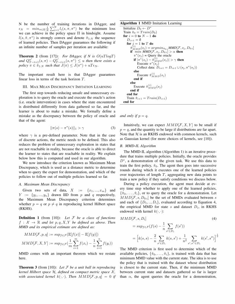
Algorithm 1 MMD Imitation LearningInitialize D0 ← D∗

Train π̂0 = Train(D0)for i = 0 to N − 1 doDi+1 = ∅for j = 1 to T doπ̂

(i)MMD(sj) = argminπ̂0:iMMD[F , sj , D0:i]

if min MMD[F , sj , D0:i] > α thenπ∗(sj) = Query the oracleif |π∗(sj)− π̂(i)

MMD(sj)| > γ thenExecute π∗(sj)Collect data: Di+1 = Di+1 ∪ (s, π

∗(sj))else

Execute π̂(i)MMD(sj)

end ifelse

Execute π̂(i)MMD(sj)

end ifend forTrain π̂i+1 = Train(Di+1)

end for

and only if p = q.

Intuitively, we can expect MMD[F , X, Y ] to be small ifp = q, and the quantity to be large if distributions are far apart.Note that H is an RKHS endowed with common kernels, suchas Gaussian kernel (for more choices of kernels, see [10]).

B. MMD-IL Algorithm

The MMD-IL algorithm (Algorithm 1) is an iterative proce-dure that trains multiple policies. Initially, the oracle providesD∗, a demonstration of the given task. We use this data totrain the first policy, π̂0. The agent then goes into successiverounds during which it executes one of the learned policiesover trajectories of length T , aggregating new data points totrain a new policy if they satisfy conditions we discuss below.

During a policy execution, the agent must decide at ev-ery time step whether to apply one of the learned policies,{π̂0, . . . , π̂i}, or to query the oracle for a demonstration. LetMMD[F , s,D0:i] be the set of MMDs evaluated between sand each of {D1, .., Di}, evaluated according to Equation 4,the empirical MMD for state s and dataset Di, in RKHSendowed with kernel k(·, ·):

MMD[F , s,Di] (4)

= supf∈F (f(s)− 1

n

∑s′∈Di

f(s′))

=[k(s, s)− 2

n

∑s′∈Di

k(s, s′) +1

n2

∑s′,s′′∈Di

k(s′, s′′)] 1

2

The MMD criterion is first used to determine which of theavailable policies, {π̂0, . . . , π̂i}, is trained with data that hasminimum MMD value with the current state. The idea is to usethe policy that is trained with the dataset whose distributionis closest to the current state. Then, if the minimum MMDbetween current state and datasets gathered so far is largerthan α, the agent queries the oracle for a demonstration,

π∗(s). This action gets compared with π̂(i)MMD(s) using the

threshold γ, to decide whether to execute π∗(s) or π̂(i)MMD(s).

If the encountered state has discrepancy bigger than α and thecurrent policy makes a mistake, MMD-IL aggregates the datapoint, (s, π∗(s)). This allows the agent to learn new policiesspecifically targeting unexplored states that are reachable fromcurrent policy and the previous learned policies are stillmaking mistakes, while controlling the frequency of queries.

The MMD-IL algorithm comes with two pre-defined param-eters. The first, γ as introduced above, controls the frequencyof usage of oracle actions. If γ is set to a small value, theoracle’s queried action will be executed and its demonstrationwill be aggregated even for small mistakes. The parameterγ can be set using domain knowledge. Note that we do notexecute the oracle’s action even after it is queried, if thecurrent policy is not making a mistake. This allows the agentto explore states that it will encounter during an execution ofits policy, as long as the policy does not differ from that of theoracle’s. The parameter α, on the other hand, allows the userto control how much the oracle monitoring (i.e. frequency ofqueries to the oracle) is necessary. For instance, if the robot islearning a risk sensitive task, α can be set to 0 in which casethe oracle will provide an action at every step, and the agentuses oracle’s action if the current policy is making a mistake.If α is set to a high value, we only query the oracle when theencountered state is significantly far away from distributionsof data gathered so far. This is more suitable for cases wherethe oracle demonstration data is expensive, and the oracle isnot present with the robot in every step of the policy execution.

C. Space and Time ComplexitiesAssume MMD-IL trained N policies, {π̂1, . . . , π̂N}, from

datasets {D1, .., DN}. In calculating the MMD value betweeneach dataset and the given state, the third term in Eqn 4 ismost expensive to compute, requiring O(m2) time (where mis the number of points in a given dataset Di). But this termcan be pre-computed once Di is fully collected, and so at arun time we only evaluate the second term, which is O(m).Thus, for each query, our algorithm takes O(mN) time, whichcorresponds to the total number of datapoints gathered so far.We also need a O(mN) space to store the data. In practice,this may be reduced in a number of ways, for instance, byimposing a stopping criterion for the number of iterationsbased on MMD values evaluated with new states, or limitingthe number of data points by discarding (near-)duplicate datapoints.D. Theoretical Consequences

In order to prove that our policy is robust, we require aguarantee that our policy achieves a loss linear in T as N getslarge, like supervised learning algorithms[16]. We first assumethat for ith iteration, the oracle interventions have boundedeffect on total variation distance by some constant Ci ≤ 2:

||d(i)πMMD − d

(i)π̂MMD

||1 ≤ Ci

Here, d(i)πMMD denotes the average empirical distribution of

states when the oracle intervened at least once, and d(i)π̂MMD

denotes the average empirical distribution of states when theMMD policy (π̂(i)

MMD) is used throughout the task horizon.We assume that Ci reaches zero as N approaches infinity (i.e.the oracle intervenes less as the number of iterations grows),and the policy at the latest iteration achieves minimumexpected loss out of all the policies learned so far. Denotelmax the upper bound on loss.

Theorem 4 For MMD policy π̂(N)MMD,

Es∼π̂(N)

MMD

[l(s, π̂(N)MMD, π

∗)] ≤ εN + δN +lmaxN

N∑i=1

Ci,

for δN the average regret of π̂MMD (as defined in Eqn 2).Proof

Es∼d(N)

π̂MMD

[l(s, π̂(N)MMD, π

∗)]

≤ minπ̂∈π̂(1:N)

MMD

Es∼dπ̂ [l(s, π̂, π∗)]

≤ 1

N

N∑i=1

[Es∼d(i)π̂MMD

(l(s, π̂(i)MMD, π

∗))]

≤ 1

N

N∑i=1

[Es∼d(i)πMMD

(l(s, π̂(i)MMD, π

∗)) + lmaxCi]

≤ δN +minπ∈Π1

N

N∑i=1

li(π) +

N∑i=1

lmaxCiN

= δN + εN +lmaxN

N∑i=1

Ci

The first two lines follow from simple algebra. The thirdline follows from our first assumption above, and using thedefinition of expectation. The fourth line follows from Eqn 2.The last line follows from the definition of εN (Thm 2).Applying Theorem 1, we can see that the MMD policy willyield a bound linear in the task horizon T as well.

IV. EXPERIMENTS

A. Car Brake Control Simulation

We applied MMD-IL for the vehicle brake control simu-lation introduced in Hester and Stone [11]. The task hereis to go from an initial velocity to the target velocity, andmaintain the target velocity. The robot can either press theacceleration pedal or the brake pedal, but cannot press both ofthem at the same time. The difference between the experimentin [11] and ours is that we pose it as a regression problem,where the action of the robot can be any positive positions ofpedals pressed rather than discretizing the position of pedals.A state is represented as four continuous valued features:target velocity, current velocity, current positions of brake andacceleration pedals. Given the state, the robot has to predicta two-dimensional action: position of acceleration pedal andbrake pedal. The reward is calculated as -10 times the errorin velocity in m/s. The initial velocity is set to 2m/s, and thetarget velocity is set to 7m/s.

The oracle was implemented using the dynamics betweenthe amount of pedals pressed and output velocity from whichit can calculate the optimal velocity at the current state. Therobot has no knowledge of these dynamics, and receives onlythe demonstrations from the oracle. We used a mean-squaredloss based decision tree regressor for learning policies, asimplemented in the Scikit-learn machine learning library [15].A Gaussian kernel was used for computing the MMD, γwas set to 0.1, and α was set to various values. Duringthe test phase (from which we computed the results in theplots below), we added random noise to the dynamics tosimulate a more realistic scenario where the output velocityis governed by other factors such as friction and wind. Werepeated each iteration’s policy 15 times, gathering mean andstandard deviation of each iteration’s result.

0 1 2 3 4 5 6 7 8 9 10 11 12 13 14−850

−800

−750

−700

−650

−600

−550

−500

−450

−400

−350

Cu

mu

lative

Re

wa

rd

Number of iterations

M0.1 M0.3 M0.5 DAgg Orac

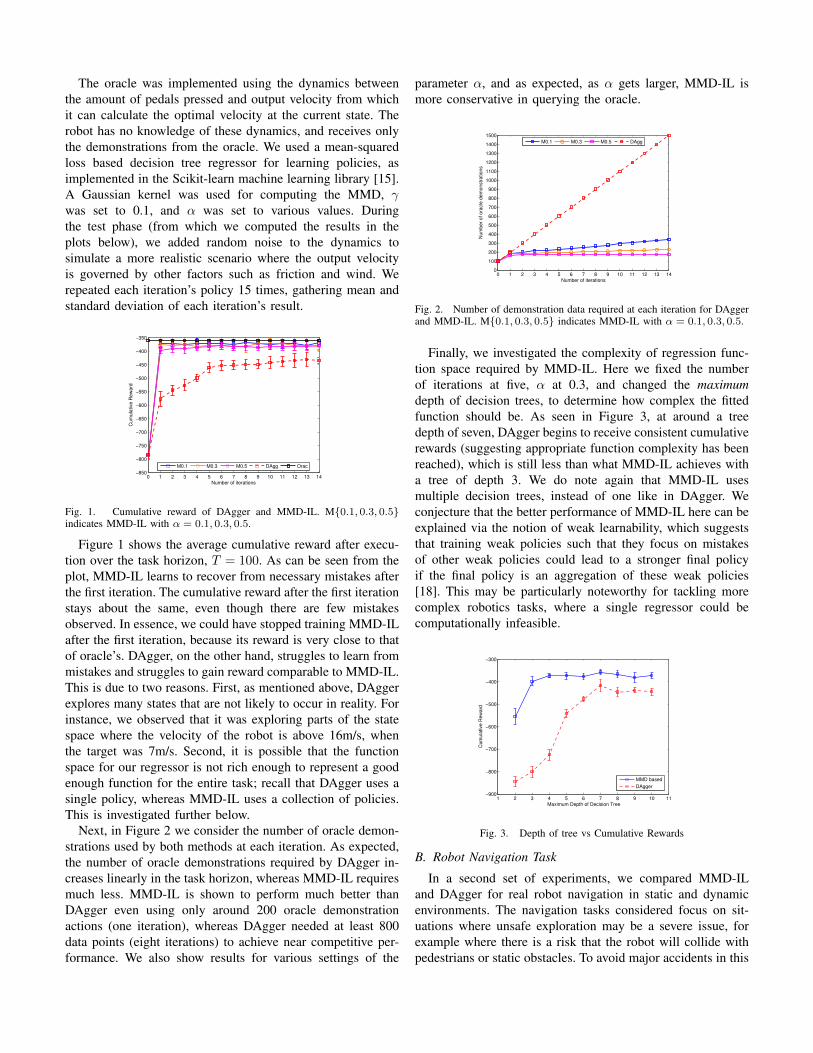
Fig. 1. Cumulative reward of DAgger and MMD-IL. M{0.1, 0.3, 0.5}indicates MMD-IL with α = 0.1, 0.3, 0.5.

Figure 1 shows the average cumulative reward after execu-tion over the task horizon, T = 100. As can be seen from theplot, MMD-IL learns to recover from necessary mistakes afterthe first iteration. The cumulative reward after the first iterationstays about the same, even though there are few mistakesobserved. In essence, we could have stopped training MMD-ILafter the first iteration, because its reward is very close to thatof oracle’s. DAgger, on the other hand, struggles to learn frommistakes and struggles to gain reward comparable to MMD-IL.This is due to two reasons. First, as mentioned above, DAggerexplores many states that are not likely to occur in reality. Forinstance, we observed that it was exploring parts of the statespace where the velocity of the robot is above 16m/s, whenthe target was 7m/s. Second, it is possible that the functionspace for our regressor is not rich enough to represent a goodenough function for the entire task; recall that DAgger uses asingle policy, whereas MMD-IL uses a collection of policies.This is investigated further below.

Next, in Figure 2 we consider the number of oracle demon-strations used by both methods at each iteration. As expected,the number of oracle demonstrations required by DAgger in-creases linearly in the task horizon, whereas MMD-IL requiresmuch less. MMD-IL is shown to perform much better thanDAgger even using only around 200 oracle demonstrationactions (one iteration), whereas DAgger needed at least 800data points (eight iterations) to achieve near competitive per-formance. We also show results for various settings of the

parameter α, and as expected, as α gets larger, MMD-IL ismore conservative in querying the oracle.

0 1 2 3 4 5 6 7 8 9 10 11 12 13 140

100

200

300

400

500

600

700

800

900

1000

1100

1200

1300

1400

1500

Number of iterations

Nu

mb

er

of

ora

cle

de

mo

nstr

atio

ns

M0.1 M0.3 M0.5 DAgg

Fig. 2. Number of demonstration data required at each iteration for DAggerand MMD-IL. M{0.1, 0.3, 0.5} indicates MMD-IL with α = 0.1, 0.3, 0.5.

Finally, we investigated the complexity of regression func-tion space required by MMD-IL. Here we fixed the numberof iterations at five, α at 0.3, and changed the maximumdepth of decision trees, to determine how complex the fittedfunction should be. As seen in Figure 3, at around a treedepth of seven, DAgger begins to receive consistent cumulativerewards (suggesting appropriate function complexity has beenreached), which is still less than what MMD-IL achieves witha tree of depth 3. We do note again that MMD-IL usesmultiple decision trees, instead of one like in DAgger. Weconjecture that the better performance of MMD-IL here can beexplained via the notion of weak learnability, which suggeststhat training weak policies such that they focus on mistakesof other weak policies could lead to a stronger final policyif the final policy is an aggregation of these weak policies[18]. This may be particularly noteworthy for tackling morecomplex robotics tasks, where a single regressor could becomputationally infeasible.

1 2 3 4 5 6 7 8 9 10 11−900

−800

−700

−600

−500

−400

−300

Maximum Depth of Decision Tree

Cu

mu

lative

Re

wa

rd

MMD based

DAgger

Fig. 3. Depth of tree vs Cumulative Rewards

B. Robot Navigation Task

In a second set of experiments, we compared MMD-ILand DAgger for real robot navigation in static and dynamicenvironments. The navigation tasks considered focus on sit-uations where unsafe exploration may be a severe issue, forexample where there is a risk that the robot will collide withpedestrians or static obstacles. To avoid major accidents in this

early phase of development, we do restrict our experiments toa controlled laboratory environment. We begin with a first setof experiments involving only static (but unmapped) obstacles,and then move to a second set of experiments involvingdynamic obstacles, in the form of moving pedestrians. In thiscase, the robot needs to not only avoid the pedestrians, butalso maintain a socially acceptable distance, therefore the useof imitation learning is particularly appropriate since notionssuch as socially acceptable movement are difficult to defineusing a standard cost function.

The robot used for these experiments is a robotic wheelchairequipped with an RGB-D (Kinect) sensor [6], as shown inFigure 4. Unlike the previous set of experiments, the state ofthe system here is not known precisely, and must be inferredin real-time from the sensor data. The camera provides apoint cloud containing 3D coordinates of the surroundingobstacles, as well as RGB information for each point in thecloud. For the static environment experiment, we set up a

Fig. 4. Picture of the robotic wheelchair equipped with Kinect

track that is approximately 3m wide and 15m long, in whichthree static obstacles were placed. The distance from the goaland the initial position of the robot was approximately 13m.While getting to the goal, the robot had to avoid all threeobstacles and stay inside the track. The dynamic environmentexperiment was also conducted in the same track, but theenvironment involved a static obstacle and a pedestrian thatis trying to reach the robot’s initial position from robot’s goal(i.e. they need to exchange positions in a narrow hallway). Therobot therefore has to simultaneously avoid the static obstacleand the moving pedestrian, while staying inside the track andgetting to its goal.

The action space is a continuous two dimensional vectorspace representing angular and linear velocities of the robot.The state space is defined by environmental features suchas obstacle densities and velocities extracted from the pointcloud. We used 3×7 grid cells, each grid cell being 1m by1m, to represent the environmental feature information in eachcell. To compute density of a cell, we counted the numberof points in the cloud belonging to that cell. Computing thevelocity in a cell involved several steps. First, we used 2Doptical flow algorithm [12] on two consecutive RGB imagesprovided by Kinect, which gives us correspondence from eachpixel of RGB image at time t− 1 to a pixel of RGB image at

time t. The correspondence information between two frameswas then transferred to 3D space by mapping each pixel to apoint in the point cloud at t− 1 and t accordingly. Then, thevelocity of a point was calculated by simply subtracting the3D coordinate of a point in t−1 from corresponding point in t.Finally, velocity of each cell was calculated by averaging thevelocity of each point in that cell. For dynamic environmentexperiment, this gave us a 63 continuous dimensional statespace (3×7 grid cells * 3 environmental features (density, and2 horizontal velocities). For the static environment, we did notuse the velocity information (=21 dimensional state space).

To train the robot, we followed Algorithm 1 and DAgger.In the initial iteration, both MMD-IL and DAgger were givena demonstration trajectory of how to avoid static and dynamicobstacles and get to the goal by a human pilot (oracle)who tele-operated the robot. For MMD-IL, we allowed themaximum oracle monitoring (i.e. α = 0) as the collision withdynamic obstacles needed to be prevented (for the safety ofthe pedestrian). At each iteration, we executed the previousiteration’s policy while applying π∗ if it is different from therobot’s policy by γ, that we set using domain knolwedge2.As a result, the oracle was able to guide the robot when itwas about to go out of the track or collide with an obstacle.For DAgger, the policy was executed and the oracle providedactions, but did not intervene (as per the algorithm’s definition)until a collision was imminent, at which point the explorationwas manually terminated by the operator and the dataset wasaggregated.

To test each iteration’s policy πi, we stopped gathering dataand executed the policy. If the policy was going to make amistake (i.e. hit one of the obstacles or go outside of thetrack), the oracle intervened and corrected its mistake so thatthe robot could get to the goal. The purpose of the oracleintervention in the test phase was to be able to numericallycompare the policies throughout the whole task horizon T .Otherwise, as these policies have not finished training, it ishard to numerically compare their performances throughoutthe task horizon as they tend to collide with obstacles andgo out of the track. To compare two algorithms, we used theoracle intervention ratio calculated by |S

∗|T , where S∗ is the

set of states in which the oracle intervened. We repeated thenavigation task using each iteration’s policy four times, to getthe mean and standard deviation of the ratio. Note that thisratio is analogous to classification error, because S∗ is the setof mistakes of the policy and T is the total number of test set.

1) Static Environment: Figure 6 shows the trajectory resultsof MMD-IL and DAgger. We observe that MMD-IL almostnever makes the same mistake twice. For instance, in the firstiteration it made mistakes close to the goal, but in seconditeration there are no mistakes at this region. Likewise, in thesecond iteration it makes mistakes when avoiding the thirdobstacle, but in the third iteration this is prevented. In the

2The linear and angular velocities of the robot are mapped to 0 to 1.0 scale.We set γ to 0.2.

Fig. 6. Example trajectories executed by policies in iterations 1 to 4, left to right, for MMD-IL(top) and for iterations 1,3,5 and 8 DAgger (bottom). Initialhuman demonstration, D∗ (black - this is the same in all panels), each iteration’s policy (dotted blue), and oracle’s interventions during the execution of thepolicy (red). Obstacles (pink squares), and track(pink lines). The initial position of the robot is at the right and the goal position is at the left.

1 2 3 4 5 6 7 8 90

0.05

0.1

0.15

0.2

0.25

0.3

0.35

0.4

0.45

Number of iterations

Ora

cle

In

terv

en

tio

n R

atio

MMD−IL

DAgger

Fig. 5. Oracle intervention ratio during the execution of each iteration’spolicy for static environment.

final iteration, it successfully avoids all three obstacles andreaches the goal, behaving very similarly to the oracle.

In contrast, DAgger struggles to learn to recover frommistakes. For instance, in the first iteration it started makingmistakes near the second obstacle until the end. The mistakesat these regions persisted until iteration three. We would alsolike to note that for DAgger, it was harder for the oracle toprovide the optimal demonstration than MMD-IL because theoracle’s input actions were not executed. For instance, whenthe robot was getting closer to an obstacle, it was hard for theoracle to know how much to turn because the oracle controlsthe robot not only by how close the robot is to the obstacle,but also by direction and speed of the robot. Since the robotwas not executing the oracle’s actions, these factors were hardto consider and the oracle ended up giving suboptimal policy.This lead to a suboptimal final policy for DAgger as shownin the bottom right-most panel of Figure 6, which features“wiggling” motions.

Figure 5 shows how often the oracle had to intervene duringthe navigation to make the robot get to the goal. As the plotshows, MMD-IL learns to navigate by itself after iteration 3,compared to iteration 7 for DAgger. This again supports ourclaim that MMD-IL requires much less oracle demonstrations.

2) Dynamic Environment: This experiment involved apedestrian that interfered with the robot’s trajectory. Thepedestrian was asked to navigate freely to get to its goal,except to move towards the static obstacle. While the pedes-trian showed irregular trajectories, the general trajectories wereeither moving to the right to avoid the robot, or movingforward and then slightly to the right. It all depended on whomoved first; if the pedestrian moved first, it was usually the

case that the pedestrian moved to the right to avoid the robot.If the robot moved first to the right to avoid the static obstacleand pedestrian, the pedestrian simply moved forward.

In the initial oracle demonstration step, the pedestrianhappened to move forward so the oracle turned to the right inan attempt to avoid both approaching pedestrian and the staticobstacle on the left. Due to this reason, the policy learned havea tendency to move towards right first, but learns to stop thismotion and go straight if the pedestrian is moving towards theright. The final policies’ trajectories are shown in Figure 7.

Fig. 7. Left: Case where the pedestrian moved forward. Right: Case where thepedestrian moved to the right. Oracle’s initial trajectory (black), final policyof MMD-IL (dotted blue) , and final policy of DAgger (red) are shown. Thegreen arrows are the approximate pedestrian trajectories (manually annotated).

As the figure shows, MMD-IL showed a trajectory that ismuch more socially adaptive when trying to avoid the pedes-trian, by imitating the oracle almost perfectly at these situa-tions. Once both pedestrian and static obstacles are avoided, itdeviates from the oracle’s trajectory but this is unimportant asthere are no more obstacles. In contrary, DAgger’s final policyinvolved moving towards the static obstacle, and waiting untilthe pedestrian passed. This is a less efficient policy, and isa direct result of the fact that when the oracle’s policies arenot being executed, the oracle cannot keep the demonstrationswithin the distribution of the optimal policy. This policy is notonly suboptimal but also socially ineffective, in that it strayedtoo close to the pedestrian.

Figure 8 shows the oracle intervention ratio plot. Again,MMD-IL learned to navigate in this environment with lessdemonstration data than DAgger. Note that the high variancewas caused by the irregular trajectories of the pedestrian.

V. RELATED WORK

There are other supervised imitation learning algorithmswhich query the oracle incrementally, besides DAgger. In [8],

1 2 3 4 5 6 7 8 90

0.1

0.2

0.3

0.4

0.5

0.6

0.7

0.8

Number of iterations

Ora

cle

In

terv

en

tio

n R

atio

MMD−IL

DAgger

Fig. 8. Oracle intervention ratio during the execution of each iteration’spolicy for dynamic environment.

a confidence-based imitation learning is proposed. The idea isto employ a Gaussian Mixture Model per action label, and thenuse certainty of a classification output to determine when toquery the oracle. The limitation of this work is that the querymetric restricts the choice of classifier to a probabilistic one.In [9], this work was extended to use other metrics such asdistance to the closest point in a training dataset and distanceto the decision boundary. Another line of work is feedbackbased imitation learning, in which the agent receives feedbackfrom the oracle as to correct the behaviour of the current policy[3, 5]. The idea is to use an Markov Decision Process, in whichrewards are specified by the oracle feedback, and to correctthe current policy such that it maximizes the return. Ourintuition behind MMD-IL is that these additional queries andfeedbacks are required because state distribution is differentwhen policy changes. The key difference between MMD-ILand these works is that it queries the oracle only when there isa significant discrepancy in state distributions, as measured viaMMD, and corrects the policy only when the current policymakes a mistake. Moreover, MMD-IL provides theoreticalguarantee using the reduction from imitation learning to no-regret online learning.

VI. CONCLUSION

In this work we proposed MMD-IL, an imitation learningalgorithm that is more data efficient and safer to use in practicethan the state-of-art imitation learning method DAgger, albeitat the cost of some extra computation. We also showed thatMMD-IL guarantees a loss linear in terms of the task horizon,as in standard supervised learning tasks. Moreover, MMD-ILcomes with pre-defined parameters, through which the usercan control how much demonstration data is collected, andwhen the oracle’s policy should be used. MMD-IL showedgood empirical performance in a variety of tasks, includingnavigating in the presence of unmodeled static and dynamicobstacles using standard sensing technology. MMD-IL out-performed DAgger in all tasks considered, mainly due to itsability to learn to quickly recover from mistakes by using theoracle to guide the learning, though limiting interventions tokey areas by using the MMD criterion. The improvement inperformance, however, was achieved at a extra computationalcost of O(m). In future, we hope to integrate imitation learningwith learning by trial-and-error, or reinforcement learning, as

to consider the case where we only have small number oforacle data, or when the oracle is sub-optimal.

ACKNOWLEDGEMENT

Authors would like to thank Stephane Ross and Doina Precupfor helpful discussions. Many thanks to A. Sutcliffe, A. el Fathi,H. Nguyen and R. Gourdeau for their contributions to the empiricalevaluation. Funding was provided by NSERC (NCNFR), FQRNT(INTER and REPARTI) and CIHR (CanWheel)

REFERENCES

[1] P. Abbeel, A. Coates, M. Quigley, and A. Y. Ng. An applicationof reinforcement learning to aerobatic helicopter flight. In NIPS19, 2007.

[2] P. Abbeel, D. Dolgov, A. Y. Ng, and S. Thrun. Apprenticeshiplearning for motion planning, with application to parking lotnavigation. In IROS, 2008.

[3] B.D. Argall, B. Browning, and M. Veloso. Learning bydemonstration with critique from a human teacher. 2009.

[4] B.D. Argall, S. Chernova, M. Veloso, and B. Browning. Asurvey of robot learning from demonstration. Robotics andAutonomous Systems, 57, 2009.

[5] B.D. Argall, B. Browning, and M. Veloso. Policy feedbackfor refinement of learned motion control on a mobile robot.International Journal of Social Robotics, 4, 2012.

[6] A. Atrash, R. Kaplow, J. Villemure, R. West, H. Yamani, andJ. Pineau. Development and validation of a robust speechinterface for improved human-robot interaction. InternationalJournal of Social Robotics, 1, 2009.

[7] J. Berg, S. Miller, D. Duckworth, H. Hu, A. Wan, X. Fu,K. Goldberg, and P. Abbeel. Superhuman performance ofsurgical tasks by robots using iterative learning from human-guided demonstrations. In ICRA, 2010.

[8] S. Chernova and M. Veloso. Confidence-based policy learningfrom demonstration using gaussian mixture models. In AAMAS,2007.

[9] S. Chernova and M. Veloso. Interactive policy learning throughconfidence-based autonomy. Journal of Artificial IntelligenceResearch, 34, 2009.

[10] A. Gretton, K. Borgwardt, M. Rasch, B. Schlkopf, andA. Smola. A kernel method for the two sample problem. InNIPS, 2007.

[11] T. Hester, M. Quinlan, and P. Stone. RTMBA: A real-timemodel-based reinforcement learning architecture for robot con-trol. In ICRA, 2012.

[12] B. Horn and B. Schunck. Determining optical flow. Artif. Intell.,17, 1981.

[13] S. M. Kakade and S. Shalev-shwartz. Mind the duality gap:Logarithmic regret algorithms for online optimization. In NIPS,2008.

[14] Y. LeCun, U. Muller, J. Ben, E. Cosatto, and B. Flepp. Off-roadobstacle avoidance through end-to-end learning. In NIPS, 2005.

[15] F. Pedregosa, G. Varoquaux, A. Gramfort, V. Michel, B. Thirion,O. Grisel, M. Blondel, P. Prettenhofer, R. Weiss, V. Dubourg,J. Vanderplas, A. Passos, D. Cournapeau, M. Brucher, M. Perrot,and E. Duchesnay. Scikit-learn: Machine learning in Python.Journal of Machine Learning Research, 12, 2011.

[16] S. Ross and J. A. Bagnell. Efficient reductions for imitationlearning. In AISTATS, 2010.

[17] S. Ross, G. Gordon, and J. A. Bagnell. A reduction of imitationlearning and structured prediction to no-regret online learning.In AISTATS, 2011.

[18] R. Schapire. The strength of weak learnability. MachineLearning, 5, 1990.