Maximum Likelihood Estimation in Latent Class Models for

Maximum Likelihood Estimation in Latent Class

Models for Contingency Table Data

Stephen E. FienbergDepartment of Statistics, MachineLearning Department and Cylab

Carnegie Mellon UniversityPittsburgh, PA 15213-3890 USA

Patricia HershDepartment of Mathematics

Indiana UniversityBloomington, IN 47405-7000 USA

Alessandro RinaldoDepartment of Statistics


Yi ZhouMachine Learning Department


i

ii

Abstract

Statistical models with latent structure have a history going back tothe 1950s and have seen widespread use in the social sciences and, more re-cently, in computational biology and in machine learning. Here we studythe basic latent class model proposed originally by the sociologist PaulF. Lazarfeld for categorical variables, and we explain its geometric struc-ture. We draw parallels between the statistical and geometric propertiesof latent class models and we illustrate geometrically the causes of manyproblems associated with maximum likelihood estimation and related sta-tistical inference. In particular, we focus on issues of non-identifiabilityand determination of the model dimension, of maximization of the like-lihood function and on the effect of symmetric data. We illustrate thesephenomena with a variety of synthetic and real-life tables, of different di-mensions and complexities. Much of the motivation for this work stemsfrom the “100 Swiss Franks” problem, which we introduce and describein detail.

Keywords: latent class model, algebraic geometry, variety, Segre vari-ety, secant variety, effective dimension.

CONTENTS iii

Contents

1 Introduction 1

2 Latent Class Models for Contingency Tables 2

3 Geometric Description of Latent Class Models 4

4 Examples Involving Synthetic Data 84.1 Effective Dimension and Polynomials . . . . . . . . . . . . . . . . 84.2 The 100 Swiss Franks Problem . . . . . . . . . . . . . . . . . . . 10

4.2.1 Introduction . . . . . . . . . . . . . . . . . . . . . . . . . 104.2.2 Global and Local Maxima . . . . . . . . . . . . . . . . . . 124.2.3 Unidentifiable Space . . . . . . . . . . . . . . . . . . . . . 134.2.4 Plotting the Log-likelihood Function . . . . . . . . . . . . 164.2.5 Further Remarks and Open Problem . . . . . . . . . . . . 16

5 Two Applications 265.1 Example: Michigan Influenza . . . . . . . . . . . . . . . . . . . . 265.2 Data From the National Long Term Care Survey . . . . . . . . . 27

6 On Symmetric Tables and the MLE 296.1 Introduction and Motivation . . . . . . . . . . . . . . . . . . . . . 316.2 Preservation of Marginals and Some Consequences . . . . . . . . 346.3 The 100 Swiss Franks Problem . . . . . . . . . . . . . . . . . . . 37

7 Conclusions 39

8 Acknowledgments 39

A Algebraic Geometry 40A.1 Polynomial Ring, Ideal and Variety . . . . . . . . . . . . . . . . . 40A.2 Segre Variety and Secant Variety . . . . . . . . . . . . . . . . . . 44

B Symbolic Software of Computational Algebra 47B.1 Computing the dimension of the image variety . . . . . . . . . . 47B.2 Solving Polynomial Equations . . . . . . . . . . . . . . . . . . . . 49B.3 Plotting Unidentifiable Space . . . . . . . . . . . . . . . . . . . . 52B.4 Surf Script . . . . . . . . . . . . . . . . . . . . . . . . . . . . . . 53

C Proof of the Fixed Points for 100 Swiss Franks Problem 55

D Matlab Codes 57

1 INTRODUCTION 1

1 Introduction

Latent class (LC) or latent structure analysis models were introduced in the1950s in the social science literature to model the distribution of dichotomousattributes based on a survey sample from a population of individuals organizedinto distinct homogeneous classes according to an unobservable attitudinal fea-ture. See Anderson (1954), Gibson (1955), Madansky (1960) and, in particular,Henry and Lazarfeld (1968). These models were later generalized in Goodman(1974), Haberman (1974), Clogg and Goodman (1984) as models for the jointmarginal distribution of a set of manifest categorical variables, assumed to beconditionally independent given an unobservable or latent categorical variable,building upon the then recently developed literature on log-linear models forcontingency tables. More recently, latent class models have been described andstudied as special cases of a larger class of directed acyclic graphical modelswith hidden nodes, sometimes referred to as Bayes nets, Bayesian networks, orcausal models, e.g., see Lauritzen (1996), Cowell et al. (1999), Humphreys andTitterington (2003) and, in particular, Geiger et al. (2001). A number of recentpapers have established fundamental connections between the statistical prop-erties of latent class models and their algebraic and geometric features, e.g., seeSettimi and Smith (1998, 2005), Smith and Croft (2003), Rusakov and Geiger(2005),Watanabe (2001) and Garcia et al. (2005).

Despite these recent important theoretical advances, the fundamental statis-tical tasks of estimation, hypothesis testing and model selection remain surpris-ingly difficult and, in some cases, infeasible, even for small latent class models.Nonetheless, LC models are widely used and there is a “folklore” associatedwith estimation in various computer packages implementing algorithms such asEM for estimation purposes, e.g., see Uebersax (2006a,b).

The goal of this article is two-fold. First, we offer a simplified geometricand algebraic description of LC models and draw parallels between their sta-tistical and geometric properties. The geometric framework enjoys notable ad-vantages over the traditional statistical representation and, in particular, offersnatural ways of representing singularities and non-identifiability problems. Fur-thermore, we argue that the many statistical issues encountered in fitting andinterpreting LC models are a reflection of complex geometric attributes of theassociated set of probability distributions. Second, we illustrate with examples,most of which quite small and seemingly trivial, some of the computational,statistical and geometric challenges that LC models pose. In particular, we fo-cus on issues of non-identifiability and determination of the model dimension, ofmaximization of the likelihood function and on the effect of symmetric data. Wealso show how to use symbolic software from computational algebra to obtain amore convenient and simpler parametrization and for unravelling the geometricfeatures of LC models. These strategies and methods should carry over to morecomplex latent structure models, such as in Bandeen-Roche et al. (1997).

In the next section, we describe the basic latent class model and its statisticalproperties and, in Section 3, we discuss the geometry of the models. In Section 4,we turn to our examples exemplifying the identifiability issue and the complexity

2 LATENT CLASS MODELS FOR CONTINGENCY TABLES 2

of the likelihood function, with a novel focus on the problems arising fromsymmetries in the data. Finally, we present some computational results for tworeal-life examples, of small and very large dimension.

2 Latent Class Models for Contingency Tables

Consider k categorical variables, X1, . . . , Xk, where each Xi takes value on thefinite set [di] ≡ {1, . . . , di}. Letting D =

⊗ki=1[di], RD is the vector space of

k-dimensional arrays of the format d1 × . . . × dk, with a total of d =∏

i di

entries. The cross-classification of N independent and identically distributedrealizations of (X1, . . . , Xk) produces a random integer-valued vector n ∈ RD,whose coordinate entry nii,...,ik

corresponds to the number of times the labelcombination (i1, . . . , ik) was observed in the sample, for each (i1, . . . , ik) ∈ D.The table n has a Multinomial(N,p) distribution, where p is a point in the(d− 1)-dimensional probability simplex ∆d−1 with coordinates

pi1,...,ik= Pr {(X1, . . . , Xk) = (i1, . . . , ik)} , (i1, . . . , ik) ∈ D.

Let H be an unobservable latent variable, defined on the set [r] = {1, . . . , r}.In its most basic version, also known as the naive Bayes model, the LC modelpostulates that, conditional on H, the variables X1, . . . , Xk are mutually in-dependent. Specifically, the joint distributions of X1, . . . , Xk and H form thesubset V of the probability simplex ∆dr−1 consisting of points with coordinates

pi1,...,ik,h = p(h)1 (i1) . . . p

(h)k (ik)λh, (i1, . . . , ik, h) ∈ D × [r], (1)

where λh is the marginal probability Pr{H = h} and p(h)l (il) is the condi-

tional marginal probability Pr{Xl = il|H = h}, which we assume to be strictlypositive for each h ∈ [r] and (i1, . . . , ik) ∈ D.

The log-linear model specified by the polynomial mappings (1) is a decom-posable graphical model (see, e.g, Lauritzen, 1996) and V is the image set of ahomeomorphism from the parameter space

Θ ≡{

θ: θ = (p(h)1 (i1) . . . p

(h)k (ik), λh), (i1, . . . , ik, h) ∈ D × [r]

}=

⊗i ∆di−1 ×∆r−1,

so that global identifiability is guaranteed. The remarkable statistical propertiesof this type of models and the geometric features of the set V are well understood.Statistically, equation (1) defines a linear exponential family of distributions,though not in its natural parametrization. The maximum likelihood estimates,or MLEs, of λh and p

(h)l (il) exist if and only if the minimal sufficient statistics,

i.e., the empirical joint distributions of (Xi,H) for i = 1, 2, . . . , k, are strictlypositive and are given in closed form as rational functions of the observed two-way marginal distributions between Xi and H for i = 1, 2, . . . , k. The log-likelihood function is strictly concave and the maximum is always attainable,

2 LATENT CLASS MODELS FOR CONTINGENCY TABLES 3

possibly on the boundary of the parameter space. Furthermore, the asymptotictheory of goodness-of-fit testing is fully developed.

Geometrically, we can obtain the set V as the intersection of ∆dr−1 withan affine variety (see, e.g., Cox et al., 1996) consisting of the solutions set of asystem of r

∏i

(di

2

)homogeneous square-free polynomials. For example, when

k = 2, each of these polynomials take the form of quadric equations of the type

pi1,i2,hpi′1,i′2,h = pi′1,i2,hpi1,i′2,h, (2)

with i1 6= i′1, i2 6= i′2 and for each fixed h. Provided the probabilities are strictlypositive, equations of the form (2) specify conditional odds ratio of 1, for everypair (Xi, Xi′) given H = h. Furthermore, for each given h, the coordinateprojections of the first two coordinates of the points satisfying (2) trace thesurface of independence inside the simplex ∆d−1. The strictly positive points ofV form a smooth manifold whose dimension is r

∏i(di−1)+(r−1) and whose co-

dimension corresponds to the number of degrees of freedom. The singular pointsof V all lie on the boundary of the simplex ∆dr−1 and identify distributions withdegenerate probabilities along some coordinates. More generally, the singularlocus of V can be described similarly in terms of stratified components of V,whose dimensions and co-dimensions can also be computed explicitly.

Under the LC model, the variable H is unobservable and the new model H isa r-class mixture over the exponential family of distributions prescribing mutualindependence among the manifest variables X1, . . . , Xk. Geometrically, H is theset of probability vectors in ∆d−1 obtained as the image of the marginalizationmap from ∆dr−1 onto ∆d−1 which consists of taking the sum over the coordinatecorresponding to the latent variable. Formally, H is made up of all probabilityvectors in ∆d−1 with coordinates satisfying the accounting equations (see, e.g.,Henry and Lazarfeld, 1968)

pi1,...,ik=

∑h∈[r]

pi1,...,ik,h =∑h∈[r]

p(h)1 (i1) . . . p

(h)k (ik)λh, (3)

where (i1, . . . , ik, h) ∈ D × [r].Despite being expressible as a convex combination of very well-behaved mod-

els, even the simplest form of the LC model (3) is far from being well-behavedand, in fact, shares virtually none of the properties of the standard log-linearmodels. In particular, the latent class models specified by equations (3) donot define exponential families, but instead belong to a broader class of modelscalled stratified exponential families (see Geiger et al., 2001), whose propertiesare much weaker and less well understood. The minimal sufficient statisticsfor an observed table n are the observed counts themselves and we can achieveno data reduction via sufficiency. The model may not be identifiable, becausefor a given p ∈ ∆d−1 satisfying (3), there may be a subset of Θ, known asthe non-identifiable space, consisting of parameter points all satisfying the sameaccounting equations. The non-identifiability issue has in turn considerablerepercussions on the determination of the correct number of degrees of freedomfor assessing model fit and, more importantly, on the asymptotic properties

3 GEOMETRIC DESCRIPTION OF LATENT CLASS MODELS 4

of standard model selection criteria (e.g. likelihood ratio statistic and othergoodness-of-fit criteria such as BIC, AIC, etc), whose applicability and correct-ness may no longer hold.

Computationally, maximizing the log-likelihood can be a rather laboriousand difficult task, particularly for high dimensional tables, due to lack of con-cavity, the presence of local maxima and saddle points, and singularities in theobserved Fisher information matrix. Geometrically, H is no longer a smoothmanifold in the relative interior of ∆d−1, with singularities even at probabilityvectors with strictly positive coordinates, as we show in the next section. Theproblem of characterizing the singular locus of H and of computing the dimen-sions of its stratified components (and of the tangent spaces and tangent conesof its singular points) is of statistical importance: singularity points of H areprobability distributions of lower complexity, in the sense that they are speci-fied by lower-dimensional subsets of Θ, or, loosely speaking, by less parameters.Because the sample space is discrete, although the singular locus of H has typ-ically Lebesgue measure zero, there is nonetheless a positive probability thatthe maximum likelihood estimates end up being either a singular point in therelative interior of the simplex ∆d−1 or a point on the boundary. In both cases,standard asymptotics for hypothesis testing and model selection fall short.

3 Geometric Description of Latent Class Models

In this section, we give a geometric representation of latent class models, sum-marize existing results and point to some of the relevant mathematical literature.For more details, see Garcia et al. (2005) and Garcia (2004).

The latent class model defined by (3) can be described as the set of allconvex combinations of r-tuple of points lying on the surface of independenceinside ∆d−1. Formally, let

σ: ∆d1−1 × . . .×∆dk−1 → ∆d−1

(p1(i1), . . . , pk(ik)) 7→∏

j pj(ij)

be the map that sends the vectors of marginal probabilities into the k-dimensionalarray of joint probabilities for the model of complete independence. The setS ≡ σ(∆d1−1 × . . . × ∆dk−1) is a manifold in ∆d−1 known in statistics as thesurface of independence and in algebraic geometry (see, e.g. Harris, 1992) as(the intersection of ∆d−1 with) the Segre embedding of Pd1−1 × . . . × Pdk−1

into Pd−1. The dimension of S is∏

i(di − 1), i.e., the dimension of the corre-sponding decomposable model of mutual independence. The set H can then beconstructed geometrically as follows. Pick any combination of r points alongthe hyper-surface S, say p(1), . . . ,p(r), and determine their convex hull, i.e. theconvex set consisting of all points of the form

∑h p(h)λh, for some choice of

(λ1, . . . , λr) ∈ ∆r−1. The coordinates of any point in this new subset satisfy,by construction, the accounting equations (3). In fact, the closure of the unionof all such convex hulls is precisely the latent class model H. In algebraic ge-ometry, H would be described as the intersection of ∆d−1 with the r-th secant


variety of the Segre embedding mentioned above. More about the Segre andsecant varieties can be found in the appendix A.2.

Figure 1: Surface of independence for the 2× 2 table with 3 secant lines.

Example 3.1 The simplest example of a latent class model is for a 2× 2 tablewith one latent variable with r = 2. The surface of independence, i.e. theintersection of the simplex ∆3 with the Segre variety, is shown in Figure 1. Thesecant variety for this latent class models is the union of all the secant lines, i.e.the lines connecting any two distinct points lying on the surface of independence.Figure 1 displays three such secant lines. It is not too hard to picture that theunion of all such secant lines is the enveloping simplex ∆3 and, therefore, Hfills up all the available space (for formal arguments, see Catalisano et al., 2002,Proposition 2.3).

The model H is not a smooth manifold. Instead, it is a semi-algebraic set(see, e.g., Benedetti, 1990), clearly singular on the boundary of the simplex,but also at strictly positive points along the (r − 1)st secant variety, (both ofLebesgue measure zero). This means that the model is singular at all points inH which satisfy the accounting equations with one or more of the λh’s equalto zero. In Example 3.1 above, the surface of independence is a singular locusfor the latent class model. From the statistical viewpoint, singular points of Hcorrespond to simpler models for which the number of latent classes is less thanr (possibly 0). As usual, for these points one needs to adjust the number ofdegrees of freedom to account for the larger tangent space.

Unfortunately, we have no general closed-form expression for computing thedimension of H and the existing results only deal with specific cases. Simple


considerations allow us to compute an upper bound for the dimension of H, asfollows. As Example 3.1 shows, there may be instances for which H fills up theentire simplex ∆d−1, so that d− 1 is an attainable upper bound. Counting thenumber of free parameters in (3), we can see that this dimension cannot exceedr∑

i(di − 1) + r − 1, (c.f. Goodman, 1974, page 219). This number, the stan-dard dimension, is the dimension of the fully observable model of conditionalindependence. Incidentally, this value can be determined mirroring the geomet-ric construction of H as follows (c.f. Garcia, 2004). The number r

∑i(di − 1)

arises from the choice of r points along the∑

i(di − 1)-dimensional surface ofindependence, while the term r − 1 accounts for the number of free parametersfor a generic choice of (λ1, . . . , λr) ∈ ∆r−1. Therefore, we conclude that thedimension of H is bounded by

min

{d− 1, r

∑i

(di − 1) + r − 1

}, (4)

a value known in algebraic geometry as the expected dimension of the varietyH.

Cases of latent class models with dimension strictly smaller than the ex-pected dimension have been known for a long time, however. In the statisticalliterature, Goodman (1974) noticed that the latent class models for 4 binaryobservable variables and a 3-level latent variable, whose expected dimension is14, has dimension 13. In algebraic geometry, secant varieties with dimensionsmaller than the expected dimension (4) are called deficient (e.g., see Harris,1992). In particular, Exercise 11.26 in Harris (1992) gives an example of a defi-cient secant variety, which corresponds to a latent class model for a 2-way tablewith a binary latent variable. In this case, the deficiency is 2, as is demonstratedbelow in equation (5). The true or effective dimension of a latent class model,i.e. the dimension of the semi-algeraic set H representing it, is crucial for es-tablishing identifiability and for computing correctly the number of degrees offreedom. In fact, if a model is deficient, then the pre-image of each probabilityarray in H arising from the accounting equations is a subset (in fact, a variety)of Θ called the non-dentifiable subspace, with dimension exactly equal to thedeficiency itself. Therefore, a deficient model is non-identifiable, with adjusteddegrees of freedom equal to number of degrees of freedom for the observablegraphical model plus the value of the deficiency.

The effective dimension of H is equal to the maximal rank of the Jacobianmatrix for the polynomial mapping from Θ into H given coordinatewise by(3). Geiger et al. (2001) showed that this value is equal to the dimension of Halmost everywhere with respect to the Lebsegue measure, provided the Jacobianis evaluated at strictly positive parameter points θ, and used this result to devisea simple and efficient algorithm to compute numerically the effective dimension.We include the Matlab codes for computing the numberical rank of the Jacobianin the appendix D.

Recently, in the algebraic-geometry literature, Catalisano et al. (2002, 2003)have obtained explicit formulas for the effective dimensions of some secant va-


rieties which are of statistical interest. In particular, they show that for k = 3and r ≤ min{d1, d2, d3}, the latent class model has the expected dimension andis identifiable. On the other hand, assuming d1 ≤ d2 ≤ . . . ≤ dk, H is deficientwhen

∏k−1i=1 di −

∑k−1i=1 (di − 1) ≤ r ≤ min

{dk,

∏k−1i=1 di − 1

}. Finally, under

the same conditions, H is identifiable when 12

∑i(di − 1) + 1 ≥ max{dk, r}. In

general, obtaining bounds and results of this type is highly non-trivial and isan open area of research. Refer to the appendix A.2 to see more results on theeffective dimension of secant varieties.

In the remainder of the paper, we will focus on simpler latent class modelsfor tables of dimension k = 2 and illustrate with examples the results mentionedabove. For latent class models on two-way tables, there is an alternative, quiteconvenient way of describing H by representing each p in ∆d−1 as a d1 × d2

matrix and by representing the map σ as a vector product. In fact, each point pin S is a rank one matrix obtained as p1p>2 , where p1 ∈ ∆d1−1 and p2 ∈ ∆d1−2

are the appropriate marginal distributions of X1 and X2. Then, the accountingequations for a latent class models with r-level become

p =∑

h

p(h)1 (p(h)

2 )>λh, (p1,p2, (λ1, . . . , λr)) ∈ ∆d1−1 ×∆d2−1 ×∆r−1

i.e. the matrix p is a convex combination of r rank 1 matrices lying on thesurface of independence. Therefore all points in H are non-negative matriceswith entries summing to one and with rank at most r. This simple observationallows one to compute the effective dimension of H for 2-way table as follows.In general, a real valued d1 × d2 matrix has rank r or less if and only if thehomogeneous polynomial equations corresponding to all of its (r + 1)× (r + 1)minors all vanish. Provided k < min{d1, d2}, on Rd1 × Rd2 , the zero locus ofall such equations form a determinantal variety of co-dimension (d1− r)(d2− r)(c.f. Harris, 1992, Proposition 12.2) and hence has dimension r(d1 + d2) − r2.Subtracting this value from the expected dimension (4), and taking into accountthe fact that all the points lie inside the simplex, we obtain

r(d1 + d2 − 2) + r − 1−(r(d1 + d2)− r2 − 1

)= r(r − 1). (5)

This number is also the difference between the dimension of the (fully identifi-able, i.e. of expected dimension) graphical model of conditional independenceX1 and X2 given H, and the deficient dimension of the latent class model ob-tained by marginalizing over the variable H.

The study of higher dimensional tables is still an open area of research. Themathematical machinery required to handle larger dimensions is considerablymore complicated and relies on the notions higher-dimensional tensors, ranktensors and non-negative rank tensors, for which only partial results exist. SeeKruskal (1975), Cohen and Rothblum (1993) and Strassen (1983) for details.Alternatively, Mond et al. (2003) conduct an algebraic-topological investigationof the topological properties of stochastic factorization of stochastic matricesrepresenting models of conditional independence with one hidden variable and

4 EXAMPLES INVOLVING SYNTHETIC DATA 8

Allman and Rhodes (2006, 2007) explore an overlapping set of problems framedin the context of trees with latent nodes and branches.

The specific case of k-way tables with 2 level latent variables is a fortunateexception, for which the results for 2-way tables just described apply. In fact,Landsberg and Manivel (2004) show that that these models are the same asthe corresponding model for any two-dimensional table obtained by any “flat-tening” of the d1 × . . . × dk-dimensional array of probabilities p into a two-dimensional matrix. Flattening simply means collapsing the k variables intotwo new variables with f1 and f2 levels, and re-organizing the entries of thek-dimensional tensor p ∈ ∆d−1 into a f1 × f1 matrix accordingly, where, neces-sarily, f1 + f2 =

∑i di. Then, H is the determinantal variety which is the zero

set of all 3× 3 sub-determinants of the matrix obtained by any such flattening.The second example in Section 4.1 below illustrates this result.

4 Examples Involving Synthetic Data

We further elucidate the non-identifiability phenomenon from the algebraic andgeometric point of view, and the multi-modality of the log-likelihood functionissue using small synthetic examples. In particular, in the “100 Swiss Franks”problem below, we embark on an exhaustive study of a table with symmetricdata and describe the effects of such symmetries on both the parameter spaceand the log-likelihood function. Although those examples treat simplest casesof LC models, they already exhibit considerable statistical and geometric com-plexity.

4.1 Effective Dimension and Polynomials

We show how it is possible to take advantage of the polynomial nature of equa-tions (3) to gain further insights into the algebraic properties of distributionsobeying latent class models. All the computations that follow were made inSINGULAR (Greuel et al., 2005) and are described in details, along with moreexamples, in Zhou (2007). Although in principle symbolic algebraic softwareallows one to compute the set of polynomial equations that fully characterizeLC models and their properties, this is still a rather difficult and costly taskthat can be accomplished only for smaller models.

The accounting equations (3) determine a polynomial mapping f : Θ → ∆d−1

given by(p1(i1) . . . pk(ik), λh) 7→

∑h∈[r]

p1(i1) . . . pk(ik)λh, (6)

so that the latent class model is analytically defined as its image, i.e. H = f(Θ).Then, following the geometry-algebra dictionary principle (see, e.g., Cox et al.,1996), the problem of computing the effective dimension of H can in turn begeometrically cast as a problem of computing the dimension of the image ofa polynomial map. We illustrate how this representation offers considerableadvantages with some small examples.


Consider a 2 × 2 × 2 table with r = 2 latent classes. From Proposition 2.3in Catalisano et al. (2002), the latent class models with 2 classes and 3 man-ifest variables are identifiable. The standard dimension, i.e. the dimension ofthe parameter space Θ is r

∑i(di − 1) + r − 1 = 7, which coincides with the

dimension of the enveloping simplex ∆7. Although this condition implies thatthe number of parameters to estimate is no larger than the number of cells inthe table, a case which, if violated, would entail non-identifiability, it does notguarantee that the effective dimension is also 7. This can be verified by check-ing that the symbolic rank of the Jacobian matrix of the map (6) is indeed 7,almost everywhere with respect to the Lebesgue measure. Alternatively, onecan determine the dimension of the non-identifiable subspace using computa-tional symbolic algebra. First, we consider the ideal of polynomials generatedby the 8 equations in (6) in the polynomial ring in which the (redundant) 16indeterminates are the 8 joint probabilities in ∆7 and the 3 pairs of marginalprobabilities in ∆1 for the observable variables, and the marginal probabilitiesin ∆1 for the latent variable. Then we use implicization (see, e.g., Cox et al.,1996, Chapter 3) to eliminate all the marginal probabilities and to study theGroebner basis of the resulting ideal in which the indeterminates are the jointprobabilities only. There is only one element in the basis,

p111 + p112 + p121 + p122 + p211 + p212 + p221 + p222 = 1,

which gives the trivial condition for probability vectors. This implies the map(6) is surjective, so that H = ∆7 and the effective dimension is also 7, showingidentifiability, at least for positive distributions.

Next, we consider the 2 × 2 × 3 table with r = 2. For this model, Θ hasdimension 9 and the symbolic rank of the associated Jacobian matrix is 9 aswell, so that the model is identifiable. Alternatively, using the same route asin the previous example, we see that, in this case, the image of the polynomialmapping (6) is the variety associated to the ideal whose Groebner basis consistsof the trivial equation

p111 +p112 +p113 +p121 +p122 +p123 +p211 +p212 +p213 +p221 +p222 +p223 = 1,


and four polynomials corresponding to the determinants∣∣∣∣∣∣p121 p211 p221

p122 p212 p222

p123 p213 p223

∣∣∣∣∣∣∣∣∣∣∣∣p1+1 p211 p221

p1+2 p212 p222

p1+3 p213 p223

∣∣∣∣∣∣∣∣∣∣∣∣p+11 p121 p221

p+12 p122 p222

p+13 p123 p223

∣∣∣∣∣∣∣∣∣∣∣∣p111 p121 + p211 p221

p112 p122 + p212 p222

p113 p123 + p213 p223

∣∣∣∣∣∣

(7)

where the subscript symbol “+” indicates summation over that coordinate. Thesingular codes for computing the Groebner basis are in the appendix B.1.The zero set of the above determinants coincide with the determinantal varietyspecified by the zero set of all 3× 3 minors of the 3×4 matrix p111 p121 p211 p221

p112 p122 p212 p222

p113 p123 p213 p223

(8)

which is a flattening of the 2× 2× 3 array of probabilities describing the jointdistribution for the latent class model under study. This is in accordance withthe result in Landsberg and Manivel (2004) mentioned above. Now, the deter-minantal variety given by the vanishing locus of all the 3×3 minors of the matrix(8) is the latent class model for a 3 × 4 table with 2 latent classes, which, ac-cording to (5), has deficiency equal to 2. The effective dimension of this varietyis 9, computed as the standard dimension, 11, minus the deficiency. Therefore,the effective dimension of the model we are interested is also 9 and we concludethat the model is identifiable.

Table 10 summarizes some of our numerical evaluations of the different no-tions of dimension for a different LC models. We computed the effective di-mensions by evaluating with MATLAB the numerical rank of the Jacobian matrix,based on the algorithm of Geiger et al. (2001) and also using SINGULAR, forwhich only computations involving small models were feasible.

4.2 The 100 Swiss Franks Problem

4.2.1 Introduction

Now we study the problem of fitting a non-identifiable 2-level latent class modelto a two-way table with symmetry counts. This problem was suggested by


Table 1: Different dimensions of some latent class models. The Complete Di-mension is the dimension d− 1 of the envoloping probability simplex ∆d−1. Seealso Table 1 in Kocka and Zhang (2002).

Effective Standard CompleteLatent Class Model Dimension Dimension Dimension Deficiency

∆d−1 r2× 2 2 3 5 3 03× 3 2 7 9 8 14× 5 3 17 23 19 2

2× 2× 2 2 7 7 7 02× 2× 2 3 7 11 7 02× 2× 2 4 7 15 7 03× 3× 3 2 13 13 26 03× 3× 3 3 20 20 26 03× 3× 3 4 25 27 26 13× 3× 3 5 26 34 26 03× 3× 3 6 26 41 26 05× 2× 2 3 17 20 19 24× 2× 2 3 14 17 15 13× 3× 2 5 17 29 17 06× 3× 2 5 34 44 35 110× 3× 2 5 54 64 59 5

2× 2× 2× 2 2 9 9 15 02× 2× 2× 2 3 13 14 15 12× 2× 2× 2 4 15 19 15 02× 2× 2× 2 5 15 24 15 02× 2× 2× 2 6 15 29 15 0

Bernd Sturmfels to the participants of his postgraduate lectures on AlgebraicStatistics held at ETH Zurich in the Summer semester of 2005 (where he offered100 Swiss Franks for a rigorous solution), and is described in detail as Example1.16 in Pachter and Sturmfels (2005). The observed table is

n =

4 2 2 22 4 2 22 2 4 22 2 2 4

(9)

and the 100 Swiss Franks problem requires proving that the three tables inTable 2 a) are global maxima for the the basic LC model with one binary latentvariable. For this model, the standard dimension of Θ = ∆3 × ∆3 × ∆1 is2(3 + 3) + 1 = 13 and, by (5), the deficiency is 2. Thus, the model is notidentifiable and the pre-image of each point p ∈ H by the map (6) is a 2-dimensional surface in Θ. To keep the notation light, we write αih for p

(h)1 (i)

and βjh for p(h)2 (j), where i, j = 1, . . . , 4 and α(h) and β(h) for the conditional


marginal distribution of X1 and X2 given H = h, respectively. The accountingequations for the points in H become

pij =∑

h∈{1,2}

λhαihβjh, i, j ∈ [4] (10)

and the log-likelihood function, ignoring an irrelevant additive constant, is

`(θ) =∑i,j

nij log

∑h∈{1,2}

λhαihβjh

, θ ∈ ∆3 ×∆3 ×∆1.

It is worth emphasizing, as we did above and as the previous display clearlyshows, that the observed counts are minimal sufficient statistics.

Alternatively, we can re-parametrize the log-likelihood function using di-rectly points in H rather than the points in the parameter space Θ. Recall fromour discussion in section 3 that, for this model, the 4× 4 array p is in H if andonly if each 3×3 minor vanishes. Then, we can write the log-likelihood functionas

`(p) =∑i,j

nij log pij , p ∈ ∆15, det(p∗ij) = 0 all i, j ∈ [4], (11)

where p∗ij is the 3× 3 sub-matrix of p obtained by erasing the ith row and thejth column.

Although the first order optimality conditions for the Lagrangian corre-sponding to the parametrization (11) are algebraically simpler and can be giventhe form of a system of a polynomial equations, in practice, the classical parametriza-tion (10) is used in both the EM and the Newton-Raphson implementations inorder to compute the maximum likelihood estimate of p. See Goodman (1979),Haberman (1988), and Redner and Walker (1984) for more details about thesenumerical procedures. Codes for solving equation 11 in singular are given inthe appendix B.2.

4.2.2 Global and Local Maxima

Using both EM and Newton-Raphson algorithm with several different startingpoints, we found 7 local maxima of the log-likelihood function, reported in Table2. The maximal value of the log-likelihood function was found experimentallyto be −20.8074 + const., where const. denotes the additive constant stemmingfrom the multinomial coefficient. The maximum is achieved by the three tablesof fitted values Table 2 a). The remaining four tables are local maxima of−20.8616+const., close in value to the actual global maximum. Using SINGULAR(see (Greuel et al., 2005)), we checked that the tables found satisfy the firstorder optimality conditions (11). After verifying numerically the second orderoptimality conditions, we conclude that those points are indeed local maxima.As noted in Pachter and Sturmfels (2005), the log-likelihood function also hasa few saddle points.


Table 2: Tables of fitted value corresponding to the 7 maxima of the likelihoodequation for the 100 Swiss Franks data shown in (9). a): global maximua (log-likelihood value −20.8079). b): local maxima (log-likelihood value −20.8616).

a)3 3 2 23 3 2 22 2 3 32 2 3 3

3 2 3 22 3 2 33 2 3 22 3 2 3

3 2 2 32 3 3 22 3 3 23 2 2 3

b)

8/3 8/3 8/3 28/3 8/3 8/3 28/3 8/3 8/3 22 2 2 4

8/3 8/3 2 8/38/3 8/3 2 8/32 2 4 2

8/3 8/3 2 8/3

8/3 2 8/3 8/32 4 2 2

8/3 2 8/3 8/38/3 2 8/3 8/3

4 2 2 22 8/3 8/3 8/32 8/3 8/3 8/32 8/3 8/3 8/3

A striking feature of the global maxima in Table 2 is their invariance underthe action of the symmetric group on four elements acting simultaneously on therow and columns. Different symmetries arise for the local maxima. We will givean explicit representation of these symmetries under the classical parametriza-tion (10) in the next section.

Despite the simplicity and low-dimensionality of the LC model for this tableand the strong symmetric features of the data, we have yet to provide a purelymathematical proof that the three top arrays in Table 2 correspond to a globalmaximum of the likelihood function. We view the difficulty and complexityof the 100 Swiss Franks problem as a consequence of the inherent difficulty ofeven small LC models and perhaps an indication that the current theory hasstill many open, unanswered problems. In Section 6, we present partial resultstowards the completion of the proof.

4.2.3 Unidentifiable Space

It follows from equation (5) that the non-identifiable subspaces are a two-dimensional subsets of Θ. We give an explicit algebraic description of this space,which we will then use to obtain interpretable plots of the profile likelihood.

Firstly, we focus on the three global maxima in Table 2 a). By the well-known properties of the EM algorithm (see, e.g., Pachter and Sturmfels, 2005,Theorem 1.15), if the vector of parameters θ is a stationary point in the maxi-mization step of the EM algorithm, then θ is a critical point and hence a good


Figure 2: The 2-dimensional surface defined by equation (13), when evaluatedover the ball in R3 of radius 3, centered at the origin. The inner box is the unitcube [0, 1]3 and its intersection with the surface corresponds to solutions pointsdefining probability distributions.

candidate for a local maximum. Using this observation, it is possible to show(see Zhou, 2007) that any point in Θ satisfying the equations

α1h = α2h, α3h = α4h h = 1, 2β1h = β2h, β3h = β4h h = 1, 2∑

h λhα1hβ1h =∑

h λhα3hβ3t = 3/40∑h λhα1hβ3h =

∑h λhα3hβ1t = 2/40

(12)

is a stationary point. Notice that the first four equations in (22) require α(h) andβ(h) to each have the first and second pairs of coordinates identical, for h = 1, 2.The equation (22) defines a 2-dimensional surface in Θ. Using SINGULAR, wecan verify that, holding, for example, α11 and β11 fixed, determines all of the


other parameters according to the equations

λ1 = 180α11β11−20α11−20∗β11+6

λ2 = 1− λ1

α21 = α11

α31 = α41 = 0.5− α11

α12 = α22 = 10β11−310(4β11−1)

α32 = α42 = 0.5− α12

β21 = β11

β31 = β41 = 0.5− β11

β12 = β22 = 10α11−310(4α11−1)

β32 = β42 = 0.5− β12.

Derivation of these equations can be found in the appendix B.3. Using the elim-ination technique (see Cox et al., 1996, Chapter 3) to remove all the variablesin the system except for λ1, we are left with one equation

80λ1α11β11 − 20λ1α11 − 20λ1β11 + 6λ1 − 1 = 0. (13)

Without the constraints for the coordinates of α11, β11 and λ1 to be probabili-ties, (13) defines a two-dimensional surface in R3, depicted in Figure 2. Noticethat the axes do not intersect this surface, so that zero is not a possible valuefor α11, β11 and λ1. Because the non-identifiable space in Θ is 2-dimensional,equation (13) actually defines a bijection between α11, β11 and λ1 and the restof the parameters. Then, the intersection of the surface (13) with the unit cube[0, 1]3, depicted as a red box in Figure 2, is the projection of the non-identifiablesubspace into the 3-dimensional unit cube where α11, β11 and λ1 live. Figure3 displays two different views of this projection. In the appendices B.3 andB.4, we show how to draw these figures using singular’s graphics engine, theprogramme SURF.

The preceding arguments hold unchanged if we replace the symmetry con-ditions in the first two lines of equation (22) with either of these other twoconditions, requiring different pairs of coordinates to be identical, namely

α1h = α3h, α2h = α4h, β1h = β3h, β2h = β4h (14)

andα1h = α4h, α2h = α3h, β1h = β4h, β2h = β3h, (15)

where h = 1, 2.The non-identifiable surfaces inside Θ corresponding each to one of the three

pairs of coordinates held fixed in equations (22), (14) and (15), produce the threedistinct tables of maximum likelihood estimates reported in Table 2 a). Figure3 shows the projection of the non-identifiable subspaces for the three MLEs inTable 2 a) into the three dimensional unit cube for λ1, α11 and β11. Althougheach of these three subspaces are disjoint subsets of Θ, their lower dimensionalprojections comes out as unique. By projecting onto the different coordinates


λ1, α11 and β21 instead, we obtain two disjoint surfaces for the first, and secondand third MLE, shown in Figure 4.

Table 3 presents some estimated parameters using the EM algorithm. Thoughthese estimates are hardly meaningful, because of the non-identifiability issue,they show the symmetry properties we pointed out above and implicit in equa-tions (22), (14) and (15), and they explain the invariance under simultane-ous permutation of the fitted tables. In fact, the number of global maximais the number of different configurations of the 4 dimensional vectors of esti-mated marginal probabilities with two identical coordinates, namely 3. Thisphenomenon, entirely due to the strong symmetry in the observed table (9), iscompletely separate from the non-identrifiability issues, but just as problematic.

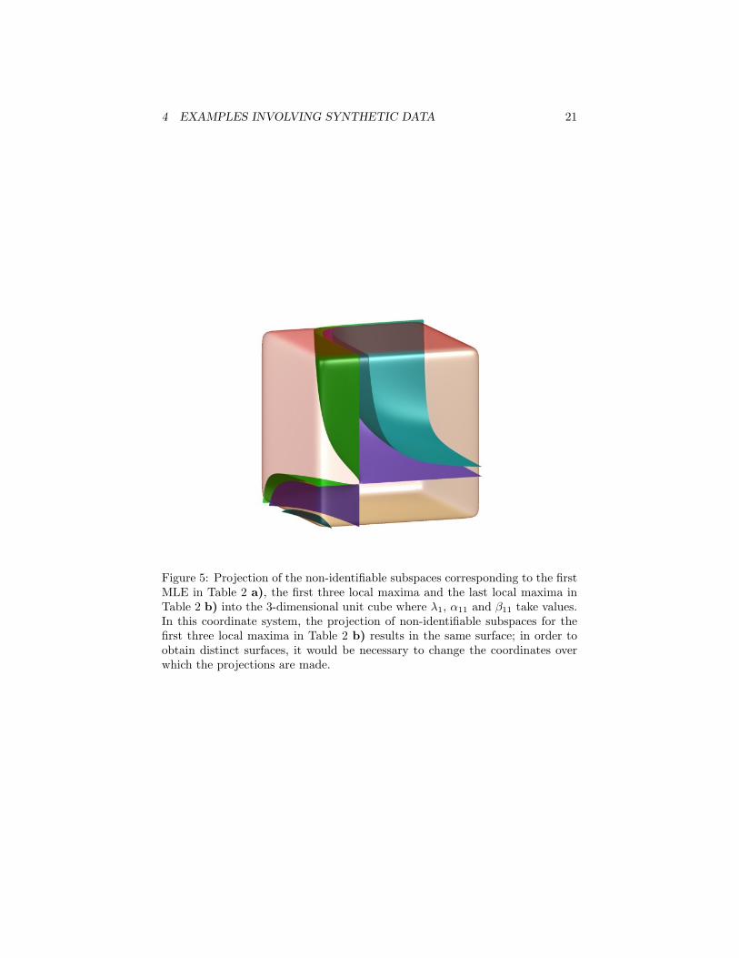
By the same token, we can show that vectors of marginal probabilities with3 identical coordinates also produce stationary points for the EM algorithms.This type of stationary points trace surfaces inside Θ which determine the localmaxima of Table 2 b). The number of these local maxima corresponds, in fact,to the number of possible configurations of 4-dimensional vectors with 3 identicalcoordinates, namely 4. Figure 5 depicts the lower dimensional projections intoλ1, α11 and β11 of the non-identifiable subspaces for the first MLE in Table 2a), the first three local maxima and the last local maxima in Table 2 b).

We can summarize our finding as follows: the maxima in Table 2 definedisjoint 2-dimensional surfaces inside the parameter space Θ, the projection ofone of them being depicted in Figure 3. While non-identifiability is a structuralfeature of these models which is independent of the observed data, the multi-plicity and invariance properties of the maximum likelihood estimates and theother local maxima is a phenomenon caused by the symmetry in the observedtable of counts.

4.2.4 Plotting the Log-likelihood Function

Having determined that the non-identifiable space is 2-dimensional and thatthere are multiple maxima, we proceed with some plots of the profile log-likelihood function. To obtain a non-trivial surface, we need to consider threeparameters. Figures 9 and 7 display the surface and contour plot respectivelyof the profile log-likelihhod function for α11 and α21 when α31 is one of thefixed parameters. Both Figures show clearly the different maxima, each lyingon the top of “ridges” of the log-likelihood surface which are placed symmet-rically with respect to each others. The position and shapes of these ridgesreflect, once again, the symmetric properties of the estimated probabilities andparameters.

4.2.5 Further Remarks and Open Problem

We conclude this section with some observations and pointers to open problems.One of the interesting aspects we came across while fitting the table (9) was

the proximity of the values of the local and global maxima of the log-likelihoodfunction. Furthermore, although these values are very close, the fitted tables


Table 3: Estimated parameters by the EM algorithm for the three global maximain Table 2 a).

Estimated Means Estimated Parametersα(1) = β(1) α(2) = β(2) λ

3 3 2 23 3 2 22 2 3 32 2 3 3

0.34740.34740.15260.1526

0.12170.12170.37830.3783

(0.56830.4317

)

3 2 3 22 3 2 33 2 3 22 3 2 3

0.34740.15260.34740.1526

0.12170.37830.12170.3783

(0.56830.4317

)

3 2 2 32 3 3 22 3 3 23 2 2 3

0.34740.15260.15260.3474

0.12170.37830.37830.1217

(0.56830.4317

)

corresponding to global and local maxima are remarkably different. Even thoughthe data (9) are not sparse, we wonder about the effect of cell sizes. Figure8 show the same profile log-likelihood for the table (9) multiplied by 10000.While the number of global and local maxima, the contour plot and the basicsymmetric shape of the profile log-likelihood surface remain unchanged afterthis rescaling, the peaks around the global maxima have become much morepronounced and so has the difference between of the values of the global andlocal maxima.

We have looked at a number of variations of table (9), focussing in particularon the symmetric data. We report only some of our results and refer to Zhou(2007) for a more extensive study. Table 4 shows the values and number of localand global maxima for a the 6×6 version of (9). As for the 4×4 case, we noticestrong invariance features of the various maxima of the likelihood function anda very small difference between the value of the global and local maxima.

Fitting the same model to the table1 2 2 22 1 2 22 2 1 22 2 2 1

we found 6 global maxima of the likelihood function (their value was −77.2927+const.), which return as many maximum likelihood estimates, all obtainable via


simultaneous permutation of rows and columns of the table7/4 7/4 7/4 7/47/4 7/4 7/4 7/47/4 7/4 7/6 7/37/4 7/4 7/3 7/6

.

Based on the various cases we have investigated, we have the following con-jecture, which we verified computationally up to dimension k = 50:

Conjecture: The MLEs For the n×n table with values x along the diagonaland values y ≤ x for off the diagonal elements, the maximum likelihood esti-mates for the latent class model with 2 latent classes are the 2×2 block diagonal

matrix of the form(

A BB′ C

)and the permutated versions of it, where A, B,

and C areA =

(y + x−y

p

)· 1p×p,

B = y · 1p×q,

C =(y + x−y

q

)· 1q×q,

and p =⌊

n2

⌋, q = n− p.

We also noticed other interesting phenomena, which suggest the need forfurther geometric analysis. For example, consider fitting the (non-identifiable)latent class model with 2 levels to the table of counts (suggested by BerndSturmfels) 5 1 1

1 6 21 2 6

.

Based on our computations, the maximum likelihood estimates appear to beunique, namely the table of fitted values 5 1 1

1 4 41 4 4

. (16)

Looking at the non-identifiable subspace for this model, we found that theMLEs (16) can arise from combinations of parameters some of which can be 0,such as

α(1) = β(1) =

0.71430.14290.1429

, α(2) = β(2) =

00.50.5

, λ =(

0.39200.6080

).

This finding seems to indicate the possibility of singularities besides the obviousones given by marginal probabilities for H containing 0 coordinates (which havethe geometric interpretation as lower order secant varieties) and by points palong the boundary of the simplex ∆d−1.


a)

b)

Figure 3: Intersection of the surface defined by equation (13) with the unit cube[0, 1]3, different views obtained using surf in a) and in b).


Figure 4: Projection of the non-identifiable subspaces corresponding to the firstand second and third MLE from Table 2 a) into the 3-dimensional unit cubewhere λ1, α11 and β21 take values.


Figure 5: Projection of the non-identifiable subspaces corresponding to the firstMLE in Table 2 a), the first three local maxima and the last local maxima inTable 2 b) into the 3-dimensional unit cube where λ1, α11 and β11 take values.In this coordinate system, the projection of non-identifiable subspaces for thefirst three local maxima in Table 2 b) results in the same surface; in order toobtain distinct surfaces, it would be necessary to change the coordinates overwhich the projections are made.


0

0.2

0.4

0.6

0.8

1

00.1

0.20.3

0.40.5

0.60.7

0.80.9

1!110.3

!110.2

!110.1

!110

a11

maximum log!likelihood when a31 is fixed to 0.2

a21

max

log!

likel

ihoo

d

Figure 6: The plot of the profile likelihood as a function of α11 and α21 whenα31 is fixed to 0.2. There are seven peaks: the three black points are the MLEsand the four gray diamonds are the other local maxima.


0 0.1 0.2 0.3 0.4 0.5 0.6 0.7 0.8 0.90

0.1

0.2

0.3

0.4

0.5

0.6

0.7

0.8

0.9

a11

a 21

maximum log!likelihood when a31 is fixed to 0.2

Figure 7: The contour plot of the profile likelihood as a function of α11 and α21

when α31 is fixed. There are seven peaks: the three black points are the MLEsand the four gray points are the other local maxima.


Table 4: Stationary points for the 6×6 version of the table (9). All the maximaare invariant under simultaneous permutations of the rows and columns of thecorresponding fitted tables.

Fitted counts Log-likelihood4 2 2 2 2 22 12/5 12/5 12/5 12/5 12/52 12/5 12/5 12/5 12/5 12/52 12/5 12/5 12/5 12/5 12/52 12/5 12/5 12/5 12/5 12/52 12/5 12/5 12/5 12/5 12/5

−300.2524 + const.

7/3 7/3 7/3 7/3 7/3 7/37/3 13/5 13/5 13/5 29/15 29/157/3 13/5 13/5 13/5 29/15 29/157/3 13/5 13/5 13/5 29/15 29/157/3 29/15 29/15 29/15 44/15 44/157/3 29/15 29/15 29/15 44/15 44/15

−300.1856 + const.

3 3 2 2 2 23 3 2 2 2 22 2 5/2 5/2 5/2 5/22 2 5/2 5/2 5/2 5/22 2 5/2 5/2 5/2 5/22 2 5/2 5/2 5/2 5/2

−300.1729 + const.

8/3 8/3 8/3 2 2 28/3 8/3 8/3 2 2 28/3 8/3 8/3 2 2 22 2 2 8/3 8/3 8/32 2 2 8/3 8/3 8/32 2 2 8/3 8/3 8/3

−300.1555 + const. (MLE)

7/3 7/3 7/3 7/3 7/3 7/37/3 7/3 7/3 7/3 7/3 7/37/3 7/3 7/3 7/3 7/3 7/37/3 7/3 7/3 7/3 7/3 7/37/3 7/3 7/3 7/3 7/3 7/37/3 7/3 7/3 7/3 7/3 7/3

−301.0156 + const.

7/3 7/3 7/3 7/3 7/3 7/37/3 35/9 35/18 35/18 35/18 35/187/3 35/18 175/72 175/72 175/72 175/727/3 35/18 175/72 175/72 175/72 175/727/3 35/18 175/72 175/72 175/72 175/727/3 35/18 175/72 175/72 175/72 175/72

−300.2554 + const.


Figure 8: The contour plot of the profile likelihood as a function of α11 andα21 when α31 is fixed for the data (9) multiplied by 10000. As before, there areseven peaks: three global maxima and four identical local maxima.

5 TWO APPLICATIONS 26

5 Two Applications

5.1 Example: Michigan Influenza

Monto et al. (1985) present data for 263 individuals on the outbreak of influenzain Tecumseh, Michigan during the four winters of 1977-1981: (1) Influenzatype A (H3N2), December 1977–March 1978; (2) Influenza type A (H1N1),January 1979–March 1979; (3) Influenza type B, January 1980–April 1980 and(4) Influenza type A (H3N2), December 1980–March 1981. The data have beenanalyzed by others including Haber (1986) and we reproduce them here asTable 5. This table is characterized by a large count for the cell correspondingto lack of infection from any type of influenza.

Table 5: Infection profiles and frequency of infection for four influenza outbreaksfor a sample of 263 individuals in Tecumseh, Michigan during the winters of1977-1981. A value of 0 in the first four columns codes the lack of infection.Source: Monto et al. (1985). The last column is the values fitted by the naiveBayes model with r = 2.

Type of Influenza Observed Counts Fitted Values(1) (2) (3) (4)0 0 0 0 140 139.51350 0 0 1 31 31.32130 0 1 0 16 16.63160 0 1 1 3 2.71680 1 0 0 17 17.15820 1 0 1 2 2.11220 1 1 0 5 5.11720 1 1 1 1 0.42921 0 0 0 20 20.81601 0 0 1 2 1.69751 0 1 0 9 7.73541 0 1 1 0 0.56791 1 0 0 12 11.54721 1 0 1 1 0.83411 1 1 0 4 4.48091 1 1 1 0 0.3209

The LC model with one binary latent variable (which is identifiable by The-orem 3.5 in Settimi and Smith, 2005) fits the data extremely well, as shown inTable 5. We also conducted a log-linear model analysis of this dataset and con-cluded that there is no indication of second or higher order interaction amongthe four types of influenza. The best log-linear model selected via both Pear-son’s chi-squared and the likelihood ratio statistic was the model of conditionalindependence of influenza of type (2), (3) and (4) given influenza of type (1)and was outperformed by the LC model.


Despite the reduced dimensionality of this problem and the large samplesize, we report on the instability of the Fisher scoring algorithm implemented inthe R package gllm, e.g., see Espeland (1986). As the algorithm cycles through,the evaluations of the expected Fisher information matrix become increasingill-conditioned and eventually produce instabilities in the estimated coefficientsand, in particular, in the standard errors. These problems disappear in themodified Newton-Raphson implementation, originally suggested by Haberman(1988), based on an inexact line search method known in the convex optimiza-tion literature as the Wolfe condition.

5.2 Data From the National Long Term Care Survey

Erosheva (2002) and Erosheva et al. (2007) analyze an extract from the NationalLong Term Care Survey in the form of a 216 contingency table that containsdata on 6 activities of daily living (ADL) and 10 instrumental activities of dailyliving (IADL) for community-dwelling elderly from 1982, 1984, 1989, and 1994survey waves. The 6 ADL items include basic activities of hygiene and personalcare (eating, getting in/out of bed, getting around inside, dressing, bathing, andgetting to the bathroom or using toilet). The 10 IADL items include basic activ-ities necessary to reside in the community (doing heavy housework, doing lighthousework, doing laundry, cooking, grocery shopping, getting about outside,travelling, managing money, taking medicine, and telephoning). Of the 65,536cells in the table, 62,384 (95.19%) contain zero counts, 1,729 (2.64%)containcounts of 1, 499 (0.76%) contain counts of 2. The largest cell count, corre-sponding to the (1, 1, . . . , 1) cell, is 3,853.

Erosheva (2002) and Erosheva et al. (2007) use an individual-level latentmixture model that bears a striking resemblance to the LC model. Here wereport on analyses with the latter.

We use both the EM and Newton-Raphson algorithms to fit a number ofLC models with up to 20 classes, which can be shown to be all identifiablein virtue of Proposition 2.3 in Catalisano et al. (2002). Table 6 reports themaximal values of the log-likelihood function and the values of the BIC, whichseem to indicate that larger LC models with many levels are to be preferred.To provide a better sense of how well these models fit the data, we show inTable 7 the fitted values for the six largest cells, which, as mentioned, deviateconsiderably from most of the cell entries. We have also considered alternativemodel selection criteria such as AIC and modifications of it. AIC (with andwithout a second order correction) points to k > 20! (An ad-hoc modificationof AIC due to Anderson et al. (1994) for overdispersed data gives rather bizarreresults.) The dimensionality of a suitable LC model for these data appears tobe much greater than for the individual level mixture model in Erosheva et al.(2007).

Because of its high dimensionality and remarkable degree of sparsity, this ex-ample offers an ideal setting for testing the relative strengths and disadvantagesof the EM and Newton-Raphson algorithms. In general, the EM algorithm, asa hill-climbing method, moves steadily towards solutions with higher values of


Table 6: BIC and log-likelihood values for various values of r for the NLTCSdataset.

r Dimension Maximal log-likelihood BIC2 33 -152527.32 305383.973 50 -141277.14 283053.254 67 -137464.19 2755975 84 -135272.97 271384.216 101 -133643.77 268295.467 118 -132659.70 266496.968 135 -131767.71 264882.639 152 -131367.70 264252.25

10 169 -131033.79 263754.0911 186 -130835.55 263527.2412 203 -130546.33 263118.4613 220 -130406.83 263009.0914 237 -130173.98 262713.0415 254 -129953.32 262441.3716 271 -129858.83 262422.0417 288 -129721.02 262316.0618 305 -129563.98 262171.6319 322 -129475.87 262165.0720 339 -129413.69 262210.34

the log-likelihood, but converges only linearly. On the other hand, despite itsfaster quadratic rate of convergence, the Newton-Raphson method tends to bevery time and space consuming when the number of variables is large, and maybe numerically unstable if the Hessian matrices are poorly conditioned aroundcritical points, which again occurs more frequently in large problems (but alsoin small ones, such as the Michigan Influenza examples above).

For the class of basic LC models considered in this paper, the time com-plexity for one single step of the EM algorithm is O (d · r ·

∑i di), while the

space complexity is O (d · r). In contrast, for the Newton-Raphson algorithm,both the time and space complexity are O

(d · r2 ·

∑i di

). Consequently, for the

NLTCS dataset, when r is bigger than 4, Newton-Raphson is sensibly slowerthan EM, and when r goes up to 7, Newton-Raphson needs more than 1G ofmemory. Another significant drawback of the Newton-Raphson method we ex-perienced while fitting both the Michigan influenza and the NLTCS dataset isits potential numerical instability, due to the large condition numbers of theHessian matrices. As remarked at the end of the previous section, followingHaberman (1988), a numerically convenient solution is to modify the Hessianmatrices so that they remain negative definite and then approximate locallythe log-likelihood by a quadratic function. However, since the log-likelihood isneither concave nor quadratic, these modifications do not necessarily guaranteeits values increases at each iteration step. As a result, the algorithm may ex-

6 ON SYMMETRIC TABLES AND THE MLE 29

Table 7: Fitted values for the largest six cells for the NLTCS dataset for variousr.

r Fitted values2 826.78 872.07 6.7 506.61 534.36 237.413 2760.93 1395.32 152.85 691.59 358.95 363.184 2839.46 1426.07 145.13 688.54 350.58 383.195 3303.09 1436.95 341.67 422.24 240.66 337.636 3585.98 1294.25 327.67 425.37 221.55 324.717 3659.80 1258.53 498.76 404.57 224.22 299.528 3663.02 1226.81 497.59 411.82 227.92 291.999 3671.29 1221.61 526.63 395.08 236.95 294.54

10 3665.49 1233.16 544.95 390.92 237.69 297.7211 3659.20 1242.27 542.72 393.12 244.37 299.2612 3764.62 1161.53 615.99 384.81 235.32 260.0413 3801.73 1116.40 564.11 374.97 261.83 240.6414 3796.38 1163.62 590.33 387.73 219.89 220.3415 3831.09 1135.39 660.46 361.30 261.92 210.3116 3813.80 1145.54 589.27 370.48 245.92 219.0617 3816.45 1145.45 626.85 372.89 236.16 213.2518 3799.62 1164.10 641.02 387.98 219.65 221.7719 3822.68 1138.24 655.40 365.49 246.28 213.4420 3836.01 1111.51 646.39 360.52 285.27 220.47

Observed 3853 1107 660 351 303 216

perience a considerable slowdown in the rate of convergence, which we in factobserved with the NLTCS data. Table 8 shows the condition numbers for thetrue Hessian matrices evaluated at the numerical maxima, for various values ofr. This table suggests that, despite full identifiability, the log-likelihood has avery low curvature around the maxima and that the log-likelihood may, in fact,look quite flat. To further elucidate this point, we show in Figure 9 the profilelog-likelihood plot for the parameter α12 in the simplest LC model with r = 2.The actual profile log-likelihood is shown in red and is obtained as the upperenvelop of two distinct, smooth curves, each corresponding to local maxima ofthe log-likelihood. The location of the optimal value of α12 is displayed with avertical line. Besides illustrating multimodality, the log-likelihood function inthis example is notable for its relative flatness around its global maximum.

6 On Symmetric Tables and the MLE

In this section, inspired by the 100 Swiss Franks problem (9), we investigate indetail some of the effects that invariance to row and column permutations of theobserved table have on the MLE. In particular, we study the seemingly simpleproblem of computing the MLE for the basic LC model when the observed tableis square, symmetric and has dimension bigger than 3.


Figure 9: The plot of the profile likelihood for the NLCST dataset, as a functionof α12. The vertical line indicates the location of the maximizer.


Table 8: Condition numbers of Hessian matrices at the maxima for the NLTCSdata.

r Condition number2 2.1843e + 033 1.9758e + 044 2.1269e + 045 4.1266e + 046 1.1720e + 087 2.1870e + 088 4.2237e + 089 8.7595e + 0810 8.5536e + 0711 1.2347e + 1912 3.9824e + 0813 1.0605e + 2014 3.4026e + 1815 3.9783e + 2016 3.2873e + 0917 1.0390e + 1918 2.1018e + 0919 2.0082e + 0920 2.5133e + 16

We show how symmetry in the data allows one to symmetrize, via averaging,local maxima of the likelihood function and to obtain critical points that aremore symmetric. In various examples we looked at, these have larger likelihoodthan the tables from which they are obtained. We also prove that if the afore-mentioned averaging process always causes likelihood to go up, then among the4×4 matrices of rank 2, the ones maximizing the log-likelihhod function for the100 Swiss Franks problem (9) are given in Table 2 a).

We will further simplify the notation and write L for the likelihood function,which can be expressed as

L(M) =

∏i,j M

ni,j

i,j

(∑

i,j Mi,j)∑

i,j ni,j, (17)

where ni,j is the count for the (i, j) cell and M is a square matrix with positiveentries at which L is evaluated. The denominator is introduced as a matter ofconvenience to projectivize, i.e. ensuring that multiplying the entire matrix bya scalar will not change L.

6.1 Introduction and Motivation

A main theme in this section is to understand in what ways symmetry in dataforces symmetry in the global maxima of the likelihood function. One question


is whether our ideas can be extended at all to nonsymmetric data by suitablescaling. We prove that nonsymmetric local maxima will imply the existence ofmore symmetric points which are critical points at least within a key subspaceand are related in a very explicit way to the nonsymmetric ones. Thus, if the EMalgorithm leads to a local maximum which lacks certain symmetries, then onemay deduce that certain other, more symmetric points are also critical points(at least within certain subspaces), and so check these to see if they give largerlikelihood. There is numerical evidence that they do, and also a close look atour proofs shows that for “many” data points this symmetrization process isguaranteed to increase the value of the likelihood, by virtue of a certain single-variable polynomial encoding of the likelihood function often being real-rooted.

Here is an example of our symmetrization process. Given the data

4 2 2 2 2 22 4 2 2 2 22 2 4 2 2 22 2 2 4 2 22 2 2 2 4 22 2 2 2 2 4

,

one of the critical points located by the EM algorithm is

7/3 7/3 7/3 7/3 7/3 7/37/3 13/5 13/5 13/5 29/15 29/157/3 13/5 13/5 13/5 29/15 29/157/3 13/5 13/5 13/5 29/15 29/157/3 29/15 29/15 29/15 44/15 44/157/3 29/15 29/15 29/15 44/15 44/15

.

One way to interpret this matrix is that Mi,j = 7/3 + eifj where

e = f = (0,2/√

15,2/√

15,2/√

15,−3/√

15,−3/√

15).

Our symmetrization process suggests replacing the vectors e and f each by thevector

(1/√

15, 1/√

15, 2/√

15, 2/√

15,−3/√

15,−3/√

15)

in which two coordinates are averaged; however, since one of the values be-ing averaged is zero, it is not so clear whether this should increase likelihood.However, repeatedly applying such symmetrization steps to this example, doesconverge to a local maximum. Now let us speak more generally. Let M be an nby n matrix of rank at most two which has row and column sums all equallingkn, implying (by results of Section 6.2) that we may write Mi,j as k + eifj

where e, f are each vectors whose coordinates sum to 0.We are interested in the following general question:

Question 6.1 Suppose a data matrix is fixed under simultaneously swappingrows and columns i, j. Consider any M as above, i.e. with Mi,j = k + eifj.


Does ei > ej > 0, fi > fj > 0 (or similarly ei < ej < 0, fi < fj < 0 ) implythat replacing ei, ej each by ei+ej

2 and fi, fj each by fi+fj

2 always increases thelikelihood?

Remarks The weaker conditions ei > ej = 0 and fi > fj = 0 (resp. ei <ej = 0, fi < fj = 0) do not always imply that this replacement will increaselikelihood. However, one may consider the finite list of possibilities for how manyzeroes the vectors e and f may each have; an affirmative answer to Question6.1 would give a way to find the matrix maximizing likelihood in each case, andthen we could compare this finite list of maxima to find the global maximum.

Question 6.2 Are all real-valued critical points of the likelihood function ob-tained by setting some number of coordinates in the e and f vectors to zero andthen averaging by the above process so that the eventual vectors e and f haveall positive coordinates equal to each other and all negative coordinates equal toeach other? This seems to be true in many examples.

One may check that the example discussed in Chapter 1 of Pachter andSturmfels (2005) gives another instance where this averaging approach leadsquickly to what appears to be a global maximum. Namely, given the datamatrix

4 2 2 22 4 2 22 2 4 22 2 2 4

and a particular starting point, the EM algorithm converges to the saddle point

148

4 2 3 32 4 3 33 3 3 33 3 3 3

,

whose entries may be written as Mi,j = 1/48(3 + aibj) for a = (−1,1,0,0) andb = (−1,1,0,0). Averaging −1 with 0 and 1 with the other 0 simultaneously ina and b immediately yields the global maximum directly by symmetrizing thesaddle point, i.e. rather than finding it by running the EM algorithm repeatedlyfrom various starting points.

An affirmative answer to Question 6.1 would imply several things. It wouldyield a (positive) solution to the 100 Swiss Franks problem, as discussed inSection 6.3. More generally, it would explain in a rather precise way howcertain symmetries in data seem to impose symmetry on the global maxima ofthe maximum likelihood function. Moreover it would suggest good ways to lookfor global maxima, as well as constraining them enough that in some cases theycan be characterized, as we demonstrate for the 100 Swiss Franks problem. Tomake this concrete, one thing it would tell us for an n by n data matrix whichis fixed by the Sn action simultaneously permuting rows and columns in the


same way, is that any probability matrix maximizing likelihood for such a datamatrix will have at most two distinct types of rows.

We do not know the answer to this question, but we do prove that thistype of averaging will at least give a critical point within the subspace in whichei, ej , fi, fj may vary freely but all other parameters are held fixed. Data alsoprovide evidence that the answer to the question may very well be yes. At thevery least, this type of averaging appears to be a good heuristic for seeking localmaxima, or at least finding a way to continue to increase maximum likelihoodbeyond what it is at a critical point one reaches. Moreover, while real data areunlikely to have these symmetries, perhaps it could come close, and this couldstill be a good heuristic to use in conjunction with the EM algorithm.

6.2 Preservation of Marginals and Some Consequences

Proposition 6.1 Given a two-way table in which all row and column sums (i.e.marginals) are equal, then for M to maximize the likelihood function amongmatrices of a fixed rank, the row and column sums of M must be equal.

We prove the case mentioned in the abstract, which should generalize byadjusting exponents and ratios in the proof. It may very well also generalize todistinct marginals and tables with more rows and columns.

Proof Let R1, R2, R3, R4 be the row sums of M . Suppose R1 ≥ R2 ≥ R3 > R4;other cases will be similar. Choose δ so that R3 = (1 + δ)R4. We will showthat multiplying row 4 by any 1 + ε with 0 < ε < min(1/4, δ/2) will strictlyincrease L, giving a contradiction to M maximizing L. The result for columnsums follows by symmetry.

Let us write L(M ′) for the new matrix M ′ in terms of the variables xi,j forthe original matrix M , so as to show that L(M ′) > L(M). The first inequalitybelow is proven in Lemma 6.1.

L(M ′) =(1 + ε)10(

∏4i=1 xi,i)4(

∏i 6=j xi,j)2

R1 + R2 + R3 + (1 + ε)R4)40

>(1 + ε)10(

∏4i=1 xi,i)4(

∏i 6=j xi,j)2

[(1 + 1/4(ε− ε2))(R1 + R2 + R3 + R4)]40

=(1 + ε)10(

∏4i=1 xi,i)4(

∏i 6=j xi,j)2

[(1 + 1/4(ε− ε2))4]10[R1 + R2 + R3 + R4]40

=(1 + ε)10(

∏4i=1 xi,i)4(

∏i 6=j xi,j)2

[1 + 4(1/4)(ε− ε2) + 6(1/4)2(ε− ε2)2 + · · ·+ (1/4)4(ε− ε2)4]10[∑4

i=1 Ri]40

≥ (1 + ε)10

(1 + ε)10· L(M)

Lemma 6.1 If ε < min(1/4, δ/2) and R1 ≥ R2 ≥ R3 = (1 + δ)R4, then R1 +R2 + R3 + (1 + ε)R4 < (1 + 1/4(ε− ε2))(R1 + R2 + R3 + R4).


Proof It is equivalent to show εR4 < (1/4)(ε)(1− ε)∑4

i=1 Ri. However,

(1/4)(ε)(1− ε)(4∑

i=1

Ri) ≥ (3/4)(ε)(1− ε)(1 + δ)R4 + (1/4)(ε)(1− ε)R4

> (3/4)(ε)(1− ε)(1 + 2ε)R4 + (1/4)(ε)(1− ε)R4

= (3/4)(ε)(1 + ε− 2ε2)R4 + (1/4)(ε− ε2)R4

= εR4 + [(3/4)(ε2)− (6/4)(ε3)]R4 − (1/4)(ε2)R4

= εR4 + [(1/2)(ε2)− (3/2)(ε3)]R4

≥ εR4 + [(1/2)(ε2)− (3/2)(ε2)(1/4)]R4

> εR4.

Corollary 6.1 There exist vectors (e1, e2, e3, e4) and (f1, f2, f3, f4) such that∑4i=1 ei =

∑4i=1 fi = 0 and Mi,j = K + eifj. Moreover, K equals the average

entry size.

In particular, this tells us that L may be maximized by treating it as afunction of just six variables, namely e1, e2, e3, f1, f2, f3, since e4, f4 are also de-termined by these; changing K before solving this maximization problem simplyhas the impact of multiplying the entire matrix M that maximizes likelihoodby a scalar.

Let E be the deviation matrix associated to M , where Ei,j = eifj .

Question 6.3 Another natural question to ask, in light of this corollary, iswhether the matrix of rank at most r maximizing L is expressible as the sum ofa rank one matrix and a matrix of rank at most r− 1 that maximizes L amongmatrices of rank at most r − 1.

Remarks When we consider matrices with fixed row and column sums, thenwe may ignore the denominator in the likelihood function and simply maximizethe numerator.

Corollary 6.2 If M which maximizes L has ei = ej, then it also has fi = fj.Consequently, if it has ei 6= ej, then it also has fi 6= fj.

Proof One consequence of having equal row and column sums is that it allowsthe likelihood function to be split into a product of four functions, one for eachrow, or else one for each column; this is because the sum of all table entriesequals the sum of those in any row or column multiplied by four, allowing thedenominator to be written just using variables from any one row or column.Thus, once the vector e is chosen, we find the best possible f for this given e bysolving four separate maximization problems, one for each fi, i.e. one for eachcolumn. Setting ei = ej causes the likelihood function for column i to coincidewith the likelihood function for column j, so both are maximized at the samevalue, implying fi = fj .


Next we prove a slightly stronger general fact for matrices in which rows andcolumns i, j may simultaneously be swapped without changing the data matrix:

Proposition 6.2 If a matrix M maximizing likelihood has ei > ej > 0, then italso has fi > fj > 0.

Proof Without loss of generality, say i = 1, j = 3. We will show that if e1 > e3

and f1 < f3, then swapping columns one and three will increase likelihood,yielding a contradiction. Let

L1(e1) = (1/4 + e1f1)4(1/4 + e1f2)2(1/4 + e1f3)2(1/4 + e1f4)2

and

L3(e3) = (1/4 + e2f1)2(1/4 + e2f2)2(1/4 + e3f3)4(1/4 + e3f4)2,

namely the contributions of rows 1 and 3 to the likelihood function. Let

K1(e1) = (1/4 + e1f3)4(1/4 + e1f2)2(1/4 + e1f1)2(1/4 + e1f4)2

and

K3(e3) = (1/4 + e3f3)2(1/4 + e3f2)2(1/4 + e3f1)4(1/4 + e3f4)2,

so that after swapping the first and third columns, the new contribution to thelikelihood function from rows one and three is K1(e1)K3(e3). Since the columnswap does not impact that contributions from rows 2 and 4, the point is toshow K1(e1)K3(e3) > L1(e1)L3(e3). Ignoring common factors, this reduces toshowing

(1/4 + e1f3)2(1/4 + e3f1)2 > (1/4 + e1f1)2(1/4 + e3f3)2,

in other words

(1/16 + 1/4(e1f3 + e3f1) + e1e3f1f3)2 > (1/16 + 1/4(e1f1 + e3f3) + e1e3f1f3)2,

namely e1f3 + e3f1 > e1f1 + e3f3. But since e3 < e1, f1 < f3, we have 0 <(e1 − e3)(f3 − f1) = (e1f3 + e3f1)− (e1f1 + e3f3), just as needed.

Question 6.4 Does having a data matrix which is symmetric with respect totranspose imply that matrices maximizing likelihood will also be symmetric withrespect to transpose?

Perhaps this could also be verified again by averaging, similarly to what wesuggest for involutions swapping a pair of rows and columns simultaneously.


6.3 The 100 Swiss Franks Problem

We use the results derived to far to show how to reduce the 100 Swiss Franksproblem to Question 6.1. Thus, an affirmative answer to Question 6.1 wouldprovide a mathematical proof formally that the three tables in 2 a) are globalmaxima of the log-likelihood function for the basic LC model with r = 2 anddata given in (9).

Theorem 6.1 If the answer to Question 6.1 is yes, then the 100 Swiss Franksproblem is solved.

Proof Proposition 6.1 showed that for M to maximize L, M must have row andcolumn sums which are all equal to the quantity which we call R1, R2, R3, R4, C1, C2, C3,or C4 at our convenience. The denominator of L may therefore be expressed as(4C1)10(4C2)10(4C3)10(4C4)10 or as (4R1)10(4R2)10(4R3)10(4R4)10, enabling usto rewrite L as a product of four smaller functions using distinct sets of variables.

Note that letting S4 simultaneously permute rows and columns will notchange L, so let us assume the first two rows of M are linearly independent.Moreover, we may choose the first two rows in such a way that the next tworows are each nonnegative combinations of the first two. Since row and columnsums are all equal, the third row, denoted v3, is expressible as xv1 + (1 − x)v2

for v1, v2 the first and second rows and x ∈ [0, 1]. One may check that M doesnot have any row or column with values all equal to each other, because if ithad one, then it would have the other, reducing to a three by three problemwhich one may solve, and one may check that the answer does not have as highof likelihood as

3 3 2 23 3 2 22 2 3 32 2 3 3

.

Proposition 6.3 will show that if the answer to Question 6.1 is yes, then for Mto maximize L, we must have x = 0 or x = 1, implying row 3 equals either row1 or row 2, and likewise row 4 equals one of the first two rows. Proposition 6.4shows M does not have three rows all equal to each other, and therefore musthave two pairs of equal rows. Thus, the first column takes the form (a, a, b, b)T ,so it is simply a matter of optimizing a and b, then noting that the optimalchoice will likewise optimize the other columns (by virtue of the way we brokeL into a product of four expressions which are essentially the same, one for eachcolumn). Thus, M takes the form

a a b ba a b bb b a ab b a a

since this matrix does indeed have rank two. Proposition 6.5 shows that tomaximize L one needs 2a = 3b, finishing the proof.


Proposition 6.3 If the answer to Question 6.1 is yes, then row 3 equals eitherrow 1 or row 2 in any matrix M which maximizes likelihood. Similarly, eachrow i with i > 2 equals either row 1 or row 2.

Proof M3,3 = xM1,3+(1−x)M2,3 for some x ∈ [0, 1], so M3,3 ≤ max(M1,3,M2,3).If M1,3 = M2,3, then all entries of this column are equal, and one may use cal-culus to eliminate this possibility as follows: either M has rank one, and thenwe may replace column three by (c, c, 2c, c)T for suitable constant c to increaselikelihood, since this only increases rank to at most two, or else the columnspace of M is spanned by (1, 1, 1, 1)T and some (a1, a2, a3, a4) with

∑ai = 0;

specifically, column three equals (1/4, 1/4, 1/4, 1/4) + x(a1, a2, a3, a4) for somex, allowing its contribution to the likelihood function to be expressed as a func-tion of x whose derivative at x = 0 is nonzero, provided that a3 6= 0, implyingthat adding or subtracting some small multiple of (a1, a2, a3, a4)T to the columnwill make the likelihood increase. If a3 = 0, then row three is also constant, i.e.e3 = f3 = 0. But then, an affirmative answer to the second part of Question6.1 will imply that this matrix does not maximize likelihood.

Suppose, on the other hand, M1,3 > M2,3. Our goal then is to show x = 1.By Proposition 6.1 applied to columns rather than rows, we know that (1, 1, 1, 1)is in the span of the rows, so each row may be written as 1/4(1, 1, 1, 1) + cv forsome fixed vector v whose coordinates sum to 0. Say row 1 equals 1/4(1, 1, 1, 1)+kv for k = 1. Writing row three as 1/4(1, 1, 1, 1)+lv, what remains is to rule outthe possibility l < k. However, Proposition 6.2 shows that l < k and a1 < a3

together imply that swapping columns one and three will yield a new matrix ofthe same rank with larger likelihood.

Now we turn to the case of l < k and a1 ≥ a3. If a1 = a3 then swapping rowsone and three will increase likelihood. Assume a1 > a3. By Corollary 6.1, wehave (e1, e2, e3, e4) with e1 > e3 and (f1, f2, f3, f4) with f1 > f3. Therefore, ifthe answer to Question 6.1 is yes, then replacing e1, e3 each by e1+e3

2 and f1, f3

each by f1+f32 yields a matrix with larger likelihood, completing the proof.

Proposition 6.4 In any matrix M maximizing L among rank 2 matrices, nothree rows of M are equal to each other.

Proof Without loss of generality, if M had three equal rows, then M wouldtake the form

a c e gb d f hb d f hb d f h

but then the fact that M maximizes L ensures d = f = h and c = e = g sinceL is a product of four expressions, one for each column, so that the second,third and fourth columns will all maximize their contribution to L in the sameway. Since all row and column sums are equal, simple algebra may be used toshow that all entries must be equal. However, we have already shown that suchmatrices do not maximize L.

7 CONCLUSIONS 39

Proposition 6.5 To maximize M requires a, b related by 2a = 3b.

Proof We must maximize a6b4

(8a+8b)10 . We may assume a+b = 1 since multiplyingthe entire matrix by a constant does not change L, so we maximize (1/8)10a6b4

with b = 1 − a; in other words, we maximize f(a) = a6(1 − a)4. But solvingf ′(a) = 0 = 6a5(1− a)4 + a6(4)(1− a)3(−1) = a5(1− a)3[6(1− a)− 4a] yields6(1− a)− 4a = 0, so a = 6/10 and b = 4/10 as desired.

7 Conclusions

In this paper we have reconsidered the classical latent class model for con-tingency table data and studied its geometric and statistical properties. Wehave exploited theoretical and computational tools from algebraic geometry todisplay the complexities of the latent class model. We have focused on the prob-lem of maximum likelihood estimation and have studied the singularities arisingfrom symmetries in the contingency table data and the multiple maxima thatappear to result from these. We have given an informal characterization of thisproblem, but a strict mathematical proof of the existence of identical multiplemaxima has eluded us; we describe elements of a proof in a separate section.

We have also applied LC models to synthetic data and to data arising fromtwo real-life applications. In one, the model is quite simple and maximum like-lihood estimation poses little problems, whereas in the other high-dimensionalexample various issues, computational as well as model-based, arise. From thecomputational standpoint, both the EM and the Newton-Raphson algorithm areespecially vulnerable to problems of multimodality and provide little in the wayof clues regarding the dimensionality difficulties associated with the underlyingstructure of LC models. Furthermore, the seemingly singular behavior of theFisher information matrix at the MLE that we observe even for well-behaved,identifiable models is an additional element of complexity.

Based on our work, we would advise practitioners to exercise caution in ap-plying LC models, especially to sparse data. They have a tremendous heuristicappeal and in some examples provide a clear and convincing description of thedata. But in many situations, the kind of complex behavior explored in thispaper may lead to erroneous inferences.

8 Acknowledgments

This research was supported in part by the National Institutes of Health underGrant No. R01 AG023141-01, by NSF Grant DMS-0631589, and by a grantfrom the Pennsylvania Department of Health through the Commonwealth Uni-versal Research Enhancement Program, all to the Department of Statistics toCarnegie Mellon University, and by NSF Grant DMS-0439734 to the Institutefor Mathematics and Its Application at the University of Minnesota. We thankBernd Sturmfels for introducing us to the 100 Swiss Franks problem, whichmotivated much of this work, and for his valuable comments and feedback.

A ALGEBRAIC GEOMETRY 40

A Algebraic Geometry

A.1 Polynomial Ring, Ideal and Variety

In this section, we review some basic concepts and definitions in algebraic geom-etry and we draw connections between algebraic geometry and statistics. Webegin with some concepts in abstract algebra. In mathematics, a ring is analgebraic structure in which addition and multiplication are defined and havesome properties.

Definition A.1 (Ring) A ring is a set R equipped with two binary operations+ : R × R → R and · : R × R → R, called addition and multiplication, suchthat:

• (R,+) is an abelian group with identity element 0, so that ∀a, b, c ∈ R,the following axiom hold:

- a + b ∈ R- (a + b) + c = a + (b + c)

- 0 + a = a + 0 = a

- a + b = b + a

- ∃ − a ∈ R such that a + (−a) = (−a) + a = 0

• (R, ·) is a monoid with identity element 1, so that ∀a, b, c ∈ R, the follow-ing axioms hold:

- a · b ∈ R- (a · b) · c = a · (b · c)- 1 · a = a · 1 = a

• Multiplication distributes over addition:

- a · (b + c) = (a · b) + (a · c)- (a + b) · c = (a · c) + (b · c)

The set of integer numbers Z, the set of real numbers R, and the set ofrational numbers Q all are rings with the common addition and multiplicationdefined for numbers. Algebraic geometry is interested in polymonials and hencethe polymonial rings. A polynomial ring is the set of polynomials in one or moreunknowns with coefficients in a ring, for example, the set of polynomials withone variable in real numbers R[x] or the set of polynomials with two variablesin rational numbers Q[x, y].

An ideal is a special subset of a ring. The ideal concept generalizes in anappropriate way some important properties of integers like “even number” or“multiple of 3”.


Definition A.2 (Ideal, generating set) An ideal I is a subset of a ring Rsatisfying:

• f + g ∈ I if f ∈ I and g ∈ I, and

• pf ∈ I if f ∈ I and p ∈ R is an arbitrary element.

In other words, an ideal is a subset of a ring which is closed under addition andmultiplication by elements of the ring. Let I = 〈A〉 denote the ideal I generatedby the set A, this means any f ∈ I is of the form f = a1r1 + · · ·+ anrn whereeach ai ∈ A and ri ∈ R. If A is finite then I is a finitely generated ideal and ifA is a singleton then I is called a principal ideal.

From now on, we only talk about the polynomial rings and ideals in thepolynomial rings. For an ideal, we can consider the generating set of the idealand a particular kind of generating set is called Groebner basis. Roughly speak-ing, a polynomial f is in the ideal if and only if the reminder of f with respectwith the Groebner basis is 0. But here, the division algorithm requires a certaintype of ordering on the monomials. So Groebner basis is stated relative to somemonomial order in the ring and different orders will result in different bases.Later, we will give some of examples on the Groebner basis.

The following terms and notation are present in the literature of Groebnerbasis and will be useful later on.

Definition A.3 (degree, leading term, leading coefficient, power product)

A power product is a product of indeterminants{

xβ11 · · ·xβn

n : βi ∈ N, 1 ≤ i ≤ n}.

The degree of a term of polynomial f is the sum of exponents of the term’s powerproduct. The degree of a polynomial f , denoted deg(f), is the greatest degree ofterms in f . The leading term of f , denoted lt(f), is the term with the greatestdegree. The leading coefficient of f is the coefficient of the leading term in fwhile the power product of the leading term is the leading power product, denotedlp(f).

But sometimes there are many terms in the polynomial which all have thegreatest degree, therefore to make the leading term well-defined, we need awell-defined term order. Below is one kind of term ordering.

Definition A.4 (Degree Reverse Lexicographic Ordering) Let x > y >z be a lex ordering and uα = xα1yα2zα3 . Then uα < uβ if and only if one ofthe following is true:

• α1 + α2 + α3 < β1 + β2 + β3

• α1 + α2 + α3 = β1 + β2 + β3 and the first coordinates αi and βi from theright which are different satisfy αi > βi.

For example, consider the polynomial f = x3z− 2x2y2 + 5y2z2 − 7yz. Thenthe degree reverse lexicographic ordering produces x2y2 > x3z > y2z2 > yz.So the leading term of f is lt(f) = −2x2y2 and the leading power product islp(f) = x2y2. Now we can introduce the definition of Groebner basis.


Definition A.5 (Groebner basis) A set of polynomials G contained in anideal I is called a Groebner basis for I if the leading term of any polynomial inI is divisible by some polynomial in G.

Equivalent definitions for Groebner basis can be given according to the belowtheorem.

Theorem A.1 Let I be an ideal and G be a set contained in I. Then thefollowing statements are equivalent:

(a) G is a Groebner basis of I.

(b) The ideal given by the leading terms of polynomials in I is itself generatedby the leading terms of G.

(c) The reminder of the division of any polynomial in the ideal I by G is 0.

(d) The reminder of the division of any polynomial in the ring R in which theideal I is defined by G is unique.

Now that we can obtain a Groebner basis, we would like to obtain a simpleand probably unique basis. The concept of minimal Groebner basis ensures thesimplicity of the basis in some sense.

Definition A.6 (Minimal Groebner basis) A Groebner basis G is minimalif for ∀g ∈ G, the leading coefficient of g is 1 and for ∀g1 6= g2 ∈ G, the leadingpower product of g1 does not divide the leading power product of g2.

A minimal Groebner basis has the least number of polynomials among theGroebner bases. But a minimal Groebner basis is not unique. For example ifour basis is {y2+yx+x2, y+x, y, x2, x} for the ideal {y2+yx+x2, y+x, y} withthe lex y > x term order then both {y, x} and {y + x, x} are minimal Groebnerbases. To obtain a unique Groebner basis, we need to put further restrictionson the basis.

Definition A.7 (Reduced Groebner basis) A Groebner basis is reduced iffor g ∈ G the leading coefficient of g is 1 and g is reduced with respect to otherpolynomials in G.

By the definition, in our previous example {y, x} is a reduced Groebner basis.Every non-zero ideal I has a unique reduced Groebner basis with respect to afixed term order. In algebraic geometry, Buchberger’s algorithm is the mostcommonly used algorithm for compute the Groebner basis and it can be viewedas a generalization of the Euclidean algorithm for univariate Greatest CommonDivisor computation and of Gaussian elimination for linear systems. The basicversion of Buchberger’s algorithm does not guarantee the resulting basis to beminimal and reduced, but there are many variants of the basic algorithm toproduce a minimal or reduced basis.


Now let’s talk about the varieties. A variety is indeed a hyper-surface or amanifold in the enveloping space where it is defined. It is essentially a finite orinfinite set of points where a polynomial in one or more variables attains, or a setof such polynomials all attain, a value of zero. The ideal arising from a varietyis just the set of all polynomials attaining zero on the variety. For example,the surface of independence for the 2 × 2 table is a variety, and the ideal ofthis variety is generated by the set {p11p22 − p12p21} (Groebner basis). As ageometric object, we can consider the dimension of a variety. The dimension ofa variety and the dimension of its ideal is the same thing, as the ideal dimensionis the dimension of the intersection of its projective topological closure with theinfinite hyperplane. And we will show later the way we compute the dimensionof a variety is by computing the dimension of the ideal arising from it. Thedimension of a variety may be less than the dimension of its enveloping space.Again, take the surface of independence as an example. The dimension of thisvariety is 2 while the dimension of the enveloping space, the probability simplex,is 3.

Definition A.8 (Variety) A variety is zero sets of systems of polynomial equa-tions in several unknowns.

Definition A.9 (Ideal of variety) The ideal of an variety is the set of poly-nomial vanishing on the variety.

Algebraic geometry studies the polynomials and varieties. And the modelswe are working on, the traditional log-linear models and the latent class models,are all stated with polynomials! That’s why concepts in statistics and conceptsin algebraic geometry connects with each other. For example, in Pachter andSturmfels (2005), Pachter and Sturmfels drawed the connections between somebasic concepts of statistics and algebraic geometry, and we summarized themin table 9.

Statistics Algebraic Geometryindependence = Segre variety

log-linear model = toric varietycurved exponential family = manifold

mixture model = joint of varietiesMAP estimation = tropicalization

. . . . . . = . . . . . .

Table 9: A glimpse of the statistics - algeobraic geometry dictionary.

Algebraic geometry views statistical models as varities, for example, themodel of independence is related to the surface of independence. And here welike to refer to another figure in Pachter and Sturmfels (2005), which we showhere in figure 10, to illustrate the connection between models and varieties. Themodel of interest here corresponds to the polynomial mapping f and the imageof f which is a variety in the probability simplex. The observed data is a point


in the probability simplex. Thus, maximum likelihood estimation is to find apoint p in the image of the mapping f, which maps back to θ in the parameterspace, closest to the observed data point.

Figure 10: The geometry of maximum likelihood estimation.

In table 9, we can see that specific models are corresonded to specific vari-eties. Here we want to talk more about the Segre variety and the secant varietybecause they are related to the log-linear models and the latent class models.

A.2 Segre Variety and Secant Variety

Let’s begin by setting up the basic notations and concepts. let Rn+1 be a (n+1)-dimensional vector space on the real field. Then the n-dimensional projectivespace Pn = P(Rn+1) of Rn+1 is a set of elements constructed from Rn+1 suchthat a distinct element of the projective space consists of all non-zero vectorswhich are equal up to a multiplication by a non-zero scalar. The projectivespace Pn is isomorphic to the n-dimensional simplex.

Definition A.10 (Segre map) The Segre map σ is a map from the productspace of two projective space Pn × Pm to a higher dimensional projective spaceP(n+1)(m+1)−1, such that for ∀x = (x0, x1, . . . , xn) ∈ Pn, ∀y = (y0, y1, . . . , ym) ∈Pm,

σ : (x, y) 7→

x0

x1

...xn

(y0, y1, · · · , ym

)

The Segre varieties are the varieties Pn1 × · · · × Pnt embedded in PN , N =∏(ni + 1) − 1, by Segre mapping, and the Segre embedding is based on the

canonical multilinear map:

Rn1 × · · · × Rnt → Rn1 ⊗ · · · ⊗ Rnt

where ⊗ is the tensor product, a.k.a. outer product. Now we denote the en-veloping space P(Rn1⊗· · ·⊗Rnt) by PN and denote the embedded Segre varietyPn1 ⊗ · · · ⊗ Pnt as Xn. Then, with this point of view:


• the Segre variety Xn is the set of all classes of decomposable tensors, i.e.classes of tensors (i.e. multi-dimensional arrays) in P(Rn1 ⊗ · · · ⊗ Rnt) ofthe form v1 ⊗ · · · ⊗ vt.

• the secant variety, Secr(Xn), is the closure of the set of classes of thosetensors which can be written as the sum of ≤ r +1 decomposable tensors.

Now let’s consider the 2-dimensional tensors, which are actually matrices.In such case, Pn1 is the set of (n1 + 1)-dimensional vectors, Pn2 is the set of(n2 + 1)-dimensional vectors, and PN is the set of (n1 + 1)× (n2 + 1) matrices,all under the projective equivalence. Then, the Segre variety Pn1 ⊗Pn2 consistsof all the rank 1 matrices in PN . And the r-secant variety Secr(Pn1 ⊗ Pn2) isthe set of matrices having rank ≤ r + 1 because a matrix has rank ≤ r + 1 ifand only if it is a sum of ≤ r + 1 matrices of rank 1.

For example, consider the embedding of P2 ⊗ P2 in P8, where P8 is theprojective space of 3×3 matrices under projective equivalence. The ideal of 2×2minors of the generic matrix of size 3×3 defines P2 ⊗ P2 and the determinantof the generic matrix gives the equation of Sec1(P2 ⊗ P2). The Segre varietyP2⊗P2 corresponds to the no 2nd-effect log-linear model for the 3× 3 table andthe secant variety Sec1(P1⊗P2) corresponds to the 2-level latent class model forthe 3× 3 table.

Back to the former notations, we have Xn = Pn1 ⊗ · · · ⊗ Pnt . What is thedimension of the secant variety Secr(Xn)? There is an expected dimension bycounting parameters:

min{N, (r + 1)∏

i

ni + r}

which is only an upper bound of the actual dimension of Secr(Xn). If theactual dimension is different from the expected dimension, the secant varietyis deficient. Computing the dimension of secant varieties has been a challengeproblem in algebraic geometry. We summarize some results in the followingtheorems.

For the case of two factors, we have a complete answer for the actual dimen-sion of the secant variety.

Theorem A.2 (Proposition 2.3 in Catalisano etc.’s Catalisano et al. (2002))For the case of two factors, for all r, 1 ≤ r < min(n1, n2) the secant varietiesSecr(Xn) all have dimension less than the expected dimension. Moreover, theleast integer for which Secr(Xn) fills its enveloping space is r = n1.

When it comes to the case of three factors, the dimension of the secantvariety is still an open problem in general. But for some special varieties, thereare beautiful results. The below two theorems are for n = (n1, n2, n3).

Theorem A.3 (Proposition 2.3 in Catalisano etc.’s Catalisano et al. (2002))If n = (n1, n2, n3) and r ≤ min(n1, n2, n3), then Secr(Xn) has the expecteddimension.


As a direct proposition from theorem A.3, we have a complete answer for2-level latent class model for 3× 3 tables.

Theorem A.4 When n = (n1, n2, n3), the secant line variety for any Segrevariety has the expected dimension.

Remarks Theorem A.3 and A.4 says that 2-level and “small” latent class mod-els for 3× 3 tables have the dimension

min{(n1 + 1)(n2 + 1)(n3 + 1)− 1, (r + 1)(n1 + n2 + n3) + r}

Note that the first term is the free dimension of the observed table and thesecond term is the dimension of underlining parameter space. And obviously,theorem A.4 can be directly applied to our conjecture about 2×2×K models.

For more factors, the dimension of some special varieties can still be derived.

Theorem A.5 (Proposition 3.7 in Catalisano etc.’s Catalisano et al. (2002))Let n = (n1, . . . , nt) and let t ≥ 3, n1 ≤ n2 ≤ · · · ≤ nt,[

n1 + n2 + · · ·+ nt + 12

]≥ max(nt + 1, r + 1)

Then dim Secr(Xn) = (r + 1)(n1 + n2 + · · ·+ nt) + r.

Another result concerning about higher secant varieties is from coding theorywhen the dimensions of the Segre varieties are equal, that is, n1 = n2 = · · · =nt = q − 1.

Theorem A.6 (Example 2.4 in Catalisano etc.’s Catalisano et al. (2002))

(i) Let k be any positive integer, q = 2, t = 2k − 1, r = 2t−k. For thesenumbers the Segre embedding

Xt = P1 × · · · × P1︸︷︷︸ → P2t−1

t

we have Secr−1(Xt) = P2t−1 and these secant varieties fit ”exactly” intotheor enveloping space.

(ii) We can make families of similar examples for products of P2, P3, P4, P7,P8, . . ., Pq−1 where q is a prime power. Given such a q, for any integerk ≥ 1 we take t = (qk − 1)/(q− 1) copies of Pq−1, which gets embedded inPqt−1. Then for r = qt−k we get

Secr−1(Pq−1 × · · · × Pq−1︸︷︷︸) = Pqt−1

t-times

B SYMBOLIC SOFTWARE OF COMPUTATIONAL ALGEBRA 47

B Symbolic Software of Computational Algebra

Unlike many numerical softwares we use in machine learning, by which we getthe answer for a particular set of values of the variables of interest, symbolicsoftwares provide us an algebraic answer for all possible values of the variables.The symbolic computation can fill up the machine very quickly. So currentsymbolic softwares can only deal with limited-scale problems. Here we usesome examples to show some symbolic computation relevant to the problemswe have been discussed so far. We have been using various symbolic softwares fordifferent purposes and here we will talk about the software Singular becauseit is the software we need to do the computations related to our problems inthis paper.

B.1 Computing the dimension of the image variety

Let’s take the 2× 2× 3 table with 2 latent classes as an example, to see how tocompute the dimension of the image variety defined by the polynomial mappingf :

f : ∆1 ×∆1 ×∆1 ×∆2 → ∆11

(at, xit, yjt, zkt) 7→ pijk =∑

t atxityjtzkt

where ∆n is the n-dimensional probability simplex. The first step is to get theideal arising from the model that is only defined on the probabilities {pijk}. InSingluar, we define a polynomial ring r on the unknowns pijk which stand forcell probabilities and the unknowns at, xit, yjt, zkt which stand for the condi-tional probabilities. The ideal I on the ring r is defined by the model equalities(the first 12 polynomials) and sum 1 constraints of the probabilties (the last 7polynomials).

ring r=0, (a1,x11,x21,y11,y21,z11,z21,z31,a2,x12,x22,y12,y22,z12,z22,z32,p111,p112,p113,p121,p122,p123,p211,p212,p213,p221,p222,p223), lp;ideal I=p111-a1*x11*y11*z11-a2*x12*y12*z12,p112-a1*x11*y11*z21-a2*x12*y12*z22,p113-a1*x11*y11*z31-a2*x12*y12*z32,p121-a1*x11*y21*z11-a2*x12*y22*z12,p122-a1*x11*y21*z21-a2*x12*y22*z22,p123-a1*x11*y21*z31-a2*x12*y22*z32,p211-a1*x21*y11*z11-a2*x22*y12*z12,p212-a1*x21*y11*z21-a2*x22*y12*z22,p213-a1*x21*y11*z31-a2*x22*y12*z32,p221-a1*x21*y21*z11-a2*x22*y22*z12,p222-a1*x21*y21*z21-a2*x22*y22*z22,p223-a1*x21*y21*z31-a2*x22*y22*z32,a1+a2-1,x11+x21-1,x12+x22-1,


y11+y21-1,y12+y22-1,z11+z21+z31-1,z12+z22+z32-1;

But the ideal I defined as above is on all the unknowns, including boththe cell probabilities and the conditional probabilities. So the next step is toeliminate the unknowns at, xit, yjt, zkt and then to get the image variety wherepijk lies. To use the elimination functions in Singular, we need to include thelibrary “ELIM.LIB”.

LIB "elim.lib";ideal J=elim1(I, a1*x11*x21*y11*y21*z11*z21*z31*a2*x12*x22*y12*y22*z12*z22*z32);J;===>J[1]=p121*p212*p223-p121*p213*p222-....;J[2]=p112*p211*p223+p112*p212*p223-p112*p213*p221-....;J[3]=p112*p121*p223+p112*p122*p223-p112*p123*p221-....;J[4]=p112*p121*p213+p112*p121*p223+p112*p122*p213+....;J[5]=p111+p112+p113+p121+p122+p123+p211+p212+p213+p221+p222+p223-1;

Now we can see the image variety is defined by five polynomials of idealJ . And the first four polynomials are right the determinants in equation 18and the last one corresponds to the sum 1 constaint. We can also get the fivepolynomials by computing Groebner basis.∣∣∣∣∣∣

p121 p211 p221

p122 p212 p222

p123 p213 p223

∣∣∣∣∣∣∣∣∣∣∣∣p1+1 p211 p221

p1+2 p212 p222

p1+3 p213 p223

∣∣∣∣∣∣∣∣∣∣∣∣p+11 p121 p221

p+12 p122 p222

p+13 p123 p223

∣∣∣∣∣∣∣∣∣∣∣∣p111 p121 + p211 p221

p112 p122 + p212 p222

p113 p123 + p213 p223

∣∣∣∣∣∣

(18)

ideal J=groebner(I);

Using the above command “GROEBNER”, we will get an ideal J definedby 184 polynomials. Among them, the first five polynomials only involve the


variable pijk and they are the five polynomials we have got before. When usingthe “GROEBNER” command, please be aware that the resulting basis is subjectto the monomial ordering you choose for defining the ring.

To compute the dimension of the ideal, we need to define another ring r1

only with unknowns pijk and then an ideal (which we also call J) defined bythe above five polynomials. Note that the dimension of the ideal and the sizeof the Groebner basis for the ideal are different things.

ring r1=0, (p111,p112,p113,p121,p122,p123,p211,p212,p213,p221,p222,p223), lp;ideal J;J[1]=p121*p212*p223-p121*p213*p222-....;J[2]=p112*p211*p223+p112*p212*p223-p112*p213*p221-....;J[3]=p112*p121*p223+p112*p122*p223-p112*p123*p221-....;J[4]=p112*p121*p213+p112*p121*p223+p112*p122*p213+....;J[5]=p111+p112+p113+p121+p122+p123+p211+p212+p213+p221+p222+p223-1;dim(groebner(J));===> 7

Table 10 lists the effective dimenions of some latent class models which havebeen considered so far. In Kocka and Zhang (2002), Kocha and Zhang haveshowed that the maximal numerical rank of the Jacobian of the polynomialmapping equals to the symbolic rank and the numerical rank reaches the max-imal rank almost surely. Therefore, although it is impossible to compute thesymbolic rank of the Jacobian or to compute the dimension of the image variety,we can calculate the numerical rank of the Jacobian at many points to find thepossible maximal rank.

B.2 Solving Polynomial Equations

Singular can also be used to solve the polynomial equations. For example, inthe 100 Swiss Franks Problem, we need to solve the optimization problem inequation 19.

`(p) =∑i,j

nij log pij , p ∈ ∆15, det(p∗ij) = 0 all i, j ∈ [4], (19)

where p∗ij is the 3× 3 sub-matrix of p obtained by erasing the ith row and thejth column. Using Lagrange multipliers method, the objective becomes findingall the local extrema of the below function H(·).

H(pij , h0, hij) =∑i,j

nij log pij + h0

∑i,j

pij − 1

+ hij detp∗ij (20)

Taking the derivative of H(·) with respect to pij , h0 and hij , we get a systemof 33 polynomial functions. In Singular, we can define the ideal generated bythese 33 polynomials.


Latent class model Effective dimensiondim of table num of dim of max numerical rank

latent class image variety of Jacobi2× 2 r = 2 3 33× 3 r = 2 7 74× 5 r = 3 17 17

2× 2× 2 r = 2 7 72× 2× 2 r = 3 7 72× 2× 2 r = 4 7 73× 3× 3 r = 2 N/A 133× 3× 3 r = 3 N/A 203× 3× 3 r = 4 N/A 253× 3× 3 r = 5 N/A 263× 3× 3 r = 6 N/A 265× 2× 2 r = 3 N/A 174× 2× 2 r = 3 N/A 143× 3× 2 r = 5 N/A 176× 3× 2 r = 5 N/A 3410× 3× 2 r = 5 N/A 54

2× 2× 2× 2 r = 2 N/A 92× 2× 2× 2 r = 3 N/A 132× 2× 2× 2 r = 4 N/A 152× 2× 2× 2 r = 5 N/A 152× 2× 2× 2 r = 6 N/A 15

Table 10: Effective dimensions of some latent class models. ’N/A’ means it iscomputationally infeasible.

ring r=0, (p11,p21,p31,p41,p12,p22,p32,p42,p13,p23,p33,p43,p14,p24,p34,p44,h11,h21,h31,h41,h12,h22,h32,h42,h13,h23,h33,h43,h14,h24,h34,h44,h0), lp;ideal I=4+h0*p11+h23*p11*p32*p44-h23*p11*p34*p42+h24*p11*p32*p43 ...,2+h0*p21+h13*p21*p32*p44-h13*p21*p34*p42+h14*p21*p32*p43 ...,2+h0*p31-h13*p31*p22*p44+h13*p31*p24*p42-h14*p31*p22*p43 ...,2+h0*p41+h13*p41*p22*p34-h13*p41*p24*p32+h14*p41*p22*p33 ...,2+h0*p12-h23*p31*p12*p44+h23*p41*p12*p34-h24*p31*p12*p43 ...,4+h0*p22-h13*p22*p31*p44+h13*p41*p22*p34-h14*p22*p31*p43 ...,2+h0*p32+h13*p32*p21*p44-h13*p41*p24*p32+h14*p32*p21*p43 ...,2+h0*p42-h13*p42*p21*p34+h13*p42*p31*p24-h14*p42*p21*p33 ...,2+h0*p13+h24*p42*p31*p13-h24*p41*p13*p32-h21*p32*p13*p44 ...,2+h0*p23+h14*p42*p31*p23-h14*p41*p23*p32-h11*p32*p23*p44 ...,4+h0*p33-h14*p42*p21*p33+h14*p41*p22*p33+h11*p22*p33*p44 ...,2+h0*p43+h14*p32*p21*p43-h14*p22*p31*p43-h11*p22*p34*p43 ...,2+h0*p14+h23*p31*p14*p42-h23*p41*p14*p32+h21*p32*p14*p43 ...,2+h0*p24+h13*p42*p31*p24-h13*p41*p24*p32+h11*p32*p24*p43 ...,2+h0*p34-h13*p42*p21*p34+h13*p41*p22*p34-h11*p22*p34*p43 ...,


4+h0*p44+h13*p32*p21*p44-h13*p22*p31*p44+h11*p22*p33*p44 ...,p22*p33*p44-p22*p34*p43-p32*p23*p44+p32*p24*p43+p42*p23*p34-p42*p24*p33,p12*p33*p44-p12*p34*p43-p32*p13*p44+p32*p14*p43+p42*p13*p34-p42*p14*p33,p12*p23*p44-p12*p24*p43-p22*p13*p44+p22*p14*p43+p42*p13*p24-p42*p14*p23,p12*p23*p34-p12*p24*p33-p22*p13*p34+p22*p14*p33+p32*p13*p24-p32*p14*p23,p21*p33*p44-p21*p34*p43-p31*p23*p44+p31*p24*p43+p41*p23*p34-p41*p24*p33,p11*p33*p44-p11*p34*p43-p31*p13*p44+p31*p14*p43+p41*p13*p34-p41*p14*p33,p11*p23*p44-p11*p24*p43-p21*p13*p44+p21*p14*p43+p41*p13*p24-p41*p14*p23,p11*p23*p34-p11*p24*p33-p21*p13*p34+p21*p14*p33+p31*p13*p24-p31*p14*p23,p21*p32*p44-p21*p34*p42-p31*p22*p44+p31*p24*p42+p41*p22*p34-p41*p24*p32,p11*p32*p44-p11*p34*p42-p31*p12*p44+p31*p14*p42+p41*p12*p34-p41*p14*p32,p11*p22*p44-p11*p24*p42-p21*p12*p44+p21*p14*p42+p41*p12*p24-p41*p14*p22,p11*p22*p34-p11*p24*p32-p21*p12*p34+p21*p14*p32+p31*p12*p24-p31*p14*p22,p21*p32*p43-p21*p33*p42-p31*p22*p43+p31*p23*p42+p41*p22*p33-p41*p23*p32,p11*p32*p43-p11*p33*p42-p31*p12*p43+p31*p13*p42+p41*p12*p33-p41*p13*p32,p11*p22*p43-p11*p23*p42-p21*p12*p43+p21*p13*p42+p41*p12*p23-p41*p13*p22,p11*p22*p33-p11*p23*p32-p21*p12*p33+p21*p13*p32+p31*p12*p23-p31*p13*p22,p11+p21+p31+p41+p12+p22+p32+p42+p13+p23+p33+p43+p14+p24+p34+p44-1;

By using the routine ’SOLVE’ in Singular we can find the numerical solu-tions to the system of polynomial equations.

LIB ’solve.lib’;solve(I, 6, 0 , ’nodisplay’);

Unfortunately, the system we want to solve beyond what Singular canhandle. But we can check whether a given table {pij} is a solution to thesystem or not, by substituting the values of pij into the ideal I. And if theresulting ideal is not an empty set, then {pij} is a solution to the system.

LIB "poly.lib"ideal v=p11,p21,p31,p41,p12,p22,p32,p42,p13,p23,p33,p43,p14,p24,p34,p44;ideal p=3/40,3/40,2/40,2/40,3/40,3/40,2/40,2/40,2/40,2/40,3/40,3/40,2/40,2/40,3/40,3/40;ideal J=substitute(I,v,p);dim(std(J));===> 28

It should be noted that the reason we get a dimension 28 is that the idealv and p are defined on the ring r which has additional 17 unknowns other thanpij . No matter what the number is, the positiveness of the number means p isa solution for pij . Otherwise, if it is zero, p is not a solution for pij .


B.3 Plotting Unidentifiable Space

For the 100 Swiss Franks problem, we know that

140

3 3 2 23 3 2 22 2 3 32 2 3 3

is one MLE for the 2-level latent class model, that is, the MLE maximizingthe equation 19. And we also know there is a 2-dimensional subspace in theparameter space of conditional probabilities corresponding to this MLE. Now weshow how to find the equations defining this unidentifiable space. In the belowcode, wt’s are the marginal probabilities of the latent variable, ait’s and bjt’s arethe conditional probabilities of the observed variables given the latent variable.Then we define an ideal I, in which the first 5 polynomials corresponding tothe sum 1 constraints and the last 16 polynomials corresponding to the modelequalities pij =

∑t wtaitbjt for the MLE.

ring r=0, (w1,a11,a21,a31,a41,b11,b21,b31,b41,w2,a12,a22,a32,a42,b12,b22,b32,b42), lp;ideal I=w1+w2-1,a11+a21+a31+a41-1,a12+a22+a32+a42-1,b11+b21+b31+b41-1,b12+b22+b32+b42-1,w1*a11*b11+w2*a12*b12-3/40,w1*a11*b21+w2*a12*b22-3/40,w1*a11*b31+w2*a12*b32-2/40,w1*a11*b41+w2*a12*b42-2/40,w1*a21*b11+w2*a22*b12-3/40,w1*a21*b21+w2*a22*b22-3/40,w1*a21*b31+w2*a22*b32-2/40,w1*a21*b41+w2*a22*b42-2/40,w1*a31*b11+w2*a32*b12-2/40,w1*a31*b21+w2*a32*b22-2/40,w1*a31*b31+w2*a32*b32-3/40,w1*a31*b41+w2*a32*b42-3/40,w1*a41*b11+w2*a42*b12-2/40,w1*a41*b21+w2*a42*b22-2/40,w1*a41*b31+w2*a42*b32-3/40,w1*a41*b41+w2*a42*b42-3/40;dim(std(I));===> 2

Now we can see the dimension of the ideal I is really 2. Then we caneliminate the unknowns other than w1, a11, b11 from the ideal I, thus we get


the equation for the projection of the 2-dimensional unidentifiable subspace in(w1, a11, b11) coordinates.

ideal J=elim1(I, a21*a31*a41*b21*b31*b41*w2*a12*a22*a32*a42*b12*b22*b32*b42);J;===> J[1]=80*w1*a11*b11-20*w1*a11-20*w1*b11+6*w1-1;

The resulting ideal J has a one-to-one correspondence to the identifiablespace. This is because the unidentifiable space is 2-dimensional, thus once thevalues of w1, a11 and b11 are known so do the other paramters.

LIB "surf.lib";ring r2=0, (w1, a11, b11), lp;ideal J=80*w1*a11*b11-20*w1*a11-20*w1*b11+6*w1-1;plot(J);

Singular calls the programme surf to draw real pictures of plane curvesand surfaces in 3-D space. If you load library “SURF.LIB” in Singular andexecute the “PLOT” command to show the vanishing surface of the ideal J , youwill get a picture in figure 11.

Figure 11: The surface that the ideal J is vanishing.

But the surface showed in figure 11 doesn’t guarantee w1, a11, b11 to bewithin 0 and 1. If we want to plot more sophisticated surfaces, we can use thestand-alone programme surf. The unidentifiable space is the intersection of thevanishing surface and the [0, 1]3 cube, which is shown in figure 12. We includethe script used in surf to draw the pictures in the next section.

B.4 Surf Script

Below is the script used in surf to draw the pictures in figure 12-(b).


(a) the vanishing surface intersected with the unit cube.

(b) the vanishing surface inside the unit cube.

Figure 12: The intersection of the vanishing surface for ideal J and the [0, 1]3

cube.

width = 500;height = 500;double pi = 3.1415926;double ss = 0.15;

origin_x = -0.5;origin_y = -0.5;origin_z = 0;

clip = cube;radius = 0.5;center_x = 0.5;center_y = 0.5;center_z = 0.5;

C PROOF OF THE FIXED POINTS FOR 100 SWISS FRANKS PROBLEM55

scale_x = ss;scale_y = ss;scale_z = ss;

rot_x = pi / 180 * 10;rot_y = - pi / 180 * 20;rot_z = pi / 180 * 0;

antialiasing = 4;antialiasing_threshold = 0.05;antialiasing_radius = 1.5;

surface2_red = 255;surface2_green = 0;surface2_blue = 0;

inside2_red = 255;inside2_green = 0;inside2_blue = 0;

transparence = 0;transparence2 = 70;

illumination = ambient_light + diffuse_light + reflected_light + transmitted_light;

surface = 80*x*y*z - 20*x*z - 20*y*z + 6*z -1;surface2 = (x-0.500)^30 + (y-0.500)^30+(z-0.500)^30 - (0.499)^30;

clear_screen;draw_surface;

C Proof of the Fixed Points for 100 Swiss FranksProblem

In this section, we show that when maximizing the log-likelihood function of2-level latent class model for the 100 Swiss Franks problem, the table

f =140

3 3 2 23 3 2 22 2 3 32 2 3 3

(21)

C PROOF OF THE FIXED POINTS FOR 100 SWISS FRANKS PROBLEM56

is a fixed point in the Expectation Maximization algorithm. Here the observedtable is

p =140

4 2 2 22 4 2 22 2 4 22 2 2 4

Under the conditional independence of the latent structure model, we have

fij =∑

t∈{0,1}

λtαitβjt

where∑

t λt =∑

i αit =∑

j βjt = 1, λt ≥ 0, αit ≥ 0 and βjt ≥ 0.Now, we show that if we start with the values such that

α1t = α2t, α3t = α4t

β1t = β2t, β3t = β4t∑t λtα1tβ1t =

∑t λtα3tβ3t = 3/40∑

t λtα1tβ3t =∑

t λtα3tβ1t = 2/40

(22)

then the EM will stay in these values and the fitted table is right the one inequation 21. In fact, in the E step, the posterior probability is updated by

πABXijt = P (X = t|A = i, B = j) =

λtαitβjt

fij

Then in the M step, the parameters are updated by

λt =∑

i,j pijπABXijt

=∑

i,j pijλtαitβjt

fij

= λt + 13 [α1tβ1t + α2tβ2t + α3tβ3t + α4tβ4t]

− 13 [α1tβ2t + α2tβ1t + α3tβ4t + α4tβ3t]

= λt

αit =∑

j pijπABXijt /λt

= αit

∑j pijβjt/fij

=

αit[1 + 1

3β1t − 13β2t], i = 1

αit[1 + 13β2t − 1

3β1t], i = 2αit[1 + 1

3β3t − 13β4t], i = 3

αit[1 + 13β4t − 1

3β3t], i = 4= αit

βjt =∑

i pijπABXijt /λt

= βjt

∑i pijαit/fij

=

βjt[1 + 1

3α1t − 13α2t], j = 1

βjt[1 + 13α2t − 1

3α1t], j = 2βjt[1 + 1

3α3t − 13α4t], j = 3

βjt[1 + 13α4t − 1

3α3t], j = 4= βjt

D MATLAB CODES 57

Thus, we have proved that the starting point given by equation 22 is a fixedpoint in the EM algorithm. And this fixed point will give us the fitted table fin equation 21. However, this is not the only fixed points for the EM. In fact,according to the proof above, we can also show that the points

α1t = α3t, α2t = α4t, β1t = β3t, β2t = β4t

andα1t = α4t, α2t = α3t, β1t = β4t, β2t = β3t

are fixed points too. And the two points will lead to the tables

140

3 2 3 22 3 2 33 2 3 22 3 2 3

and

140

3 2 2 32 3 3 22 3 3 23 2 2 3

Similarly, we can show that the table

140

4 2 2 22 8/3 8/3 8/32 8/3 8/3 8/32 8/3 8/3 8/3

and its permutations are also the fixed points in the EM algorithm.

D Matlab Codes

Here we include the two matlab subroutines which are used to compute theJacobian of the polynomial mapping f :∆d1−1 × · · · × ∆dk−1 × ∆r−1 → ∆d−1

(d =∏

i di) in equation 23 and its numerical rank for latent class models.

(p1(i1) . . . pk(ik), λh) 7→∑h∈[r]

p1(i1) . . . pk(ik)λh, (23)

%%%%%%%%%%%%%%%%%%%%%%%%%%%%%%%%%%%%%%%%%%%%%%%%%%%%%%%%%%%%%%%%%%%%%%%%%%%%function [J,f,x,w,a] = jacob_lcm(T, I)

% -------------------------------------------------------------------------% JACOB_LCM computes the Jacobian of the latent class model.% For example:% [J, f, x, w, a] = jacob_lcm(2, [3,3,3]);

D MATLAB CODES 58

%

w = sym(’’, ’real’);a = sym(’’, ’real’);for t=1:T

w(end+1) = sym([’w’, int2str(t)], ’real’);for k=1:length(I)

for i=1:I(k)a{k}(i,t) = sym([’a’, int2str(i), int2str(t), int2str(k)], ’real’);

endend

endw(end) = 1 - sum(w(1:end-1));x = w(1:end-1);for k=1:length(I)

for t=1:Ta{k}(end,t) = 1 - sum(a{k}(1:end-1,t));x = [x, a{k}(1:end-1,t)’];

endend

% get the mapping from parameters to tablef = sym(’’, ’real’);for idx=1:prod(I)

subv = ind2subv(I, idx);val = sym(’0’);for t=1:T

temp = w(t);for k=1:length(I)

temp = temp * a{k}(subv(k),t);endval = val + temp;

endf(end+1) = val;

end

% get the JacobianJ = jacobian(f, x);

%%%%%%%%%%%%%%%%%%%%%%%%%%%%%%%%%%%%%%%%%%%%%%%%%%%%%%%%%%%%%%%%%%%%%%%%%%%%function r = rank_lcm(J, w, a)

% ------------------------------------------------------------------------% RANK_LCM computes the numberical rank of the sybotical matri ’J’, which% is a function of ’w’ and ’a’. It is used after calling the funtion JACOB_LCM.% For example,

D MATLAB CODES 59

% [J,f,x,w,a] = jacob_lcm(2, [2,2,2,2]);% rank_lcm(J,w,a);%

T = length(w);I = zeros(1, length(a));for k=1:length(a)

I(k) = size(a{k},1);end

% compute the numberical rankv = unifrnd(0,1,1,T);v = v ./ sum(v);for t=1:T

for k=1:length(I)b{k}(:,t) = unifrnd(0,1,I(k),1);b{k}(:,t) = b{k}(:,t) ./ sum(b{k}(:,t));

endend

JJ = zeros(size(J));for i=1:size(J,1)

for j=1:size(J,2)cc = char(J(i,j));for t=1:T

cc = strrep(cc, char(w(t)), num2str(v(t)));for k=1:length(I)

for p=1:I(k)cc = strrep(cc, char(a{k}(p,t)), num2str(b{k}(p,t)));

endend

endJJ(i,j) = eval(cc);

endend

r = rank(JJ);

Here are the EM and Newton-Raphson codes for maximum likelihood esti-mation in latent class models.

%%%%%%%%%%%%%%%%%%%%%%%%%%%%%%%%%%%%%%%%%%%%%%%%%%%%%%%%%%%%%%%%%%%%%%%%%%%%function [nhat, m, b, se, llk, retcode, X] = LCM_newton(n, T, maxiter, eps, m, X, verbose)

%%%%%%%%%%%%%%%%%%%%%%%%%%%%%%%%%%%%%%%%%%%%%%%%%%%%%%%%%%%%%%%%%%%%%

D MATLAB CODES 60

% INPUT:% n(required): observed table, a multi-dimensional array% T(required): number of latent classes% maxiter(required): maximum number of iterations% eps(required): converge threshold% m(optional): initial value for the mean vector% X(optional): design matrix% verbose(optional): display results if true% OUTPUT:% nhat: estimated observed table% m: estimated probability for the full table% b: estimated parameter% se: standard error of mle% llk: log-likelihood values in iterations% retcode: 1, if the algorithm terminates normally; 0, otherwise% X: design matrix%

dbstop if warning;dbstop if error;

% 1. initializey = n(:); % observed tablek = length(y); % number of cellsdim = size(n); % dimensions of observed tables = catrep(2, T, [1:k]);S = zeros(T*k, k); % scatter matrix ===> S’m = nhatfor i=1:k

idx = find( s==i );S(idx, i) = 1;

endz = S * inv(S’*S) * y; % observed full table ===> S’z = yfulldim = [dim, T]; % dimensions of full table

if nargin < 7verbose = 1;

endif nargin < 6

X = [];endif nargin < 5

m = [];end

if isempty(X)X = zeros(T*k, 1+(T-1)+sum(dim-1)+sum((T-1)*(dim-1))); % design matrix

D MATLAB CODES 61

for idx=1:prod(fulldim)% for main effectxrow = 1;% for first order effectG = {};subv = ind2subv(fulldim, idx);for i=1:length(subv)

if subv(i)==fulldim(i)G{i} = - ones(fulldim(i)-1, 1);

elseG{i} = zeros(fulldim(i)-1, 1);G{i}(subv(i)) = 1;

endxrow = [xrow, G{i}’];

end% for second order effectfor i=1:length(subv)-1

temp = G{end} * G{i}’;xrow = [xrow, temp(:)’];

end%if length(xrow)~=size(X,2)

keyboard;endX(idx,:) = xrow;

endend

if isempty(m)b = unifrnd(-1, 1, size(X,2), 1); % initial value of the parameterm = exp(X*b); % estimated mean counts

elseb = inv(X’*X) * (X’ * log(m));m = exp(X*b);

end

% 2. newton-raphsonllk = sum(y .* log(S’ * m ./ sum(m)));retcode = 1;for i=1:maxiter

% JacobiA = S’*diag(m)*S;if min(diag(A))<eps % A is diagonal

disp(’maxtrix A for the Jacobi is singular.’);disp(’the algorithm stops without converging.’);retcode = 0;

D MATLAB CODES 62

break;endA = inv(A);P = S * A * S’;J = (z-m)’ * P * diag(m) * X;

% HessianC = X’ * (diag(z’ * P) * diag(m) - diag(m) * (S * diag(y) * (A^2) * S’) * diag(m)) * X;D = X’ * diag(m) * X;H = C - D;if max(eig(H)) >= 0

H = -D;end[eigvec, eigval] = eig(H);eigval = diag(eigval);if min(eigval) >= 0

disp(’the hessian matrix is non-negative definite.’);retcode = 0;break;

endeigval(find(eigval<0)) = 1 ./ eigval(find(eigval<0));eigval(find(eigval>=0)) = 0;db = eigvec * diag(eigval) * eigvec’ * J’;ss = 1;b = b - ss * db;

m = exp(X*b);% log-likelihoodllk(end+1) = sum(y .* log(S’ * m ./ sum(m)));%if abs(llk(end)-llk(end-1))<epsif max(abs(J)) < eps

disp([’algorithm convergs in ’, int2str(i), ’ steps.’]);break;

endend

% log-likelihoodllk = llk;% fitted tablenhat = S’* (m ./ sum(m)) * sum(n(:));% standard errorsse = sqrt(-diag(inv(H)));

% 3. show resultsif verbose

D MATLAB CODES 63

disp(’the fitted and observed counts:’);disp([nhat, n(:)]);disp(’mle and stand error of the parameter:’);disp([b, se]);plot(llk);axis tight;xlabel(’iteration’);ylabel(’log-likelihood’);

end

%%%%%%%%%%%%%%%%%%%%%%%%%%%%%%%%%%%%%%%%%%%%%%%%%%%%%%%%%%%%%%%%%%%%%%%%%%%%function [f, m, llk, llr, df, c, p, devbuf, c00, p00] = em_lsm(n, T, maxiter, eps, c0, p0)

%%%%%%%%%%%%%%%%%%%%%%%%%%%%%%%%%%%%%%%%%%%%%%%%%%%%%%%%%%%%%%%%%%%%%%%%%%%%%%%%%%% EM algorithm for latent class model%% input:% n(required): obserbed table. multi-dimensional array% T(required): number of latent classes% maxiter(required): maximum number of iterations% eps(required): converge threshold% c0(optional): initial value for class probabilities% p0(optional): initial value for conditional probabilities% output:% f: fitted table% m: expected mean vector% llk: log-likelihoods% llr: likelihood ratio statistic% df: degree of freedoms% c: class probabilities% p: conditional probabilities% devbuf: maximum deviations of the estimates in iterations% c00: initial class probabilties% p00: initial conditional probabilities%

dbstop if warning;

f0 = n;n = n / sum(n(:));sz = size(n);if nargin < 6

p0 = cell(1, length(sz));for i=1:length(p0)

A = rand(sz(i), T);A = A ./ kron(ones(sz(i),1), sum(A, 1));

D MATLAB CODES 64

p0{i} = A;end

endif nargin < 5

c0 = rand(1,T);c0 = c0 ./ sum(c0);

endc00 = c0;p00 = p0;

nn = zeros([sz, T]);c = c0;p = p0;iter = 0;devbuf = [];llk = 0;while iter < maxiter

% E stepfor idx=1:prod(size(nn))

subv = ind2subv(size(nn), idx);nn(idx) = c(subv(end));for i=1:length(sz)

nn(idx) = nn(idx) * p{i}(subv(i), subv(end));end

endnnhat = sum(nn, length(sz)+1);nnhat = catrep(length(sz)+1, T, nnhat);nnhat = nn ./ nnhat;

% M stepfor t=1:T

A = subarray(length(sz)+1, t, nnhat);A = n .* A;c(t) = sum(A(:));for i=1:length(sz)

for k=1:sz(i)B = subarray(i, k, A);p{i}(k, t) = sum(B(:)) / c(t);

endend

end

% mle of countsf = zeros([sz, T]);for idx=1:prod(size(f))

subv = ind2subv(size(f), idx);

D MATLAB CODES 65

f(idx) = c(subv(end));for i=1:length(sz)

f(idx) = f(idx) * p{i}(subv(i), subv(end));end

endf = sum(f, length(sz)+1);llk(end+1) = sum( f0(:) .* log(f(:)) );

% if convergedmaxdev = max(abs(c-c0));for i=1:length(p)

A = abs(p{i}-p0{i});maxdev = max(maxdev, max(A(:)));

enddevbuf = [devbuf, maxdev];if maxdev < eps

disp([’algorithm converges in ’, int2str(iter), ’ steps.’]);break;

end

c0 = c;p0 = p;iter = iter + 1;

end

% frequencies estimationf = zeros([sz, T]);for idx=1:prod(size(f))

subv = ind2subv(size(f), idx);f(idx) = c(subv(end));for i=1:length(sz)

f(idx) = f(idx) * p{i}(subv(i), subv(end));end

endm = f; % full tablef = sum(f, length(sz)+1);f = f .* sum(f0(:));

% likelihood ratio test statisticsf0 = f0(:);f1 = f(:);llr = f0./f1;llr( find(llr==0) ) = 1;llr = 2 * sum( f0.*log(llr) );

% degree of freedom

D MATLAB CODES 66

df = (prod(size(n))-1) - (T-1+T*sum(size(n)-1));

llk = llk(2:end);

%%%%%%%%%%%%%%%%%%%%%%%%%%%%%%%%%%%%%%%%%%%%%%%%%%%%%%%%%%%%%%%%%%%%%%%%%%%%function C = catrep(dim, n, A)str = [’C = cat(’, int2str(dim), ’,’];for i=1:n

str = [str, ’A,’];endstr = [str(1:end-1), ’);’];eval(str);

%%%%%%%%%%%%%%%%%%%%%%%%%%%%%%%%%%%%%%%%%%%%%%%%%%%%%%%%%%%%%%%%%%%%%%%%%%%%function subv = ind2subv(siz, idx)fn = ’[’;for k=1:length(siz)

fn = [fn, ’subv(’, num2str(k), ’),’];endfn = [fn(1:length(fn)-1), ’] = ind2sub(siz, idx);’];eval(fn);

%%%%%%%%%%%%%%%%%%%%%%%%%%%%%%%%%%%%%%%%%%%%%%%%%%%%%%%%%%%%%%%%%%%%%%%%%%%%function ind = subv2ind(siz, subv)fn = ’ind = sub2ind(siz, ’;for k=1:length(siz)

fn = [fn, ’subv(’, num2str(k), ’),’];endfn = [fn(1:length(fn)-1), ’);’];eval(fn);

%%%%%%%%%%%%%%%%%%%%%%%%%%%%%%%%%%%%%%%%%%%%%%%%%%%%%%%%%%%%%%%%%%%%%%%%%%%%function C = subarray(dim, idx, A)str = ’C = A(’;for i=1:length(size(A))

if i==dimstr = [str, int2str(idx), ’,’];

elsestr = [str, ’:,’];

endendstr = [str(1:end-1), ’);’];eval(str);squeeze(C);

REFERENCES 67

References

Allman, E.S. and Rhodes, J.A. (2006). Phylogenetic invariants for stationarybase composition, Journal of Symbolic Computation, 41, 138–150.

Allman, E. and Rhodes, J.A. (2007). Phylogenetic ideals and varieties for thegeneral Markov model, Advances in Applied Mathematics, to appear.

Anderson, D.R., Burham, K.P., and White, G.C. (1994). AIC model selectionin overdispersed capture-recature data. Ecology, 75, 1780–1793.

Anderson, T.W. (1954). On estimation of parameters in latent structure analy-sis, Psychometrika, 19, 1–10.

Bandeen-Roche, K., Miglioretti, D.L., Zeger, S., and Rathouz, P.J. (1997). La-tent variable regressionfor multiple discrete outcomes, Journal of the Ameri-can Statistical Association, 92, 1375–1386.

Benedetti, R. (1990). Real algebraic and semi-algebraic sets, Hermann.

Catalisano, M.V., Geremita, A.V. and Gimigliano, A. (2002). Ranks of ten-sors, secant varieties of Segre varieties and fat points, Linear Algebra and ItsApplications, 355, 263–285.

Catalisano, M.V., Geremita, A.V. and Gimigliano, A. (2003). Erratum to:“Ranks of tensors, secant varieties of Segre varieties and fat points,” Lin-ear Algebra and Its Applications, 367, 347–348.

Clogg, C. and Goodman, L. (1984). Latent Structure Analysis of a Set of Mul-tidimensional Contingency Tables, Journal of the American Statistical Asso-ciation, 79, 762–771.

Cohen, J.E. and Rothblum, U.G. (1993). Nonnegative rank, decompositions andfactorisations of nonnegative matrices. Linear Algebra and Its Applications,190, 149–168.

Cox, D.A., Little, J. and O’Shea, D. (1996). Ideals, Varieties, and Algorithms:An Introduction to Computational Algebraic Geometry and Commutative Al-gebra, Springer-Verlag.

Cowell, R.G., Dawid, P.A., Lauritzen, S.L. and Spiegelhalter, D.J. (1999). Prob-abilistic Networks and Expert Systems, Springer-Verlag.

Erosheva, E.A. (2002). Grade of Membership and Latent Structure Models withApplication to Disability Survey Data. PhD thesis, Department of Statistics,Carnegie Mellon University.

Erosheva, E.A. (2005). Comparing latent structures of the grade of membership,Rasch and latent class models, Psychometrika, 70, 619–626.

REFERENCES 68

Erosheva, E.A., Fienberg, S.E., and Joutard, C. (2007). Describing disabilitythrough individual-level mixture models for multivariate binary data, Annalsof Applied Statistics, 1, in press.

Espeland, M. A. (1986). A general class of models for discrete multivariate data,Communications in Statistics: Simulation and Computation, 15, 405–424.

Garcia, L.D. (2004). Algebraic Statistics in Model Selection, Proceedings of the20th Annual Conference on Uncertainty in Artificial Intelligence (UAI-04),177–18, AUAI Press.

Garcia, L., Stillman, M. and Sturmfels, B. (2005). Algebraic Geometry ofBayesian Networks, Journal of Symbolic Computation, 39, 331–355.

Geiger, D., Heckerman, D., King, H. and Meek, C. (2001). Stratified ExponentialFamilies: Graphical Models and Model Selection, Annals of Statistics, 29(2),505–529.

Gibson, W.A. (1955). An extension of Anderson’s solution for the latent struc-ture equations, Psychometrika, 20, 69–73.

Goodman, L. (1979). On the estimation of parameters in latent structure anal-ysis, Psychometrika, 44(1), 123–128.

Goodman, L. (1974). Exploratory latent structure analysis using both identifi-able and unidentifiable models, Biometrika, 61, 215–231.

Greuel, G.-M. , Pfister, G. and H. Schonemann. (2005). Singular 3.0. A Com-puter Algebra System for Polynomial Computations. Centre for ComputerAlgebra, University of Kaiserslautern.http://www.singular.uni-kl.de.

Haber, M. (1986). Testing for pairwise independence, Biometrics, 42, 429–435.

Haberman, S.J. (1974). Log-linear models for frequency tables derived by in-direct obsertations: maximum likelihood equations, Annals of Statistics, 2,911–924.

Haberman, S.J. (1988). A stabilized Newton-Raphson algorithm for log-linearmodels for frequency tables derived by indirect observation, SociologicalMethodology, 18, 193–211.

Harris, J. (1992). lgebraic Geometry: A First Course, Springer-Verlag.

Henry, N.W.. and Lazarfeld, P.F. (1968). Latent Structure Analysis, HoughtonMufflin Company.

Kocka, T. and Zhang, N. L. (2002). Dimension correction for hierarchical latentclass models, PProceeding of the Eighteenth Conference on Uncertainty inArtificial Intelligence (UAI-02), 267–274, Morgan Kaufmann.

REFERENCES 69

Kruskal, J.B. (1975). More factors than subjects, tests and treatments: Anindeterminacy theorem for canonical decomposition and individual differencesscaling, Psychometrica, 41, 281–293.

Landsberg, J.M. and Manivel, L. (2004). On the ideals of secant varieties ofSegre varieties, Foundations of Computational Mathematics, 4, 397–422.

Lauritzen, S.L. (1996). Graphical Models, Oxford University Press.

Madansky, A. (1960). Determinantial methods in latent class analysis, Psycho-metrica, 25, 183–198.

Mond, D.M.Q., Smith, J.Q. and Van Straten, D. (2003) Stochastic factorisa-tions, sandwiched simplices and the topology of the space of explanations,Proceeding of the Royal Society of London, Series A, 459, 2821–2845.

Monto, A.S., Koopman, J.S., and Longini, I.M. (1985). Tecumseh study of ill-ness. XIII. Influenza infection and disease. American Journal of Epidemiology,121, 811–822.

Pachter, L. and Sturmfels, B., eds. (2005). Algebraic Statistics for Computa-tional Biology, Cambridge University Press.

Redner, R.A. and Walker, H.F. (1984). Mixture densities, maximum likelihoodand the EM algorithm, SIAM Review, 26, 195–239.

Rusakov, D. and Geigerm, D. (2005). Asymptotic model selection for naiveBayesian networks, Journal of Machine Learning Research, 6, 1–35.

Settimi, R. and Smith, J.Q. (2005). Geometry, moments and conditional inde-pendence trees with hidden variables, Annals of Statistics, 28, 1179-1205.

Settimi, R. and Smith, J.Q. (1998). On the geometry of Bayesian graphicalmodels with hidden variables, Proceedings of the Fourteenth Conference onUncertainty in Artificial Intel ligence, 479–472, Morgan Kaufmann Publish-ers.

Smith, J.Q. and Croft, J. (2003). Bayesian networks for discrete multivariatedata: an algebraic approach to inference, Journal of Multivariate Analysis,84, 387–402.

Strassen, V. (1983). Rank and optimal computation of generic tensors, LinearAlgebra and Its Applications, 52/53, 654–685.

Humphreys, K. and Titterington, D.M. (2003). Variational approximations forcategorical causal modeling with latent variables. Psychometrika, 68, 391–412.

Uebersax, J. (2006a). LCA Frequently Asked Questions (FAQ).http://ourworld.compuserve.com/homepages/jsuebersax/faq.htm

REFERENCES 70

Uebersax, J. (2006b). Latent Class Analysis, A web-site with bibliography, soft-ware, links and FAQ for latent class analysis.http://ourworld.compuserve.com/homepages/jsuebersax/index.htm

Watanabe, S. (2001). Algebraic analysis for nonidentifiable learning machines,Neural Computation, 13, 899933.

Zhou, Y. (2007). Maximum Likelihood Estimation in Latent Class Models.Manuscript.

Documents

Maximum Likelihood Estimation in Latent Class Models for