Likelihood Evaluation of High-Dimensional Spatial Latent

Gaussian Models with Non-Gaussian Response Variables

Roman Liesenfeld∗

Institut für Ökonometrie and Statistik, Universität Köln, Germany

Jean-François Richard

Department of Economics, University of Pittsburgh, USA

Jan Vogler

Institut für Ökonometrie and Statistik, Universität Köln, Germany

(February 25, 2015)

Abstract

We propose a generic algorithm for numerically accurate likelihood evaluation of a broad class

of spatial models characterized by a high-dimensional latent Gaussian process and non-Gaussian

response variables. The class of models under consideration includes speci�cations for discrete

choices, event counts and limited dependent variables (truncation, censoring, and sample selec-

tion) among others. Our algorithm relies upon a novel implementation of E�cient Importance

Sampling (EIS) speci�cally designed to exploit typical sparsity of high-dimensional spatial preci-

sion (or covariance) matrices. It is numerically very accurate and computationally feasible even

for very high-dimensional latent processes. Thus Maximum Likelihood (ML) estimation of high-

dimensional non-Gaussian spatial models, hitherto considered to be computationally prohibitive,

becomes feasible. We illustrate our approach with ML estimation of a spatial probit for US pres-

idential voting decisions and spatial count data models (Poisson and Negbin) for �rm location

choices.

JEL classi�cation: C15; C21; C25; D22; R12.

Keywords: Count data models; Discrete choice models; Firm location choice; Importance sampling; Monte

Carlo integration; Spatial econometrics.

∗Corresponding address: Institut für Ökonometrie and Statistik, Universität Köln, Universitätsstr. 22a, D-50937Köln, Germany. Tel.: +49(0)221-470-2813; fax: +49(0)221-470-5074. E-mail address: liesenfeld@statistik.uni-koeln.de(R. Liesenfeld)

1. Introduction

Models that incorporate spatial dependence have received much attention over the last two decades.

Foremost, there has been an explosive growth in the size of spatial databases across �elds (includ-

ing economics, social sciences, ecology, epidemiology and transportation, among others). Recent

overviews including extensive lists of references can be found in the monographs of Ariba (2006) and

LeSage and Pace (2009), as well as in the handbooks edited by Anselin, et al. (2010) and Fischer

and Nijkamp (2014).

In this paper, we propose a generic E�cient Importance Sampling (EIS) procedure for accurate

numerical evaluation of likelihood functions for a broad class of high-dimensional spatial `latent

Gaussian models', in the terminology of Rue et al. (2009). These are models in which the observable

response variables are linked to a latent (state) Gaussian process that is spatially correlated. It follows

that likelihood evaluation requires integration of a potentially high-dimensional interdependent state

vector. When the response variables are themselves normally distributed with means that depend

linearly on the state variables (and variances independent of the latter) integration of the state vector

is carried out analytically.

However, response variables are frequently non-Gaussian as they represent discrete choices, event

counts, censored and truncated data in which case likelihood evaluation requires numerical integra-

tion that becomes 'prohibitively di�cult' (Wang et al., 2013), poses `challenging problems' (Pace,

2014), and/or `sometimes impossible computational burdens' (Wang, 2014) for high-dimensional state

processes. As discussed further in Section 2 below, a variety of alternative inference techniques have

been applied to speci�c sub-classes of spatial models such as probit models. See also Wang (2014) for

a recent survey of methods that can be applied to spatial models for limited and censored dependent

variables.

In this paper we propose a novel, generic and �exible procedure to compute likelihoods for a

wide range of spatial dependent variable models for non-Gaussian responses. Our procedure is

computationally feasible and numerically accurate even for very high-dimensional spatial applications.

It consists of an original and powerful combination of two existing techniques. One is the EIS

procedure that was initially proposed by Richard and Zhang (2007) and has since been successfully

1

applied to numerous time-series applications, including high-dimensional ones. See, e.g., Liesenfeld

and Richard (2003, 2006, 2008), Bauwens and Galli (2009), Pastorello and Rossi (2010), Liesenfeld

et al. (2010), Jung et al. (2011), Hafner and Manner (2012), Kleppe and Skaug (2012) or Scharth and

Kohn (2013). The other technique regroups tools that allow for fast computations on large sparse

matrices, such as the reverse Cuthill-McKee algorithm (Alan and Liu, 1981) or the approximate

minimum degree ordering (Amestoy et al., 1996; Pace and Barry, 1997; LeSage and Pace, 2009; Pace

and LeSage, 2011).

While combining EIS and sparse matrix algebra is conceptually fairly simple, it does require a

novel implementation of EIS for spatial applications. EIS relies upon full sequential factorizations of

the likelihood integral. It was developed speci�cally for time-series models with low-order Markovian

(time-sequential) speci�cations for the latent state process, which directly translate into a likelihood

factorization consisting of parsimoniously parameterized conditional densities. In this case EIS relies

upon recursive sequence of operations on low-dimensional (covariance) matrices.

However, spatial models share a critical characteristic, that prevent using standard EIS. They

do not have a sequential Markovian structure, so that any likelihood factorization inherently consist

of a sequence of conditional densities that depend on large (auxiliary) parameter vectors in high-

dimensional applications. In such cases, standard EIS becomes rapidly computationally prohibitive

as sample size (n) increases. However, spatial units typically have small numbers of direct neighbors

so that spatial precision matrices are generally sparse with large proportions of zero entries. Thus,

the key to computationally feasible high-dimensional spatial EIS lies in sequential factorizations

that operate on precision matrices (instead of covariance matrices) and, foremost, preserve sparsity

through the entire sequence. In particular it requires an appropriate and automated (re)ordering of

the data.

The likelihood factorization we propose resembles that used by Pace and LeSage (2011) to con-

struct a fast GHK (Geweke, 1991; Hajivasiliou, 1990; Keane, 1994) importance sampling procedure

for high-dimensional spatial probit models. Their approach relies upon a sparse Cholesky factoriza-

tion of the precision matrix as needed to apply GHK. Our approach is di�erent in that it relies upon a

direct sparse sequential factorization of the likelihood function itself. By this we avoid computation-

2

ally costly matrix operations on the typically dense inverse of the high-dimensional Cholesky factor,

which would be required for an EIS implementation using the likelihood factorization of Pace and

LeSage. Nor is our approach restricted to probit applications. Last but not least, it is well known

that the numerical accuracy of GHK rapidly deteriorates as the sample size n increases (see, e.g.,

Lee, 1997). In Section 4.1 below we illustrate the fact that our ML-EIS estimates are numerically

signi�cantly more accurate than their GHK counterparts.

The only EIS application to a model without a Markovian structure we are aware of is that

by Liesenfeld and Richard (2010), where the authors analyze a low-dimensional (n = 20) probit

model with a dense covariance matrix for the latent process. They do so by `brute-force' Cholesky

factorization of the covariance matrix resulting in an EIS implementation whose extension to high-

dimensional spatial applications would be computationally prohibitive, requiring O(n3) operations.

In sharp contrast, the combination of EIS and sparse matrix algebra we propose requires computing

times that are O(nδ) with δ � 3, keeping it computationally feasible even for high dimensions

(n = 5000+). Foremost, it is generic in that it allows for considerable �exibility in the speci�cation

of the response process since adjustments for di�erent response processes leave the core algorithm

unchanged. As highlighted by a Monte-Carlo study for spatial probit and Poisson models in Section

4 below, our spatial EIS algorithm is very fast and remains numerically accurate even for very large

n.

The remainder of the paper is organized as follows. The class of spatial models we consider is

introduced in Section 2, with speci�c sub-classes and brief surveys of existing estimation methods.

Our sparse spatial EIS algorithm is presented in Section 3, where we also analyze its performance

by a Monte-Carlo study. Section 4 presents two empirical applications: a spatial probit model for

US presidential voting decisions and spatial count data models for �rm location decisions. Section 5

concludes.

3

2. Spatial Dependent Variable Models

2.1 Baseline model

Let y = (y1, . . . , yn)′ ∈ ×ni=1Si denote a vector of (non-Gaussian) observable response variables with

support Si, that are assumed to be mutually independent conditionally on a spatial Gaussian latent

vector λ = (λ1, . . . , λn)′. Let X denote a (n× `) matrix of observable exogenous variables. The class

of models we consider here is characterized by the following two assumptions:

A1: f(y|λ,X) ≡n∏i=1

f(yi|λi), (1)

A2: λ|X ∼ Nn(m,H−1), (2)

where m denotes the conditional mean of λ given X and H its sparse precision matrix. Nn(·, ·)

represents the n-dimensional Gaussian distribution of the latent variable λ|X.

The spatial EIS algorithm we propose in Section 3 below allows for considerable �exibility in

the speci�cation of f(yi|λi), m, and H (subject to sparsity of H). Nevertheless, for illustration

purposes, we shall pay special attention to some of the speci�cations commonly discussed in the

spatial literature, whereby1

A3: H = (1/σ2)(In − ρW )′(In − ρW ), and (3)

A4.1: m = (In − ρW )−1Xβ, or (4)

A4.2: m = Xβ,

where σ > 0 denotes a scale factor and In the n-dimensional identity matrix. The (n×n) matrix W

represents distance or contiguity relations across units, and the scalar ρ measures the overall intensity

of spatial correlation. By convention, the diagonal elements of W are set equal to zero. In typical

spatial settings, wij > 0 only for direct neighbors and wij = 0, otherwise. It follows that W and H

1The terminology in the spatial literature is somewhat ambiguous. Under A3 and A4.1, the model is referred to as`Spatial Autoregressive' (SAR) or `Spatial Autoregressive Lagged dependent' (SAL). Under A3 and A4.2 it is referredto as `Spatial Autoregressive Error' (SAE) or `Spatial Error Model' (SEM). See, e.g., Anselin (1999) or LeSage andPace (2009, Chapter 2), where alternative speci�cations for m and H are also discussed.

4

are sparse matrices with increasingly large proportions of zeros as n increases. Conditions for the

invertibility of (I − ρW ) are discussed in LeSage and Pace (2009, Section 4.3). For matrices with

real eigenvalues, a su�cient condition is that ρ ∈ (1/ζmax, 1/ζmin), where ζmin and ζmax denote the

extreme eigenvalues of W . We note that the matrix W itself could be a (parametric) function of X.

Since, however, this would not impact our EIS procedure, we ignore such extensions in our notation

for H. Next, we brie�y survey commonly used speci�cations for the conditional response density

f(yi|λi) in Equation (1).

2.2 Spatial probit models

If yi ∈ {0, 1} denotes a binary choice outcome, such that yi = 1 if λi ≥ 0 and yi = 0 otherwise, then

yi is binomial with a conditional probability density function (pdf)

f(yi|λi) = 1(ziλi < 0), with zi = 1− 2yi, (5)

where 1(·) denotes an indicator function. The latent variable λi is typically interpreted as a utility

di�erence and the scale factor σ is set equal to one for identi�cation. Equations (1) to (5) characterize

spatial probit models.

Spatial probit models and multinomial extensions thereof have received considerable attention in

the literature. See, e.g., Case (1992) or McMillen (1992) for early contributions or LeSage and Pace

(2009) for a textbook treatment. A few other references of interest (theory and/or applications)

are McMillen (1995), Bolduc et al. (1997), Vijverberg (1997), Pinske and Slade (1998), Beron and

Vijverberg (2004), Smith and LeSage (2004), Wang and Kockelman (2009), Franzese et al. (2010),

Bhat (2011) and Elhorst et al. (2013).

Two recent papers deserve special mention in the context of the present paper. The �rst one is that

by Wang et al. (2013), in which the authors propose a Partial ML Estimator (PMLE) obtained by

regrouping observations into spatially correlated pairs and ignoring correlation across pairs2. Though

partial, PMLE turns out to be statistically more e�cient than Generalized Method of Moments

2A very closely related PMLE approach based on pairwise likelihood contribution is found in Heagerty and Lele(1998).

5

(GMM) counterparts used, e.g., by Pinske and Slade (1998). Naturally, we do expect additional

e�ciency gains by accounting for the complete spatial correlation structure. The second paper

is that of Pace and LeSage (2011), in which the authors provide a fast implementation of GHK

obtained by application of sparse matrix techniques to a likelihood factorization based on a Cholesky

decomposition of the precision matrix H. Reliance upon sparse matrix techniques constitutes a

very signi�cant advance for high-dimensional applications. However, using Pace and LeSage's sparse

likelihood factorization to implement EIS would require operations on the inverted Cholesky factor

of H, which are computationally costly since the inverted Cholesky factor is a dense matrix. The

procedure we propose below also relies upon sparse matrix operations but bypasses Cholesky to

produce a direct sparse factorization of the likelihood immediately amenable to EIS (nor is it restricted

to probit models).

2.3 Spatial count data models

The Poisson distribution is often used when yi is a count variable with support N = {0, 1, 2, . . .}.

Speci�cally, let the distribution of yi given λi be a Poisson distribution whose mean θi > 0 is a

monotone increasing function of λi. If, in particular, θi = exp(λi) then θi > 0 without restrictions

on the state parameters (β, ρ, σ2) in Equations (3) and (4), and the conditional pdf for yi is given by

f(yi|λi) =1

yi!exp{yiλi − exp(λi)}. (6)

The Poisson models de�ned by Equations (1)-(4) and (6) represent spatial counterparts to the class

of `parameter-driven' time-series models for serially correlated counts introduced by Zeger (1988).

They also generalize a model used by Lambert et al. (2010) in which θi is a measurable function of

spatially lagged θi's and X with σ2 → 0 in Equation (3). Examples of applications of spatial Poisson

models are found, e.g., LeSage et al. (2007), Gschöÿl and Czado (2008), Lambert et al. (2010) and

Buczkowska and de Lapparent (2014).

The dispersion index (ratio between the variance and the mean) associated with the conditional

Poisson distribution in Equation (6) equals one. Marginalization with respect to λi generates overdis-

persion but may not su�ce to capture the signi�cant overdispersion frequently exhibited by count

6

data. In such cases, the Poisson can usefully be replaced by a distribution allowing for conditional

overdispersion, such as the negative binomial (Negbin). With its mean set equal to exp(λi) as above,

the conditional pdf of a Negbin with dispersion parameter s > 0 is given by

f(yi|λi) =Γ(yi + s)

Γ(s)Γ(yi + 1)

( 1

1 + exp{λi}/s

)s( exp{λi}exp{λi}+ s

)yi, (7)

where Γ(·) denotes the Gamma function. Its dispersion index is given by 1+exp(λi)/s with a Poisson

as limiting distribution when s→∞.

2.4 Censored Data

Recent years have witnessed an increasing number of applications involving spatially correlated (in-

terval) censored data. Examples are infant mortality in Kneib (2005) and Banerjee et al. (2003),

water quality detection in Toscas (2010) and uranium grade measurements in Militino and Ugarte

(1999). A fairly generic and easily generalizable representation of such models is one whereby λi is

measured as zero if λi ≤ 0 and is measured with error if λi > 0. The corresponding pdf is given by

f(yi|λi) = fm(yi|λi) · 1(λi > 0) + 1(yi = 0) · 1(λi ≤ 0). (8)

A special case is the spatial tobit model which assumes that λi is measured without error when

λi > 0, in which case fm(yi|λi) is Dirac at yi = λi (see, e.g., Winkelmann and Boes, 2006). In such

a case, the likelihood contribution of the censored observations has the same form as that of the

spatial probit in Section 2.2 with a latent distribution that is Gaussian, conditional on the observed

(uncensored) λi's. See LeSage and Pace (2009, Chap. 10) for an application to interregional origin-

destination commuting �ows using a data set where 15 percent of the observations are reported as

zeros.

7

3. Spatial EIS

The EIS procedure introduced by Richard and Zhang (2007) has been designed for and successfully

applied to likelihood evaluation for a wide range of high-dimensional time-series models for which

there exists a natural ordering of the data and, foremost, where latent state processes are speci�ed

in the form of parsimonious low-order Markovian conditional densities. EIS takes full advantage of

the `natural' likelihood factorization based on those parsimonious conditional densities to construct a

forward sequential e�cient importance sampler obtained by means of a backward-recursive sequence

of low-dimensional auxiliary regressions and matrix operations.

The situation is quite di�erent for the spatial models in Section 2. There is neither a natural

ordering of the n observations nor a corresponding likelihood factorization that would consist of a

sequence of parsimoniously parameterized conditional densities. Actually, sequential factorizations

of the likelihood function (whether based upon H or H−1) imply sequences of conditional densities

with increasing numbers of auxiliary parameters. In this case, the EIS auxiliary regressions are not

inherently parsimonious and EIS computations will need to operate on a sequence of large-dimensional

parameter matrices. Thus, overall computing time of a `brute-force' EIS implementation would be

O(n3), as in Liesenfeld and Richard (2010) where the authors analyze low-dimensional (n = 20)

correlated probit models. Our key contribution in the present paper is that of proposing a novel

implementation of EIS that takes full advantage of the sparsity of H to produce a recursive sequence

of EIS regressions with a �xed small number of regression parameters irrespective of the sample size

n and overall computing time O(nδ) with δ � 3 (δ ' 1 for Poisson and Negbin models and δ ' 1.5

for probits).

The necessary modi�cations of the original EIS principle while conceptually fairly simple are

far from trivial in their identi�cation and implementations. They are presented in the next three

sections: In Section 3.1 we outline the basic EIS principle; in Section 3.2 we present a likelihood

factorization based on a sequential partitioning of the sparse precision matrix H and discuss how to

preserve sparse matrix operations throughout the entire EIS sequence; in Section 3.3 we present the

corresponding spatial EIS algorithm and apply it in Section 3.4 to spatial probit and in Section 3.5

to Poisson and Negbin models.

8

3.1 EIS principle

The presentation which follows applies to an arbitrary ordering of the spatial observations (ordering

is discussed in Section 3.2 below). For the ease of notation we introduce the error term u, de�ned as

u = λ−m ∼ Nn(0, H−1), (9)

and delete explicit reference to the matrix X. The joint density f(u) is `back-recursively' decomposed

as

f(u) =

n∏i=1

f(ui|u(i+1)), with u(i) = (ui, ..., un)′, u(n+1) = ∅, (10)

and the likelihood is factorized accordingly as

L(ψ) =

∫Rn

n∏i=1

ϕi(u(i))du, with ϕi(u(i)) = f(yi|ui)f(ui|u(i+1)), (11)

where ψ regroups the model parameters and f(yi|ui) obtains from f(yi|λi) through the linear trans-

formation ui = λi −mi.

Parametric importance sampling (IS) densities for u are partitioned conformably with f(u) into

g(u; a) =

n∏i=1

g(ui|u(i+1); ai), (12)

where ai ∈ Ai and a = (a1, ..., an) ∈ A = ×ni=1Ai. The conditional IS densities in Equation (12)

obtain as a normalized version of a parametric density kernel ki(u(i); ai) with known analytical

integrating factor w.r.t. ui, say

gi(ui|u(i+1); ai) =ki(u(i); ai)

χi(u(i+1); ai), with χi(u(i+1); ai) =

∫R1

ki(u(i); ai)dui, (13)

where χn(u(n+1); an) ≡ χn(an).

For any particular a ∈ A, the corresponding IS representation of the likelihood L(ψ) in Equation

9

(11) is given by

L(ψ) = χn(an) ·∫Rn

n∏i=1

ϕi(u(i)) · χi−1(u(i); ai−1)ki(u(i); ai)

n∏i=1

gi(ui|u(i+1); ai)du, (14)

with χ0(·) ≡ 1, and the resulting IS MC likelihood estimate obtains as

L(ψ) = χn(an) · 1

S

S∑s=1

w(s)(a), with w(s)(a) =

n∏i=1

ϕi(u(s)(i) ) · χi−1(u(s)(i) ; ai−1)

ki(u(s)(i) ; ai)

, (15)

where {u(s)}Ss=1 denotes S i.i.d. draws from the IS density g(u; a). The objective of EIS is to select

a parameter a ∈ A that minimizes the MC variance of the IS ratio w(s)(a). A near optimal solution

to this minimization problem obtains as solutions of the following `forward-recursive' sequence of

auxiliary least squares (LS) problems:

ai = arg minai∈Ai

S∑s=1

{ln[ϕi(u(s)(i)

)· χi−1

(u(s)(i) ; ai−1

)]− ln ki

(u(s)(i) ; ai

)}2

, i = 1, ..., n, (16)

where {u(s)}Ss=1 denotes S independent trajectories drawn from g(u; a) itself. Thus, a obtains as

a �xed point solution to a sequence {a[0], a[1], . . .} in which a[j] results from Equation (16) under

trajectories drawn from g(u; a[j−1]). Convergence is typically very fast when trajectories generated

for {a[j]}j all obtain by transformations of a canonical set {z(s)}Ss=1 of Common Random Numbers

(CRNs). Note that a is an implicit function of the model parameters ψ. Thus, the EIS algorithm has

to be rerun for each new value of ψ. The use of CRNs o�ers the additional advantage that the IS MC

likelihood estimates L(ψ; a) are continuous in ψ and generally amenable to numerical di�erentiation.

It should be noted that, as discussed in Koopman et al. (2014), using the same set of CRNs for

EIS optimization in Equation (16) and likelihood estimation in Equation (15) biases the latter. Note,

however, that the subsequent log transformation to obtain the log-likelihood also generates a bias

that is an increasing function of the MC variance of the likelihood estimate (see, e.g., Gourieroux

and Monfort, 1996). As illustrated in DeJong et al. (2013), this `log bias' can be signi�cantly larger

than the `CRN bias', so that MC-variance reduction is by far the most critical component of EIS.

Moreover, the CRN bias can trivially be eliminated at little costs by using a new set of random draws

10

in Equation (15).

A critical di�erence between spatial and Markovian time-series implementations of EIS lies in the

fact that the dimension of u(i) in the likelihood factor ϕi is n − i + 1 (as opposed to a low order

and �xed dimension for time series). Thus, for a Gaussian kernel ki, for example, the EIS parameter

ai to be obtained from the auxiliary EIS regressions (16) could potentially include O([n − i + 1]2)

parameters for i = 1, . . . , n, implying a prohibitive O(n3) dimension for the auxiliary parameter

space A. Moreover, the construction of the sequence of EIS densities in Equation (13) will require

operations on a sequence of O([n − i + 1]2) auxiliary parameter matrices. However, as we shall

discuss in the next sections, a likelihood factorization based upon a sequential partitioning of the

sparse precision matrix together with careful selection of the EIS kernels {ki(u(i); ai)} enables us to

take full advantage of the fact that the latent process in Equation (2) is Gaussian and, accordingly,

to reduce the set of parameters in regression (16) to a small and �xed number, irrespectively of i and

n. It also allows us to use fast matrix functions for all high-dimensional matrix operations needed

to construct the corresponding EIS densities. Such matrix operations for sparse matrices generally

require signi�cantly less operation counts and reduced memory requirements than the corresponding

operations on dense matrices (see, e.g., Pace and LeSage, 2011), and are available in software packages

like GAUSS and MATLAB.

In conclusion of this presentation of the EIS principle, we ought to mention that we could con-

ceivably rely upon a forward recursive factorization of f(u) instead of the one used in Equation (10).

However, there would be no gain in doing so in the absence of a parsimonious Markovian represen-

tation. Actually, in the context of the probit model as discussed in Section 3.4, the back-recursive

factorization of f(u) we use yields an EIS implementation which is directly comparable to the spatial

GHK implementation of Beron and Vijverberg (2004) and Pace and LeSage (2011), allowing for a

direct comparison of relative numerical e�ciency.

3.2 Sparse likelihood factorization

In this section we �rst present the algebra of back-recursive factorization of f(u) in Equation (10) in

terms of the precision matrices H which is assumed to be sparse. Then we discuss how to preserve

11

sparsity through the recursive sequence in order to obtain a `fully' sparse likelihood factorization.

Lemma 1 regroups standard results for the sequential factorization of Gaussian densities and intro-

duces the kernel notation we shall use for the conditional densities {f(ui|u(i+1))}.

Lemma 1. Let u(i) ∼ Nn−i+1(0, H−1i ) for i = 1, . . . , n, with H1 = H for u(1) = u. Let partition

Hi conformably with u(i) = (ui, u′(i+1))

′ into

Hi =

(hi11 hi12

hi21 H i22

). (17)

Then u(i+1) ∼ Nn−i(0, H−1i+1) with

Hi+1 = H i22 − hi21hi12/hi11, (18)

and ui|u(i+1) ∼ N1

(−[hi12/h

i11]u(i+1), 1/h

i11

), whose density can be written as the following Gaussian

density kernel for u(i):

f(ui|u(i+1)) =1√2π

√hi11 exp

{−1

2u′(i)H

∗i u(i)

}, (19)

where H∗i =

(hi11 hi12

hi21 hi21hi12/h

i11

). (20)

Note that for Hi+1 and H∗i to be sparse matrices, Hi must be sparse. Furthermore, the computa-

tion of Hi+1 and H∗i essentially operates on the �rst row (and column) of the (n− i+ 1× n− i+ 1)

matrix Hi. Thus, as long as we can maximize the sparsity of �rst row hi12 of the Hi matrices when

they are large (corresponding to low values of i), the number of �oating point operations to com-

pute the entire sequences {Hi+1} and {H∗i } will be greatly reduced by the use of fast sparse matrix

functions. In order to achieve this and before factorizing f(u) according to Lemma 1, we reorder

the n spatial units relying upon a Symmetric Approximate Minimum Degree (SAMD) permutation

that concentrates the non-zero elements of H in its lower right corner (see, Amestoy et al. 1996)3.

3A symmetric approximate minimum degree permutation is also used by Pace and LeSage (2011) for their fast

12

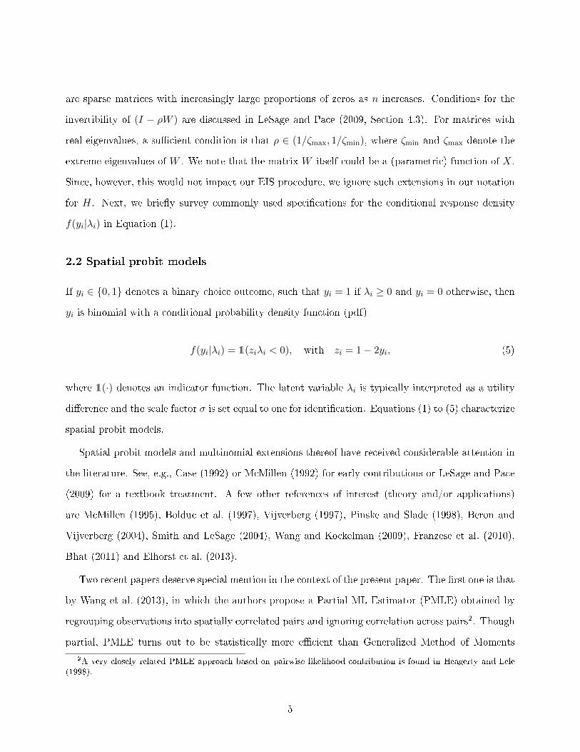
The e�ect of such a permutation is illustrated in Figure 1 (right panel) where we plot the non-zero

elements of a typical H matrix as shown before permutation in the left panel. The speci�c matrix

we use contains 99.7% zero elements and is constructed in the same way as those we use for our MC

study (Section 3.4) and spatial applications (Section 4).

As we shall see in the next section, the combination of sparse factorization of f(u) in Lemma 1

and SAMD permutation allows for fast sparse matrix operations not only for likelihood factorization

but also for the complete EIS implementation. This is one of the critical conditions which ensure

that EIS remains computationally feasible even for very large n's.

We conclude this section by mentioning that, while it is the precision matrix H in Equation (3)

that is typically sparse, there exist occasional speci�cations for which it is Σ = H−1 that is sparse.

One example is provided by the spatial moving average process in Anselin (1999) where Σ is de�ned

as

Σ = σ2(I − ρW )(I − ρW )′. (21)

In such cases the factorization of f(u) in Lemma 1 would be reformulated in terms of a recursive

factorization of the sparse Σ matrix.

3.3 EIS spatial kernels and auxiliary regressions

In this section we propose a generic procedure to construct the auxiliary EIS kernels ki in Equation

(13) ought to approximate ϕiχi−1. It applies to the broad class of (high-dimensional) spatial models

introduced in Section 2.1. It only requires that, as function of ui given yi, f(yi|ui) be of the form4

f(yi|ui) ≡ 1(ui ∈ Di) · fi(ui), (22)

where Di denotes the support of ui = λi −mi given yi. As shown in Equation (19), f(ui|u(i+1)) can

be rewritten as a Gaussian kernel in u(i). Thus, it is natural to select for ki a truncated Gaussian

GHK implementation. However, there it is used in order to maximize the sparsity of the Cholesky factor of H.4Our approach trivially covers the more general case where f(yi|ui) =

∑j 1(ui ∈ Dij) · fij(ui) as, for example, in

Equation (8).

13

kernel in u(i), say

ki(u(i); ai) = 1(ui ∈ Di) exp

{−1

2

(u′(i)Piu(i) − 2u′(i)qi + ri + ln(2π)

)}, (23)

with EIS auxiliary parameters ai = (Pi, qi, ri). We note that the dimension of ai is (n− i+ 1)2/2 +

(n − i + 1) + 1. It follows that a brute force approach to the auxiliary EIS regressions in Equation

(16) would require O(n3) operations, which would be computationally prohibitive for large n's.

Our approach combines two critical components in order to reduce the computational burden to

a manageable O(nδ) with δ � 3. One is the use of the sparse likelihood factorization introduced

in Section 3.2. The other one is careful construction of the EIS kernel ki in order to dramatically

reduce the number of parameters in the auxiliary EIS regressions (16). In Lemma 2, we derive the

integrating factor χi of the kernel ki in Equation (23). In Lemma 3, we then present the recursive

derivation of the auxiliary parameters {ai}ni=1. In order to do so, we rely upon the partitioning of Pi

and qi conformably with u′(i) = (ui, u′(i+1)), say

Pi =

(pi11 pi12

pi21 P i22

), qi =

(qi1

qi2

). (24)

Lemma 2. The integrating factor χi of the truncated Gaussian kernel ki in Equation (23) takes

the form of a product of two kernels in u(i+1):

χi(u(i+1); ai) = χ1i (u(i+1); ai) · χ2

i (u(i+1); ai), (25)

where χ1i is a Gaussian kernel in u(i+1) of the form:

χ1i (u(i+1); ai) = exp

{−1

2

(u′(i+1)P

∗i u(i+1) − 2u′(i+1)q

∗i + r∗i

)}, (26)

with

P ∗i = P i22 −pi21p

i12

pi11, q∗i = qi2 −

pi21qi1

pi11, r∗i = ri −

(qi1)2

pi11+ ln pi11, (27)

14

and χ2i is a non-Gaussian kernel that depends only on a scalar linear combination of u(i+1)

χ2i (u(i+1); ai) ≡ χ2

i (νi+1; ai), (28)

with

νi+1 = αi + β′iu(i+1), αi =qi1pi11

, β′i = −pi12

pi11. (29)

Proof: We rely upon the partitioning introduced in Equation (24) in order to partition ki in

Equation (23) into a truncated Gaussian density in ui given νi+1 and a Gaussian kernel in u(i+1).

Standard Gaussian algebra produces the partitioning

ki(u(i); ai) =[χ1i (u(i+1); ai)

] [1(ui ∈ Di)fN (ui|νi+1, 1/p

i11)], (30)

where fN (·|µ,$2) denotes the density of a Gaussian random variable with mean µ and variance $2.

It immediately follows that:

χ2i (νi+1; ai) =

∫1(ui ∈ Di)fN (ui|νi+1, 1/p

i11)dui, (31)

which, as a function of u(i+1), only depends on νi+1. �

Our next step is the actual construction of the kernel ki in Equation (23). Following Equations

(11), (22), (25) and (28), the product ϕiχi−1 to be approximated by ki is given by

ϕi(u(i))χi−1(u(i); ai−1) = 1(ui ∈ Di)[f(ui|u(i+1))χ

1i−1(u(i); ai−1)

] [fi(ui)χ

2i−1(νi; ai−1)

], (32)

where the product fiχ2i−1 is the sole non-Gaussian kernel. Thus, in order to reduce the dimensionality

of the auxiliary EIS regressions (16), we de�ne ki as the (truncated) product of the two Gaussian

kernels in ϕiχi−1 and of an EIS Gaussian kernel approximation to the product fiχ2i−1 (or just f1 for

i = 1, since χ0 ≡ 1).

Thus, for i > 1, the kernel ki in Equation (23) obtains as the following product of three Gaussian

15

kernels:

ki(u(i); ai) = 1(ui ∈ Di)[f(ui|u(i+1))χ

1i−1(u(i); ai−1)

]k2i (ui, νi; a

∗i ), (33)

where k2i denotes a bivariate EIS Gaussian kernel approximation of the product fiχ2i−1 in Equation

(32), which can be written as

k2i (ui, νi; a∗i ) = k2i (ωi; a

∗i ) = exp

{−1

2

(ω′iBiωi − 2ω′ici + di

)}, (34)

with

ωi =

(ui

νi

)= γi + ∆iu(i), γi =

(0

αi−1

), ∆i =

(e′i

β′i−1

), e′i = (1, 0, . . . , 0), (35)

and the EIS regression parameters a∗i = (Bi, ci, di).

For i = 1, we have χ0 ≡ 1 in which case k2i only needs to approximate f1(u1) and can be written

as

k21(u1, ν1; a∗1) = k21(u1; a

∗1) = exp

{−1

2

(b1u

21 − 2c1u1 + d1

)}, (36)

with EIS regression parameter a∗1 = (b1, c1, d1). As we shall see below, similar univariate simpli�ca-

tions apply to the spatial probit model, for which fi(ui) ≡ 1, and to spatial count data models for

which Di ≡ R so that χ2i = 1.

With these de�nitions in place, it is now a simple matter to derive the recursion providing the

EIS parameters {ai}ni=1 since it amounts to combining the three Gaussian kernels in Equation (33).

For the ease of later reference, we regroup these recursion formulas in the following lemma.

Lemma 3. With ki as de�ned in Equation (33), the EIS auxiliary parameters {ai}ni=1 in Equation

(23) obtain through the following recursion:

For i = 1 (ki with only two Gaussian kernels)

P1 = H∗1 + b1e1e′1, q1 = e1c1, r1 = d1 − lnh111. (37)

16

For i > 1 (ki with three Gaussian kernels)

Pi = H∗i + P ∗i−1 + ∆′iBi∆i, (38)

qi = q∗i−1 + ∆′i(ci −Biγi), (39)

ri = r∗i−1 + di + γ′iBiγi − 2γ′ici − lnhi11, (40)

where (P ∗i−1, q∗i−1, r

∗i−1) and (γi,∆i), as de�ned respectively in Equations (27) and (35) are all

functions of ai−1.

We now have all the components in place to present our simpli�ed spatial EIS auxiliary regressions,

the EIS densities, as well as the corresponding EIS weights. Foremost, we note that after elimination

of the common factors in ϕiχi−1 and ki, as given respectively by Equations (32) and (33), the auxiliary

regressions (16) simplify into

a∗i = arg mina∗i

S∑s=1

{ln[fi

(u(s)i

)· χ2

i−1

(ν(s)i ; ai−1

)]− ln k2i

(u(s)i , ν

(s)i ; a∗i

)}2, (41)

where, as in Equation (16), {u(s)}Ss=1 denotes S i.i.d. trajectories drawn from g(u; a). By construction,

the latter factorizes into a sequence of the following conditional densities for ui given u(i+1):

gi(ui|u(i+1), ai) =1(ui ∈ Di) · fN (ui|νi+1, 1/p

i11)

χ2i (νi+1; ai)

. (42)

Accounting for observation i = 1, the corresponding EIS weights in Equation (15) are given by

w(s)(a) =f1(u

(s)1 )

k21(u(s)1 ; a∗1)

n∏i=2

fi(u(s)i )χ2

i−1(ν(s)i ; ai−1)

k2i (ω(s)i ; a∗i )

. (43)

All in all, the sequential construction of the kernels ki, their integrating factors χi and the EIS

densities gi amounts to combine in step i the EIS regression parameters a∗i from Equation (41) with

H∗i in Lemma 1 and the parameters (P ∗i−1, q∗i−1, r

∗i−1, αi−1, βi−1) in order to obtain according to

Lemma 3 the optimal EIS parameters ai = (Pi, qi, ri) as well as the parameters (P ∗i , q∗i , r∗i , αi, βi) in

Lemma 2 for the next step i+ 1.

17

Most importantly, the results we presented in Lemmas 1 to 3 provide the key to a computationally

feasible EIS implementation for high-dimensional spatial models. There are two reasons for this.

Foremost, the sequential computation of the high dimensional (n − i + 1) × (n − i + 1) matrices

(Pi, P∗i ) and (n− i+1) vectors (qi, q

∗i , βi) depend on the �rst row of H∗i and, therefore, fully preserve

their sparsity under the SAMD permutation. This follows from the fact that the SAMD permutation

maximizes the sparsity of the �rst row of H∗i that determines via Pi in Equation (38) the parameters

P ∗i , q∗i , βi in Equations (27) and (29) which in turn are needed to compute for the next step Pi+1

and qi+1. Thus, the recursive computation of all the high-dimensional auxiliary parameter vectors

required for the spatial EIS can be computed using computationally fast sparse matrix functions.

Moreover, as shown in Equations (34) and (36), the dimension of the auxiliary regressions (41) is

6 for the more general case or 3 in the special cases (i = 1, fi(ui) ≡ 1 or Di ≡ R), irrespective of

n and i. These two key components of our sparse spatial EIS implementation produce computing

times that are O(nδ) with δ � 3, instead of O(n3) that would obtain under brute force EIS.

We mentioned earlier that the EIS auxiliary regressions in Equation (41) have to be iterated since

the trajectories {u(s)} are to be drawn from g(u; a) itself. In practice, this requires constructing

an initial a[0] from initial values for {a∗i }ni=1 and then for iteration j = 1, . . . J , using draws from

g(u; a[j−1]) to compute a new a[j]. Actually, only the �rst few iterations produce signi�cant MC

variance reductions. Thus, we typically preset J at a low �xed number, say from 3 to 5. As for

a[0], it can generally obtained by means of a local Taylor-series approximation to the target fiχ2i to

produce initial values for a∗i , or even by setting a∗i = 0.

In conclusion of this generic presentation, we provide next a pseudo-code summary of the spa-

tial EIS algorithm. Full MATLAB codes are available at http://www.wisostat.uni-koeln.de/index.

php?id=27287.

18

Spatial EIS algorithm

(i) Use CRNs to generate S new i.i.d. trajectories {u(s)} from g(u|a[j−1]), where

a[j−1] = (a[j−1]1 , . . . , a

[j−1]n ).

(ii) (initialization): set P ∗0 = 0, q∗0 = 0, r∗0 = 0, α0 = 0, β0 = 0.

(iii) For i = 1

− run the EIS regression as given by Equations (36) and (41) to obtain a∗1;

− use Equation (37) to compute a[j]1 = (P1, q1, r1);

− use Equations (27) and (29) to compute (P ∗1 , q∗1, r∗1, α1, β1) and pass them to

step i = 2.

For i : 2→ n

− run the EIS regression as given by Equations (34) and (41) to obtain a∗i ;

− use Equations (38) to (40) to compute a[j]i = (Pi, qi, ri);

− use Equations (27) and (29) to compute (P ∗i , q∗i , r∗i , αi, βi) and pass them to

step i+ 1.

(iv) If j ≥ J , then stop and set a = a[J ], else, j → j + 1 and rerun.

After iteration J , the EIS likelihood estimate is computed from Equations (15) and (43).

3.4 Spatial probit model

Under the spatial probit models, the two factors in the measurement density in Equation (22) are

given by

1(ui ∈ Di) = 1(ziui ≤ −zimi), fi(ui) ≡ 1. (44)

It follows that the integrating factor in Equation (31) is given by

χ2i (νi+1; ai) = Φ(−zi

√pi11[mi + νi+1]), (45)

19

where Φ denotes the cdf of a standard normal. For ease of comparison with GHK it proves convenient

to rede�ne accordingly αi and βi in Equation (29) as

αi = −zi√pi11(mi +

qi1pi11

), β′i = zipi12√pi11

, (46)

so that χ2i (νi+1, ai) = Φ(νi+1). Moreover, since fi(ui) ≡ 1, ln k2i in Equation (34) only needs to

approximate ln Φ(νi). This implies the following simpli�cations of the spatial EIS algorithm. For

i = 1 with χ20 ≡ 1 and ln f1 ≡ 0, we have a∗1 = 0 in Equation (36) and k1 ≡ ϕ1χ0 (yielding a perfect

�t). For i > 1, the auxiliary kernel k2i in Equation (34) only depends on νi and Equations (34), (35)

and (37)-(40) simplify accordingly into

k2i (ui, νi; a∗i ) = k2i (νi; a

∗i ) = exp

{−1

2

(biν

2i − 2ciνi + di

)}, (47)

γi =

(0

αi−1

), ∆i =

(0

β′i−1

), (48)

Pi = H∗i + P ∗i−1 + biβi−1β′i−1, P1 = H∗1 , (49)

qi = q∗i−1 + (ci − biαi−1)βi−1, q1 = 0, (50)

ri = r∗i−1 + di + biα2i−1 − 2αi−1ci − lnhi11, r1 = − lnh111, (51)

and the EIS weights in Equation (43) are then given by

w(s)(a) =n∏i=2

Φ(ν(s)i )

exp{−12(bi[ν

(s)i ]2 − 2ciν

(s)i + di)}

. (52)

As mentioned above, our EIS procedure covers GHK as a special case. Speci�cally, the IS density

kernels under GHK are de�ned as

ki(u(i); ·) = ϕi(u(i)) = 1(ziui ≤ −zimi) · f(ui|u(i+1)), (53)

20

with integrating factor χi(νi+1, ·) = Φ(νi+1). This is equivalent to setting k2i ≡ 1 with a∗i =

(bi, ci, di) = 0 in Equations (47)-(52). In particular, the IS weights in Equation (52) simplify into

w(s) =n∏i=2

Φ(ν(s)i ), (54)

where {ν(s)i } are drawn from the sequential GHK-IS truncated Gaussian densities associated with

the kernels in Equation (53). Since a∗i = 0 is generally EIS-suboptimal, it immediately follows that

GHK is numerically less e�cient than EIS. See Liesenfeld and Richard (2010) for a low-dimensional

application (for which sparse matrix operations are not required). In Section 3.6 below, we provide

a high-dimensional comparison of the relative numerical e�ciencies of GHK and EIS, which is trivial

since we initialize EIS with the GHK sampler by setting a∗i = 0 to obtain the initial EIS auxiliary

parameters a[0]. We note that our GHK implementation is directly comparable to those of Beron

and Vijverberg (2004) and Pace and LeSage (2011), though the latter relies upon sparse Cholesky

factorizations of H, instead of the EIS procedure described above.

3.5 Spatial Poisson model

Under the Possion model the measurement density as given by Equation (22) consists of

1(ui ∈ Di) ≡ 1, fi(ui) = f(yi|ui) =1

yi!exp{yi(mi + ui)− exp(mi + ui)}. (55)

Therefore, χ2i ≡ 1 in Equation (28). It follows from Equation (41) that for i = 1, . . . , n we only have

to EIS approximate ln f(yi|ui) by a univariate (log)kernel ln k2i (ui; a∗i ). Thus Equations (34), (35),

and (38)-(40) simplify accordingly into

k2i (ui, νi; a∗i ) = k2i (ui; a

∗i ) = exp

{−1

2

(biu

2i − 2ciui + di

)}, (56)

γi = 0, ∆i =

(e′i

0

), (57)

Pi = H∗i + P ∗i−1 + bieie′i, qi = q∗i−1 + ciei, ri = r∗i−1 + di − lnhi11. (58)

21

The corresponding EIS weights in Equation (43) are then given by

w(s)(a) =n∏i=1

exp{yi(mi + u(s)i )− exp(mi + u

(s)i )}/yi!

exp{−12(bi[u

(s)i ]2 − 2ciu

(s)i + di)}

. (59)

Since the EIS regressions only require approximating ln f(yi|ui) by ln k2i (ui; a∗i ), it immediately

follows that we can directly construct the joint EIS density from Equations (12), (13), (33) and (56)

as

g(u; a) =f(u)

∏ni=1 k

2i (ui; a

∗i )

χn(an), (60)

where

χn(an) =

∫Rn

f(u)

n∏i=1

k2i (ui; a∗i )du (61)

obtains directly using standard Gaussian algebra since the integrand in Equation (61) represents

an untruncated Gaussian kernel in u. This construction of the joint EIS density in a single step

eliminates sequential combination of large matrices and reduces accordingly the computing times (by

a factor of 45 in the application presented in Section 4 below).

Replacing the conditional Poisson density in Equation (6) by the conditional Negbin density

in Equation (7), only requires modifying accordingly the dependent variable ln f(yi|ui) in the EIS

auxiliary regressions.

3.6 Censored Data

Under censoring as de�ned by Equation (8), the pdf for censored data is of the generic form given

by Equation (22) where Di can represent an arbitrary censoring interval for observation i. It follows

that k2i in Equation (34) e�ectively depends on both ui and νi so that the auxiliary EIS parameter

a∗i is now 6-dimensional. Thus, our generic EIS algorithm as described in Section 3.3 immediately

applies to a wide range of spatial models for censored data.

22

4. Monte Carlo Study

In this section, we conduct a MC analysis of the statistical and numerical properties of ML-EIS

estimates for spatial probit and Poisson models. We consider both the SAL (A4.1) and the SAE

(A4.2) speci�cations introduced in Equation (4), where the regression function Xβ for unit i is

speci�ed as

x′iβ = β0 + β1xi. (62)

The regressors xi are assumed to be i.i.d. uniform random variables on the interval (−3, 4) for the

probit models, and on the interval (0, 1) for the Poisson models. Following LeSage and Pace (2009,

Chap. 4.11), we construct the spatial weight matrix W by simulating a pair of coordinates from

a uniform-(0, 1)2 distribution for each spatial unit i. The points associated with those coordinates

are then transformed into a spatial weight matrix W assigning six neighbors to each unit by using

a Delaunay triangulation carried out with the function fasymneighbors2.m in Kelly Pace's spatial

statistics toolbox for MATLAB 2.0 (http://www.spatial-statistics.com). Finally, the spatial weight

matrix is row-standardized.

The parameter values for the four model speci�cations are selected as follows: For the probit

models we set the regression parameters at (β0, β1) = (−1.5, 3) and for the Poisson models at

(β0, β1, σ) = (−0.25, 0.8, 0.3), where σ is the scale parameter in Equation (3) (for the probit models

it is set equal to one to ensure identi�cation). For all four speci�cations we vary the degree of

spatial correlation by taking ρ = 0.75 or ρ = 0.85. We consider di�erent sample sizes ranging

from a moderate n = 100 to a fairly large n = 5000. We only report the results for n = 5000,

which represents a compromise between our interest in large data sets and the need to conduct an

extended MC analysis. We also ran a few tries with n = 50, 000 in order to con�rm the feasibility of

our approach for very large sample sizes and to verify that computing times are indeed O(nδ) with

δ � 3.

Using the Data-Generating Processes (DGPs) we just described we construct two di�erent MC

sampling distributions for the ML-EIS estimators. One is the conventional (�nite-sample) statistical

distribution (used for likelihood-based inference) and the other is the numerical distribution used

23

to assess numerical accuracy (see, e.g., Richard and Zhang, 2007). The statistical distribution of

the ML-EIS estimator is obtained by repeating the ML-EIS estimation for 50 di�erent data sets

using a single set of CRNs for EIS. In contrast, the numerical properties of the ML-EIS estimates as

MC approximations to the true but infeasible ML estimates are analyzed by repeating the ML-EIS

estimation for a given data set using 50 di�erent sets of CRNs. Clearly, reliable statistical inference

requires that numerical biases and standard deviations be negligible relative to statistical standard

deviations.

As explained in Section 3.4, we use GHK to initialize our EIS procedure for spatial probit models.

This enables us to trivially compare the statistical and numerical properties of ML-GHK and ML-

EIS estimates for these models. Unfortunately, no such direct ML competitor is readily available for

spatial count models.

ML-EIS estimates are computed using simulation sample size S = 20 and J = 3 EIS iterations.

For the probit models with n = 5000, a single likelihood EIS evaluation using a MATLAB code

takes of the order of 45 s on a Intel i7 Core computer with 2.67 GHz. The corresponding computing

time for the Poisson models is only 1 s, as we rely upon the joint EIS implementation described in

Equation (60). For the probit models GHK is much faster than EIS (by an approximate factor of

25), since it does not require (iterated) auxiliary regressions, but is also signi�cantly less accurate.

Thus, we compare EIS based on S = 20 with GHK using S = 500 in order to approximately equate

computing times. For all ML estimations we use the BFGS optimizer.

4.1 Spatial probit models

The main results of our four MC experiments for the spatial probit model are reported in Table

1. The DGP parameter values are listed in column 1. Statistical means, standard deviations and

Root Mean Squared Errors (RMSEs) for ML-GHK and ML-EIS are reported in columns 2 and 3,

respectively. 'True' ML estimates, de�ned as ML-EIS estimates with S = 1000 are listed in column

5. Numerical means, standard deviations and RMSEs for ML-GHK and ML-EIS are listed in column

6 and 7, respectively.

Our main �nding is that the ML-EIS estimates are statistically virtually unbiased and numerically

24

highly accurate. The ratios between statistical and numerical standard errors range roughly from

20 to 100. Thus, statistical inference based on ML-EIS is largely una�ected by numerical errors and

fully reliable.

In sharp contrast, ML-GHK estimates are statistically signi�cantly biased with RMSEs 2 to

23 times larger than those of ML-EIS. Foremost, ML-GHK estimates are numerically considerably

less accurate than their ML-EIS counterparts with RMSEs ratios ranging from 90 to 384. Clearly,

statistical results obtained by ML-GHK are subject to large numerical errors and are essentially

unreliable. In order to match EIS-ML numerical accuracy, GHK would require a prohibitively large

simulation sample size S.

The explanation for such poor numerical performance is that the GHK-IS density g(u; .) obtained

from the kernels in Equation (53) represents a very poor global approximation to the high-dimensional

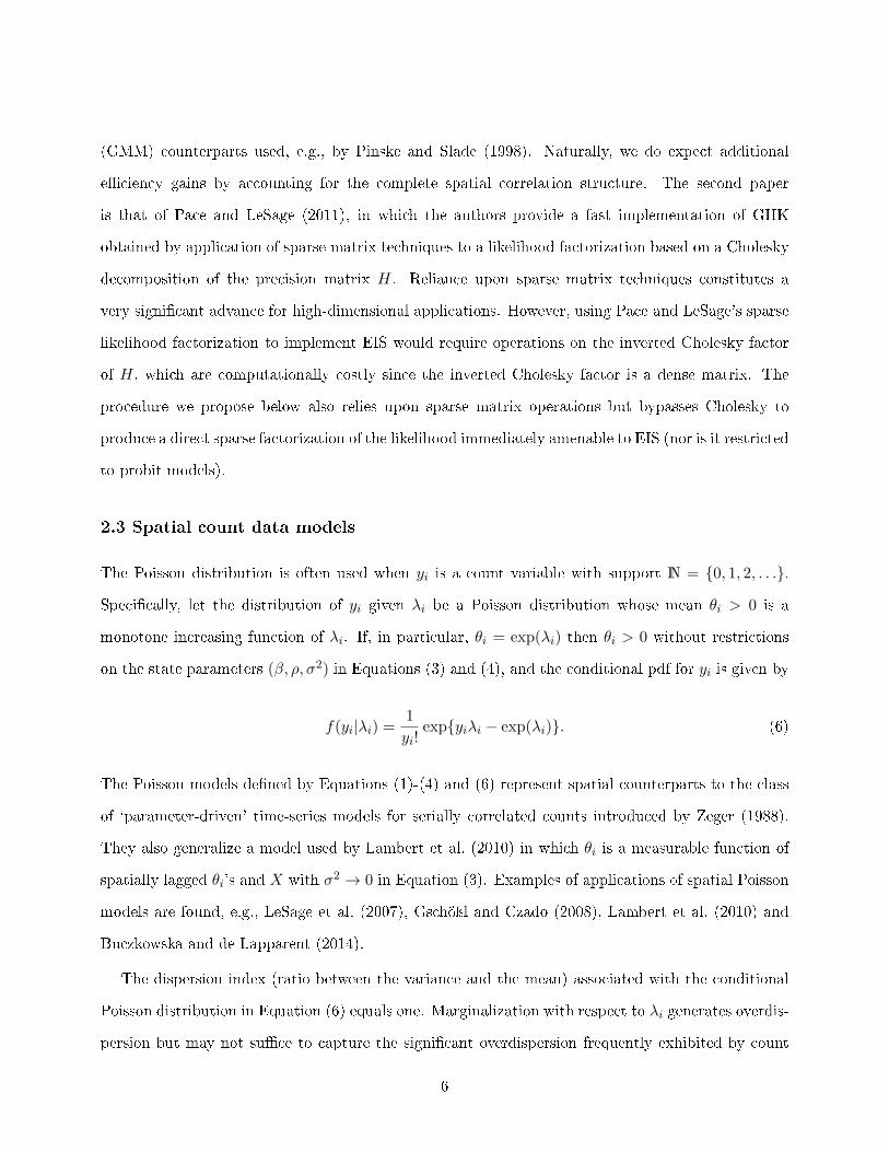
target∏i ϕi(u(i)). In order to verify this conjecture we present in Figure 2 histograms of the nor-

malized IS weights ω(s) = ω(s)/∑S

s=1 ω(s) for both EIS and GHK, as de�ned in Equations (52) and

(54), respectively. A perfect IS �t would imply that ω(s) = 1/S, ∀s. The histogram of the normalized

GHK-IS weights exhibits extreme skewness with only 2 out of 500 weights that are e�ectively larger

than zero (0.39 and 0.61). The corresponding histogram for the 500 EIS weights is clearly much

better behaved. Our results are consistent with the �ndings of Pace and LeSage (2011) who also

report an extremely skewed distribution of the GHK-IS weights for n = 100, 000 and S = 30. As

a remedy, they propose to replace the GHK likelihood estimate L = χn · 1S

∑Ss=1

∏ni=2 Φ(ν

(s)i ), as

de�ned by Equations (15) and (54), by the alternative estimate L = χn ·∏ni=2[

1S

∑Ss=1 Φ(ν

(s)i )] which

would remain unbiased if the terms of the sequence {Φ(ν(s)i )}ni=2 were mutually uncorrelated. This

condition, however, would need to be checked empirically for each application.

The results of the four MC experiments obtained by using Page and LeSage's modi�ed MC

likelihood estimate L using S = 500 (GHKPL) are reported in columns 4 and 8 of Table 1. They

reveal that ML-GHKPL performs better than the standard ML-GHK in terms of statistical and

numerical properties but remains dominated by ML-EIS with statistical RMSEs ratios ranging from

1 to 1.5 and numerical RMSEs ratios between 4 and 53.

25

4.2 Spatial Poisson models

The MC results for the Spatial SAL and SAE Poisson model are reported in Table 2. They show

that for all four DGPs and for all parameters, the ML-EIS estimators are virtually unbiased with

S as low as 20. Numerical accuracy is high with means that are close to the `true' ML values and

standard deviations that are signi�cantly smaller than their statistical counterparts.

We conclude that likelihood based inference results obtained by spatial EIS for probit and Poisson

models with n = 5, 000 are numerically very accurate even with MC sample sizes as low as 20. As

for the dependence on n, we have run experiments with larger n's (up to 50,000) and have found

computing times of the order of O(n1.5) for the probit models and virtually O(n) for the Poisson

models under the simpli�ed implementation according to Equation (60).

5. Empirical Applications

In this section we present two empirical applications relying upon ML-EIS. One uses a spatial probit

model for voting decisions at the county level in the 1996 US presidential election, and the other

a spatial count model (Poisson and Negbin) for �rm location decisions in US manufacturing. Both

models rely upon the SAL speci�cation A4.1 in Equation (4).

5.1 Spatial probit for the 1996 US presidential election

We use a SAL probit to model the voting decisions of the n = 3, 110 US counties in the 1996

US presidential election. The dependent variable yi equals one if the Democratic Candidate Bill

Clinton won the majority in county i and zero if the Republican candidate Bob Dole won. The SAL

speci�cation is the same as that used for the MC study in Section 4, expect that xi in Equation

(62) is now a vector which includes the log urban population and the following four educational

level variables (expressed as a proportion of the county population): some years at college, associate

degrees, college degrees and graduate or professional degrees. The data are taken from LeSage's

spatial econometric toolbox (http://www.spatial-econometrics.com).

Spatial dependence re�ects the fact that voters from neighboring counties tend to exhibit similar

26

voting patterns. As was the case for our MC study, we constructW using the geographical coordinates

(latitude and longitude) of the counties and transforming them by a Delaunay triangulation in order

to assign to each county its six `closest' neighbors. As in Section 4.1, the ML-EIS parameter estimates

rely upon simulation sample size S = 20 and J = 3 EIS iterations, while ML-GHK uses S = 500.

Following, e.g., Beron and Vijverberg (2004), we also compute average marginal e�ects de�ned

as:

1

n

n∑i=1

∂prob(yi = 1|X,W )

∂xi=

1

n

n∑i=1

φ(h12i [vi1x

′1β + · · ·+ vinx

′nβ]) · h

12i viiβ, (63)

where φ(·) denotes the standardized normal density function, vij is the element (i, j) of the matrix

V = (I − ρW )−1, and hi is the precision of the marginal distribution of the error ui. These marginal

e�ects account for both the direct impact on λi of a change in x′iβ and its indirect impact through

the spatial interdependence re�ected by the matrix V .

The results are reported in Table 3. Asymptotic (statistical) standard deviations are derived from

a numerical approximation of the Hessian. Numerical standard deviations are based upon 50 ML-EIS

estimations using di�erent CRNs. They con�rm our earlier �nding that ML-EIS is numerically far

more accurate than ML-GHK. Our ML-EIS estimate of ρ is highly signi�cant and implies strong

spatial dependence across neighboring counties, in line with the Bayesian MCMC results obtained by

LeSage and Pace (2009, Table 10.3) for the 2000 US presidential election. Our results also con�rm

the downward bias of the ML-GHK estimates of ρ, as already observed in our MC study. The

ML-EIS estimates of the β parameters and the corresponding marginal e�ects are systematically

lower in absolute value than their ML-GHK counterparts. Under ML-EIS only two variables have

a signi�cant impact: negative for some college and positive for graduate/professional degree. Thus,

higher education levels play in favor of Clinton. Finally, ML-EIS produces a signi�cantly higher value

than ML-GHK for the maximized log likelihood. This con�rms a negative bias we had previously

observed when comparing GHK with `brute force' EIS for n = 20 in Liesenfeld and Richard (2010).

27

5.2 Spatial count model for US �rms location choices

In this section we apply the spatial count models (Poisson and Negbin) introduced in Section 2.3 to

US �rm births (start-ups) at the county level (n = 3, 078) during the period 2000-2004. We rely upon

a data set from Lambert et al. (2010, Section 6), hereafter LBF, who applied a two-step Limited-

Information ML (LIML) procedure to estimate an `observation-driven' version of the SAL-Poisson

model introduced in Section 2.3, with σ → 0 in Equation (3). Instead we apply Full-Information ML

(FIML) to the `parameter-driven' version (σ > 0) of that model. Spatial correlation is expected to

re�ect such factors as industry clustering and regional economic development policies. We refer the

reader to LBF for an insightful discussion of the covariates used in the SAL regression.

The dependent variable yi is de�ned as the cumulative number of new single-unit start-ups from

2000 to 2004. Following LBF we construct the weight matrix W using the Delaunay triangulation

algorithm to assign eight neighbors to each county. The set of explanatory variables consists of

location factors of the counties related to agglomeration economies, market structure, labor mar-

ket, infrastructure, and the �scal policy regime. The agglomeration variables are the manufacturing

share of employment (Msemp), total establishment density (Tfdens), percentage of manufacturing

establishments with less than 10 (Pelt10), and more than 100 employees (Pemt100). The market

structure variables are median household income (Mhhi), population (Pop), and the share of workers

in creative occupations (Cclass). Properties of the regional labor markets are measured by the av-

erage wage per job (Awage), net �ows of wages per commuter (Net�ow), Unemployment rate (Uer),

percentage of adults with associate degree (Pedas). The variables characterizing the regional infras-

tructure are the public road density (Proad), interstate highway miles (Interst), public expenditures

on highways per capita (Hwypc), the percentage of farmland to total county area (Avland). The

�scal policy variables are a tax business climate index (Bci), per capita government expenditures on

education (Educpc). Also included in the set of regressors are dummy variables identifying counties

as belonging to metropolitan (Metro ) or micropolitan (Micro) areas.

Our SAL-Poisson ML-EIS estimates obtained with a MC sample size S = 20 and J = 3 EIS

iterations are reported in the left panel of Table 4. They are mostly in line with those reported in

LBF's Table 6, though generally with signi�cantly smaller statistical standard deviations, as expected

28

from using FIML instead of LIML. We observe signi�cant sign changes for only three covariates

Pelt10, Awage and Net�ow. Three other parameters have the same sign but are, nevertheless,

signi�cantly di�erent (based on the FIML standard deviations): Pemt100, Pop and Pedas. Overall

our results con�rm LBF's conclusion that counties with agglomeration economies, labor availability,

low costs for labor, availability of skilled labor, a business-friendly infrastructure and �scal policy

were more likely to attract new start-ups. However, there are two key di�erences with LBF's results.

One is that we �nd a signi�cantly higher estimate of the spatial correlation parameter ρ: 0.514

(0.018) instead of 0.181 (0.062). The other is that our estimate of σ is 0.697 (0.013) and implies a

strong rejection of LBF's speci�cation where σ is set equal to zero.

Since counts frequently exhibit over-dispersion, we also estimated a SAL-Negbin model version

that, as explained above, only requires minor modi�cations of the baseline spatial-EIS algorithm. The

ML-EIS Negbin results are reported in the right panel of Table 4. The estimates of the regression

coe�cients are largely in agreement with those obtained under the Poisson speci�cation, with only

one statistically signi�cant sign di�erence for Mhhi. The dispersion parameter estimate of s equals

2.902 (0.204) and is statistically signi�cantly smaller than in�nity, implying rejection of the Poisson

model, as further con�rmed by a large log-likelihood di�erence of 395. The Negbin estimate of σ is

signi�cantly lower (0.261 instead of 0.697) but this was to be expected from the substitution of an

over-dispersed Negbin for the Poisson. Last but not least, we also �nd a signi�cantly lower estimate

of ρ (0.321 instead of 0.514). These di�erences suggest that a signi�cant part of the variation in the

�rm-birth events across counties, that was attributed to shocks with global spatial feedback and feed-

forward transmission between locations under the Poisson model, is interpreted as conditional over-

dispersion together with lesser spatial transmission under the Negbin model. Numerical accuracy is

good for the Poisson model and excellent for the Negbin speci�cation. While we could easily improve

the numerical accuracy of the Poisson estimates by increasing S, we decided there was little reason

for doing so, since the Poisson model is strongly rejected against the Negbin model.

29

6. Conclusions

We have proposed a generic EIS-based procedure for numerically accurate likelihood evaluation of a

broad class of high-dimensional spatial latent Gaussian models with non-Gaussian response variables

(discrete choices, counts, truncation, censoring and sample selection). Our algorithm consists of an

original and powerful combination of sparse-matrix techniques and EIS. Its two key features are: (i)

a novel forward-recursive implementation of EIS that is speci�cally constructed in such a way that it

preserves the sparsity of large (auxiliary) precision matrices throughout the entire recursive sequence

so that all high-dimensional EIS matrix operations can be performed using computationally fast

sparse matrix functions; and (ii) a selection of auxiliary importance sampling kernels that produces

low-dimensional auxiliary EIS regressions, irrespectively of the data size n. The combination of these

two features produces an algorithm that remains computationally feasible for large sample sizes n,

with computing times of O(nδ) with δ � 3 (δ ' 1.5 for probit applications and δ ' 1 for Poisson

and Negbin models with n as large as 5,000, or even 50,000 in test trials).

Two empirical applications with sample sizes of the order of 3,000 have illustrated further the full

potential of our spatial EIS procedure for accurate likelihood based inference. While in the paper we

restricted our attention to probit, Poisson and Negbin models, the generic structure of our algorithm,

as presented in Section 3, indicates that it can easily be applied to a much broader class of spatial

models including but not limited to spatial ordered or multinomial probits, spatial tobit models,

spatial truncated and sample selection models. Most importantly, applications to such models would

only require minor adjustments of the baseline spatial EIS implementation presented in Section 3

(essentially adapting the dependent variable in the auxiliary EIS regressions and the corresponding

(E)IS weights).

All in all, our procedure allows for numerically accurate likelihood based inference in a broad class

of high-dimensional spatial latent Gaussian models, a task hitherto considered to be computationally

prohibitive.

30

Acknowledgements

The authors thank Jason Brown for providing the �rm location choice data set used in this paper and

Albrecht Mengel for providing access to the grid computing facilities of the Institute of Statistics and

Econometrics at University of Kiel. R. Liesenfeld and J. Vogler acknowledge support by the Deutsche

Forschungsgemeinschaft (grant LI 901/3-1). For the helpful comments and suggestions they provided

on earlier versions of the paper, we thank seminar and conference participants at the University of

Kiel, University of Cologne, University of Université catholique de Louvain (CORE), 2013 Spatial

Statistics conference (Ohio), the 2013 Econometric Society European Meeting (Gothenburg), the 2013

International Conference on Computational and Financial Econometrics (London), the 2014 World

Conference of the Spatial Econometrics Association (Zürich), the 2014 International Conference on

Computational Statistics (Geneva), the 2014 ERSA Congress (Saint Petersburg), the Statistische

Woche 2014 (Hannover). A former version of this paper circulated under the title `Analysis of

discrete dependent variable models with spatial correlation'.

31

References

Alan, G., Liu, J.W.H., 1981. Computer solution of large sparse positive de�nite systems. Prentice-Hall.

Amestoy, P.R., Davis, T.A., Du�, I.S., 1996. An approximate minimum degree ordering algorithm. SIAM

Journal on Matrix Analysis and Applications 17, 886-905.

Anselin, L., 1999. Spatial Econometrics. University of Texas at Dallas School of Social Sciences: Bruton

Center.

Anselin, L., Florax, R.J.G.M., Rey, S.J., 2010. Advances in Spatial Econometrics: Methodology, Tools and

Applications. Springer.

Ariba, G., 2006. Spatial Econometrics. Springer.

Banerjee, S., Wall, M.M., Carlin, B.P., 2003. Frailty modeling for spatially correlated survival data, with

applications to infant mortality in Minnesota. Biostatistics 4, 123�142.

Bauwens, L., Galli, F., 2009. E�cient importance sampling for ML estimation of SCD models. Computa-

tional Statistics and Data Analysis 53, 1974�1992.

Beron, K.J., Vijverberg, W.P.M., 2004. Probit a spatial context: A Monte-Carlo analysis. In Anselin, L.,

Florax, R., Rey, S.J. (eds), Advances in Spatial Econometrics: Methodology, Tools and Applications.

Springer-Verlag, Berlin, 169�195.

Bhat, C.R., 2011. The maximum approximated composite marginal likelihood (MACML) estimation of

multinomial probit-based unordered response choice models. Transportation Research Part B: Method-

ological 45, 923�939.

Bolduc, D., Fortin, B., Gordon, S., 1997. Multinomial probit estimation of spatially interdependent choices:

An empirical comparison of two new techniques. International Regional Science Review 20, 77�101.

Buczkowska, S., de Lapparent, M., 2014. Location choices of newly created establishments: Spatial patterns

at the aggregate level. Regional Science and Urban Economics 48, 68�81.

Case, A.C., 1992. Neighborhood in�uence and technological change. Regional Science and Urban Economics

22, 491�508.

DeJong, D.N., Liesenfeld, R., Moura, G.V., Richard, J.-F., Dharmarajan, H., 2013. E�cient likelihood

evaluation of state-space representations. Reviews of Economic Studies 80, 538�567.

32

Elhorst, P., Heijnen, P., Samarina, A., Jacobs, J., 2013. State transfers at di�erent moments in time: A

spatial probit approach. Working paper 13006-EEF, University of Groningen.

Fischer, M.M., Nijkamp, P., 2014. Handbook of Regional Science. Springer-Verlag, Berlin.

Franzese, R.J., Hays, J.C., Schae�er, L.M., 2010. Spatial, temporal, and spatiotemporal autoregressive probit

models of binary outcomes: Estimation, interpretation, and presentation. Working paper, University

of Michigan, Ann Arbor.

Geweke, J., 1991. E�cient Simulation from the Multivariate Normal and Student-t Distributions Subject

to Linear Constraints and the Evaluation of Constraint Probabilities. University of Minnesota Depart-

ment of Economics; Published in: Computer Science and Statistics: Proceedings of the Twenty-Third

Symposium on the Interface, 571�578.

Gourieroux, C., Monfort, A., 1996. Simulation-based Econometric Methods. Oxford University Press.

Gschlöÿl, S., Czado, C., 2008. Does a Gibbs sampler approach to spatial Poisson regression models outper-

form a single site MH sampler? Computational Statistics and Data Analysis 52, 4184�4202.

Hafner, C.M., Manner, H., 2012. Dynamic stochastic copula models: estimation, inference and applications.

Journal of Applied Econometrics 27, 269�295.

Hajivassiliou, V., 1990. Smooth simulation estimation of panel data LDV models. Mimeo Yale University.

Heagerty, P.J., Lele, S.R., 1998. A composite likelihood approach to binary spatial data. Journal of the

American Statistical Association 93, 1099�1111.

Jung, R.C., Liesenfeld, R., Richard, J.-F., 2011. Dynamic factor models for multivariate count data: An

application to stock-market trading activity. Journal of Business and Economic Statistics 29, 73�85.

Keane, M., 1994. A computationally practical simulation estimator for panel data. Econometrica 62, 95�116.

Kleppe, T.S., Skaug, H.J., 2012. Fitting general stochastic volatility models using Laplace accelerated

sequential importance sampling. Computational Statistics and Data Analysis 56, 3105�3119.

Kneib, T., 2005. Geoadditive hazard regression for interval censored survival times. Working Paper 447,

Sonderforschungsbereich 386, Ludwig-Maximilians-Universität München.

Koopman, S.J., Lucas, A., Scharth, M., 2014. Numerically accelerated importance sampling for nonlinear

non-Gaussian state space models. Journal of Business and Economic Statistic, forthcoming.

Lambert, D. M., Brown, J.P., Florax, R.J.G.M., 2010. A two-step estimator for spatial lag model of counts:

Theory, small sample performance and application. Regional Science and Urban Economics 40, 241�252.

33

Lee, L.-F., 1997. Simulated maximum likelihood estimation of dynamic discrete choice models � some Monte

Carlo results. Journal of Econometrics 82, 1�35.

LeSage, J.P., Fischer, M.M., Scherngell, T., 2007. Knowledge spillovers across Europe: Evidence from a

Poisson spatial interaction model with spatial e�ects. Papers in Regional Science 86, 393�422.

LeSage, J.P., Pace, R.K., 2009. Introduction to Spatial Econometrics. CRC Press, Taylor and Francis

Group.

Liesenfeld, R., Moura, G.V., Richard, J.-F., 2010. Determinants and dynamics of current account reversals:

An empirical analysis. Oxford Bulletin of Economics and Statistics 72, 486�517.

Liesenfeld, R., Richard, J.-F., 2003. Univariate and multivariate stochastic volatility models: Estimation

and diagnostics. Journal of Empirical Finance 10, 505�531.

Liesenfeld, R., Richard, J.-F., 2006. Classical and Bayesian analysis of univariate and multivariate stochastic

volatility models. Econometric Reviews 25, 335�360.

Liesenfeld, R., Richard, J.-F., 2008. Improving MCMC using e�cient importance sampling. Computational

Statistics and Data Analysis 53, 272�288.

Liesenfeld, R., Richard, J.-F., 2010. E�cient estimation of probit models with correlated errors. Journal of

Econometrics 156, 367�376.

McMillen, D.P., 1992. Probit with spatial autocorrelation. Journal of Regional Science 32, 335�348.

McMillen, D.P., 1995. Spatial e�ects in probit models: A Monte Carlo investigation. In Anselin, L., Florax,

R. (eds.), New Directions in Spatial Econometrics. Springer-Verlag, Berlin, 169�195.

Militino, A.F., Ugarte, M.D., 1999. Analyzing censored spatial data. Mathematical Geology 31, 551�561.

Pace, R.K., 2014. Maximum likelihood estimation. In Fischer, M.M., Nijkamp, P. (eds.), Handbook of

Regional Science. Springer-Verlag, Berlin, 1553�1569.

Pace, R.K., Barry, R., 1997. Quick computation of regressions with a spatially autoregressive dependent

variable. Geographical Analysis 29, 232�247.

Pace, R.K., LeSage, J.P., 2011. Fast simulated maximum likelihood estimation of the spatial probit model

capable of handling large samples. Working paper, Louisiana State University, Baton Rouge.

Pastorello, S., Rossi, E., 2010. E�cient importance sampling maximum likelihood estimation of stochastic

di�erential equations. Computational Statistics and Data Analysis 54, 2753�2762.

34

Pinske, J., Slade, M.E., 1998. Contracting in space: An application of spatial statistics to discrete choice

models. Journal of Econometrics 85, 125�154.

Richard, J.-F., Zhang, W., 2007. E�cient high-dimensional importance sampling. Journal of Econometrics

141, 1385�1411.

Rue, H., Martino, S., Chopin, N., 2009. Approximate Bayesian inference for latent Gaussian models by using

integrated nested Laplace approximations. Journal of the Royal Statistical Society, Series B, 319�392.

Scharth, M., Kohn, R., 2013. Particle e�cient importance sampling. Working paper, University of New

South Wales, Australian School of Business.

Smith, T.E., LeSage, J.P., 2004. A Bayesian probit model with spatial dependencies. In LeSage, J.P., Pace,

R.K. (eds.), Advances in Econometrics, Vol. 18, Spatial and Spatiotemporal Econometrics. Elsevier,

127�160.

Toscas, P.J., 2010. Spatial modelling of left censored water quality data. Environmetrics 21, 632�644.

Vijverberg, W.P.M., 1997. Monte Carlo evaluation of multivariate normal probabilities. Journal of Econo-

metrics 76, 281�307.

Wang, H., Iglesias, E.M., Wooldridge, J.M., 2013. Partial maximum likelihood estimation of spatial probit

models. Journal of Econometrics 172, 77�89.

Wang, X., 2014. Limited and censored dependent variable models. In Fischer, M.M., Nijkamp, P. (eds.),

Handbook of Regional Science. Springer-Verlag, Berlin, 1619�1635.

Wang, X., Kockelman, K., 2009. Bayesian inference for ordered response data with a dynamic spatial-ordered

probit model. Journal of Regional Science 49, 877�913.

Winkelmann, R., Boes, S., 2006. Analysis of Microdata. Springer.

Zeger, S.L., 1988. A regression model for time series of counts. Biometrika 75, 621�629.

35

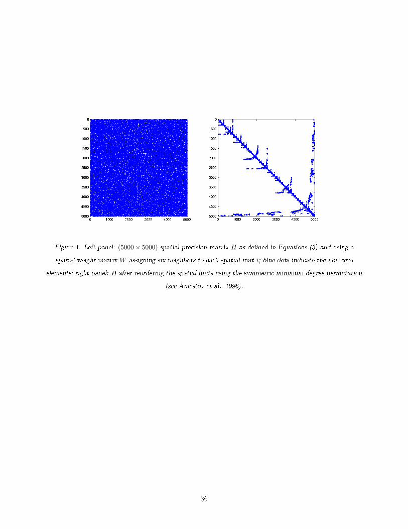
Figure 1. Left panel: (5000× 5000) spatial precision matrix H as de�ned in Equations (3) and using a

spatial weight matrix W assigning six neighbors to each spatial unit i; blue dots indicate the non-zero

elements; right panel: H after reordering the spatial units using the symmetric minimum degree permutation

(see Amestoy et al., 1996).

36

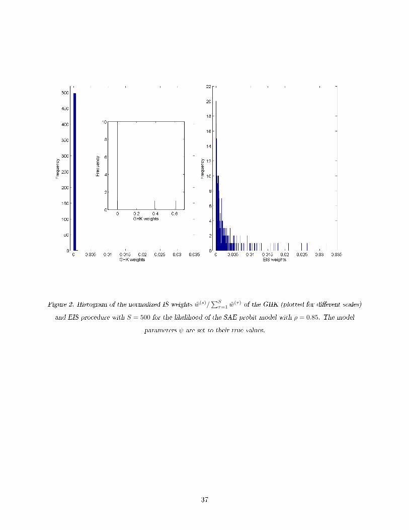
Figure 2. Histogram of the normalized IS weights w(s)/∑Sτ=1 w

(τ) of the GHK (plotted for di�erent scales)

and EIS procedure with S = 500 for the likelihood of the SAE probit model with ρ = 0.85. The model

parameters ψ are set to their true values.

37

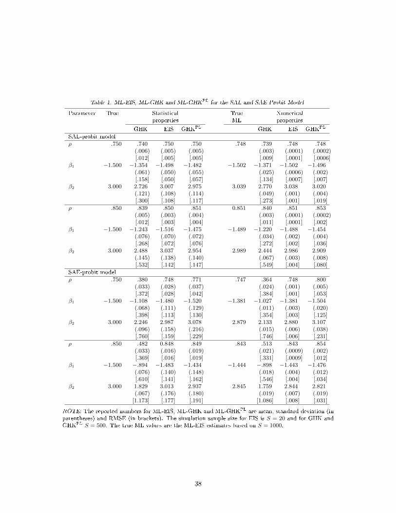
Table 1. ML-EIS, ML-GHK and ML-GHKPL for the SAL and SAE Probit Model

Parameter True Statistical True Numericalproperties ML properties

GHK EIS GHKPL GHK EIS GHKPL

SAL-probit modelρ .750 .740 .750 .750 .748 .739 .748 .748

(.006) (.005) (.005) (.003) (.0001) (.0002)[.012] [.005] [.005] [.009] [.0001] [.0006]

β1 −1.500 −1.354 −1.498 −1.482 −1.502 −1.371 −1.502 −1.496(.061) (.050) (.055) (.025) (.0006) (.002)[.158] [.050] [.057] [.134] [.0007] [.007]

β2 3.000 2.726 3.007 2.975 3.039 2.770 3.038 3.020(.121) (.108) (.114) (.049) (.001) (.004)[.300] [.108] [.117] [.273] [.001] [.019]

ρ .850 .839 .850 .851 0.851 .840 .851 .853(.005) (.003) (.004) (.003) (.0001) (.0002)[.012] [.003] [.004] [.011] [.0001] [.002]

β1 −1.500 −1.243 −1.516 −1.475 −1.489 −1.220 −1.488 −1.454(.076) (.070) (.072) (.034) (.002) (.004)[.268] [.072] [.076] [.272] [.002] [.036]

β2 3.000 2.488 3.037 2.954 2.989 2.444 2.986 2.909(.145) (.138) (.140) (.067) (.003) (.008)[.532] [.142] [.147] [.549] [.004] [.080]

SAE-probit modelρ .750 .380 .748 .771 .747 .364 .748 .800

(.033) (.028) (.037) (.024) (.001) (.005)[.372] [.028] [.042] [.384] [.001] [.053]

β1 −1.500 −1.108 −1.480 −1.520 −1.381 −1.027 −1.381 −1.504(.068) (.111) (.129) (.011) (.003) (.020)[.398] [.113] [.130] [.354] [.003] [.125]

β2 3.000 2.246 2.987 3.078 2.879 2.133 2.880 3.107(.096) (.158) (.216) (.015) (.006) (.038)[.760] [.159] [.229] [.746] [.006] [.231]

ρ .850 .482 0.848 .849 .843 .513 .843 .854(.033) (.016) (.019) (.021) (.0009) (.002)[.369] [.016] [.019] [.331] [.0009] [.012]

β1 −1.500 −.894 −1.483 −1.434 −1.444 −.898 −1.443 −1.476(.076) (.140) (.148) (.018) (.004) (.012)[.610] [.141] [.162] [.546] [.004] [.034]

β2 3.000 1.829 3.013 2.937 2.845 1.759 2.844 2.821(.067) (.176) (.180) (.019) (.007) (.019)[1.173] [.177] [.191] [1.086] [.008] [.031]

NOTE: The reported numbers for ML-EIS, ML-GHK and ML-GHKPL are mean, standard deviation (inparentheses) and RMSE (in brackets). The simulation sample size for EIS is S = 20 and for GHK andGHKPL S = 500. The true ML values are the ML-EIS estimates based on S = 1000.

38

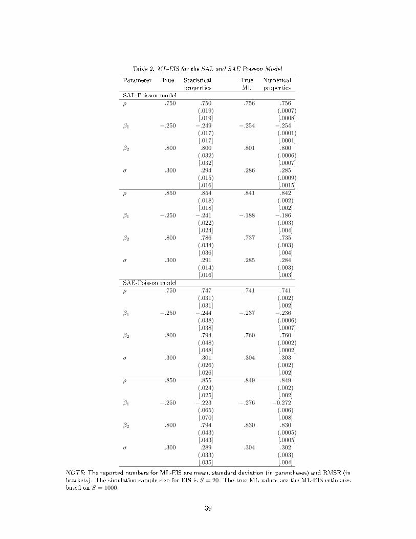
Table 2. ML-EIS for the SAL and SAE Poisson Model

Parameter True Statistical True Numericalproperties ML properties

SAL-Poisson modelρ .750 .750 .756 .756

(.019) (.0007)[.019] [.0008]

β1 −.250 −.249 −.254 −.254(.017) (.0001)[.017] [.0001]

β2 .800 .800 .801 .800(.032) (.0006)[.032] [.0007]

σ .300 .294 .286 .285(.015) (.0009)[.016] [.0015]

ρ .850 .854 .841 .842(.018) (.002)[.018] [.002]

β1 −.250 −.241 −.188 −.186(.022) (.003)[.024] [.004]

β2 .800 .786 .737 .735(.034) (.003)[.036] [.004]

σ .300 .291 .285 .284(.014) (.003)[.016] [.003]

SAE-Poisson modelρ .750 .747 .741 .741

(.031) (.002)[.031] [.002]

β1 −.250 −.244 −.237 −.236(.038) (.0006)[.038] [.0007]

β2 .800 .794 .760 .760(.048) (.0002)[.048] [.0002]

σ .300 .301 .304 .303(.026) (.002)[.026] [.002]

ρ .850 .855 .849 .849(.024) (.002)[.025] [.002]

β1 −.250 −.223 −.276 −0.272(.065) (.006)[.070] [.008]

β2 .800 .794 .830 .830(.043) (.0005)[.043] [.0005]

σ .300 .289 .304 .302(.033) (.003)[.035] [.004]

NOTE: The reported numbers for ML-EIS are mean, standard deviation (in parentheses) and RMSE (inbrackets). The simulation sample size for EIS is S = 20. The true ML values are the ML-EIS estimatesbased on S = 1000.

39

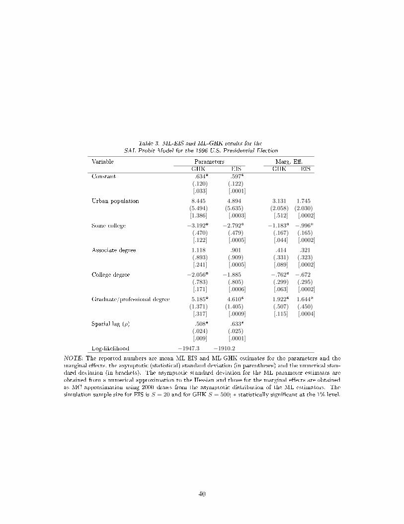
Table 3. ML-EIS and ML-GHK results for the

SAL Probit Model for the 1996 U.S. Presidential Election

Variable Parameters Marg. E�.GHK EIS GHK EIS

Constant .634* .597*(.120) (.122)[.033] [.0001]

Urban population 8.445 4.894 3.131 1.745(5.494) (5.635) (2.058) (2.030)[1.386] [.0003] [.512] [.0002]

Some college −3.192* −2.792* −1.183* −.996*(.470) (.479) (.167) (.165)[.122] [.0005] [.044] [.0002]

Associate degree 1.118 .901 .414 .321(.893) (.909) (.331) (.323)[.241] [.0005] [.089] [.0002]

College degree −2.056* −1.885 −.762* −.672(.783) (.805) (.299) (.295)[.171] [.0006] [.063] [.0002]

Graduate/professional degree 5.185* 4.610* 1.922* 1.644*(1.371) (1.405) (.507) (.450)[.317] [.0009] [.115] [.0004]

Spatial lag (ρ) .508* .633*(.024) (.025)[.009] [.0001]

Log-likelihood −1947.3 −1910.2NOTE: The reported numbers are mean ML-EIS and ML-GHK estimates for the parameters and themarginal e�ects, the asymptotic (statistical) standard deviation (in parentheses) and the numerical stan-dard deviation (in brackets). The asymptotic standard deviation for the ML parameter estimates areobtained from a numerical approximation to the Hessian and those for the marginal e�ects are obtainedas MC approximation using 2000 draws from the asymptotic distribution of the ML estimators. Thesimulation sample size for EIS is S = 20 and for GHK S = 500; ∗ statistically signi�cant at the 1% level.

40

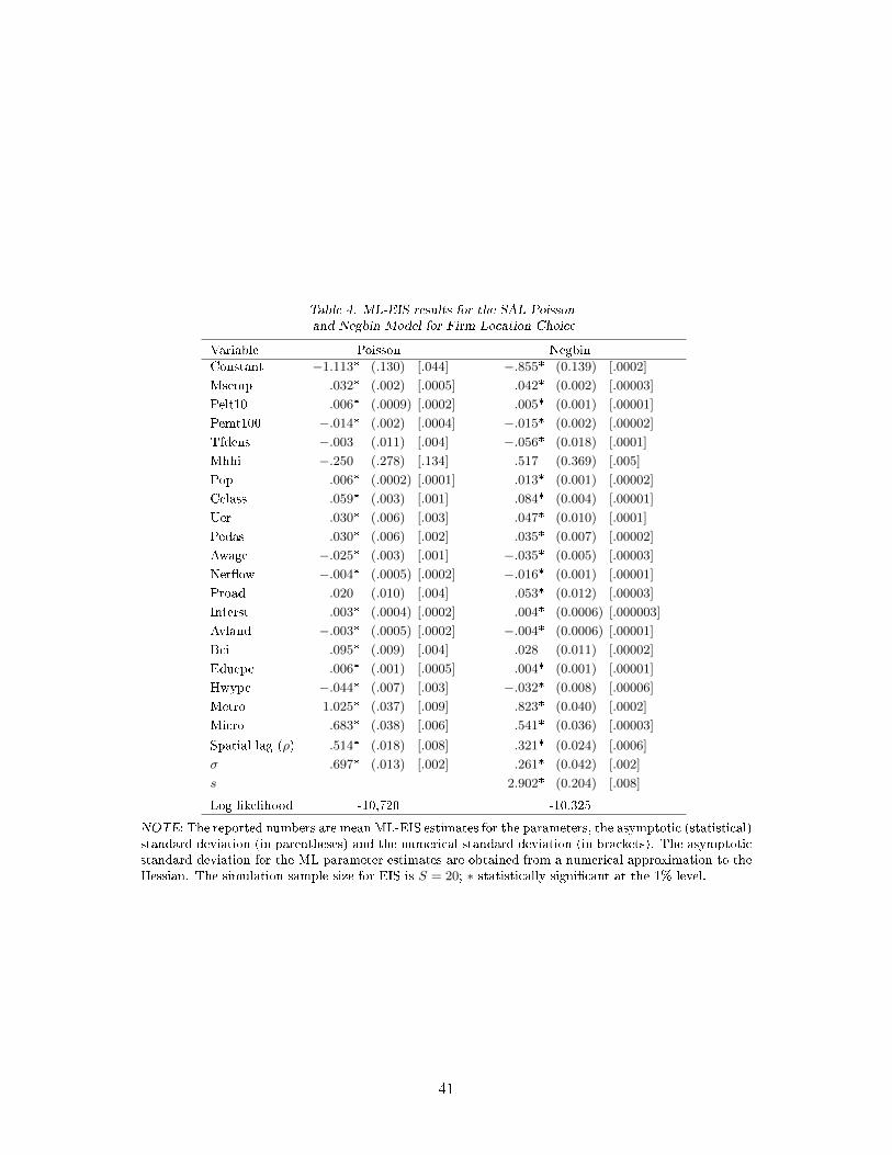
Table 4. ML-EIS results for the SAL Poisson

and Negbin Model for Firm Location Choice

Variable Poisson NegbinConstant −1.113* (.130) [.044] −.855* (0.139) [.0002]

Msemp .032* (.002) [.0005] .042* (0.002) [.00003]

Pelt10 .006* (.0009) [.0002] .005* (0.001) [.00001]

Pemt100 −.014* (.002) [.0004] −.015* (0.002) [.00002]

Tfdens −.003 (.011) [.004] −.056* (0.018) [.0001]

Mhhi −.250 (.278) [.134] .517 (0.369) [.005]

Pop .006* (.0002) [.0001] .013* (0.001) [.00002]

Cclass .059* (.003) [.001] .084* (0.004) [.00001]

Uer .030* (.006) [.003] .047* (0.010) [.0001]

Pedas .030* (.006) [.002] .035* (0.007) [.00002]

Awage −.025* (.003) [.001] −.035* (0.005) [.00003]

Net�ow −.004* (.0005) [.0002] −.016* (0.001) [.00001]

Proad .020 (.010) [.004] .053* (0.012) [.00003]

Interst .003* (.0004) [.0002] .004* (0.0006) [.000003]

Avland −.003* (.0005) [.0002] −.004* (0.0006) [.00001]

Bci .095* (.009) [.004] .028 (0.011) [.00002]

Educpc .006* (.001) [.0005] .004* (0.001) [.00001]

Hwypc −.044* (.007) [.003] −.032* (0.008) [.00006]

Metro 1.025* (.037) [.009] .823* (0.040) [.0002]

Micro .683* (.038) [.006] .541* (0.036) [.00003]

Spatial lag (ρ) .514* (.018) [.008] .321* (0.024) [.0006]

σ .697* (.013) [.002] .261* (0.042) [.002]

s 2.902* (0.204) [.008]

Log likelihood -10,720 -10,325

NOTE: The reported numbers are mean ML-EIS estimates for the parameters, the asymptotic (statistical)standard deviation (in parentheses) and the numerical standard deviation (in brackets). The asymptoticstandard deviation for the ML parameter estimates are obtained from a numerical approximation to theHessian. The simulation sample size for EIS is S = 20; ∗ statistically signi�cant at the 1% level.

41