Optimal Prediction for Additive Function-on-Function Regression

Matthew Reimherr∗ and Bharath Sriperumbudur

Pennsylvania State University

Bahaeddine Taoufik

Lynchburg College

Abstract

As with classic statistics, functional regression models are invaluable in the analysis of func-

tional data. While there are now extensive tools with accompanying theory available for linear

models, there is still a great deal of work to be done concerning nonlinear models for functional

data. In this work we consider the Additive Function-on-Function Regression model, a type of

nonlinear model that uses an additive relationship between the functional outcome and func-

tional covariate. We present an estimation methodology built upon Reproducing Kernel Hilbert

Spaces, and establish optimal rates of convergence for our estimates in terms of prediction er-

ror. We also discuss computational challenges that arise with such complex models, developing

a representer theorem for our estimate as well as a more practical and computationally efficient

approximation. Simulations and an application to Cumulative Intraday Returns around the

2008 financial crisis are also provided.

1 Introduction

Functional data analysis (FDA) concerns the statistical analysis of data where one of the variables

of interest is a function. FDA has seen rapidly increasing interest over the last few decades and

has successfully been applied to a variety of fields, including economics, finance, the geosciences,

and the health sciences. One of the most fundamental tools in statistics is linear regression, as

such, it has been a major area of research in FDA. While the literature is too vast to cover here,

we refer readers to Ramsay and Silverman (2006); Ramsay et al. (2009); Horvath and Kokoszka

(2012); Kokoszka and Reimherr (2017), which provide introductions to FDA, as well as Morris

(2015), which provides a broad overview of methods for functional linear regression.

∗Corresponding author: Matthew Reimherr, 411 Thomas Building, University Park, PA 16802,

mreimherr@psu.edu

1

arX

iv:1

708.

0337

2v2

[m

ath.

ST]

22

Jun

2018

A major challenge of functional regression is handling functional predictors. At least concep-

tually, a functional predictor means having a large number (theoretically infinite) of predictors

that are all highly correlated. To handle such a setting, certain regularity conditions are imposed

to make the problem tractable. Most of these conditions are directly or indirectly related to the

smoothness of the parameter being estimated. However, the convergence rates of the resulting

estimators then depend heavily on these assumptions, and the rates are not parametric when the

predictor is infinite dimensional.

One of the most well studied models in FDA is the functional linear model. Commonly, one

distinguishes between function-on-scalar, scalar-on-function, and function-on-function regression

when discussing such models, with first term denoting the type of response and the second term

denoting the type of covariate. The convergence rates for function-on-scalar regression are usually

much faster than for the scalar-on-function or function-on-function. Methodological, theoretical,

and computational issues related to functional linear models are now well understood. More re-

cently, there has been a growing interest in developing nonlinear regression models. While it is

natural to begin examining nonlinear models after establishing the framework for linear ones, there

is also a practical need for such models. Functional data may contain complicated temporal dy-

namics, which may exhibit nonlinear patterns that are not well modeled assuming linearity; Fan

et al. (2015) examine this issue deeply.

Nonlinear regression methods for FDA have received a fair amount of attention for the scalar-

on-function setting, while function-on-function regression models, where the relationship between

the response and covariates is believed to be nonlinear, have received considerably less atten-

tion. Concerning nonlinear scalar-on-function regression, James and Silverman (2005) introduced

a functional single index model, where the outcome is related to a linear functional of the predictor

through a nonlinear transformation. This work would later be extended in Fan et al. (2015), al-

lowing for a potentially high-dimensional number of a functional predictors. Preda (2007) explored

fitting a fully nonlinear model using reproducing kernel Hilbert spaces (RKHS). In contrast, Muller

et al. (2013) simplified the form of the nonlinear relationship by introducing the functional additive

model, which combines ideas from functional linear models and scalar additive models (Hastie and

Tibshirani, 1990). Optimal convergence rates for the functional additive model were then estab-

lished by Wang and Ruppert (2015), which generalized the work of Cai and Yuan (2012) in the

linear case. An alternative to the functional additive model was given in Zhu et al. (2014) who

first expressed the functional predictor using functional principal components analysis, FPCA, and

2

then built an additive model between the outcome and scores. An extension to generalized linear

models can be found in McLean et al. (2014); Du and Wang (2014).

Moving to function-on-function regression, Lian (2007) extended the work of Preda (2007) to

functional outcomes, which was then also considered in Kadri et al. (2010). Most relevant to

the present paper is the work of Scheipl et al. (2015) who extended the work of Muller et al.

(2013) by introducing an additive model for function-on-function regression. They used a general

trivariate tensor product basis approach for estimation, which allowed them to rely on GAM from

the MGCV package in R to carry out the computation, as is implemented in the Refund package. Ma

and Zhu (2016), examining the same model, considered a binning estimation technique combined

with FPCA. In addition, they were able to prove convergence of their estimators, but made no

mention of optimality while also needing a great deal of assumptions which are challenging to

interpret. Another estimation technique was examined in Kim et al. (2018), which was similar to

the trivariate tensor product approach of Scheipl et al. (2015), but two of the bases are explicitly

assumed to be orthogonal B-splines, while the third comes from an FPCA expansion. However,

as with Scheipl et al. (2015), no theoretical justification is provided. Lastly, in very recent work,

Sun et al. (2017) considered the case of using an RKHS framework to estimate a function-on-

function linear model. Extending the work the Cai and Yuan (2012), they were able to establish

the optimality of their procedure. Our work can be viewed as extending this work to nonlinear

relationships via a function-on-function additive model.

The goal of this work is to develop a penalized regression framework based on Reproducing

Kernel Hilbert Spaces, RKHS, for fitting the additive function-on-function regression model, AFFR

(Scheipl et al., 2015). A major contribution of this work is to provide optimal convergence rates of

our estimators in terms of prediction error, and that this rate is the same as for the scalar outcome

setting (Wang and Ruppert, 2015). We also discuss computational aspects of our approach, as

the RKHS structure allows for a fairly efficient computation as compared to the trivariate tensor

product bases that have been used previously. Background and the model are introduced in Section

2. Computation is discussed in Section 3, while theory is presented in Section 4. We conclude with

a numeric study consisting of simulations and an application to financial data.

3

2 Model and Background

We assume that we observe i.i.d pairs (Xi(t), Yi(t)) : i = 1, . . . , n, t ∈ [0, 1]. The functions

could be observed on other intervals, but as long as they are closed and bounded, then they can

always be rescaled to be [0, 1], thus it is common in FDA to work on the unit interval. Both the

outcome, Yi(t), and Xi(t) are assumed to be completely observed functions, a practice sometimes

referred to as dense functional data analysis (Kokoszka and Reimherr, 2017); practically this means

that the curve reconstruction contributes a comparatively small amount of uncertainty to the final

parameter estimates. More rigorous definitions can be found in Cai and Yuan (2011); Li et al.

(2010); Zhang et al. (2016). For sparsely observed curves, it is usually better to use more tailored

approaches such as PACE (Yao et al., 2005), FACE (Xiao et al., 2017), or MISFIT (Petrovich et al.,

2018).

The additive function-on-function regression model is defined as

Yi(t) =

∫ 1

0g(t, s,Xi(s)) ds+ εi(t).

We assume that the functions Xi, εi, and Yi are elements of L2[0, 1], which is a real separable

Hilbert space. The trivariate function, g(t, s, x) is assumed to be an element of an RKHS, K.

Recall that an RKHS is a Hilbert space that possesses the reproducing property, namely, we

assume that K is a Hilbert space of functions from [0, 1] × [0, 1] × R → R, and that there exists a

kernel function k(t, s, x, t′, s′, x′) = kt,s,x(t′, s′, x′) that satisfies

f(t, s, x) = 〈kt,s,x, f〉K,

for any f ∈ K. There is a one-to-one correspondence between K and k, thus choosing the kernel

function completely determines the resulting RKHS. The functions in K inherit properties from k,

in particular, one can choose k so that the functions in K possess some number of derivatives, or

satisfy some boundary conditions. In addition, many Sobolev spaces, which are commonly used

to enforce smoothness conditions, are also RKHS’s. We refer an interested reader to Berlinet and

Thomas-Agnan (2011) for further details.

We propose to estimate g by minimizing the following penalized objective:

RSSλ(g) =n∑i=1

∫ 1

0

(Yi(t)−

∫ 1

0g(t, s,Xi(s)) ds

)2

dt+ λ‖g‖2K,(1)

i.e.,

g = arg infg∈K

RSSλ(g),

4

where λ > 0. As we will see in the next section, an explicit solution to this minimization problem

exists due to the reproducing property. However, we will also discuss using FPCA to help reduce

the computational burden.

3 Computation

One of the benefits of using RKHS methods is that one can often get an exact solution to the corre-

sponding minimization problem such as the one in (1), due to the representer theorem (Kimeldorf

and Wahba, 1971). This also turns out to be the case here, however, later on we will discuss using

a slightly modified version that still works well and is easier to compute. The expression we derive

is quite a bit simpler than the analogs derived in Cai and Yuan (2012); Wang and Ruppert (2015);

Sun et al. (2017); this is partly due to our use of functional principal components, which simplify

the expression and also provide an avenue for reducing the computational complexity of the prob-

lem, and also due to our use of the RKHS norm penalty when fitting the model (where as others

used a more general penalty term).

Using the reproducing property we have

〈kt,s,Xi(s), g〉K = g(t, s,Xi(s)) for i = 1, 2, ..., n.

We then have that

(2)

∫ 1

0g(t, s,Xi(s))ds =

∫ 1

0〈g, kt,s,Xi(s)〉Kds =

⟨g,

∫ 1

0kt,s,Xi(s)ds

⟩K,

which is justified by the integrability constraints inherent in Assumption 1(iii), discussed in the

next section. Let v1, v2, ..., vn denote the empirical functional principal components, EFPC’s, of

Y1, Y2, ..., Yn. Then, assuming the Yi’s are centered, it is a basic fact of PCA that spanv1, . . . , vn =

spanY1, . . . , Yn. Recall that it is also a basic fact from linear algebra that the v1, v2, ..., vn can be

completed to form a full orthonormal basis (all of the additional functions will have an empirical

eigenvalue of 0). We then apply Parseval’s identity to obtain

n∑i=1

∫ 1

0

(Yi(t)−

∫ 1

0g(t, s,Xi(s))ds

)2

dt =

n∑i=1

∞∑j=1

(〈Yi, vj〉 −

⟨g,

∫ 1

0

∫ 1

0kt,s,X(s)vj(t)dtds

⟩K

)2

.

Define the subspace (of K)

H1 = span

∫ 1

0

∫ 1

0kt,s,Xi(s)vj(t)dtds, i = 1, 2, ..., n, j = 1, . . . , n

,

5

as well as its orthogonal compliment H⊥1 . The space K can be decomposed into the direct sum:

K = H1 ⊕H⊥1 , which means that we can write any function g ∈ K as g = g1 + g⊥1 , with g1 ∈ H1

and g⊥1 ∈ H⊥1 . Using this decomposition we have that, for 1 ≤ j ≤ n,⟨g,

∫ 1

0

∫ 1

0kt,s,Xi(s)vj(t)dtds

⟩K

=

⟨g1,

∫ 1

0

∫ 1

0kt,s,Xi(s)vj(t)dtds

⟩K.(3)

Since ‖g‖2K = ‖g1‖2K + ‖g⊥1 ‖2K, it follows from (1) and (3) that g ∈ H1 and so has the form

g(t, s, x) =n∑i=1

n∑j=1

αij

∫ 1

0

∫ 1

0k((t, s, x); (t′, s′, Xi(s

′)))vj(t

′)dt′ds′.

Note that this same expression would hold if we replaced the vj(t) with Yj(t) (since they

span the same space), however, it would not hold for an arbitrary basis. We use the FPCs for

computational reasons as we discuss at the end of the section. To compute the estimate, g, we only

need to compute the coefficients αij. As usual, the coefficients αij can be computed via a type

of ridge regression. Note that⟨g,

∫ 1

0

∫ 1

0kt,s,Xi(s)vj(t)dtds

⟩K

=

n∑i′=1

n∑j′=1

αi′j′

∫ 1

0

∫ 1

0

∫ 1

0

∫ 1

0〈kt,s,Xi′ (s)

, kt′,s′,Xi(s′)〉Kvj′(t)vj(t′)dtdsdt′ds′

=

n∑i′=1

n∑j′=1

αi′j′

∫ 1

0

∫ 1

0

∫ 1

0

∫ 1

0k(t, s,Xi′(s); t

′, s′, Xi(s′))vj′(t)vj(t

′)dtdsdt′ds′.

Define

Aiji′j′ =

∫ 1

0

∫ 1

0

∫ 1

0

∫ 1

0k(t, s,Xi′(s); t

′, s′, Xi(s′))vj′(t)vj(t

′)dtdsdt′ds′.

Turning to the norm in the penalty we can use the same arguments to show that

‖g‖2K = 〈g, g〉K =∑iji′j′

αijAiji′j′αi′j′ .

Thus the minimization problem can be phrased as

n∑i=1

n∑j=1

Yij −∑i′j′

Aiji′j′αi′j′

2

+ λ∑iji′j′

αijAiji′j′αi′j′ .

We now vectorize the problem by stacking the columns of Yij and αij , denoted as YV and αV . We

also turn the array Aiji′j′ into a matrix AV , by collapsing the corresponding dimensions. We can

then phrase the minimization problem as

(YV −AVαV )>(YV −AVαV ) + λα>VAVαV .

6

Thus, the final estimate can be expressed as

αV = (A>VAV + λAV )−1AVYV .

Note that we are estimating n2 parameters and inverting an n2 × n2 matrix. Thus for compu-

tational convenience, it is often useful to truncate the EFPCs at some value J < n. However, even

without truncating this approach still has the potential to lead to less parameters than the basis

methods of Scheipl et al. (2015), where the number of parameters to estimate is m3, with m being

the number of basis functions used in their tensor product basis. In contrast, our approach yields

n2 parameters, and combined with an FPCA, this can be reduced to nJ with relatively little loss in

practical predictive performance. There is also the possibility of using an eigen-expansion on k to

reduce the computational complexity even further (Parodi and Reimherr, 2017), though we don’t

pursue that here.

3.1 Alternative Domains

While our work is focused primarily on the “classic” function-on-function paradigm, we briefly

mention in this section an easy way to modify the kernels to allow for more complex domains. In

particular, one major concern brought up by a referee is when both Xi(t) and Yi(t) are observed

concurrently. In that case, the classic approach would actually use future values of the covariate to

predict present values of the outcome. Interestingly, we need only make a very slight adjustment

to the kernels to handle such a setting.

The goal here is to adjust the model such that

Yi(t) =

∫ t

0g(t, s,Xi(s)) ds+ εi(t) 0 ≤ t ≤ 1,(4)

or equivalently to require that g(t, s,Xi(s)) = 0 if s > t. More generally, we can allow the domain

of X used to predict Y to change arbitrarily with t. Let At ⊂ [0, 1] : 0 ≤ t ≤ 1 be a collection

of (measurable) subsets of the unit interval. Fitting (4) is equivalent to taking At = [0, t], which is

what we use to highlight this approach in Section 6. We aim to fit the more general model

Yi(t) =

∫At

g(t, s,Xi(s)) ds+ εi(t) 0 ≤ t ≤ 1.

Interestingly, this can be done through a simple modification of the kernel. In particular, we can

define a new kernel as

k(t, s, x, t′, s′, x′) = 1s∈At1s′∈At′k(t, s, x, t′, s′, x′).

7

A direct verification shows that k is a valid reproducing kernel as long as the original k was. Then

our estimate would take the form

g(t, s, x) =n∑i=1

n∑j=1

∫ 1

0

∫ 1

0k(t, s, x; t′, s′, Xi(s

′))vj(t′)dt′ds′

= 1s∈At

n∑i=1

n∑j=1

∫ 1

0

∫s′∈At′

k(t, s, x; t′, s′, Xi(s′))vj(t

′)ds′dt′,

which means that Yn+1(t) can be computed using only Xn+1(s) : s ∈ At and a very slight

modification of our current approach. We illustrate this technique in Section 6.

4 Asymptotic Theory

In this section, we demonstrate that the excess risk, <n (defined below), of our estimator converges

to zero at the optimal rate. Optimal convergence of <n, for scalar-on-function linear regression

was established by Cai and Yuan (2012), while optimal convergence for the continuously additive

scalar-on-function regression model was established in Wang and Ruppert (2015). In both cases an

RKHS estimation framework was used. Because our model involves a functional response, the form

of the excess risk <n is different and requires some serious mathematical extensions over previous

works. However, we will show that the convergence rate for our model is the same as the one found

in Wang and Ruppert (2015).

We begin by defining the excess risk, <n. Let Xn+1(t) be new predictor which is distributed

as, but independent of (Xi(t))ni=1. We let E∗ denote the expected value, conditioned on the data

(Yi, Xi) : 1 ≤ i ≤ n. Then the excess risk is defined as

<n = E∗[∫ 1

0

∫ 1

0(g(t, s,Xn+1(s))− g(t, s,Xn+1(s)))2 dtds

].

Note that <n is still a random variable as it is a function of the data. Intuitively, this quantity can be

thought of as prediction error, namely, for a future observation, how far away is our prediction from

the optimal one where the true g is known. For ease of exposition, we present all of assumptions

below, even the ones discussed previously.

Assumption 1. We make the following assumptions.

(i) The observations Yi(t), Xi(t) are assumed to satisfy

Yi(t) =

∫g(t, s,Xi(s)) ds+ εi(t)

8

where Xi and εi are independent of each other and iid across i = 1, . . . , n.

(ii) Denote by Lk the integral operator with k as its kernel:

(Lkf)(t, s, x) :=

∫k(t, s, x; t′, s′, x′)f(t′, s′, x′) dt′ds′dx′.

The kernel, k, which also defines the RKHS, K, is assumed to be symmetric, positive definite, and

square integrable.

(iii) Assume that there exists a constant c > 0 such that for any f ∈ K and t ∈ [0, 1] we have

E

(∫ 1

0f(t, s,X(s)) ds

)4

≤ c

[E

(∫ 1

0f(t, s,X(s)) ds

)2]2

<∞.

(iv) Let L1/2k denote a square–root of L (which exists due to Assumption 1(ii)) and define

k1/2t,s,x := L−1/2

k kt,s,x. Define the operator, C, as

C(f) = E

[∫ ∫ ∫k

1/2t,s,Xi(s)

〈k1/2t,s′,Xi(s′)

, f〉L2 dsds′dt

].

Assume that the eigenvalues ρk : k ≥ 1 of C satisfy ρk k−2r for some constant r > 1/2.

(v) There exists a constant M > 0 such that, for all t ∈ [0, 1] and i = 1, . . . ,M

E(ε2i (t)) ≤M <∞.

(vi) The function g lies in Ω, which we assume is a closed bounded ball in K.

We are now in a position to state our main result.

Theorem 1. If Assumption 1 holds and the penalty parameter, λ, is chosen such that λ n−2r

2r+1

then we have that

limA→∞

limn→∞

supg∈Ω

P(<n ≥ An−

−2r2r+1

)= 0.

Before interpreting this result, let us discuss each of the assumptions individually. Assumption

1(i) explicitly defines the model we are considering. Assumption 1(ii) ensures that the kernel has

a spectral decomposition via Mercer’s theorem, which will be used extensively. Assumption 1(iii)

is fairly typical in these sorts of asymptotics, assuming that the fourth moment is bounded by a

constant times the square of the second. Assumption 1(iv) introduces a central quantity that is

used extensively in the proofs. While not immediately obvious, this assumption basically states

how “smooth” or “regular” the function g is, as g must lie in K, whose kernel contributes to C. In

such results it is common for X to contribute to the asymptotic behavior as the prediction error

9

depends on the complexity of the X. Note that k1/2t,s,x is a well defined quantity and it is easy to

show via the reproducing property that it is an element of L2([0, 1]2 × R). The operator C does

depend on the choice of the square-root L1/2k (which is not a unique choice), however its eigenvalues

do not. Assumption 1(v) simply assumes that the point-wise variance of the errors is bounded,

while the last assumption requires that the true function lie in a ball in K, which is used to control

the bias of the estimate.

The rate given in Theorem 1 is the same as was found in the scalar outcome case in Wang

and Ruppert (2015), thus we know that this is the minimax rate of convergence. In our case, as

well as in Wang and Ruppert (2015) and Cai and Yuan (2012), it is the interaction between the

covariance of X and the kernel k which determines the optimal rate. The proof is quite extensive

and given in the appendix. The idea of the proof is to rephrase the estimate using operator notation

instead of the representation theorem. The difference between the estimate and truth is then split

into a bias/variance decomposition. Bounding the bias turns out to be relatively straight forward.

Bounding the variance is done by decomposing it into five more manageable pieces, and then

bounding each of them separately. Our task is complicated by the fact that the errors and response

are now functions, where as in both Wang and Ruppert (2015) and Cai and Yuan (2012) they were

scalars. This requires extending many of the lemmas to this new setting, as well as using some

completely new arguments to get the necessary bounds in place.

5 Simulation Study

Here we investigate the prediction performance of AFFR. We compare it with a linear model

estimated in one of two ways. The first way will be denoted as LMR (linear model reduced)

and LMF (linear model full), where both use FPCA to reduce the dimension of the predictors,

but LMR also reduces the dimension of the outcome, while LMF does not. To implement our

approach we relied heavily on the TensorA package van den Boogaart (2007) in R, which allowed

us to carryout various tensor products very quickly.

We consider three different settings for g(t, s, x) one linear and two nonlinear forms:

(a) Scenario (a): g(t, s, x) = tsx,

(b) Scenario (b): g(t, s, x) = t+ s+ x2,

(c) Scenario (c): g(t, s, x) = tsx2 + x4.

10

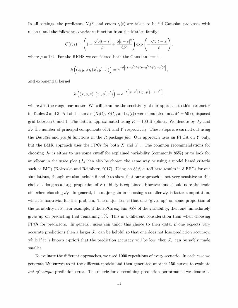
In all settings, the predictors Xi(t) and errors εi(t) are taken to be iid Gaussian processes with

mean 0 and the following covariance function from the Matern family:

C(t, s) =

(1 +

√5|t− s|ρ

+5|t− s|2

3ρ2

)exp

(−√

5|t− s|ρ

),

where ρ = 1/4. For the RKHS we considered both the Gaussian kernel

k(

(x, y, z), (x′, y′, z′))

= e−δ

[(x−x′ )2+(y−y′ )2+(z−z′ )2

],

and exponential kernel

k(

(x, y, z), (x′, y′, z′))

= e−δ

[|x−x′ |+|y−y′ |+|z−z′ |

],

where δ is the range parameter. We will examine the sensitivity of our approach to this parameter

in Tables 2 and 3. All of the curves (Xi(t), Yi(t), and εi(t)) were simulated on a M = 50 equispaced

grid between 0 and 1. The data is approximated using K = 100 B-splines. We denote by JX and

JY the number of principal components of X and Y respectively. These steps are carried out using

the Data2fd and pca.fd functions in the R package fda. Our approach uses an FPCA on Y only,

but the LMR approach uses the FPCs for both X and Y . The common recommendations for

choosing JY is either to use some cutoff for explained variability (commonly 85%) or to look for

an elbow in the scree plot (JX can also be chosen the same way or using a model based criteria

such as BIC) (Kokoszka and Reimherr, 2017). Using an 85% cutoff here results in 3 FPCs for our

simulations, though we also include 6 and 9 to show that our approach is not very sensitive to this

choice as long as a large proportion of variability is explained. However, one should note the trade

offs when choosing JY . In general, the major gain in choosing a smaller JY is faster computation,

which is nontrivial for this problem. The major loss is that one “gives up” on some proportion of

the variability in Y . For example, if the FPCs explain 95% of the variability, then one immediately

gives up on predicting that remaining 5%. This is a different consideration than when choosing

FPCs for predictors. In general, users can tailor this choice to their data; if one expects very

accurate predictions then a larger JY can be helpful so that one does not lose prediction accuracy,

while if it is known a-priori that the prediction accuracy will be low, then JY can be safely made

smaller.

To evaluate the different approaches, we used 1000 repetitions of every scenario. In each case we

generate 150 curves to fit the different models and then generated another 150 curves to evaluate

out-of-sample prediction error. The metric for determining prediction performance we denote as

11

RPE, for relative prediction error. This metric denotes the improvement of the predictions over

just using the mean, and can be thought of as a type of out-of-sample R2. An RPE of 0 implies

that the model shows no improvement over just using the mean, while an RPE of 1 means the

predictions are perfect. More precisely, we first compute the Mean Squared Prediction error as:

MSPE =

n∑i=1

‖Yi − Yi‖2L2 ,

where Yi is a predicted value using one of the three discussed models or simply the mean. The

RPE is then defined as

RPE =MSPEmean −MSPE

MSPEmean,

where MSPEmean denotes the MSPE using a mean only model. Note that even in the mean only

model, all parameters are estimated on the initial 150 curves and prediction is then evaluated on

the second 150. Therefore, it is actually possible to have a numerically negative RPE if an approach

isn’t predicting any better than just using the mean.

The RPEs of LMR and LMF for the three models (a), (b), and (c) are summarized in Table

1. For both models, we took JX = 3, which explained over 85% of the variability of the predictors

and for LMR we took JY = 3 PCs for the outcome as well. The RPEs for our approach with

δ = 2−3, 2−2, 2−1, 1, 2 and JY = 3, 6, 9 are summarized in Tables 2 and 3, which represent the

Gaussian and exponential kernels respectively. An initial look at the tables confirms much of what

one would expect. When the true model is linear, the two linear approaches work best, resulting

in about twice the RPE of AFFR. However, when moving to the two nonlinear models, the AFFR

approach does substantially better. This increased performance is seen for any choice of JY and δ.

Furthermore, the prediction performance seems relatively robust to the choice of JY , δ, and even

the kernel. In the case of JY this is not so surprising as over 90% of the variability of the Yi is

explained by the first three FPCs. In contrast, there is some sensitivity to the choice of δ, but it is

relatively weak given how much we are changing δ in each row. In our application section we set

δ using a type of median, but one could also refit the model with a few different δ and choose the

one with the best prediction performance. Given how consistent the AFFR predictions are, trying

a few δ appears to be satisfactory, and large grid searches can be avoided.

As a final illustration of the efficacy of AFFR, we provide several plots to help visualize the

performance. In Figure 1 we plot several realizations of Yi and their corresponding (out of sample)

predictions using the optimal prediction, E[Y (t)|X], AFFR, and the linear model without reducing

the dimension of the Y . We consider only the Gaussian kernel and take δ = 1/4. For the nonlinear

12

Scenario (a) Scenario (b) Scenario (c)

LMR 0.045 0.030 0.060

LMF 0.045 0.029 0.060

Table 1: Relative prediction errors, RPE, for the two linear models. For both, the number of FPCs

for the predictor is JX = 3. LMR also reduces the dimension of the outcome with JY = 3 FPCs.

Scenario (a) Scenario (b) Scenario (c)

JY = 3 JY = 6 JY = 9 JY = 3 JY = 6 JY = 9 JY = 3 JY = 6 JY = 9

δ = 2−3 0.025 0.026 0.026 0.379 0.379 0.379 0.840 0.840 0.845

δ = 2−2 0.024 0.025 0.025 0.370 0.370 0.370 0.816 0.804 0.815

δ = 2−1 0.023 0.024 0.023 0.360 0.361 0.361 0.847 0.831 0.830

δ = 20 0.022 0.023 0.021 0.346 0.347 0.347 0.83 0.83 0.83

δ = 21 0.020 0.021 0.019 0.328 0.328 0.400 0.808 0.808 0.790

PEV 90.45% 99.12% 99.88% 90.82% 99.10% 99.84% 91.25% 99.22% 99.87%

Table 2: Relative prediction error, RPE, for AFFR using a Gaussian kernel and with different kernel

parameter values, δ. In every case the penalty parameter, λ, is chosen using cross-validation. PEV

indicates the proportion of explained variance of Y for the corresponding number of FPCs, JY .

scenarios (rows 2 and 3), one can clearly see the RPE results reflected in the predictions as AFFR

is much closer to the optimal prediction. In Figure 2 we plot several realizations of g(t, s,Xi(s)),

which are again done out of sample along with the true value of g(t, s,Xi(s)). Plotting in this

way allows us to visualize g using surfaces, where as plotting g(t, s, x) would be challenging since

the domain has three coordinates. As we can see, the estimates are quite close to the true values,

capturing the nonlinear structure quite well.

6 Application to Cumulative Intraday Data

We conclude with an illustration of our approach applied to real data. Cumulative Intra-Day

Returns (CIDR’s) consist of daily stock prices that are normalized to start at zero at the beginning

of each trading day. FDA methods have been useful in analyzing such data (Gabrys et al., 2010;

Kokoszka and Reimherr, 2013; Horvath et al., 2014), given the density at which stock prices can

be observed. Let Pi(tj) denote the price of a stock on day i and time of day tj . The CIDRs are

then defined as

Ri(tj) = 100 [lnPi(tj)− lnPi(t1)] , i = 1, ..., n, j = 1, ...,M.

13

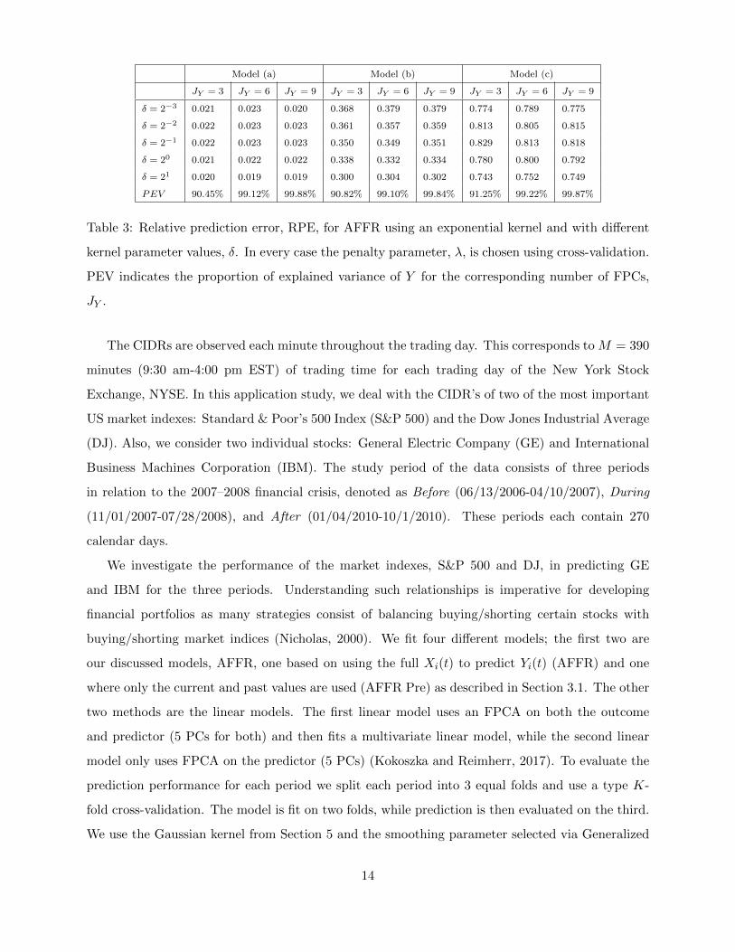
Model (a) Model (b) Model (c)

JY = 3 JY = 6 JY = 9 JY = 3 JY = 6 JY = 9 JY = 3 JY = 6 JY = 9

δ = 2−3 0.021 0.023 0.020 0.368 0.379 0.379 0.774 0.789 0.775

δ = 2−2 0.022 0.023 0.023 0.361 0.357 0.359 0.813 0.805 0.815

δ = 2−1 0.022 0.023 0.023 0.350 0.349 0.351 0.829 0.813 0.818

δ = 20 0.021 0.022 0.022 0.338 0.332 0.334 0.780 0.800 0.792

δ = 21 0.020 0.019 0.019 0.300 0.304 0.302 0.743 0.752 0.749

PEV 90.45% 99.12% 99.88% 90.82% 99.10% 99.84% 91.25% 99.22% 99.87%

Table 3: Relative prediction error, RPE, for AFFR using an exponential kernel and with different

kernel parameter values, δ. In every case the penalty parameter, λ, is chosen using cross-validation.

PEV indicates the proportion of explained variance of Y for the corresponding number of FPCs,

JY .

The CIDRs are observed each minute throughout the trading day. This corresponds to M = 390

minutes (9:30 am-4:00 pm EST) of trading time for each trading day of the New York Stock

Exchange, NYSE. In this application study, we deal with the CIDR’s of two of the most important

US market indexes: Standard & Poor’s 500 Index (S&P 500) and the Dow Jones Industrial Average

(DJ). Also, we consider two individual stocks: General Electric Company (GE) and International

Business Machines Corporation (IBM). The study period of the data consists of three periods

in relation to the 2007–2008 financial crisis, denoted as Before (06/13/2006-04/10/2007), During

(11/01/2007-07/28/2008), and After (01/04/2010-10/1/2010). These periods each contain 270

calendar days.

We investigate the performance of the market indexes, S&P 500 and DJ, in predicting GE

and IBM for the three periods. Understanding such relationships is imperative for developing

financial portfolios as many strategies consist of balancing buying/shorting certain stocks with

buying/shorting market indices (Nicholas, 2000). We fit four different models; the first two are

our discussed models, AFFR, one based on using the full Xi(t) to predict Yi(t) (AFFR) and one

where only the current and past values are used (AFFR Pre) as described in Section 3.1. The other

two methods are the linear models. The first linear model uses an FPCA on both the outcome

and predictor (5 PCs for both) and then fits a multivariate linear model, while the second linear

model only uses FPCA on the predictor (5 PCs) (Kokoszka and Reimherr, 2017). To evaluate the

prediction performance for each period we split each period into 3 equal folds and use a type K-

fold cross-validation. The model is fit on two folds, while prediction is then evaluated on the third.

We use the Gaussian kernel from Section 5 and the smoothing parameter selected via Generalized

14

0.0 0.2 0.4 0.6 0.8 1.0

−0.

4−

0.2

0.0

0.2

0.4

0.6

0.0 0.2 0.4 0.6 0.8 1.0

−0.

4−

0.2

0.0

0.2

0.4

0.6

0.0 0.2 0.4 0.6 0.8 1.0

−0.

4−

0.2

0.0

0.2

0.4

0.6

0.0 0.2 0.4 0.6 0.8 1.0

−0.

4−

0.2

0.0

0.2

0.4

0.6

0.0 0.2 0.4 0.6 0.8 1.0

−1.

5−

1.0

−0.

50.

00.

51.

0

0.0 0.2 0.4 0.6 0.8 1.0

−1.

5−

1.0

−0.

50.

00.

51.

0

0.0 0.2 0.4 0.6 0.8 1.0

−1.

5−

1.0

−0.

50.

00.

51.

0

0.0 0.2 0.4 0.6 0.8 1.0

−1.

5−

1.0

−0.

50.

00.

51.

0

0.0 0.2 0.4 0.6 0.8 1.0

−6

−4

−2

02

0.0 0.2 0.4 0.6 0.8 1.0

−6

−4

−2

02

0.0 0.2 0.4 0.6 0.8 1.0

−6

−4

−2

02

0.0 0.2 0.4 0.6 0.8 1.0

−6

−4

−2

02

Figure 1: Plots of the optimal prediction E[Y (t)|X] (black), prediction using AFFR Y (t) (red

dashed), and prediction using the unreduced linear model YLM (t) (blue dashed). The four plots

on the top row correspond to the scenario (a), which is linear. The four plots in the middle row

correspond to the scenario (b), which is nonlinear. The four plots in the bottom row correspond to

the scenario (c) which is also nonlinear.

Cross-Validation. Prediction performance is then averaged over the 3 folds. To provide a more

readily interpretable metric for prediction performance, we use the same RPE metric given in

Section 5, which denotes the relative performance of a model with respect to a mean only model.

A value of 1 means perfect prediction, while a value of 0 indicates that the model is doing no better

than just using the mean. The results are summarized in Table 4.

As we can see, all models perform better during and after the crisis. This suggests that the

behavior of the market had not returned to its pre-crisis characteristics. Looking at Figure 3, we can

clearly see that the volatility increases during and after the financial crises. This suggests that the

overall “market” effect on the stocks is stronger during periods of high-volatility. When comparing

15

x

y

z

x

y

z

x

y

z

x

y

z

x

y

z

x

y

z

Figure 2: The top row plots one realization of g(t, s,X(s)) for models (a), (b), and (c) respectively.

The bottom row plots the corresponding (out of sample) prediction g(t, s,X(s)).

the four different models, the linear models do nearly the same, which is to be expected since 5

PCs explains over 90% of the variability of the stocks. The AFFR model is not too far behind, but

does noticeably worse in every setting. This suggests that the relationship between the discussed

stocks and the indices is approximately linear; if there are any nonlinear relationships then they

are either very minor deviations from linearity or are not well captured by an additive structure.

The results of AFFR using only current and past values of Xi(t) to predict Yi(t) (AFFR Pre) does

substantially worse before the crises. Interestingly, during and after its performance is closer to

AFFR, though some relationships it still does not capture well. Thus suggests that, unsurprisingly,

knowing the future values of Xi(t) is very helpful for predicting currentvalues of Yi(t), though this

is obviously impractical. During the financial crises, many stocks are likely being driven by large

market level effects. In this setting, AFFR Pre, does quite well, even beating AFFR slightly in

some settings, suggesting that the simpler structure has actually helped with prediction.

16

Period Before During After

Model AFFR AFFR Pre LM Red LM Full AFFR AFFR Pre LM Red LM Full AFFR AFFR Pre LM Red LM Full

GE on DJ 0.133 5.124e-06 0.191 0.191 0.459 0.311 0.536 0.548 0.500 0.421 0.501 0.512

GE on SP 1.325e-07 4.216e-14 0.184 0.183 0.273 0.253 0.458 0.472 0.510 0.436 0.487 0.497

IBM on DJ 0.092 1.645e-03 0.182 0.184 0.274 0.350 0.486 0.495 0.364 0.011 0.402 0.412

IBM on SP 0.079 1.251e-11 0.180 0.180 0.213 0.272 0.373 0.384 0.296 0.009 0.343 0.351

Table 4: Prediction performance of four models: AFFR (our model), AFFR Pre (modifies domain

to avoid using future values), LM Red (linear model with PCA in both the outcome and predictor),

and LM Full (linear model with PCA on the predictor only). The top row corresponds to predicting

GE based on DJ, the second corresponds to prediction GE from SP, and so on. Each number denotes

the relative increase in out-of-sample prediction performance over a mean only model, with 100%

denoting perfect prediction and 0% denoting no increase over just using the mean.

7 Conclusions and Future Work

In this paper we have presented a new RKHS framework for estimating an additive function-

on-function regression model, that is better able to account for complex nonlinear dynamics in

functional regression models than classic linear models. We showed that the estimator is mini-

max in the sense that it achieves an optimal rate of convergence in terms of prediction error. In

addition, computing the estimate is computationally efficient, especially if dimension reduction is

incorporated.

Nonlinear models for functional data have recently received a great deal of attention, however,

there are still a number of interesting questions that remain open. One that is especially relevant

to the work presented here concerns further statistical properties of the estimate, g. In particular,

convergence rates of g as well as its asymptotic distribution would be especially interesting for

quantifying the estimation uncertainty in practice. Using such tools, one could also construct

confidence/prediction bands, which would be of great use in practice.

Another nontrivial extension would be to curves that are observed sparsely. Nonlinear models

in FDA often require that the curves be observed or at least consistently estimated. However, for

some data this is unrealistic and there is a great deal of uncertainty related to imputing the curves.

Lastly, extensions to more complex settings would also be of interest. For example, the handling

of more complex domains, e.g. space or space-time. In these cases, the minimax rates usually

depend on the dimension of the domain. Another important extension would be to functional

binary or categorical outcomes (as opposed to quantitative) would be of interest as one must

17

Figure 3: Plots of the intraday cumulative returns for the Dow Jones Index (top) and General

Electric (bottom) before (left), during (middle), and after (right) the 2008 financial crisis.

incorporate tools from functional glms.

A Proof of Theorem 1

A.1 Excess Risk

We begin by expressing the excess risk in an alternative form. Recall that k(t, s, x; t′, s′, x′) is the

kernel function used to define the RKHS, K. This kernel can be viewed as the kernel of an integral

operator, Lk, which maps L2([0, 1]2 × R)→ K ⊂ L2([0, 1]2 × R). In particular

(Lkf)(t, s, x) =

∫ ∫ ∫k(t, s, x; t′, s′, x′)f(t′, s′, x′) dt′ds′dx′.

From here on, for simplicity, we will denote L2([0, 1]2×R) as simply L2. By Assumption 1, Lk is a

positive definite, compact operator, which is also self-adjoint in the sense that 〈f,Lkg〉 = 〈Lkf, g〉,

for any f and g in L2. We can therefore define a square-root of Lk, denoted as L1/2k that satisfies

f1 ∈ K⇐⇒ L−12

k f1 ∈ L2 and L12k f2 ∈ K⇐⇒ f2 ∈ L2.

Note that if Lk has a nontrivial null space, then L−1/2k can still be well defined since assuming

f ∈ K means that f is orthogonal to the null space of L. Recall that one can also move between

the K and L2 inner product as follows

〈f, g〉K = 〈L−1/2k f,L−1/2

k g〉L2 = 〈f,L−1k g〉L2 .

18

We refer the interested reader to Kennedy and Sadeghi (2013) for more details.

Let g denote our estimate of the true function, g. We then define the following

k12

t,s,X(s) = L−12

k kt,s,X(s), h = L−12

k g and h = L−12

k g.

Using the reproducing property, we have that

g(t, s,X(s)) = 〈k12

t,s,X(s), h〉L2 and g(t, s,X(s)) = 〈k12

t,s,X(s), h〉L2 .

Now define the random operator, T : L2 → L2 as

Tt,s,s′ = k1/2t,s,Xn+1(s) ⊗ k

1/2t,s′,Xn+1(s′),

where ⊗ denotes the tensor product, and the resulting object is interpreted as an operator:

Tt,s,s′(f) = k1/2t,s,Xn+1(s)〈k

1/2t,s′,Xn+1(s′), f〉L2 .

We also define a second operator, which integrates out t, s, and s′, and takes an expectation over

Xn+1:

C = E

[∫ 1

0

∫ 1

0

∫ 1

0Tt,s,s′dsds

′dt

].(5)

Note that C is a symmetric, positive definite, compact operator, and thus has a spectral decompo-

sition

C =∞∑k=1

ρk(φk ⊗ φk),(6)

where ρk ≥ 0 and φk ∈ L2 are, respectively, the eigenvalues and eigenfunctions of C. This decom-

position will be used later on.

As we said before, denote by E∗ the expected value conditioned on the data (X1, Y1), ..., (Xn, Yn).

19

The excess risk can be written as

<n = E∗∫ 1

0

(∫ 1

0[g(t, s,Xn+1(s))− g(t, s,Xn+1(s)))] ds

)2

dt

= E∗∫ 1

0

(∫ 1

0

[〈k

12

t,s,Xn+1(s), hλ〉L2 − 〈k12

t,s,Xn+1(s), h〉L2

]ds

)2

dt

= E∗∫ 1

0

(∫ 1

0〈k

12

t,s,Xn+1(s), hλ − h〉L2ds

)2

dt

= E∗∫ 1

0

∫ 1

0

∫ 1

0〈k

12

t,s,Xn+1(s), h− h〉L2〈k12

t,s′,Xn+1(s′), h− h〉L2dsds′dt

= E∗∫ 1

0

∫ 1

0

∫ 1

0〈Tt,s,s′(h− h), h− h〉L2dsds′dt

= 〈C(h− h), h− h〉L2 = ‖h− h‖2C .

Thus, the excess risk can be expressed as sort of a weighted L2 norm, where the operator C defines

the weights, which is composed of the kernel and the distribution of Xn+1.

A.2 Re-expressing the Estimator

In this section we define an alternative form for the estimator g, which was given in Section 3.

In particular, instead of using the reproducing property, we will write down the estimator using

operators. To do this, we will take derivatives of RSSλ(g) with respect to g. Since these are

functions, we mean the Frechet derivative or strong derivative. Note that RSSλ(g) is a convex

differentiable functional over K. However, so that we are working with L2 instead of K, we use

RSSλ(h) := RSSλ(L1/2k h), where h = L−1/2

k g:

RSSλ(h) =n∑i=1

∫ 1

0

(Yi(t)−

∫ 1

0〈h, k1/2

t,s,Xi(s)〉L2ds

)2

dt+ λ‖h‖2L2 .

Now RSSλ(h) is a convex differentiable functional over L2. Thus, when taking the derivative, we

are using the topology of L2 not K.

To take the derivative of RSSλ(h) we first focus on the penalty, which is easier. We have that

∂

∂h‖h‖2L2 = 2h.

Turning to the first term in RSSλ(h) we first define the empirical quantities

Ti;t,s,s′ = k1/2t,s,Xi(s)

⊗ k1/2t,s′,Xi(s′)

20

and

Cn =1

n

n∑i=1

∫ 1

0

∫ 1

0

∫ 1

0Ti;t,s,s′dsds

′dt.(7)

Now we can apply a chain rule to obtain

∂

∂h

[1

n

n∑i=1

∫ 1

0

(Yi(t)−

∫ 1

0〈h, k1/2

t,s,Xi(s)〉L2ds

)2

dt

]

= − 2

n

n∑i=1

∫ 1

0

∫ 1

0Yi(t)k

12

t,s,Xi(s)dsdt+ 2Cnh.

For notational simplicity, define

Γk1/2,Y =1

n

n∑i=1

∫ 1

0

∫ 1

0Yi(t)k

12

t,s,Xi(s)dsdt.

So, we finally have that∂

∂hRSSλ(h) = −2Γk1/2,Y + 2Cnh+ 2λh,

which yields the estimate

h = (Cn + λI)−1Γk1/2,Y ,(8)

where I is the identity operator.

A.3 Proof of Theorem 1 - Controlling Bias

Using Assumption 1 we can express

Yi(t) =

∫〈k1/2t,s,Xi(s)

, h〉L2 + εi(t).

and we therefore have that

Γk1/2,Y = Cn(h) + fn

where

fn =1

n

n∑i=1

∫ 1

0

∫ 1

0εi(t)k

12

t,s,Xi(s)dsdt.

This implies that h from (8) can be expressed as

h = (Cn + λI)−1Cn(h) + (Cn + λI)−1fn.

We introduce an intermediate quantity, hλ, which is given by

hλ = (C + λI)−1C(h),

21

where C is defined in (5). The difference between hλ and h represents the bias of the estimator h.

Balancing this quantity with the variance, discussed in the next section, is called the bias-variance

trade off a common term in nonparametric smoothing. Inherently, the idea is that to achieve an

optimal h we have to balance both the bias and variance so that neither one is overly large.

Using the eigenfunctions of C as a basis, we can write

h =

∞∑k=1

akφk.

Since C and C + I have the same eigenfunctions, it follows that we can express

C + λI =∞∑k=1

(λ+ ρk)(φk ⊗ φk) =⇒ (C + λI)−1 =∞∑k=1

(λ+ ρk)−1(φk ⊗ φk).

So we have that hλ can be expressed as

hλ = (C + λI)−1C(h) =

∞∑k=1

akρkλ+ ρk

φk.

So the difference, hλ − h can be written as

hλ − h = −∞∑k=1

λakλ+ ρk

φk.(9)

The bias is therefore given by

‖hλ − h‖2C =∞∑k=1

λ2a2kρk

(λ+ ρk)2≤ λ2 max

k≥1

ρk(λ+ ρk)2

∞∑k=1

a2k = λ2‖h‖2L2 max

k≥1

ρk(λ+ ρk)2

.

It is easy to verify that the maximum of F (x) = x/(λ+x)2 is achieved at x = λ with the maximum

value being 14λ . We can therefore bound the bias as

‖hλ − h‖2C ≤λ‖h‖2L2

4.

In the statement of Theorem 1 we assume that λ n2r/(2r+1), which implies that the bias is of the

order n−2r

2r+1O(1). We will show in the next section that the variance of our estimate achieves the

same order.

A.4 Proof of Theorem 1 - Controlling Variability

Controlling the variability of the estimates, ‖h− hλ‖C follows similar arguments as controlling the

bias. However, there are many more terms which must be analyzed separately. In particular, we

decompose h− hλ into five separate components:

h− hλ = T1 + T2 + T3 + T4 + T5,(10)

22

where the Ti terms are given by

T1 = (C + λI)−1C(hλ − h),

T2 = λ(C + λI)−2C(h),

T3 = −(C + λI)−1fn,

T4 = (C + λI)−1(Cn − C)(hλ − h),

T5 = (C + λI)−1(C − Cn)(hλ − h).

While a bit tedious, it only requires linear algebra and repeated calls to the definitions of h and hλ to

verify (10), we thus omit the details here. We now develop bounds for each term, ‖Ti‖C , separately.

For the first four, it turns out to be convenient to bound ‖CνTi‖L2 for 0 < ν ≤ 1/2, as these bounds

will be needed for the final term T5. Notice that when ν = 1/2 we have ‖CνTi‖L2 = ‖Ti‖C .

1. Using the eigenfunctions of C to express hλ − h as in (9), we get that

T1 = −∞∑k=1

λakρk(λ+ ρk)2

φk.

We then have that

‖CνT1‖2L2 =∞∑k=1

λ2a2kρ

2(1+ν)k

(λ+ ρk)4≤ λ2 max

k≥1

ρ2(1+ν)k

(λ+ ρk)4‖h‖2L2 .

Again, it is a basic calculus exercise to show that

maxk≥1

ρ2(1+ν)k

(λ+ ρk)4≤

(λ1+ν

1−ν

)2(1+ν)

(λ+ λ1+ν

1−ν

)4 =(1− ν)2(1−ν)(1 + ν)2(1+ν)

16

1

λ2−2ν.

We thus have the bound

‖CνT1‖2L2 ≤ cλ2ν‖h‖2L2 ,(11)

where c is a constant that depends only on ν.

2. Using the same arguments as in the previous step, we have that

‖CνT2‖2L2 =

∞∑k=1

λ2a2kρ

2(1+ν)k

(λ+ ρk)4≤ λ2 max

k≥1

ρ2(1+ν)k

(λ+ ρk)4

∞∑k=1

a2k ≤ cλ2ν‖h‖2L2 .(12)

3. Turning to T3, we apply Lemma 1 with 0 < ν ≤ 1/2 to obtain

‖CνT3‖2L2 = ‖Cν(C + λI)−1fn‖L2 =1

nλ1−2ν+1/2rOp(1),

23

where r is defined as in Assumption 1. By the statement of Theorem 1 it follows that nλ1+ 12r

tends to a nonzero constant, meaning that

1

nλ1−2ν+ 12r

λ2ν → 0,(13)

since λ→ 0. Thus we have that ‖CνT3‖L2 = Op(λν).

4. To bound T4 we first fix a second value ν > ν2 > 0 that satisfies 2r(1−2ν2) > 1, or equivalently

ν2 < (2r−1)/4r, as well as 4r(2ν2 +2ν) > 1, which is possible as long as r > 1/2 (Assumption

1). We now apply a basic operator inequality

‖CνT4‖L2 = ‖Cν(C + λI)−1(Cn − C)(hλ − h)‖L2

≤ ‖Cν(C + λI)−1(Cn − C)C−ν2‖op‖Cν2(hλ − h)‖L2 .

and then apply Lemmas 3 and 4 to obtain

‖CνT4‖2L2 ≤ Op((

nλ1−2ν+ 12r

)−1)Op(λ2ν2

)=

1

nλ1−2ν+ 12r

op (1) ,(14)

since ν2 > 0 and λ→ 0. Using (13) we conclude that ‖CνT4‖L2 = Op(λν).

5. The last term is the most involved to bound and the reason why the previous four bounds

involved CνTi. We begin by expressing

‖T5‖C = ‖C12 (C + λI)−1(C − Cn)(hλ − h)‖L2

≤ ‖C12 (C + λI)−1(C − Cn)C−ν‖op‖Cν(hλ − h)‖L2 .

Here ν > 0 is chosen to satisfy 2r(1− 2ν) > 1. Applying Lemma 3, we have that

‖T5‖2C ≤1

nλ1/2rOp(1)‖Cν(h− h)‖2L2 .

We have now, in some sense, looped back and are dealing with the term h − h. Using (10)

we have

‖Cν(h− h)‖L2 ≤ ‖CνT1‖L2 + ‖CνT2‖L2 + ‖CνT3‖L2 + ‖CνT4‖L2 + ‖CνT5‖L2 .(15)

The first four terms we already have bounds for, so we need only focus on the last, which

again, has looped back to our original term. We now apply Lemma 2 to obtain

‖CνT5‖2L2 = ‖Cν(C + λI)−1(C − Cn)(h− h)‖2L2 ≤1

nλ1−2ν+ 12r

‖Cν(h− h)‖2L2 .

24

Combining the above with (15) we have that

‖Cν(h− h)‖L2

(1− 1

nλ1−2ν+ 12r

)≤ ‖CνT1‖L2 + ‖CνT2‖L2 + ‖CνT3‖L2 + ‖CνT4‖L2 .

Using (13) it thus follows that

‖Cν(h− h)‖L2 = Op(1)(‖CνT1‖L2 + ‖CνT2‖L2 + ‖CνT3‖L2 + ‖CνT4‖L2),

and applying steps 1-4 we get that

‖Cν(h− h)‖L2 = Op(λν) = op(1),

and we finally have that

‖T5‖C =1

nλ12r

op(1).

We can now combine Steps 1-4, taking ν = 1/2, with step 5 to finally conclude that

<2n = ‖h− h‖2C = λ2Op(1) = n−

2r2r+1Op(1).

Combined with the results of Section A.3, this concludes the proof.

A.5 Auxiliary Lemmas

Here we state four lemmas which are generalizations of ones used in Cai and Yuan (2012) and Wang

and Ruppert (2015).

Lemma 1. If Assumption 1 holds then for any 0 ≤ ν ≤ 12

‖Cν(C + λI)−1fn‖L2 = Op

((nλ1−2ν+ 1

2r

)− 12

).

Lemma 2. Let Assumption 1 hold. Then for any ν > 0 such that 2r(1− 2ν) > 1, we have that

‖Cν(C + λI)−1(Cn − C)C−ν‖op = Op

((nλ1−2ν+ 1

2r

)− 12

),

where ‖.‖op represents the usual operator norm i.e., ‖A‖op = suph:‖h‖L2=1 ‖Ah‖.

Lemma 3. Let Assumption 1 hold and fix 0 < ν < ν2 to be any two values that satisfy 2r(1−2ν) > 1

and 4r(ν2 + ν) > 1, then we have that

‖Cν2(C + λI)−1(Cn − C)C−ν‖op = Op

((nλ1−2ν2+ 1

2r

)− 12

).

25

Lemma 4. (Cai and Yuan, 2012, Lemma 1) For any 0 < ν < 1,

‖Cν(hλ − h)‖L2 ≤ (1− ν)1−νννλν‖h‖L2 .

Lemma 5. Fix ν > 0 and ν2 > 0 such that 4r(ν2 +ν) > 1. If there exist constants 0 < c1 < c2 <∞

such that c1k−2r < sk < c2k

−2r, then there exist constants c3, c4 > 0 depending only on c1, c2 such

that

c4λ−12r−1+2ν2 ≤

∞∑j=1

s2ν2+2νj

(λ+ sj)1+2ν≤ c3(1 + λ

−12r−1+2ν2).

Proof of Lemma 1

Recall that

fn =1

n

n∑i=1

∫ 1

0

∫ 1

0εi(t)k

12

t,s,Xi(s)dsdt.

Using Parseval’s identity we have that

‖Cν(C + λI)−1fn‖2L2 =

∞∑k=1

ρ2νk

(λ+ ρk)2〈fn, φk〉2.

Taking expected values yields

E ‖Cν(C + λI)−1fn‖2L2 =1

n

∞∑k=1

ρ2νk

(λ+ ρk)2E

(∫ 1

0

∫ 1

0ε(t)〈k

12

t,s,X(s), φk〉L2dsdt

)2

.

By Jensen’s inequality we have(∫ 1

0

∫ 1

0ε(t)〈k

12

t,s,X(s), φk〉L2dsdt

)2

≤∫ 1

0

(∫ 1

0ε(t)〈k

12

t,s,X(s), φk〉L2ds

)2

dt

=

∫ 1

0

∫ 1

0

∫ 1

0ε2(t)〈k

12

t,s,X(s), φk〉L2〈k12

t,s∗,X(s∗), φk〉L2dsds∗dt.

Using the assumed independence between ε and X, as well as the assumption that E(ε2(t)) ≤ M ,

where M is a constant, we obtain

E

(∫ 1

0

∫ 1

0ε(t)〈k

12

t,s,X(s), φk〉L2dsdt

)2

≤M E

(∫ 1

0

∫ 1

0

∫ 1

0〈k

12

t,s,X(s), φk〉L2〈k12

t,s∗,X(s∗), φk〉L2dsds∗dt

)= M〈C(φk), φk〉 = Mρk.

Since 0 ≤ ν ≤ 12 and both ρk and λ are positive, we can obtain the bound

E ‖Cν(C + λI)−1fn‖2L2 ≤M

n

∞∑k=1

ρ2ν+1k

(λ+ ρk)2≤ M

nλ1−2ν

∞∑k=1

ρ2ν+1k

(λ+ ρk)1+2ν.

Now we apply Lemma 5 with ν2 = 1/2 to obtain

E ‖Cν(C + λI)−1fn‖2L2 ≤c∗

nλ1−2ν+ 12r

,

where c∗ is a constant. An application of Markov’s inequality completes the proof.

26

Proof of Lemma 2

By definition

‖Cν(C + λI)−1(Cn − C)C−ν‖2op = supf :‖f‖L2=1

‖Cν(C + λI)−1(Cn − C)C−νf‖2L2 .

Fix f ∈ L2 such that ‖f‖L2 = 1. We can expand f as

f =∞∑k=1

fkφk,

By Parseval’s identity we have

‖Cν(C + λI)−1(Cn − C)C−νf‖2 =

∞∑j=1

[ρνj

ρj + λ

∞∑k=1

fkρ−νk 〈(Cn − C)φk, φj〉L2

]2

.

Applying the Cauchy-Schwartz inequality and using the fact that ‖f‖L2 = 1 we have that

∞∑k=1

fkρ−νk 〈(Cn − C)φk, φj〉L2 ≤

( ∞∑k=1

ρ−2νk 〈(Cn − C)φk, φj〉2L2

)1/2

.

So we can bound the operator norm as

‖Cν(C + λI)−1(Cn − C)C−ν‖2op ≤∞∑k=1

∞∑j=1

ρ−2νk ρ2ν

j

(λ+ ρj)2〈φj , (Cn − C)φk〉2L2 .

Applying Jensen’s equality we get that

E

∞∑k=1

∞∑j=1

ρ−2νk ρ2ν

j

(λ+ ρj)2〈φj , (Cn − C)φk〉2L2

12

≤

∞∑k=1

∞∑j=1

ρ−2νk ρ2ν

j

(λ+ ρj)2E〈φj , (Cn − C)φk〉2L2

12

.

Using the definition of Cn from (7) we have that

E〈φj , (Cn − C)φk〉2L2≤E〈φj , Cnφk〉2L2 =1

nE

(∫ 1

0

∫ 1

0

∫ 1

0〈k

12

t,s,X(s), φj〉〈k12

t,s∗,X(s∗), φk〉dsds∗dt

)2

.

Note the first inequality follows from the fact that C is the mean of Cn and thus replacing C above

with any other quantity cannot decrease it (since it is minimized when using C). One can show

this using basic calculus arguments over Hilbert spaces, thus we omit the details here. By applying

Cauchy-Schwartz inequality and Fubini’s theorem we have

E〈φj , (Cn − C)φk〉2L2

≤ 1

nE

([∫ 1

0

(∫ 1

0〈k

12

t,s,X(s), φj〉ds)2

dt

][∫ 1

0

(∫ 1

0〈k

12

t∗,s∗,X(s∗), φk〉ds∗)2

dt∗

])

=1

n

∫ 1

0

∫ 1

0E

[(∫ 1

0〈k

12

t,s,X(s), φj〉ds)2(∫ 1

0〈k

12

t∗,s∗,X(s∗), φk〉ds∗)2]dtdt∗.

27

Using Cauchy-Schwartz inequality again

E〈φj , (Cn − C)φk〉2L2

≤ 1

n

∫ 1

0

∫ 1

0E

12

(∫ 1

0〈k

12

t,s,X(s), φj〉ds)4

E12

(∫ 1

0〈k

12

t∗,s∗,X(s∗), φk〉ds∗)4

dtdt∗.

Note that we can move to the K inner product to obtain:

〈k12

t,s,X(s), φk〉L2 = 〈kt,s,X(s),L1/2k φk〉K = (L1/2

k φk)(t, s,X(s))

and L1/2φk is a function in K, thus we can apply Assumption 1.4 to obtain

E〈φj , (Cn − C)φk〉2L2 ≤c

nE

[∫ 1

0

(∫ 1

0〈k

12

t,s,X(s), φj〉ds)2

dt

]E

[∫ 1

0

(∫ 1

0〈k

12

t∗,s∗,X(s∗), φk〉ds∗)2

dt∗

].

It is easy to see that

E

[∫ 1

0

(∫ 1

0〈k

12

t,s,X(s), φj〉ds)2

dt

]= ρj .

Now we obtain

E〈φj , (Cn − C)φk〉2L2 ≤ cn−1ρjρk.

Therefore,

E

∞∑k=1

∞∑j=1

ρ−2νk ρ2ν

j

(λ+ ρj)2〈φj , (Cn − C)φk〉L2

12

≤

c

n

∞∑k=1

∞∑j=1

ρ1−2νk ρ1+2ν

j

(λ+ ρj)2

12

.

Note that

∞∑k=1

∞∑j=1

ρ1−2νk ρ1+2ν

j

(λ+ ρj)2=∞∑k=1

ρ1−2νk

∞∑j=1

ρ1+2νj

(λ+ ρj)2.

Since 2r(1− 2ν) > 1 and ρk < c2k−2r we have

∞∑k=1

ρ1−2νk ≤ c2

∞∑k=1

k−2r(1−2ν) = c∗∗ <∞.

Finally, by applying Lemma 5 with ν2 = 1/2 we obtain

E ‖Cν(C + λI)−1(Cn − C)C−ν‖op ≤ γ(nλ1−2ν+ 12r )−

12 ,

An application of Markov’s inequality completes the proof.

28

Proof of Lemma 3

Recall that

‖Cν2(C + λI)−1(Cn − C)C−ν‖2op = suph:‖h‖L2=1

‖Cν2(C + λI)−1(Cn − C)C−νh‖2L2 .

Note that

Cν2(C + λI)−1 =

∞∑j=1

ρν2jρj + λ

(φj ⊗ φj),

and recall that from the proof of Lemma 2,

(Cn − C)C−νh =

∞∑k=1

akρ−νk (Cn − C)φk.

Therefore

Cν2(C + λI)−1(Cn − C)C−νh =∞∑j=1

ρν2jρj + λ

〈∞∑k=1

akρ−νk (Cn − C)φk, φj〉L2φj .

By Parseval’s identity we obtain

‖Cν2(C + λI)−1(Cn − C)C−ν‖2op =

∞∑j=1

[ρν2j

ρj + λ〈∞∑k=1

akρ−νk (Cn − C)φk, φj〉L2

]2

By Cauchy-Schwartz inequality and using the same steps in the proof of Lemma 2, we have

‖Cν2(C + λI)−1(Cn − C)C−ν‖2op ≤∞∑k=1

∞∑j=1

ρ−2νk ρ2ν2

j

(λ+ ρj)2〈φj , (Cn − C)φk〉2L2 .

Using the same arguments in the proof of Lemma 2, we obtain

E

∞∑k=1

∞∑j=1

ρ−2νk ρ2ν2

j

(λ+ ρj)2〈φj , (Cn − C)φk〉L2

12

≤

c

n

∞∑k=1

∞∑j=1

ρ1−2νk ρ1+2ν2

j

(λ+ ρj)2

12

.

Note that

∞∑k=1

∞∑j=1

ρ1−2νk ρ1+2ν2

j

(λ+ ρj)2=∞∑k=1

ρ1−2νk

∞∑j=1

ρ1+2ν2j

(λ+ ρj)2.

Note that the condition 2r(1− 2ν) > 1 implies ν < 12 −

12r <

12 . We therefore have(

λ+ ρjρj

)2ν−1

≤ 1.

It follows that

∞∑k=1

∞∑j=1

ρ1−2νk ρ1+2ν2

j

(λ+ ρj)2≤∞∑k=1

ρ1−2νk

∞∑j=1

ρ2ν+2ν2j

(λ+ ρj)2ν+1.

29

Recall that

∞∑k=1

ρ1−2νk ≤ c2

∞∑k=1

k−2r(1−2ν) = c∗∗ <∞.

Therefore

E ‖Cν2(C + λI)−1(Cn − C)C−ν‖op ≤

cc∗∗n

∞∑j=1

ρ2ν+2ν2j

(λ+ ρj)2ν+1

12

.

By applying Lemma 5 we have that

E ‖C12 (C + λI)−1(Cn − C)C−ν‖op ≤ β(nλ

12r

+1−2ν2)−12 ,

where β is a constant. An application of the Markov inequality completes the proof.

A.6 Proof of Lemma 5

Using the same arguments as in Cai and Yuan (2012), we get that

∞∑j=1

s2ν2+2νj

(λ+ sj)1+2ν=∞∑j=1

s1+2νj

(λ+ sj)1+2νs2ν2−1j

≤∞∑j=1

c1+2ν1 k−2r(1+2ν)

(λ+ c2k−2r)1+2νk−2r(2ν2−1)

= c1+2ν1

∞∑j=1

k−2r(2ν2−1)

(λk2r + c2)1+2ν

≤ c1+2ν1

(1

c2+

∫ ∞1

x−2r(2ν2−1)

(λx2r + c2)1+2νdx

)

= c1+2ν1

(1

c2+ λ2ν2−1−1/2r

∫ ∞λ1/2r

y−2r(2ν2−1)

(y2r + c2)1+2νdy

).

For the integral to be finite, it is enough if 2r(2ν2 + 2ν) ≥ 1 + δ, for some δ > 0, as the integrand

will go to zero faster than y−(1+δ). The argument for the lower bound follows the same arguments.

30

References

A. Berlinet and C. Thomas-Agnan. Reproducing Kernel Hilbert spaces in Probability and Statistics.

Springer Science & Business Media, 2011.

T. T. Cai and M. Yuan. Optimal estimation of the mean function based on discretely sampled

functional data: Phase transition. The Annals of Statistics, 39(5):2330–2355, 2011.

T. T. Cai and M. Yuan. Minimax and adaptive prediction for functional linear regression. Journal

of the American Statistical Association, 107(499):1201–1216, 2012.

P. Du and X. Wang. Penalized likelihood functional regression. Statistica Sinica, pages 1017–1041,

2014.

Y. Fan, G. M. James, and P. Radchenko. Functional additive regression. The Annals of Statistics,

43(5):2296–2325, 2015.

R. Gabrys, L. Horvath, and P. Kokoszka. Tests for error correlation in the functional linear model.

Journal of the American Statistical Association, 105(491):1113–1125, 2010.

T. Hastie and R. Tibshirani. Generalized Additive Models. Wiley Online Library, 1990.

L. Horvath and P. Kokoszka. Inference for Functional Data with Applications, volume 200. Springer,

2012.

L. Horvath, P. Kokoszka, and G. Rice. Testing stationarity of functional time series. Journal of

Econometrics, 179(1):66–82, 2014.

G. M. James and B. W. Silverman. Functional adaptive model estimation. Journal of the American

Statistical Association, 100(470):565–576, 2005.

H. Kadri, E. Duflos, P. Preux, S. Canu, and M. Davy. Nonlinear functional regression: A functional

RKHS approach. In Y. W. Teh and M. Titterington, editors, Proceedings of the Thirteenth

International Conference on Artificial Intelligence and Statistics, volume 9 of Proceedings of

Machine Learning Research, pages 374–380, 2010.

R. A. Kennedy and P. Sadeghi. Hilbert Space Methods in Signal Processing. Cambridge University

Press, 2013.

31

J. S. Kim, A.-M. Staicu, A. Maity, R. J. Carroll, and D. Ruppert. Additive function-on-function

regression. Journal of Computational and Graphical Statistics, 27:234–244, 2018.

G. S. Kimeldorf and G. Wahba. Some results on Tchebycheffian spline functions. Journal of

Mathematical Analysis and Applications, 33:82–95, 1971.

P. Kokoszka and M. Reimherr. Predictability of shapes of intraday price curves. The Econometrics

Journal, 16(3):285–308, 2013.

P. Kokoszka and M. Reimherr. Introduction to Functional Data Analysis. CRC Press, 2017.

Y. Li, T. Hsing, et al. Uniform convergence rates for nonparametric regression and principal

component analysis in functional/longitudinal data. The Annals of Statistics, 38(6):3321–3351,

2010.

H. Lian. Nonlinear functional models for functional responses in reproducing kernel Hilbert spaces.

Canadian Journal of Statistics, 35(4):597–606, 2007.

H. Ma and Z. Zhu. Continuously dynamic additive models for functional data. Journal of Multi-

variate Analysis, 150:1–13, 2016.

M. W. McLean, G. Hooker, A.-M. Staicu, F. Scheipl, and D. Ruppert. Functional generalized

additive models. Journal of Computational and Graphical Statistics, 23(1):249–269, 2014.

J. S. Morris. Functional regression. Annual Review of Statistics and Its Application, 2:321–359,

2015.

H.-G. Muller, Y. Wu, and F. Yao. Continuously additive models for nonlinear functional regression.

Biometrika, pages 607–622, 2013.

J. G. Nicholas. Market Neutral Investing. Bloomberg Press Princeton, NJ, 2000.

A. Parodi and M. Reimherr. FLAME: Simultaneous variable selection and smoothing for function-

on-scalar regression. Technical report, Pennsylvania State University, 2017.

J. Petrovich, M. Reimherr, and C. Daymont. Functional regression models with highly irregular

designs. Technical report, Pennsylvania State University, 2018. (https://arxiv.org/abs/1805.

08518).

32

C. Preda. Regression models for functional data by reproducing kernel Hilbert spaces methods.

Journal of Statistical Planning and Inference, 137(3):829–840, 2007.

J. O. Ramsay and B. Silverman. Functional Data Analysis. Wiley Online Library, 2006.

J. O. Ramsay, G. Hooker, and S. Graves. Functional Data Analysis with R and MATLAB. Springer

Science & Business Media, 2009.

F. Scheipl, A.-M. Staicu, and S. Greven. Functional additive mixed models. Journal of Computa-

tional and Graphical Statistics, 24(2):477–501, 2015.

X. Sun, P. Du, X. Wang, and P. Ma. Optimal penalized function-on-function regression under a

reproducing kernel Hilbert space framework. Journal of the American Statistical Association,

page Accepted, 2017.

K. G. van den Boogaart. tensorA: Advanced tensors arithmetic with named indices. R package

version 0.31, 2007. http://CRAN.R-project.org/package=tensorA.

X. Wang and D. Ruppert. Optimal prediction in an additive functional model. Statistica Sinica,

25:567–589, 2015.

L. Xiao, C. Li, W. Checkley, and C. Crainiceanu. Fast covariance estimation for sparse functional

data. Statistics and Computing, pages 1–12, 2017.

F. Yao, H.-G. Muller, and J.-L. Wang. Functional data analysis for sparse longitudinal data.

Journal of the American Statistical Association, 100(470):577–590, 2005.

X. Zhang, J.-L. Wang, et al. From sparse to dense functional data and beyond. The Annals of

Statistics, 44(5):2281–2321, 2016.

H. Zhu, F. Yao, and H. H. Zhang. Structured functional additive regression in reproducing kernel

Hilbert spaces. Journal of the Royal Statistical Society: Series B (Statistical Methodology), 76

(3):581–603, 2014.

33