Embed Size (px)
Citation preview

Matrix differential calculus
10-725 OptimizationGeoff Gordon
Ryan Tibshirani

Geoff Gordon—10-725 Optimization—Fall 2012
Review
• Matrix differentials: sol’n to matrix calculus pain‣ compact way of writing Taylor expansions, or …
‣ definition:
‣ df = a(x; dx) [+ r(dx)]
‣ a(x; .) linear in 2nd arg
‣ r(dx)/||dx|| → 0 as dx → 0
• d(…) is linear: passes thru +, scalar *
• Generalizes Jacobian, Hessian, gradient, velocity
2

Geoff Gordon—10-725 Optimization—Fall 2012
Review
• Chain rule
• Product rule
• Bilinear functions: cross product, Kronecker, Frobenius, Hadamard, Khatri-Rao, …
• Identities
‣ rules for working with , tr()
‣ trace rotation
• Identification theorems
3

Geoff Gordon—10-725 Optimization—Fall 2012
Finding a maximumor minimum, or saddle point
43 2 1 0 1 2 31
0.5
0
0.5
1
1.5
2
ID for df(x) scalar x vector x matrix X
scalar f
vector f
matrix F
df = a dx df = aTdx df = tr(ATdX)
df = a dx df = A dx
dF = A dx

Geoff Gordon—10-725 Optimization—Fall 2012
Finding a maximumor minimum, or saddle point
5
ID for df(x) scalar x vector x matrix X
scalar f
vector f
matrix F
df = a dx df = aTdx df = tr(ATdX)
df = a dx df = A dx
dF = A dx

Geoff Gordon—10-725 Optimization—Fall 2012
And so forth…
• Can’t draw it for X a matrix, tensor, …
• But same principle holds: set coefficient of dX to 0 to find min, max, or saddle point:‣ if df = c(A; dX) [+ r(dX)] then
‣ so: max/min/sp iff
‣ for c(.; .) any “product”,
6

Geoff Gordon—10-725 Optimization—Fall 2012
Ex: Infomax ICA
• Training examples xi ∈ ℝd, i = 1:n
• Transformation yi = g(Wxi)
‣W ∈ ℝd!d
‣ g(z) =
• Want:
23
10 5 0 5 1010
5
0
5
10
Wxi
0.2 0.4 0.6 0.8
0.2
0.4
0.6
0.8
yi
10 5 0 5 1010
5
0
5
10
xi

Geoff Gordon—10-725 Optimization—Fall 2012
Volume rule
8

Geoff Gordon—10-725 Optimization—Fall 2012
Ex: Infomax ICA• yi = g(Wxi)‣ dyi =
• Method: maxW !i –ln(P(yi))‣ where P(yi) =
24
10 5 0 5 1010
5
0
5
10
Wxi
0.2 0.4 0.6 0.8
0.2
0.4
0.6
0.8
yi
10 5 0 5 1010
5
0
5
10
xi

Geoff Gordon—10-725 Optimization—Fall 2012
Gradient
• L = ! ln |det Ji| yi = g(Wxi) dyi = Ji dxi
10
i

Geoff Gordon—10-725 Optimization—Fall 2012
Gradient
11
Ji = diag(ui) W dJi = diag(ui) dW + diag(vi) diag(dW xi) W
dL =

Geoff Gordon—10-725 Optimization—Fall 2012
Natural gradient
• L(W): Rd"d → R dL = tr(GTdW)
• step S = arg maxS M(S) = tr(GTS) – ||SW-1||2 /2‣ scalar case: M = gs – s2 / 2w2
• M =
• dM =
12
F

Geoff Gordon—10-725 Optimization—Fall 2012
yi
ICA natural gradient
• [W-T + C] WTW =
13
Wxi
start with W0 = I

Geoff Gordon—10-725 Optimization—Fall 2012
yi
ICA natural gradient
• [W-T + C] WTW =
13
Wxi
start with W0 = I

Geoff Gordon—10-725 Optimization—Fall 2012
ICA on natural image patches
14

Geoff Gordon—10-725 Optimization—Fall 2012
ICA on natural image patches
15

Geoff Gordon—10-725 Optimization—Fall 2012
More info• Minka’s cheat sheet:‣ http://research.microsoft.com/en-us/um/people/minka/
papers/matrix/
• Magnus & Neudecker. Matrix Differential Calculus. Wiley, 1999. 2nd ed.‣ http://www.amazon.com/Differential-Calculus-
Applications-Statistics-Econometrics/dp/047198633X
• Bell & Sejnowski. An information-maximization approach to blind separation and blind deconvolution. Neural Computation, v7, 1995.
16

Newton’s method
10-725 OptimizationGeoff Gordon
Ryan Tibshirani

Geoff Gordon—10-725 Optimization—Fall 2012
Nonlinear equations
• x ∈ Rd f: Rd→Rd, diff ’ble
‣ solve:
• Taylor:‣ J:
• Newton:
18
0 1 21
0.5
0
0.5
1
1.5

Geoff Gordon—10-725 Optimization—Fall 2012
Error analysis
19

Geoff Gordon—10-725 Optimization—Fall 2012
dx = x*(1-x*phi)
20
0: 0.7500000000000000 1: 0.58985588132818412: 0.61674926047875973: 0.61803131814154534: 0.61803398873835475: 0.61803398874989486: 0.61803398874989497: 0.61803398874989488: 0.6180339887498949
*: 0.6180339887498948

Geoff Gordon—10-725 Optimization—Fall 2012
Bad initialization
21
1.3000000000000000-0.1344774409873226-0.2982157033270080-0.7403273854022190-2.3674743431148597
-13.8039236412225819-335.9214859516196157
-183256.0483360671496484-54338444778.1145248413085938

Geoff Gordon—10-725 Optimization—Fall 2012
Minimization
• x ∈ Rd f: Rd→R, twice diff ’ble
‣ find:
• Newton:
22

Geoff Gordon—10-725 Optimization—Fall 2012
Descent
• Newton step: d = –(f ’’(x))-1 f ’(x)
• Gradient step: –g = –f’(x)
• Taylor: df =
• Let t > 0, set dx = ‣ df =
• So:
23
Geoff Gordon—10-725 Optimization—Fall 2012
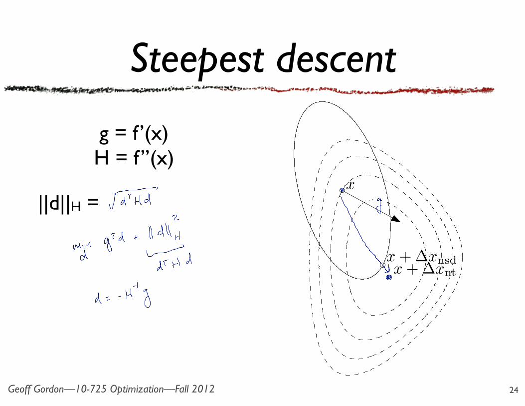
Steepest descent
24
9.5 Newton’s method 485
PSfrag replacements
x
x + !xntx + !xnsd
Figure 9.17 The dashed lines are level curves of a convex function. Theellipsoid shown (with solid line) is {x + v | vT!2f(x)v " 1}. The arrowshows #!f(x), the gradient descent direction. The Newton step !xnt isthe steepest descent direction in the norm $ · $!2f(x). The figure also shows!xnsd, the normalized steepest descent direction for the same norm.
Steepest descent direction in Hessian norm
The Newton step is also the steepest descent direction at x, for the quadratic normdefined by the Hessian !2f(x), i.e.,
"u"!2f(x) = (uT!2f(x)u)1/2.
This gives another insight into why the Newton step should be a good searchdirection, and a very good search direction when x is near x!.
Recall from our discussion above that steepest descent, with quadratic norm" · "P , converges very rapidly when the Hessian, after the associated change ofcoordinates, has small condition number. In particular, near x!, a very good choiceis P = !2f(x!). When x is near x!, we have !2f(x) # !2f(x!), which explainswhy the Newton step is a very good choice of search direction. This is illustratedin figure 9.17.
Solution of linearized optimality condition
If we linearize the optimality condition !f(x!) = 0 near x we obtain
!f(x + v) # !f(x) + !2f(x)v = 0,
which is a linear equation in v, with solution v = !xnt. So the Newton step !xnt iswhat must be added to x so that the linearized optimality condition holds. Again,this suggests that when x is near x! (so the optimality conditions almost hold),the update x + !xnt should be a very good approximation of x!.
When n = 1, i.e., f : R $ R, this interpretation is particularly simple. Thesolution x! of the minimization problem is characterized by f "(x!) = 0, i.e., it is
g = f ’(x)H = f’’(x)
||d||H =

Geoff Gordon—10-725 Optimization—Fall 2012
Newton w/ line search
• Pick x1
• For k = 1, 2, …‣ gk = f ’(xk); Hk = f ’’(xk)
‣ dk = –Hk \ gk
‣ tk = 1
‣ while f(xk + tk dk) > f(xk) + t gkTdk / 2
‣ tk = β tk
‣ xk+1 = xk + tk dk
25
gradient & Hessian
Newton direction
backtracking line search
step
β<1

Geoff Gordon—10-725 Optimization—Fall 2012
Properties of damped Newton
• Affine invariant: suppose g(x) = f(Ax+b)‣ x1, x2, … from Newton on g()
‣ y1, y2, … from Newton on f()
‣ If y1 = Ax1 + b, then:
• Convergent: ‣ if f bounded below, f(xk) converges
‣ if f strictly convex, bounded level sets, xk converges
‣ typically quadratic rate in neighborhood of x*
26