Matrix Completion and Low-Rank SVD via Fast Alternating

Journal of Machine Learning Research 16 (2015) 3367-3402 Submitted 10/14; Revised 2/15; Published 12/15

Matrix Completion and Low-Rank SVD via Fast AlternatingLeast Squares

Trevor Hastie [email protected] of StatisticsStanford University, CA 94305, USA

Rahul Mazumder [email protected] of StatisticsColumbia UniversityNew York, NY 10027, USA

Jason D. Lee [email protected] for Computational and Mathematical EngineeringStanford University, CA 94305, USA

Reza Zadeh [email protected]

Databricks

2030 Addison Street, Suite 610

Berkeley, CA 94704, USA

Editor: Guy Lebanon

Abstract

The matrix-completion problem has attracted a lot of attention, largely as a result ofthe celebrated Netflix competition. Two popular approaches for solving the problem arenuclear-norm-regularized matrix approximation (Candes and Tao, 2009; Mazumder et al.,2010), and maximum-margin matrix factorization (Srebro et al., 2005). These two proce-dures are in some cases solving equivalent problems, but with quite different algorithms. Inthis article we bring the two approaches together, leading to an efficient algorithm for largematrix factorization and completion that outperforms both of these. We develop a softwarepackage softImpute in R for implementing our approaches, and a distributed version forvery large matrices using the Spark cluster programming environment

Keywords: matrix completion, alternating least squares, svd, nuclear norm

1. Introduction

We have an m × n matrix X with observed entries indexed by the set Ω; i.e. Ω = (i, j) :Xij is observed. Following Candes and Tao (2009) we define the projection PΩ(X) to be them× n matrix with the observed elements of X preserved, and the missing entries replacedwith 0. Likewise P⊥Ω projects onto the complement of the set Ω.

Inspired by Candes and Tao (2009), Mazumder et al. (2010) posed the following convex-optimization problem for completing X:

minimizeM

H(M) := 12‖PΩ(X −M)‖2F + λ‖M‖∗, (1)

c©2015 Trevor Hastie and Rahul Mazumder and Jason Lee and Reza Zadeh.

Hastie, Mazumder, Lee and Zadeh

where the nuclear norm ‖M‖∗ is the sum of the singular values of M (a convex relaxationof the rank). They developed a simple iterative algorithm for solving Problem (1), with thefollowing two steps iterated till convergence:

1. Replace the missing entries in X with the corresponding entries from the currentestimate M :

X ← PΩ(X) + P⊥Ω (M); (2)

2. Update M by computing the soft-thresholded SVD of X:

X = UDV T (3)

M ← USλ(D)V T , (4)

where the soft-thresholding operator Sλ operates element-wise on the diagonal matrixD, and replaces Dii with (Dii−λ)+. With large λ many of the diagonal elements willbe set to zero, leading to a low-rank solution for Problem (1).

For large matrices, step (3) could be a problematic bottleneck, since we need to computethe SVD of the filled matrix X. In fact, for the Netflix problem (m,n) ≈ (400K, 20K),which requires storage of 8 × 109 floating-point numbers (32Gb in single precision), whichin itself could pose a problem. However, since only about 1% of the entries are observed(for the Netflix dataset), sparse-matrix representations can be used.

Mazumder et al. (2010) use two tricks to avoid these computational nightmares:

1. Anticipating a low-rank solution, they compute a reduced-rank SVD in step (3); if thesmallest of the computed singular values is less than λ, this gives the desired solution.A reduced-rank SVD can be computed by using an iterative Lanczos-style method asimplemented in PROPACK (Larsen, 2004), or by other alternating-subspace meth-ods (Golub and Van Loan, 2012).

2. They rewrite X in (2) as

X =[PΩ(X)− PΩ(M)

]+ M ; (5)

The first piece is as sparse as X, and hence inexpensive to store and compute. Thesecond piece is low rank, and also inexpensive to store. Furthermore, the iterativemethods mentioned in step (1) require left and right multiplications of X by skinnymatrices, which can exploit this special structure.

This softImpute algorithm works very well, and although an SVD needs to be computedeach time step (3) is evaluated, this step can use the previous solution as a warm start. Asone gets closer to the solution, the warm starts tend to be better, and so the final iterationstend to be faster.

Mazumder et al. (2010) also considered a path of such solutions, with decreasing valuesof λ. As λ decreases, the rank of the solutions tend to increase, and at each λ`, the iterativealgorithms can use the solution Xλ`−1

(with λ`−1 > λ`) as warm starts, padded with someadditional dimensions.

3368

Matrix Completion by Fast ALS

Rennie and Srebro (2005) consider a different approach. They impose a rank constraint,and consider the problem

minimizeA,B

F (A,B) :=1

2‖PΩ(X −ABT )‖2F +

λ

2

(‖A‖2F + ‖B‖2F

), (6)

where A is m × r and B is n × r. This so-called maximum-margin matrix factorization(MMMF) criterion1 is not convex in A and B, but it is bi-convex — for fixed B the functionF (A,B) is convex in A, and for fixed A the function F (A,B) is convex in B. Alternatingminimization algorithms (ALS) are often used to minimize Problem (6). Consider A fixed,and we wish to solve Problem (6) for B. It is easy to see that this problem decouples inton separate ridge regressions, with each column Xj of X as a response, and the r-columnsof A as predictors. Since some of the elements of Xj are missing, and hence ignored, thecorresponding rows of A are deleted for the jth regression. So these are really separate ridgeregressions, in that the regression matrices are all different (even though they all derive fromA). By symmetry, with B fixed, solving for A amounts to m separate ridge regressions.

There is a remarkable fact that ties the solutions to Problems (6) and (1) (Mazumderet al., 2010, for example). If the solution to Problem (1) has rank q ≤ r, then it provides asolution to Problem (6). That solution is

A = UrSλ(Dr)12

B = VrSλ(Dr)12 ,

(7)

where Ur, for example, represents the sub-matrix formed by the first r columns of U , andlikewise Dr is the top r× r diagonal block of D. Note that for any solution to Problem (6),multiplying A and B on the right by an orthonormal r × r matrix R would be an equiv-alent solution. Likewise, any solution to Problem (6) with rank r ≥ q gives a solution toProblem (1).

In this paper we propose a new algorithm that profitably draws on ideas used both insoftImpute and MMMF. Consider the two steps (3) and (4). We can alternatively solve theoptimization problem

minimizeA,B

1

2‖X −ABT ‖2F +

λ

2(‖A‖2F + ‖B‖2B), (8)

and as long as we use enough columns in A and B, we will have M = ABT . There areseveral important advantages to this approach:

1. Since X is fully observed, the (ridge) regression operator is the same for each column,and so is computed just once. This reduces the computation of an update of A or Bover ALS by a factor of r.

2. By orthogonalizing the r-column matrices A or B at each iteration, the regressionsare simply matrix multiplies, very similar to those used in the alternating subspacealgorithms for computing the SVD.

1. Actually MMMF also refers to the margin-based loss function that they used, but we will nevertheless usethis acronym.

3369


3. This quadratic regularization amounts to shrinking the higher-order components morethan the lower-order components, and this tends to offer a convergence advantage overthe previous approach (compute the SVD, then soft-threshold).

4. Just like before, these operations can make use of the sparse plus low-rank propertyof X.

As an important additional modification, we replace X at each step using the mostrecently computed A or B. All combined, this hybrid algorithm tends to be faster thaneither approach on their own; see the simulation results in Section 6.1

For the remainder of the paper, we present this softImpute-ALS algorithm in moredetail, and show that it convergences to the solution to Problem (1) for r sufficiently large.We demonstrate its superior performance on simulated and real examples, including theNetflix data. We briefly highlight two publicly available software implementations, anddescribe a simple approach to centering and scaling of both the rows and columns of the(incomplete) matrix.

2. Rank-restricted Soft SVD

In this section we consider a complete matrix X, and develop a new algorithm for findinga rank-restricted SVD. In the next section we will adapt this approach to the matrix-completion problem. We first give two theorems that are likely known to experts; theproofs are very short, so we provide them here for convenience.

Theorem 1 Let Xm×n be a matrix (fully observed), and let 0 < r ≤ min(m,n). Considerthe optimization problem

minimizeZ: rank(Z)≤r

Fλ(Z) := 12 ||X − Z||

2F + λ||Z||∗. (9)

A solution is given by

Z = UrSλ(Dr)VTr , (10)

where the rank-r SVD of X is UrDrVTr and Sλ(Dr) = diag[(σ1 − λ)+, . . . , (σr − λ)+].

Proof We will show that, for any Z the following inequality holds:

Fλ(Z) ≥ fλ(σ(Z)) := 12 ||σ(X)− σ(Z)||22 + λ

∑i

σi(Z), (11)

where, fλ(σ(Z)) is a function of the singular values of Z and σ(X) denotes the vector ofsingular values of X, such that σi(X) ≥ σi+1(X) for all i = 1, . . . ,minm,n.

To show inequality (11) it suffices to show that:

12 ||X − Z||

2F ≥ 1

2 ||σ(X)− σ(Z)||22,

which follows as an immediate consequence of the well-known Von-Neumann trace inequality(Mirsky, 1975; Stewart and Sun, 1990):

Tr(XTZ) := 〈X,Z〉 ≤minm,n∑

i=1

σi(X)σi(Y ),

3370


that provides an upper bound to the trace of the product of two matrices in terms of theinner product of their singular values.

Observing that

rank(Z) ≤ r ⇐⇒ ‖σ(Z)‖0 ≤ r,

we have established:

minZ: rank(Z)≤r

(12 ||X − Z||

2F + λ||Z||∗

)≥ min

σ(Z):‖σ(Z)‖0≤r

(12 ||σ(X)− σ(Z)||22 + λ

∑i

σi(Z)

)(12)

Observe that the optimization problem in the right hand side of (12) is a separable vectoroptimization problem. We claim that the optimum solutions of the two problems appearingin (12) are in fact equal. To see this, let

σ(Z) = arg minσ(Z):‖σ(Z)‖0≤r

(12 ||σ(X)− σ(Z)||22 + λ

∑i

σi(Z)

).

If the SVD of X is given by UDV T , then the choice Z = Udiag(σ(Z))V T satisfies

rank(Z) ≤ r and Fλ(Z) = fλ(σ(Z))

This shows that:

minZ: rank(Z)≤r

(12 ||X − Z||

2F + λ||Z||∗

)= min

σ(Z):‖σ(Z)‖0≤r

(12 ||σ(X)− σ(Z)||22 + λ

∑i

σi(Z)

)(13)

and thus concludes the proof of the theorem.

This generalizes a similar result where there is no rank restriction, and the problem isconvex in Z. For r < min(m,n), Problem (9) is not convex in Z, but the solution can becharacterized in terms of the SVD of X.

The second theorem relates this problem to the corresponding matrix factorization prob-lem

Theorem 2 Let Xm×n be a matrix (fully observed), and let 0 < r ≤ min(m,n). Considerthe optimization problem

minAm×r, Bn×r

1

2

∥∥X −ABT∥∥2

F+λ

2

(‖A‖2F + ‖B‖2F

)(14)

A solution is given by A = UrSλ(Dr)12 and B = VrSλ(Dr)

12 , and all solutions satisfy

ABT = Z, where, Z is as given in Problem (10).

3371


We make use of the following lemma from Srebro et al. (2005); Mazumder et al. (2010),which we give without proof:

Lemma 1

‖Z‖∗ = minA,B:Z=ABT

1

2

(‖A‖2F + ‖B‖2F

)Proof (of Theorem 2). Using Lemma 1, we have that

minAm×r, Bn×r

1

2

∥∥X −ABT∥∥2

F+λ

2‖A‖2F +

λ

2‖B‖2F

= minZ:rank(Z)≤r

1

2‖X − Z‖2F + λ ‖Z‖∗

The conclusions follow from Theorem 1.

Note, in both theorems the solution might have rank less than r.Inspired by the alternating subspace iteration algorithm (a.k.a. Orthogonal Iterations,

Chapter 8, Golub and Van Loan, 2012) for the reduced-rank SVD, we present Algorithm 2.1,an alternating ridge-regression algorithm for finding the solution to Problem (9).

Remarks

1. At each step the algorithm keeps the current solution in “SVD” form, by representingA and B in terms of orthogonal matrices. The computational effort needed to do thisis exactly that required to perform each ridge regression, and once done makes thesubsequent ridge regression trivial.

2. The proof of convergence of this algorithm is essentially the same as that for analternating subspace algorithm, a.k.a. Orthogonal Iterations (Chapter 8, Thm 8.2.2;Golub and Van Loan, 2012) (without shrinkage).

3. In principle step (7) is not necessary, but in practice it cleans up the rank nicely.

4. This algorithm lends itself naturally to distributed computing for very large matricesX; X can be chunked into smaller blocks, and the left and right matrix multiplies canbe chunked accordingly. See Section 8.

5. There are many ways to check for convergence. Suppose we have a pair of iterates(U,D2, V ) (old) and (U , D2, V ) (new), then the relative change in Frobenius norm isgiven by

∇F =||UD2V T − UD2V T ||2F

||UD2V T ||2F

=tr(D4) + tr(D4)− 2 tr(D2UT UD2V TV )

tr(D4), (19)

which is not expensive to compute.

6. If X is sparse, then the left and right matrix multiplies can be achieved efficiently byusing sparse matrix methods.

3372


Algorithm 2.1 Rank-Restricted Soft SVD

1. Initialize A = UD where Um×r is a randomly chosen matrix with orthonormal columnsand D = Ir, the r × r identity matrix.

2. Given A, solve for B:

minimizeB

||X −ABT ||TF + λ||B||2F . (15)

This is a multiresponse ridge regression, with solution

BT = (D2 + λI)−1DUTX. (16)

This is simply matrix multiplication followed by coordinate-wise shrinkage.

3. Compute the SVD of BD = V D2RT , and let V ← V , D ← D, and B = V D.

4. Given B, solve for A:

minimizeA

||X −ABT ||TF + λ||A||2F . (17)

This is also a multiresponse ridge regression, with solution

A = XVD(D2 + λI)−1. (18)

Again matrix multiplication followed by coordinate-wise shrinkage.

5. Compute the SVD of AD = UD2RT , and let U ← U , D ← D, and A = UD.

6. Repeat steps (2)–(5) until convergence of ABT .

7. Compute M = XV , and then it’s SVD: M = UDσRT . Then output U , V ← V R and

Sλ(Dσ) = diag[(σ1 − λ)+, . . . , (σr − λ)+].

3373


7. Likewise, if X is sparse, but has been column and/or row centered (see Section 9), itcan be represented in “sparse plus low rank” form; once again left and right multipli-cation of such matrices can be done efficiently.

An interesting feature of this algorithm is that a reduced rank SVD of X is availablefrom the solution, with the rank determined by the particular value of λ used. The singularvalues would have to be corrected by adding λ to each. There is empirical evidence thatthis is faster than without shrinkage, with accuracy biased more toward the larger singularvalues.

3. The softImpute-ALS Algorithm

Now we return to the case where X has missing values, and the non-missing entries areindexed by the set Ω. We present Algorithm 3.1 (softImpute-ALS) for solving Problem (6):

minimizeA,B

‖PΩ(X −ABT )‖2F + λ(‖A‖2F + ‖B‖2F ).

where Am×r and Bn×r are each of rank at most r ≤ min(m,n).The algorithm exploits the decomposition

PΩ(X −ABT ) = PΩ(X) + P⊥Ω (ABT )−ABT . (24)

Suppose we have current estimates for A and B, and we wish to compute the new B. Wewill replace the first occurrence of ABT in the right-hand side of (24) with the currentestimates, leading to a filled in X∗ = PΩ(X) + P⊥Ω (ABT ), and then solve for B in

minimizeB

‖X∗ −AB‖2F + λ‖B‖2F .

Using the same notation, we can write (importantly)

X∗ = PΩ(X) + P⊥Ω (ABT ) =(PΩ(X)− PΩ(ABT )

)+ABT ; (25)

This is the efficient sparse + low-rank representation for high-dimensional problems; efficientto store and also efficient for left and right multiplication.

Remarks

1. This algorithm is a slight modification of Algorithm 2.1, where in step 2(a) we usethe latest imputed matrix X∗ rather than X.

2. The computations in step 2(b) are particularly efficient. In (22) we use the currentversion of A and B to predict at the observed entries Ω, and then perform a multipli-cation of a sparse matrix on the left by a skinny matrix, followed by rescaling of therows. In (23) we simply rescale the rows of the previous version for BT .

3. After each update, we maintain the integrity of the current solution. By Lemma 1 weknow that the solution to

minimizeA, B :ABT =ABT

(‖A‖2F + ‖B‖2F ) (26)

3374


Algorithm 3.1 Rank-Restricted Efficient Maximum-Margin Matrix Factorization:softImpute-ALS

1. Initialize A = UD where Um×r is a randomly chosen matrix with orthonormal columnsand D = Ir, the r × r identity matrix, and B = V D with V = 0. Alternatively, anyprior solution A = UD and B = V D could be used as a warm start.

2. Given A = UD and B = V D, approximately solve

minimizeB

1

2‖PΩ(X −ABT )‖TF +

λ

2‖B‖2F (20)

to update B. We achieve that with the following steps:

(a) Let X∗ =(PΩ(X)− PΩ(ABT )

)+ABT , stored as sparse plus low-rank.

(b) Solve

minimizeB

1

2‖X∗ −ABT ‖2F +

λ

2‖B‖2F , (21)

with solution

BT = (D2 + λI)−1DUTX∗

= (D2 + λI)−1DUT(PΩ(X)− PΩ(ABT )

)(22)

+(D2 + λI)−1D2BT . (23)

(c) Use this solution for B and update V and D:

i. Compute the SVD decomposition BD = UD2V T ;

ii. V ← U , and D ← D.

3. Given B = V D, solve for A. By symmetry, this is equivalent to step 2, with XT

replacing X, and B and A interchanged.

4. Repeat steps (2)–(3) until convergence.

5. Compute M = X∗V , and then it’s SVD: M = UDσRT . Then output U , V ← V R

and Dσ,λ = diag[(σ1 − λ)+, . . . , (σr − λ)+].

3375


is given by the SVD of ABT = UD2V T , with A = UD and B = V D. Our iteratesmaintain this each time A or B changes in step 2(c), with no additional significantcomputational cost.

4. The final step is as in Algorithm 2.1. We know the solution should have the form ofa soft-thresholded SVD. The alternating ridge regression might not exactly reveal therank of the solution. This final step tends to clean this up, by revealing exact zerosafter the soft-thresholding.

5. In Section 5 we discuss (the lack of) optimality guarantees of fixed points of Algo-rithm 3.1 (in terms of criterion (1)). We note that the output of softImpute-ALS

can easily be piped into softImpute as a warm start. This typically exits almostimmediately in our R package softImpute.

4. Broader Perspective and Related Work

Block coordinate descent (for example, Bertsekas, 1999) is a classical method in optimizationthat is widely used in the statistical and machine learning communities (Hastie et al.,2009). This is useful especially when the optimization problems associated with each blockis relatively simple. The algorithm presented in this paper is a stylized variant of blockcoordinate descent. At a high level vanilla block coordinate descent (which we call ALS)applied to Problem (6) performs a complete minimization wrt one variable with the otherfixed, before it switches to over the other variable. softImpute-ALS instead, does a partialminimization of a very specific form. Razaviyayn et al. (2013) study convergence propertiesof generalized block-coordinate methods that apply to a fairly large class of problems. Thesame paper presents asymptotic convergence guarantees, i.e., the iterates converge to astationary point (Bertsekas, 1999). Asymptotic convergence is fairly straightforward toestablish for softimpute-ALS. We also describe global convergence rate guarantees2 forsoftimpute-ALS in terms of various metrics of convergence to a stationary point. Perhapsmore interestingly, we connect the properties of the stationary points of the non-convexProblem (6) to the minimizers of the convex Problem (1), which seems to be well beyondthe scope and intent of Razaviyayn et al. (2013).

Variations of alternating-minimization strategies are popularly used in the context ofmatrix completion (Chen et al., 2012; Koren et al., 2009; Zhou et al., 2008). Jain et al.(2013) analyze the statistical properties of vanilla alternating-minimization algorithms forProblem (6) with λ = 0, i.e.,

minimizeA,B

‖PΩ(X −ABT )‖2F ,

where, one attempts to minimize the above function via alternating least squares i.e. firstminimizing with respect to A (with B fixed) and vice-versa. They establish statisticalperformance guarantees of the alternating strategy under incoherence conditions on thesingular vectors of the underlying low-rank matrix—the assumptions are similar in spirit

2. By global convergence rate, we mean an upper bound on the maximum number of iterations that needto be taken by an algorithm to reach an ε-accurate first-order stationary point. This rate applies for anystarting point of the algorithm.

3376


to the work of Candes and Tao (2009); Candes and Recht (2008). However, as pointedout by Jain et al. (2013), their alternating-minimization methods typically require |Ω| tobe larger than than required by convex optimization based methods (Candes and Recht,2008). We refer the interested reader to more recent work of Hardt (2014), analyzing thestatistical properties of alternating minimization methods.

The flavor of our present work is in spirit different from that described above (Jainet al., 2013; Hardt, 2014). Our main goal here is to develop non-convex algorithms for theoptimization of Problem (6) for arbitrary λ and rank r. A special case of our frameworkcorresponds to the case where Problem (6) is equivalent to Problem (1), for proper choicesof r, λ. In this particular case, we study in Section 5 when our algorithm softImpute-ALS

converges to a global minimizer of Problem (1)—this can be verified by a minor check thatrequires computing the low-rank SVD of a matrix that can be written as the sum of a sparseand low-rank matrix. Thus softImpute-ALS can be thought of a non-convex algorithmthat solves the convex nuclear norm regularized Problem (1). Hence softImpute-ALS

inherits statistical properties of the convex Problem (1) as established in Candes and Tao(2009); Candes and Recht (2008). We have also demonstrated in Figures 1 and 3 thatsoftimpute-ALS is much faster than the alternating least squares schemes analyzed in Jainet al. (2013); Hardt (2014).

Note that the use of non-convex methods to obtain minimizers of convex problems havebeen studied in Burer and Monteiro (2005); Journee et al. (2010). The authors study non-linear optimization algorithms using non-convex matrix factorization formulations to obtainglobal minimizers of convex SDPs. The results presented in the aforementioned papers alsorequires one to check whether a stationary point is a local minimizer—this typically re-quires checking the positive definiteness of a matrix of size O(mr + nr)×O(mr + nr) andcan be computationally demanding if the problem size is large. In contrast, the condition(derived in this paper) that needs to be checked to certify whether softimpute-ALS, uponconvergence, has reached the global solution to the convex optimization Problem (1), isfairly intuitive and straightforward.

5. Algorithmic Convergence Analysis

In this section we investigate the theoretical properties of the softImpute-ALS algorithmin the context of Problems (1) and (6).

We show that the softImpute-ALS algorithm converges to a first order stationary pointfor Problem (6) at a rate of O(1/K), where K denotes the number of iterations of thealgorithm. We also discuss the role played by λ in the convergence rates. We establish thelimiting properties of the estimates produced by the softImpute-ALS algorithm: propertiesof the limit points of the sequence (Ak, Bk) in terms of Problems (1) and (6). We show thatfor any r in Problem (6) the sequence produced by the softImpute-ALS algorithm leads toa decreasing sequence of objective values for the convex Problem (1). A fixed point of thesoftImpute-ALS problem need not correspond to the minimum of the convex Problem (1).We derive simple necessary and sufficient conditions that must be satisfied for a stationarypoint of the algorithm to be a minimum for the Problem (1)—the conditions can be verifiedby a simple structured low-rank SVD computation.

3377


We begin the section with a formal description of the updates produced by the al-gorithm in terms of the original objective function (6) and its majorizers (27) and (28).Theorem 3 establishes that the updates lead to a decreasing sequence of objective valuesF (Ak, Bk) in (6). Section 5.1 (Theorem 4 and Corollary 1) derives the finite-time con-vergence rate properties of the proposed algorithm softImpute-ALS. Section 5.2 providesdescriptions of the first order stationary conditions for Problem (6), the fixed points ofthe algorithm softImpute-ALS and the limiting behavior of the sequence (Ak, Bk), k ≥ 1as k → ∞. Section 5.3 (Lemma 4) investigates the implications of the updates producedby softImpute-ALS for Problem (6) in terms of the Problem (1). Section 5.3.1 (Theorem 6)studies the stationarity conditions for Problem (6) vis-a-vis the optimality conditions forthe convex Problem (1).

The softImpute-ALS algorithm may be thought of as an EM or more generally a MM-style algorithm (majorization minimization), where every imputation step leads to an upperbound to the training error part of the loss function. The resultant loss function is minimizedwrt A—this leads to a partial minimization of the objective function wrt A. The process isrepeated with the other factor B, and continued till convergence.

Recall the objective function in Problem (6):

F (A,B) :=1

2

∥∥PΩ(X −ABT )∥∥2

F+λ

2‖A‖2F +

λ

2‖B‖2F .

We define the surrogate functions

QA(Z1|A,B) :=1

2

∥∥∥PΩ(X − Z1BT ) + P⊥Ω (ABT − Z1B

T )∥∥∥2

F(27)

+λ

2‖Z1‖2F +

λ

2‖B‖2F

QB(Z2|A,B) :=1

2

∥∥∥PΩ(X −AZT2 ) + P⊥Ω (ABT −AZT2 )∥∥∥2

F(28)

+λ

2‖A‖2F +

λ

2‖Z2‖2F .

Consider the function g(ABT ) := 12

∥∥PΩ(X −ABT )∥∥2

Fwhich is the training error as a

function of the outer-product Z = ABT , and observe that for any Z,Z we have:

g(Z) ≤ 1

2

∥∥∥PΩ(X − Z) + P⊥Ω (Z − Z)∥∥∥2

F

=1

2

∥∥∥(PΩ(X) + P⊥Ω (Z))− Z

∥∥∥2

F

(29)

where, equality holds above at Z = Z. This leads to the following simple but importantobservations:

QA(Z1|A,B) ≥ F (Z1, B), QB(Z2|A,B) ≥ F (A,Z2), (30)

suggesting that QA(Z1|A,B) is a majorizer of F (Z1, B) (as a function of Z1); similarly,QB(Z2|A,B) majorizes F (A,Z2). In addition, equality holds as follows:

QA(A|A,B) = F (A,B) = QB(B|A,B). (31)

3378


We also define X∗A,B = PΩ(X) + P⊥Ω (ABT ). Using these definitions, we can succinctlydescribe the softImpute-ALS algorithm in Algorithm 5.1. This is almost equivalent toAlgorithm 3.1, but more convenient for theoretical analysis. It has the orthogonaliza-tion and redistribution of D in step 3 removed, and step 5 removed. Observe that the

Algorithm 5.1 softImpute-ALS

Inputs: Data matrix X, initial iterates A0 and B0, and k = 0.Outputs: (A∗, B∗) an estimate of the minimizer of Problem (6)

Repeat until Convergence

1. k ← k + 1.

2. X∗ ← PΩ(X) + P⊥Ω (ABT ) = PΩ(X −ABT ) +ABT

3. A← X∗B(BTB + λI)−1 = arg minZ1QA(Z1|A,B).

4. X∗ ← PΩ(X) + P⊥Ω (ABT )

5. B ← X∗TA(ATA+ λI)−1 = arg minZ2QB(Z2|A,B).

softImpute-ALS algorithm can be described as the following iterative procedure:

Ak+1 ∈ arg minZ1

QA(Z1|Ak, Bk) (32)

Bk+1 ∈ arg minZ2

QB(Z2|Ak+1, Bk). (33)

We will use the above notation in our proof.We can easily establish that softImpute-ALS is a descent method, or its iterates never

increase the function value.

Theorem 3 Let (Ak, Bk) be the iterates generated by softImpute-ALS. The functionvalues are monotonically decreasing,

F (Ak, Bk) ≥ F (Ak+1, Bk) ≥ F (Ak+1, Bk+1), k ≥ 1.

Proof Let the current iterate estimates be (Ak, Bk). We will first consider the update inA, leading to Ak+1, as defined in (32).

minZ1

QA(Z1|Ak, Bk) ≤ QA(Ak|Ak, Bk) = F (Ak, Bk)

Note that, minZ1 QA(Z1|Ak, Bk) = QA(Ak+1|Ak, Bk), by definition of Ak+1 in (32).Using (30) we get that QA(Ak+1|Ak, Bk) ≥ F (Ak+1, Bk). Putting together the pieces

we get: F (Ak, Bk) ≥ F (Ak+1, Bk).Using an argument exactly similar to the above for the update in B we have:

F (Ak+1, Bk) = QB(Bk|Ak+1, Bk) ≥ QB(Bk+1|Ak+1, Bk) ≥ F (Ak+1, Bk+1). (34)

3379


This establishes that F (Ak, Bk) ≥ F (Ak+1, Bk+1) for all k, thereby completing the proof ofthe theorem.

5.1 softImpute-ALS: Rates of Convergence

The previous section derives some elementary properties of the softImpute-ALS algorithm,namely the updates lead to a decreasing sequence of objective values. We will now derivesome results that inform us about the rate at which the softImpute-ALS algorithm reachesa stationary point.

We begin with the following lemma, which presents a lower bound on the successivedifference in objective values of F (A,B),

Lemma 2 Let (Ak, Bk) denote the values of the factors at iteration k. We have the fol-lowing:

F (Ak, Bk)− F (Ak+1, Bk+1) ≥ 12

(‖(Ak −Ak+1)BT

k ‖2F + ‖Ak+1(Bk+1 −Bk)T ‖2F)

+λ

2

(‖Ak −Ak+1‖2F + ‖Bk+1 −Bk‖2F

) (35)

Proof See Section A.1 for the proof.

For any two matrices A and B respectively define A+, B+ as follows:

A+ ∈ arg minZ1

QA(Z1|A,B), B+ ∈ arg minZ2

QB(Z2|A,B) (36)

We will consequently define the following:

∆((A,B) ,

(A+, B+

)):= 1

2

(‖(A−A+)BT ‖2F + ‖A+(B −B+)T ‖2F

)+λ

2

(‖A−A+‖2F + ‖B −B+‖2F

) (37)

Lemma 3 ∆ ((A,B) , (A+, B+)) = 0 iff A,B is a fixed point of softImpute-ALS.

Proof See Section A.2, for a proof.

We will use the following notation

ηk :=∆ ((Ak, Bk) , (Ak+1, Bk+1)) (38)

Thus ηk can be used to quantify how close (Ak, Bk) is from a stationary point.

If ηk > 0 it means that Algorithm softImpute-ALS will make progress in improvingthe quality of the solution. As a consequence of the monotone decreasing property of thesequence of objective values F (Ak, Bk) and Lemma 2, we have that, ηk → 0 as k → ∞.The following theorem characterizes the rate at which ηk converges to zero.

3380


Theorem 4 Let (Ak, Bk), k ≥ 1 be the sequence generated by the softImpute-ALS algo-rithm. The decreasing sequence of objective values F (Ak, Bk) converges to F∞ ≥ 0 (say)and the quantities ηk → 0.

Furthermore, we have the following finite convergence rate of the softImpute-ALS al-gorithm:

min1≤k≤K

ηk ≤ (F (A1, B1)− F∞)) /K (39)

Proof See Section A.3

The above theorem establishes a O( 1K ) convergence rate of softImpute-ALS; in other

words, for any ε > 0, we need at most K = O(1ε ) iterations to arrive at a point (Ak∗ , Bk∗)

such that ηk∗ ≤ ε, where, 1 ≤ k∗ ≤ K.Note that Theorem 4 establishes convergence of the algorithm for any value of λ ≥ 0.

We found in our numerical experiments that the value of λ has an important role to play inthe speed of convergence of the algorithm. In the following corollary, we provide convergencerates that make the role of λ explicit.

The following corollary employs three different distance measures to measure the close-ness of a point from stationarity.

Corollary 1 Let (Ak, Bk), k ≥ 1 be defined as above. Assume that for all k ≥ 1

ÙI BTk Bk `LI, ÙI ATkAk `LI, (40)

where, Ù , `L are constants independent of k.Then we have the following:

min1≤k≤K

(‖(Ak −Ak+1)‖2F + ‖Bk −Bk+1‖2F

)≤ 2

(`L + λ)

(F (A1, B1)− F∞

K

)(41)

min1≤k≤K

(‖(Ak −Ak+1)BT

k ‖2F + ‖Ak+1(Bk −Bk+1)T ‖2F)≤ 2Ù

λ+ Ù

(F (A1, B1)− F∞

K

)(42)

min1≤k≤K

(‖∇Af(Ak, Bk)‖2 + ‖∇Bf(Ak+1, Bk)‖2

)≤ 2(Ù )2

(`L + λ)

(F (A1, B1)− F∞

K

)(43)

where, ∇Af(A,B) (respectively, ∇Bf(A,B)) denotes the partial derivative of F (A,B) wrtA (respectively, B).Proof See Section A.4.

Inequalities (41)–(43) are statements about different notions of distances between succes-sive iterates. These may be employed to understand the convergence rate of softImpute-ALS.

Assumption (40) is a minor one. While it may not be straightforward to estimate Ù

prior to running the algorithm, a finite value of Ù is guaranteed as soon as λ > 0. Thelower bound `L > 0, if both A1 ∈ <m×r, B1 ∈ <n×r have rank r and the rank remains

3381


the same across the iterates. If the solution to Problem (6) has a rank smaller than r,then `L = 0, however, this situation is typically avoided since a small value of r leads tolower computational cost per iteration of the softImpute-ALS algorithm. The constantsappearing as a part of the rates in (41)–(43) are dependent upon λ. The constants aresmaller for larger values of λ. Finally we note that the algorithm does not require anyinformation about the constants `L, Ù appearing as a part of the rate estimates.

5.2 softImpute-ALS: Asymptotic Convergence

In this section we derive some properties of the limiting behavior of the sequence (Ak, Bk),in particular we examine some elementary properties of the limit points of the sequence(Ak, Bk).

At the beginning, we recall the notion of first order stationarity of a point A∗, B∗. Wesay that A∗, B∗ is said to be a first order stationary point for the Problem (6) if the followingholds:

∇Af(A∗, B∗) = 0, ∇Bf(A∗, B∗) = 0. (44)

An equivalent restatement of condition (44) is:

A∗ ∈ arg minZ1

QA(Z1|A∗, B∗), B∗ ∈ arg minZ2

QB(Z2|A∗, B∗), (45)

i.e., A∗, B∗ is a fixed point of the softImpute-ALS algorithm updates.We now consider uniqueness properties of the limit points of (Ak, Bk), k ≥ 1. Even

in the fully observed case, the stationary points of Problem (6) are not unique in A∗, B∗;due to orthogonal invariance. Addressing convergence of (Ak, Bk) becomes trickier if twosingular values of A∗B

T∗ are tied. In this vein we have the following result:

Theorem 5 Let (Ak, Bk)k be the sequence of iterates generated by Algorithm 5.1. Forλ > 0, we have:

(a) Every limit point of (Ak, Bk)k is a stationary point of Problem (6).

(b) Let B∗ be any limit point of the sequence Bk, k ≥ 1, with Bν → B∗, where, ν is asubsequence of 1, 2, . . . , . Then the sequence Aν converges.

Similarly, let A∗ be any limit point of the sequence Ak, k ≥ 1, with Aµ → B∗, where,µ is a subsequence of 1, 2, . . . , . Then the sequence Bµ converges.

Proof See Section A.5

The above theorem is a partial result about the uniqueness of the limit points of the sequenceAk, Bk. The theorem implies that if the sequence Ak converges, then the sequence Bk mustconverge and vice-versa. More generally, for every limit point of Ak, the associated Bk(sub)sequence will converge. The same result holds true for the sequence Bk.

Remark 1 Note that the condition λ > 0 is enforced due to technical reasons so that thesequence (Ak, Bk) remains bounded. If λ = 0, then A ← cA and B ← 1

cB for any c > 0,leaves the objective function unchanged. Thus one may take c→∞ making the sequence ofupdates unbounded without making any change to the values of the objective function.

3382


5.3 Implications of softImpute-ALS updates in terms of Problem (1)

The sequence (Ak, Bk) generated by Algorithm (5.1) are geared towards minimizing cri-terion (6), it is interesting to explore what implications the sequence might have for theconvex Problem (1). In particular, we know that F (Ak, Bk) is decreasing—does this implya monotone sequence H(AkB

Tk )? We show below that it is indeed possible to obtain a

monotone decreasing sequence H(AkBTk ) with a minor modification. These modifications

are exactly those implemented in Algorithm 3.1 in step 3.The idea that plays a crucial role in this modification is the following inequality (for a

proof see Mazumder et al. (2010); see also remark 3 in Section 3):

‖ABT ‖∗ ≤ 12(‖A‖2F + ‖B‖2F ).

Note that equality holds above if we take a particular choice of A and B given by:

A = UD1/2, B = V D1/2, where, ABT = UDV T (SVD), (46)

is the SVD ofABT . The above observation implies that if (Ak, Bk) is generated by softImpute-ALS

thenF (Ak, Bk) ≥ H(AkB

Tk )

with equality holding if Ak, BTk are represented via (46). Note that this re-parametrization

does not change the training error portion of the objective F (Ak, Bk), but decreases theridge regularization term—and hence decreases the overall objective value when comparedto that achieved by softImpute-ALS without the reparametrization (46).

We thus have the following Lemma:

Lemma 4 Let the sequence (Ak, Bk) generated by softImpute-ALS be stored in terms ofthe factored SVD representation (46). This results in a decreasing sequence of objectivevalues in the nuclear norm penalized Problem (1):

H(AkBTk ) ≥ H(Ak+1B

Tk+1)

with H(AkBTk ) = F (Ak, Bk), for all k. The sequence H(AkB

Tk ) thus converges to F∞.

Note that, F∞ need not be the minimum of the convex Problem (1). It is easy to seethis, by taking r to be smaller than the rank of the optimal solution to Problem (1).

5.3.1 A Closer Look at the Stationary Conditions

In this section we inspect the first order stationary conditions of the non-convex Problem (6)alongside those for the convex Problem (1). We will see that a first order stationary pointof the convex Problem (1) leads to factors (A,B) that are stationary for Problem (6).However, the converse of this statement need not be true in general. However, given anestimate delivered by softImpute-ALS (upon convergence) it is easy to verify whether it isa solution to Problem (1).

Note that Z∗ is the optimal solution to the convex Problem (1) iff:

∂H(Z∗) = PΩ(Z∗ −X) + λ sgn(Z∗) = 0,

3383


where, sgn(Z∗) is a sub-gradient of the nuclear norm ‖Z‖∗ at Z∗. Using the standardcharacterization (Lewis, 1996) of sgn(Z∗) the above condition is equivalent to:

PΩ(Z∗ −X) + λU∗ sgn(D∗)V T∗ = 0 (47)

where, the full SVD of Z∗ is given by U∗D∗VT∗ ; sgn(D∗) is a diagonal matrix with ith

diagonal entry given by sgn(d∗ii), where, d∗ii is the ith diagonal entry of D∗.If a limit point A∗B

T∗ of the softImpute-ALS algorithm satisfies the stationarity condi-

tion (47) above, then it is the optimal solution of the convex problem. We note that A∗BT∗

need not necessarily satisfy the stationarity condition (47).(A,B) satisfy the stationarity conditions of softImpute-ALS if the following conditions

are satisfied:

PΩ(ABT −X)B + λA = 0, AT (PΩ(ABT −X)) + λBT = 0,

where, we assume that A,B are represented in terms of (46). This gives us:

PΩ(ABT −X)V + λU = 0, UT (PΩ(ABT −X)) + λV T = 0, (48)

where ABT = UDV T , being the reduced rank SVD i.e. all diagonal entries of D are strictlypositive.

A stationary point of the convex problem corresponds to a stationary point of softImpute-ALS,as seen by a direct verification of the conditions above. In the following we investigate theconverse: when does a stationary point of softImpute-ALS correspond to a stationarypoint of Problem (1); i.e. condition (47)? Towards this end, we make use of the ridgedleast-squares update used by softImpute-ALS. Assume that all matrices Ak, Bk have rrows.

At stationarity i.e. at a fixed point of softImpute-ALS we have the following:

A∗ ∈ arg minA

12‖PΩ(X −ABT

∗ )‖2F +λ

2

(‖A‖2F + ‖B∗‖2F

)(49)

= arg minA

12‖(PΩ(X) + P⊥Ω (A∗B

T∗ ))−ABT

∗ ‖2F +λ

2

(‖A‖2F + ‖B∗‖2F

)(50)

B∗ ∈ arg minB

12‖PΩ(X −A∗BT )‖2F +

λ

2

(‖A∗‖2F + ‖B‖2F

)(51)

= arg minB

12‖(PΩ(X) + P⊥Ω (A∗B

T∗ ))−A∗BT ‖2F +

λ

2

(‖A∗‖2F + ‖B‖2F

)(52)

Line (50) and (52) can be thought of doing alternating multiple ridge regressions for thefully observed matrix PΩ(X) + P⊥Ω (A∗B

T∗ ).

The above fixed point updates are very closely related to the following optimizationproblem:

minimizeAm×r,Bm×r

12‖(PΩ(X) + P⊥Ω (A∗B

T∗ ))−AB‖2F +

λ

2

(‖A‖2F + ‖B‖2F

)(53)

The solution to (53) by Theorem 1 is given by the nuclear norm thresholding operation(with a rank r constraint) on the matrix PΩ(X) + P⊥Ω (A∗B

T∗ ):

minimizeZ:rank(Z)≤r

12‖(PΩ(X) + P⊥Ω (A∗B

T∗ ))− Z‖2F +

λ

2‖Z‖∗. (54)

3384


Suppose the convex optimization Problem (1) has a solution Z∗ with rank(Z∗) = r∗.Then, for A∗B

T∗ to be a solution to the convex problem the following conditions are sufficient:

(a) r∗ ≤ r

(b) A∗, B∗ must be the global minimum of Problem (53). Equivalently, the outer productA∗B

T∗ must be the solution to the fully observed nuclear norm regularized problem:

A∗BT∗ ∈ arg min

Z

12‖(PΩ(X) + P⊥Ω (A∗B

T∗ ))− Z‖2F + λ‖Z‖∗ . (55)

The above condition (55) can be verified fairly easily; and requires doing a low-rank SVDof the matrix PΩ(X) + P⊥Ω (A∗B

T∗ ) as a direct application of Algorithm 2.1. This task

is computationally attractive due to the “sparse plus low-rank structure” of the matrix:PΩ(X) +P⊥Ω (A∗B

T∗ ) = PΩ(X −A∗BT

∗ ) +A∗BT∗ . We summarize the above discussion in the

form of the following theorem, where we assume of course that λ > 0.

Theorem 6 Let Ak ∈ <m×r, Bk ∈ <n×r be the sequence generated by softImpute-ALS andlet (A∗, B∗) denote a limit point of the sequence. Suppose that Problem (1) has a minimizerwith rank at most r. If Z∗ = A∗B

T∗ solves the fully observed nuclear norm regularized

problem (55), then Z∗ is a solution to the convex Problem (1).

5.4 Computational Complexity and Comparison to ALS

The computational cost of softImpute-ALS can be broken down into three steps. Firstconsider only the cost of the update to A. The first step is forming the matrix X∗ =PΩ(X−ABT )+ABT , which requires O(r|Ω|) flops for the PΩ(ABT ) part, while the secondpart is never explicitly formed. The matrix B(BTB + λI)−1 requires O(2nr2 + r3) flops toform; although we keep it in SVD factored form, the cost is the same. The multiplicationX∗B(BTB + λI)−1 requires O(r|Ω| + mr2 + nr2) flops, using the sparse plus low-rankstructure of X∗. The total cost of an iteration is O(2r|Ω|+mr2 + 3nr2 + r3).

As mentioned in Section 1, alternating least squares (ALS) is a popular algorithm forsolving the matrix factorization problem in Equation (6); see Algorithm 5.2. The ALS

algorithm is an instance of block coordinate descent applied to (6).

Recall that the updates for ALS are given by

Ak+1 ∈ arg minA

F (A,Bk) (56)

Bk+1 ∈ arg minB

F (Ak, B), (57)

and each row of A and B can be computed via a separate ridge regression. The cost for eachridge regression is O(|Ωj |r2+r3), so the cost of one iteration is O(2|Ω|r2+mr3+nr3). Hencethe cost of one iteration of ALS is r times more flops than one iteration of softImpute-ALS.We will see in the next sections that while ALS may decrease the criterion at each iterationmore than softImpute-ALS, it tends to be slower because the cost is higher by a factor O(r).

3385


Algorithm 5.2 Alternating least squares ALS

Inputs: Data matrix X, initial iterates A0 and B0, and k = 0.Outputs: (A∗, B∗) = arg minA,B F (A,B)Repeat until Convergence

for i=1 to m do

Ai ←(∑

j∈ΩiBjB

Tj

)−1 (∑j∈Ωi

XijBj

)end forfor j=1 to n do

Bj ←(∑

i∈ΩjAiA

Ti

)−1 (∑i∈Ωj

XijAi

)end for

Dependence of Computational Complexity on Ω: The computational guaranteesderived in Section 5.1 present a worst-case viewpoint of the rate at which softimpute-ALS

converge to an approximate stationary point—the results apply to any data and an arbi-trary Ω. Tighter rates can be derived under additional assumptions. For example, for thespecial case where Ω corresponds to a fully observed matrix, softimpute-ALS becomes Al-gorithm 2.1. For λ = 0, Algorithm 2.1 with Ω fully observed becomes exactly equivalent tothe Orthogonal Iteration algorithm of Golub and Van Loan (2012). Theorem 8.2.2 in Goluband Van Loan (2012) shows that the left orthogonal subspace corresponding to A convergesto the left singular subspace of X, under the assumption that σr(X) > σr+1(X)—the rate is

linear3 and depends upon the ratio σr+1(X)σr(X) . Similar results hold true for the left orthogonal

subspace of B. Since the left subspaces of A and B generated by Algorithm 2.1 with λ > 0are the same for λ = 0, the same linear rate of convergence holds true for Algorithm 2.1 forProblem (14).

For a general Ω it is not clear to us if the rates in Section 5.1 can be improved. However,for a sparse Ω the computational cost of every iteration of softimpute-ALS is significantlysmaller than a dense observation pattern—the practical significance being that a largenumber of iterations can be performed at a very low cost.

6. Experiments

In this section we run some timing experiments on simulated and real datasets, and showperformance results on the Netflix and MovieLens data.

6.1 Timing experiments

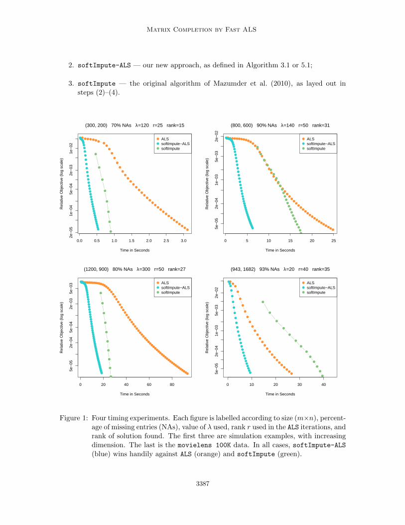
Figure 1 shows timing results on four datasets. The first three are simulation datasets ofincreasing size, and the last is the publicly available MovieLens 100K data. These experi-ments were all run in R using the softImpute package; see Section 7. Three methods arecompared:

1. ALS— Alternating Least Squares as in Algorithm 5.2;

3. Convergence is measured in terms of the usual notion of distance between subspaces (Golub and VanLoan, 2012); and it is also assumed that the initialization is not completely orthogonal to the targetsubspace, which is typically met in practice due to the presence of round-off errors.

3386


2. softImpute-ALS — our new approach, as defined in Algorithm 3.1 or 5.1;

3. softImpute — the original algorithm of Mazumder et al. (2010), as layed out insteps (2)–(4).

0.0 0.5 1.0 1.5 2.0 2.5 3.0

2e−

051e

−04

5e−

042e

−03

1e−

02

Time in Seconds

Rel

ativ

e O

bjec

tive

(log

scal

e)

ALSsoftImpute−ALSsoftImpute

(300, 200) 70% NAs λ=120 r=25 rank=15

0 5 10 15 20 25

5e−

052e

−04

1e−

035e

−03

2e−

02

Time in Seconds

Rel

ativ

e O

bjec

tive

(log

scal

e)


(800, 600) 90% NAs λ=140 r=50 rank=31

0 20 40 60 80

5e−

052e

−04

5e−

042e

−03

5e−

03

Time in Seconds

Rel

ativ

e O

bjec

tive

(log

scal

e)


(1200, 900) 80% NAs λ=300 r=50 rank=27

0 10 20 30 40

5e−

052e

−04

1e−

035e

−03

2e−

02

Time in Seconds

Rel

ativ

e O

bjec

tive

(log

scal

e)


(943, 1682) 93% NAs λ=20 r=40 rank=35

Figure 1: Four timing experiments. Each figure is labelled according to size (m×n), percent-age of missing entries (NAs), value of λ used, rank r used in the ALS iterations, andrank of solution found. The first three are simulation examples, with increasingdimension. The last is the movielens 100K data. In all cases, softImpute-ALS(blue) wins handily against ALS (orange) and softImpute (green).

3387


We used an R implementation for each of these in order to make the fairest comparisons.In particular, algorithm softImpute requires a low-rank SVD of a complete matrix at eachiteration. For this we used the function svd.als from our package, which uses alternatingsubspace iterations, rather than using other optimized code that is available for this task.Likewise, there exists optimized code for regular ALS for matrix completion, but instead weused our R version to make the comparisons fairer. We are trying to determine how thecomputational trade-offs play off, and thus need a level playing field.

Each subplot in Figure 6.1 is labeled according to the size of the problem, the fractionmissing, the value of λ used, the operating rank of the algorithms r, and the rank of thesolution obtained. All three methods involve alternating subspace methods; the first twoare alternating ridge regressions, and the third alternating orthogonal regressions. Theseare conducted at the operating rank r, anticipating a solution of smaller rank. Uponconvergence, softImpute-ALS performs step (5) in Algorithm 3.1, which can truncate therank of the solution. Our implementation of ALS does the same.

For the three simulation examples, the data are generated from an underlying Gaussianfactor model, with true ranks 50, 100, 100; the missing entries are then chosen at random.Their sizes are (300, 200), (800, 600) and (1200, 900) respectively, with between 70–90%missing. The MovieLens 100K data has 100K ratings (1–5) for 943 users and 1682 movies,and hence is 93% missing.

We picked a value of λ for each of these examples (through trial and error) so that thefinal solution had rank less than the operating rank. Under these circumstances, the solutionto the criterion (6) coincides with the solution to (1), which is unique under non-degeneratesituations.

There is a fairly consistent message from each of these experiments. softImpute-ALS

wins handily in each case, and the reasons are clear:

• Even though it uses more iterations than ALS, they are much cheaper to execute (bya factor O(r)).

• softImpute wastes time on its early SVD, even though it is far from the solution.Thereafter it uses warm starts for its SVD calculations, which speeds each step up,but it does not catch up.

6.2 Netflix Competition Data

We used our softImpute package in R to fit a sequence of models on the Netflix competitiondata. Here there are 480,189 users, 17,770 movies and a total of 100,480,507 ratings, makingthe resulting matrix 98.8% missing. There is a designated test set (the “probe set”), a subsetof 1,408,395 of the these ratings, leaving 99,072,112 for training.

Figure 2 compares the performance of hardImpute (Mazumder et al., 2010) with softImpute-ALS

on these data. hardImpute uses rank-restricted SVDs iteratively to estimate the missingdata, similar to softImpute but without shrinkage. The shrinkage helps here, leading toa best test-set RMSE of 0.943. This is a 1% improvement over the “Cinematch” score,somewhat short of the prize-winning improvement of 10%.

Both methods benefit greatly from using warm starts. hardImpute is solving a non-convex problem, while the intention is for softImpute-ALS to solve the convex problem

3388


0 50 100 150 200

0.7

0.8

0.9

1.0

Rank

RM

SE

TrainTest

0.65 0.70 0.75 0.80 0.85 0.90

0.95

0.96

0.97

0.98

0.99

1.00

Training RMSETe

st R

MS

E

hardImputesoftImpute−ALS

Netflix Competition Data

Figure 2: Performance of hardImpute versus softImpute-ALS on the Netflix data.hardImpute uses a rank-restricted SVD at each step of the imputation, whilesoftImpute-ALS does shrinking as well. The left panel shows the training andtest error as a function of the rank of the solution—an imperfect calibration inlight of the shrinkage. The right panel gives the test error as a function of thetraining error. hardImpute fits more aggressively, and overfits far sooner thansoftImpute-ALS. The horizontal dotted line is the “Cinematch” score, the targetto beat in this competition.

(1). This will be achieved if the operating rank is sufficiently large. The idea is to decide ona decreasing sequence of values for λ, starting from λmax (the smallest value for which the

solution M = 0, which corresponds to the largest singular value of PΩ(X)). Then for eachvalue of λ, use an operating rank somewhat larger than the rank of the previous solution,with the goal of getting the solution rank smaller than the operating rank. The sequenceof twenty models took under six hours of computing on a Linux cluster with 300Gb of ram(with a fairly liberal relative convergence criterion of 0.001), using the softImpute packagein R.

Figure 3 (left panel) gives timing comparison results for one of the Netflix fits, this timeimplemented in Matlab. The right panel gives timing results on the smaller MovieLens10M matrix. In these applications we need not get a very accurate solution, and so earlystopping is an attractive option. softImpute-ALS reaches a solution close to the minimumin about 1/4 the time it takes ALS.

3389


0 5 10 15

2e−

041e

−03

5e−

035e

−02

5e−

01

Time in Hours

Rel

ativ

e O

bjec

tive

(log

scal

e)

Netflix (480K, 18K) λ=100 r=100

ALSsoftImpute−ALS

0 10 20 30 40 50 60

5e−

055e

−04

5e−

035e

−02

5e−

01

Time in MinutesR

elat

ive

Obj

ectiv

e (lo

g sc

ale)

MovieLens 10M (72K, 10K) λ=50 r=100

Figure 3: Left: timing results on the Netflix matrix, comparing ALS with softImpute-ALS.Right: timing on the MovieLens 10M matrix. In both cases we see that whileALS makes bigger gains per iteration, each iteration is much more costly.

7. R Package softImpute

We have developed an R package softImpute for fitting these models (Hastie and Mazumder,2013), which is available on CRAN. The package implements both softImpute and softImpute-ALS.It can accommodate large matrices if the number of missing entries is correspondingly large,by making use of sparse-matrix formats. There are functions for centering and scaling (seeSection 9), and for making predictions from a fitted model. The package also has a functionsvd.als for computing a low-rank SVD of a large sparse matrix, with row and/or columncentering. More details can be found in the package Vignette on the first authors web page,at

http://web.stanford.edu/~hastie/swData/softImpute/vignette.html.

8. Distributed Implementation

We provide a distributed version of softimpute-ALS (given in Algorithm 5.1), built uponthe Spark cluster programming framework.

8.1 Design

The input matrix to be factored is split row-by-row across many machines. The transposeof the input is also split row-by-row across the machines. The current model (i.e. the

3390

http://web.stanford.edu/~hastie/swData/softImpute/vignette.html


current guess for A,B) is repeated and held in memory on every machine. Thus the totaltime taken by the computation is proportional to the number of non-zeros divided by thenumber of CPU cores, with the restriction that the model should fit in memory.

At every iteration, the current model is broadcast to all machines, such that there isonly one copy of the model on each machine. Each CPU core on a machine will processa partition of the input matrix, using the local copy of the model available. This meansthat even though one machine can have many cores acting on a subset of the input data,all those cores can share the same local copy of the model, thus saving RAM. This savingis especially pronounced on machines with many cores.

The implementation is available online at http://git.io/sparkfastals with docu-mentation, in Scala. The implementation has a method named multByXstar, correspondingto line 3 of Algorithm 5.1 which multiplies X∗ by another matrix on the right, exploitingthe “sparse-plus-low-rank” structure of X∗. This method has signature:

multByXstar(X: IndexedRowMatrix, A: BDM[Double], B: BDM[Double], C:

BDM[Double])

This method has four parameters. The first parameter X is a distributed matrix consistingof the input, split row-wise across machines. The full documentation for how this matrix isspread across machines is available online4. The multByXstar method takes a distributedmatrix, along with local matrices A, B, and C, and performs line 3 of Algorithm 5.1 bymultiplying X∗ by C. Similarly, the method multByXstarTranspose performs line 5 ofAlgorithm 5.1.

After each call to multByXstar, the machines each will have calculated a portion of A.Once the call finishes, the machines each send their computed portion (which is small andcan fit in memory on a single machine, since A can fit in memory on a single machine) tothe master node, which will assemble the new guess for A and broadcast it to the workermachines. A similar process happens for multByXstarTranspose, and the whole process isrepeated every iteration.

8.2 Experiments

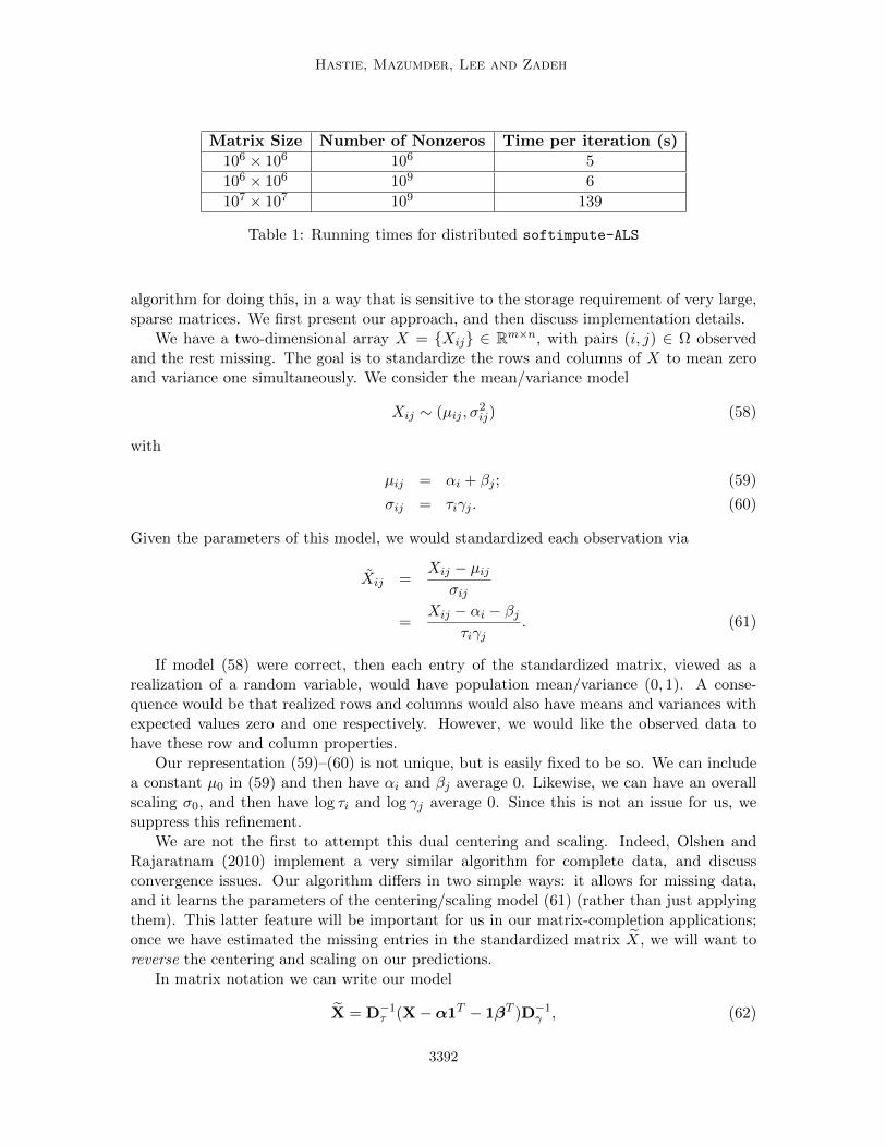
We report iteration times using an Amazon EC2 cluster with 10 slaves and one master, ofinstance type “c3.4xlarge”. Each machine has 16 CPU cores and 30 GB of RAM. We ransoftimpute-ALS on matrices of varying sizes with iteration runtimes available in Table 1,setting k = 5. Where possible, hardware acceleration was used for local linear algebraicoperations, via breeze and BLAS.

The popular Netflix prize matrix has 17, 770 rows, 480, 189 columns, and 100, 480, 507non-zeros. We report results on several larger matrices in Table 1, up to 10 times larger.

9. Centering and Scaling

We often want to remove row and/or column means from a matrix before performing alow-rank SVD or running our matrix completion algorithms. Likewise we may wish tostandardize the rows and or columns to have unit variance. In this section we present an

4. https://spark.apache.org/docs/latest/mllib-basics.html#indexedrowmatrix

3391

http://git.io/sparkfastals

https://spark.apache.org/docs/latest/mllib-basics.html#indexedrowmatrix


Matrix Size Number of Nonzeros Time per iteration (s)

106 × 106 106 5

106 × 106 109 6

107 × 107 109 139

Table 1: Running times for distributed softimpute-ALS

algorithm for doing this, in a way that is sensitive to the storage requirement of very large,sparse matrices. We first present our approach, and then discuss implementation details.

We have a two-dimensional array X = Xij ∈ Rm×n, with pairs (i, j) ∈ Ω observedand the rest missing. The goal is to standardize the rows and columns of X to mean zeroand variance one simultaneously. We consider the mean/variance model

Xij ∼ (µij , σ2ij) (58)

with

µij = αi + βj ; (59)

σij = τiγj . (60)

Given the parameters of this model, we would standardized each observation via

Xij =Xij − µij

σij

=Xij − αi − βj

τiγj. (61)

If model (58) were correct, then each entry of the standardized matrix, viewed as arealization of a random variable, would have population mean/variance (0, 1). A conse-quence would be that realized rows and columns would also have means and variances withexpected values zero and one respectively. However, we would like the observed data tohave these row and column properties.

Our representation (59)–(60) is not unique, but is easily fixed to be so. We can includea constant µ0 in (59) and then have αi and βj average 0. Likewise, we can have an overallscaling σ0, and then have log τi and log γj average 0. Since this is not an issue for us, wesuppress this refinement.

We are not the first to attempt this dual centering and scaling. Indeed, Olshen andRajaratnam (2010) implement a very similar algorithm for complete data, and discussconvergence issues. Our algorithm differs in two simple ways: it allows for missing data,and it learns the parameters of the centering/scaling model (61) (rather than just applyingthem). This latter feature will be important for us in our matrix-completion applications;once we have estimated the missing entries in the standardized matrix X, we will want toreverse the centering and scaling on our predictions.

In matrix notation we can write our model

X = D−1τ (X−α1T − 1βT )D−1

γ , (62)

3392


where Dτ = diag(τ1, τ2, . . . , τm), similar for Dγ , and the missing values are represented inthe full matrix as NAs (e.g. as in R). Although it is not the focus of this paper, this centeringmodel is also useful for large, complete, sparse matrices X (with many zeros, stored in sparse-matrix format). Centering would destroy the sparsity, but from (62) we can see we can storeit in “sparse-plus-low-rank” format. Such a matrix can be left and right-multiplied easily,and hence is ideal for alternating subspace methods for computing a low-rank SVD. Thefunction svd.als in the softImpute package (section 7) can accommodate such structure.

9.1 Method-of-moments Algorithm

We now present an algorithm for estimating the parameters. The idea is to write down foursystems of estimating equations that demand that the transformed observed data have rowmeans zero and variances one, and likewise for the columns. We then iteratively solve theseequations, until all four conditions are satisfied simultaneously. We do not in general haveany guarantees that this algorithm will always converge except in the noted special cases,but empirically we typically see rapid convergence.

Consider the estimating equation for the row-means condition (for each row i)

1

ni

∑j∈Ωi

Xij =1

ni

∑j∈Ωi

Xij − αi − βjτiγj

(63)

= 0,

where Ωi = j|(i, j) ∈ Ω, and ni = |Ωi| ≤ n. Rearranging we get

αi =

∑j∈Ωi

1γj

(Xij − βj)∑j∈Ωi

1γj

, i = 1, . . . ,m. (64)

This is a weighted mean of the partial residuals Xij−βj with weights inversely proportionalto the column standard-deviation parameters γj . By symmetry, we get a similar equationfor βj ,

βj =

∑i∈Ωj

1τi

(Xij − αi)∑i∈Ωj

1τi

, j = 1, . . . , n, (65)

where Ωj = i|(i, j) ∈ Ω, and mj = |Ωj | ≤ m.Similarly, the variance conditions for the rows are

1

ni

∑j∈Ωi

X2ij =

1

ni

∑j∈Ωi

(Xij − αi − βj)2

τ2i γ

2j

(66)

= 1,

which simply says

τ2i =

1

ni

∑j∈Ωi


γ2j

, i = 1, . . . ,m. (67)

Likewise

γ2j =

1

mj

∑i∈Ωj


τ2i

, j = 1, . . . , n. (68)

3393


The method-of-moments estimators require iterating these four sets of equations (64), (65),(67), (68) till convergence. We monitor the following functions of the “residuals”

R =m∑i=1

1

ni

∑j∈Ωi

Xij

2

+n∑j=1

1

mj

∑i∈Ωj

Xij

2

(69)

+m∑i=1

log2

1

ni

∑j∈Ωi

X2ij

+n∑j=1

log2

1

mj

∑i∈Ωj

X2ij

(70)

In experiments it appears that R converges to zero very fast, perhaps linear convergence. InAppendix B we show slightly different versions of these estimators which are more suitablefor sparse-matrix calculations.

In practice we may not wish to apply all four standardizations, but instead a subset.For example, we may wish to only standardize columns to have mean zero and variance one.In this case we simply set the omitted centering parameters to zero, and scaling parametersto one, and skip their steps in the iterative algorithm. In certain cases we have convergenceguarantees:

• Column-only centering and/or scaling. Here no iteration is required; the centeringstep precedes the scaling step, and we are done. Likewise for row-only.

• Centering only, no scaling. Here the situation is exactly that of an unbalanced two-way ANOVA, and our algorithm is exactly the Gauss-Seidel algorithm for fittingthe two-way ANOVA model. This is known to converge, modulo certain degeneratesituations.

For the other cases we have no guarantees of convergence.We present an alternative sequence of formulas in Appendix B which allows one to

simultaneously apply the transformations, and learn the parameters.

10. Discussion

We have presented a new algorithm for matrix completion, suitable for solving Problem (1)for very large problems, as long as the solution rank is manageably low. Our algorithmcapitalizes on the different strengths and weakness in each of the popular alternatives:

• ALS has to solve a different regression problem for every row/column, because of theirdifferent amount of missingness, and this can be costly. softImpute-ALS solves asingle regression problem once and simultaneously for all the rows/columns, becauseit operates on a filled-in matrix which is complete. Although these steps are typicallynot as strong as those of ALS, the speed advantage more than compensates.

• softImpute wastes time in early iterations computing a low-rank SVD of a far-from-optimal estimate, in order to make its next imputation. One can think ofsoftImpute-ALS as simultaneously filling in the matrix at each alternating step, asit is computing the SVD. By the time it is done, it has the the solution sought bysoftImpute, but with far fewer iterations.

3394


softImpute allows for an extremely efficient distributed implementation (Section 8), andhence can scale to large problems, given a sufficiently large computing infrastructure.

Acknowledgments

The authors thank Balasubramanian Narasimhan for helpful discussions on distributedcomputing in R. The first author thanks Andreas Buja and Stephen Boyd for stimulating“footnote” discussions that led to the centering/scaling in Section 9. Trevor Hastie waspartially supported by grant DMS-1407548 from the National Science Foundation, andgrant RO1-EB001988-15 from the National Institutes of Health. Rahul Mazumder wasfunded in part by Columbia University’s start-up funds and a grant from the Betty-MooreSloan Foundation.

Appendix A. Proofs from Section 5.1

Here, we gather some proofs and technical details from Section 5.1.

A.1 Proof of Lemma 2

To prove this we begin with the following elementary result concerning a ridge regressionproblem:

Lemma 5 Consider a ridge regression problem

H(β) := 12‖y −Mβ‖22 +

λ

2‖β‖22 (71)

with β∗ ∈ arg minβ H(β). Then the following inequality is true:

H(β)−H(β∗) =1

2(β − β∗)T (MTM + λI)(β − β∗) = 1

2‖M(β − β∗)‖22 +λ

2‖β − β∗‖22

Proof The proof follows from the second order Taylor Series expansion of H(β):

H(β) = H(β∗) + 〈∇H(β∗), β − β∗〉+1

2(β − β∗)T (MTM + λI)(β − β∗)

and observing that ∇H(β∗) = 0.

3395


We will need to obtain a lower bound on the difference F (Ak+1, Bk) − F (Ak, Bk). To-wards this end we make note of the following chain of inequalities:

F (Ak, Bk) = g(AkBTk ) +

λ

2(‖Ak‖2F + ‖Bk‖2F ) (72)

= QA(Ak|Ak, Bk) (73)

≥ minZ1

QA(Z1|Ak, Bk) (74)

= QA(Ak+1|Ak, Bk) (75)

≥ g(Ak+1BTk ) +

λ

2(‖Ak+1‖2F + ‖Bk‖2F ) (76)

= F (Ak+1, Bk) (77)

where, Line (73) follows from (31), and (76) follows from (30).Clearly, from Lines (77) and (72) we have (78)

F (Ak, Bk)− F (Ak+1, Bk) ≥ QA(Ak|Ak, Bk)−QA(Ak+1|Ak, Bk) (78)

= 12‖(Ak+1 −Ak)BT

k ‖22 +λ

2‖Ak+1 −Ak‖22, (79)

where, (79) follows from (78) using Lemma 5.Similarly, following the above steps for the B-update we have:

F (Ak, Bk)− F (Ak+1, Bk+1) ≥ 12‖Ak+1(Bk+1 −Bk)T ‖22 +

λ

2‖Bk+1 −Bk‖22. (80)

Adding (79) and (80) we get (35) concluding the proof of the lemma.

A.2 Proof of Lemma 3

Let us use the shorthand ∆ in place of ∆ ((A,B) , (A+, B+)) as defined in (37).First of all observe that the result (35) can be replaced with (Ak, Bk) ← (A,B) and

(Ak+1, Bk+1)← (A+, B+). This leads to the following:

F (A,B)− F (A+, B+) ≥ 12

(‖(A−A+)BT ‖2F + ‖A+(B+ −B)T ‖2F

)+λ

2

(‖A−A+‖2F + ‖B+ −B‖2F

).

(81)

First of all, it is clear that if A,B is a fixed point then ∆ = 0.Let us consider the converse, i.e., the case when ∆ = 0. Note that if ∆ = 0 then each of

the summands appearing in the definition of ∆ is also zero. We will now make use of theinteresting result (that follows from the Proof of Lemma 2) in (78) and (79) which says:

QA(A|A,B)−QA(A+|A,B) = 12‖(A

+ −A)BT ‖22 +λ

2‖A+ −A‖22.

Now the right hand side of the above equation is zero (since ∆ = 0) which implies that,QA(A|A,B)−QA(A+|A,B) = 0. An analogous result holds true for B.

Using the nesting property (34), it follows that F (A,B) = F (A+, B+)—thereby showingthat (A,B) is a fixed point of the algorithm.

3396


A.3 Proof of Theorem 4

We make use of (35) and add both sides of the inequality over k = 1, . . . ,K, which leadsto:

K∑i=1

(F (Ak, Bk)− F (Ak+1, Bk+1)) ≥K∑k=1

ηk ≥ K( minK≥k≥1

ηk) (82)

Since, F (Ak, Bk) is a decreasing sequence (bounded below) it converges to F∞ say. Itfollows that:

K∑i=1

(F (Ak, Bk)− F (Ak+1, Bk+1)) = F (A1, B1)− F (AK+1, BK+1)

≤ F (A1, B1)− F∞(83)

Using (83) along with (82) we have the following convergence rate:

min1≤k≤K

ηk ≤(F (A1, B1)− F (A∞, B∞)

)/K,

thereby completing the proof of the theorem.

A.4 Proof of Corollary 1

Recall the definition of ηk

ηk = 12

(‖(Ak −Ak+1)BT

k ‖2F + ‖Ak+1(Bk −Bk+1)T ‖2F)+λ

2

(‖Ak −Ak+1‖2F + ‖Bk −Bk+1‖2F

)Since we have assumed that

ÙI BTk Bk `LI, ÙI ATkAk `LI, ∀k

we then have:

ηk ≥(`L

2+λ

2

)‖Ak −Ak+1‖2F +

(`L

2+λ

2

)‖Bk −Bk+1‖2F .

Using the above in (82) and assuming that `L > 0, we have the bound:

min1≤k≤K

(‖(Ak −Ak+1)‖2F + ‖Bk −Bk+1‖2F

)≤ 2

(`L + λ)

(F (A1, B1)− F∞

K

)(84)

Suppose instead of the proximity measure:(‖(Ak −Ak+1)‖2F + ‖Bk −Bk+1‖2F

),

we use the proximity measure:(‖(Ak −Ak+1)BT

k ‖2F + ‖Ak+1(Bk −Bk+1)‖2F).

Then observing that:

Ù‖(Ak −Ak+1)‖2F ≥ ‖(Ak −Ak+1)BTk ‖2F , Ù‖Bk −Bk+1‖2F ≥ ‖Ak+1(Bk −Bk+1)T ‖2F

3397


we have:

ηk ≥(

λ

2Ù+

1

2

)(‖(Ak −Ak+1)BT

k ‖2F + ‖Ak+1(Bk −Bk+1)‖2F).

Using the above bound in (82) we arrive at a bound which is similar in spirit to (41) butwith a different proximity measure on the step-sizes:

min1≤k≤K

(‖(Ak −Ak+1)BT

k ‖2F + ‖Ak+1(Bk −Bk+1)‖2F)≤ 2Ù

λ+ Ù

(F (A1, B1)− F∞

K

)(85)

It is useful to contrast results (41) and (42) with the case λ = 0.

min1≤k≤K

(‖(Ak −Ak+1)BT

k ‖2F + ‖Ak+1(Bk −Bk+1)‖2F)≤

2Ù

λ+Ù

(F (A1,B1)−F∞

K

)λ > 0

2Ù(F (A1,B1)−F∞

K

)λ = 0

(86)The convergence rate with the other proximity measure on the step-sizes have the followingtwo cases:

min1≤k≤K

(‖(Ak −Ak+1)‖2F + ‖Bk −Bk+1‖2F

)≤

2

(`L+λ)

(F (A1,B1)−F∞

K

)λ > 0,

2`L

(F (A1,B1)−F∞

K

)λ = 0.

(87)

The assumption (40) ÙI BTk Bk and ÙI ATkAk can be interpreted as an upper

bounds to the locally Lipschitz constants of the gradients ofQA(Z|Ak, Bk) andQB(Z|Ak+1, Bk)for all k:

‖∇QA(Ak+1|Ak, Bk)−∇QA(Ak|Ak, Bk)‖ ≤ Ù‖Ak+1 −Ak‖,‖∇QB(Bk|Ak+1, Bk)−∇QB(Bk+1|Ak+1, Bk)‖ ≤ Ù‖Bk+1 −Bk‖.

(88)

The above leads to convergence rate bounds on the (partial) gradients of the functionF (A,B), i.e.,

min1≤k≤K

(‖∇Af(Ak, Bk)‖2 + ‖∇Bf(Ak+1, Bk)‖2

)≤ 2(Ù )2

(`L + λ)

(F (A1, B1)− F∞

K

)A.5 Proof of Theorem 5

Proof Part (a):We make use of the convergence rate derived in Theorem 4. As k → ∞, it follows thatηk → 0. This describes the fate of the objective values F (Ak, Bk), but does not inform usabout the properties of the sequence Ak, Bk. Towards this end, note that if λ > 0, then thesequence Ak, Bk is bounded and thus has a limit point. Let A∗, B∗ be any limit point of thesequence Ak, Bk. It follows by a simple subsequence argument that F (Ak, Bk)→ F (A∗, B∗)and A∗, B∗ is a fixed point of Algorithm 5.1 and in particular a first order stationary pointof Problem (6).Part (b):The sequence (Ak, Bk) need not have a unique limit point, however, we show below: forevery subsequence of Bk that converges, the corresponding subsequence of Ak also converges.

3398


Suppose, Bk → B∗ (along a subsequence k ∈ ν). We will show that the sequence Ak fork ∈ ν has a unique limit point.

We argue by the method of contradiction. Suppose there are two limit points of Ak, k ∈ν, namely, A1 and A2 and Ak1 → A1, k1 ∈ ν1 ⊂ ν and Ak2 → A2, k2 ∈ ν2 ⊂ ν with A1 6= A2.

Consider the objective value sequence: F (Ak, Bk). For fixed Bk the update in A fromAk to Ak+1 results in

F (Ak, Bk)− F (Ak+1, Bk) ≥λ

2‖Ak −Ak+1‖2F .

Take k1 ∈ ν1 and k2 ∈ ν2, we have:

F (Ak2 , Bk2)− F (Ak1+1, Bk1) = (F (Ak2 , Bk2)− F (Ak2 , Bk1))

+ (F (Ak2 , Bk1)− F (Ak1+1, Bk1)) (89)

≥ (F (Ak2 , Bk2)− F (Ak2 , Bk1)) +λ

2‖Ak2 −Ak1+1‖2F (90)

where Line 90 follows by using Lemma 5. As k1, k2 →∞, Bk2 , Bk1 → B∗ hence,

F (Ak2 , Bk2)− F (Ak2 , Bk1)→ 0, and ‖Ak2 −Ak1+1‖2F → ‖A2 −A1‖2F

However, the lhs of (89) converges to zero, which is a contradiction. This implies that‖A2 −A1‖2F = 0 i.e. Ak for k ∈ ν has a unique limit point.

Exactly the same argument holds true for the sequence Ak, leading to the conclusion ofthe other part of Part (b).

Appendix B. Alternative Computing Formulas for Method of Moments

In this section we present the same algorithm, but use a slightly different representation.For matrix-completion problems, this does not make much of a difference in terms of com-putational load. But we also have other applications in mind, where the large matrix Xmay be fully observed, but is very sparse. In this case we do not want to actually apply thecentering operations; instead we represent the matrix as a “sparse-plus-low-rank” object, aclass for which we have methods for simple row and column operations.

Consider the row-means (for each row i). We can introduce a change ∆αi from the old

αoi to the new αi. Then we have∑j∈Ωi

Xij =∑j∈Ωi

Xij − αoi −∆αi − βj

τiγj(91)

= 0,

where as before Ωi = j|(i, j) ∈ Ω. Rearranging we get

∆αi =

∑j∈Ωi

Xoij∑

j∈Ωi

1τiγj

, i = 1, . . . ,m, (92)

3399


where

Xoij =

Xij − αoi − βjτiγj

. (93)

Then αi = αoi + ∆αi . By symmetry, we get a similar equation for ∆β

j ,

Likewise for the variances.

1

ni

∑j∈Ωi

X2ij =

1

ni

∑j∈Ωi


(τi∆τi )2γ2

j

(94)

=1

ni

∑j∈Ωi

(Xoij

∆τi

)2

(95)

= 1.

Here we modify τi by a multiplicative factor ∆τi . Here the solution is

(∆τi )2 =

1

ni

∑j∈Ωi

(Xoij)

2, i = 1, . . . ,m. (96)

By symmetry, we get a similar equation for ∆γj ,

The method-of-moments estimators amount to iterating these four sets of equations tillconvergence. Now we can monitor the changes via

R =m∑i=1

∆αi

2 +n∑j=1

∆βj

2+

m∑i=1

log2 ∆τi +

n∑j=1

log2 ∆γj (97)

which should converge to zero.

References

Dimitri P Bertsekas. Nonlinear Programming. Athena Scientific, Belmont, Massachusetts,2nd edition, 1999. ISBN 1886529000. URL http://www.amazon.com/exec/obidos/

redirect?tag=citeulike07-20&path=ASIN/1886529000.

Samuel Burer and Renato D.C. Monteiro. Local minima and convergence in low-ranksemidefinite programming. Mathematical Programming, 103(3):427–631, 2005.

Emmanuel Candes and Benjamin Recht. Exact matrix completion via convex optimization.Foundations of Computational Mathematics, 2008. doi: 10.1007/s10208-009-9045-5. URLhttp://dx.doi.org/10.1007/s10208-009-9045-5.

Emmanuel J. Candes and Terence Tao. The power of convex relaxation: Near-optimalmatrix completion, 2009. URL http://www.citebase.org/abstract?id=oai:arXiv.

org:0903.1476.

Caihua Chen, Bingsheng He, and Xiaoming Yuan. Matrix completion via an alternatingdirection method. IMA Journal of Numerical Analysis, 32(1):227–245, 2012.

3400

http://www.amazon.com/exec/obidos/redirect?tag=citeulike07-20&path=ASIN/1886529000


http://dx.doi.org/10.1007/s10208-009-9045-5

http://www.citebase.org/abstract?id=oai:arXiv.org:0903.1476

http://www.citebase.org/abstract?id=oai:arXiv.org:0903.1476


G. Golub and C. Van Loan. Matrix Computations. Johns Hopkins University Press, 3edition, 2012.

Moritz Hardt. Understanding alternating minimization for matrix completion. In Foun-dations of Computer Science (FOCS), 2014 IEEE 55th Annual Symposium on, pages651–660. IEEE, 2014.

Trevor Hastie and Rahul Mazumder. softImpute: Matrix Completion via Iterative Soft-Thresholded Svd, 2013. URL http://CRAN.R-project.org/package=softImpute. Rpackage version 1.0.

Trevor Hastie, Robert Tibshirani, and Jerome Friedman. The Elements of Statistical Learn-ing, Second Edition: Data Mining, Inference, and Prediction (Springer Series in Statis-tics). Springer New York, 2 edition, 2009. ISBN 0387848576.

Prateek Jain, Praneeth Netrapalli, and Sujay Sanghavi. Low-rank matrix completion usingalternating minimization. In Proceedings of the Forty-Fifth Annual ACM Symposium onTheory of Computing, pages 665–674. ACM, 2013.

Michel Journee, F Bach, P-A Absil, and Rodolphe Sepulchre. Low-rank optimization on thecone of positive semidefinite matrices. SIAM Journal on Optimization, 20(5):2327–2351,2010.

Yehuda Koren, Robert Bell, and Chris Volinsky. Matrix factorization techniques for recom-mender systems. Computer, 42(8):30–37, 2009.

R.M. Larsen. Propack-software for large and sparse svd calculations, 2004. URL http:

//sun.stanford.edu/~rmunk/PROPACK/.

A. Lewis. Derivatives of spectral functions. Mathematics of Operations Research, 21(3):576–588, 1996.

Rahul Mazumder, Trevor Hastie, and Rob Tibshirani. Spectral regularization algorithms forlearning large incomplete matrices. Journal of Machine Learning Research, 11:2287–2322,2010.

Leon Mirsky. A trace inequality of John von Neumann. Monatshefte fur Mathematik, 79(4):303–306, 1975.

Richard Olshen and Bala Rajaratnam. Successive normalization of rectangular arrays.Annals of Statistics, 38(3):1638–1664, 2010.

Meisam Razaviyayn, Mingyi Hong, and Zhi-Quan Luo. A unified convergence analysis ofblock successive minimization methods for nonsmooth optimization. SIAM Journal onOptimization, 23(2):1126–1153, 2013.

J. Rennie and N. Srebro. Fast maximum margin matrix factorization for collaborativeprediction. In ICML, 2005.

Nathan Srebro, Jason Rennie, and Tommi Jaakkola. Maximum margin matrix factorization.Advances in Neural Information Processing Systems, 17, 2005.

3401

http://CRAN.R-project.org/package=softImpute

http://sun.stanford.edu/~rmunk/PROPACK/

http://sun.stanford.edu/~rmunk/PROPACK/


G. Stewart and Ji-Guang Sun. Matrix Perturbation Theory. Academic Press, Boston, 1 edi-tion, 1990. ISBN 0126702306. URL http://www.amazon.com/exec/obidos/redirect?

tag=citeulike07-20&path=ASIN/0126702306.

Yunhong Zhou, Dennis Wilkinson, Robert Schreiber, and Rong Pan. Large-scale parallelcollaborative filtering for the netflix prize. In Algorithmic Aspects in Information andManagement, pages 337–348. Springer, 2008.

3402



Documents

Matrix Completion and Low-Rank SVD via Fast Alternating