Seediscussions,stats,andauthorprofilesforthispublicationat:https://www.researchgate.net/publication/286649267

MatrixAlgebraTopicsinStatisticsandEconomicsUsingR

ArticleinHandbookofStatistics·December2014

DOI:10.1016/B978-0-444-63431-3.00004-8

CITATIONS

0

READS

189

1author:

HrishikeshD.Vinod

FordhamUniversity

158PUBLICATIONS2,211CITATIONS

SEEPROFILE

Allin-textreferencesunderlinedinbluearelinkedtopublicationsonResearchGate,

lettingyouaccessandreadthemimmediately.

Availablefrom:HrishikeshD.Vinod

Retrievedon:20September2016

Matrix Algebra Topics in Statistics andEconomics Using R

Hrishikesh D. Vinod∗

October 20, 2014

Abstract

This chapter provides a review of certain matrix algebra topicsuseful in Economics and Statistics which can be implemented by us-ing the R software and graphics system. We illustrate uses of newerversions of R packages including graphics for visualization of rela-tions. In addition to basics we include newer innovative topics havingpractical relevance including decision payoff matrices, new generalizedasymmetric correlations, sparse matrices, heteroscedasticity and auto-correlation consistent (HAC) covariance matrices, projection matrices,robust multivariate outlier detection tools, generalized canonical cor-relations, demographic transitions and others.

1 Introduction

This chapter discusses some results from matrix algebra used in Statisticsand Econometrics, where the use of the free R software and graphics systemis feasible. An aim of this chapter is to facilitate learning of the matrix theoryand its applications using R software tools. There are many books for matrixalgebra including Gantmacher (1959), Rao (1973). With the wide availabilityof the Internet, the open source and free R software has attracted researchersfrom around the world allowing for exponential growth in the number of users

∗Vinod: Professor of Economics, Fordham University, Bronx, New York, USA 10458.E-mail: vinod@fordham.edu.

1

of R. To the best of my knowledge, the first matrix algebra book using R isVinod (2011).

It is impossible to review thousands of matrix algebra tools scatteredover thousands of R packages in a single chapter. We focus on those toolsfrom only a few packages which are important in Statistics and Economicsand which deserve attention. We assume that the reader has some familiaritywith basics of R including downloading of packages from CRAN and bringingthem into current memory with the ‘require’ command.

Official R uses as the assignment symbol “ <- ” which requires fourstrokes, since it generally needs to be surrounded by spaces to avoid con-fusion. Fortunately, R (similar to FORTRAN) allows us to use an alternatesymbol “=” for assignment, which requires only one stroke and no surround-ing spaces. Hence, I will use the shorter assignment symbol to save printingspace throughout, even though my code may not be portable to S-plus. Afterall, a global search for ‘=’ and replacement with “ <- ” except in functiondefaults is not hard.

An R session should begin, in my opinion, with the following code whichremoves the R prompt ‘>’ completely and replaces the ‘+’ used by R for‘continuation of command’ symbol with two blank spaces to permit directcopy and paste from any electronic copy of this chapter. Since R ignoreseverything after the # symbol in a command line, we often use it throughoutthis chapter to explain the meaning of individual R commands.

#snippet cleanup

rm(list=ls()) #clean out memory

options(prompt = " ", continue = " ", width = 68,

useFancyQuotes = FALSE) #my recommended options

print(date()) #date stamp

The outline of the remaining chapter is as follows. Section 2 begins withbasic matrix manipulations in R, followed by Section 3 for descriptive statis-tics. Section 4 reviews invariance and equivariance under affine tranforma-tions. Section 5 reviews my chapter 5 dealing with decision analysis from mybook Vinod (2011). By providing a link to my R software we are able to savespace in this section. Section 6 considers matrix algebra in regression models.Section 7 focuses on the correlation matrix and describes a new generalizedcorrelation matrix for assessment of potential causality, while relaxing thelinearity assumption as explained in my paper, Vinod (2013). Section 8 dis-cusses matrices in study of population dynamics, while section 9 describes

2

multivariate component analysis. Section 10 deals with R tools for workingwith sparse matrices.

2 Basic Matrix Manipulations in R

We illustrate some matrix algebra concepts in R by using Motor Trend maga-zine’s automobile engineering specifications data for 32 automobiles discussedin Henderson and Velleman (1981) and elsewhere. The data is called ‘mtcars,’and is always available in R by that name. The command ‘names(mtcars)’will list the names of all 11 variables. The command ‘attach(mtcars)’ al-lows us to treat each name as a 32×1 vector representing the variable. TheR function ‘cbind’ stands for ‘column binding’ of vectors into a matrix.

names(mtcars)

attach(mtcars)

A=cbind(mpg,disp,hp);A #32 by 3 matrix

B=cbind(drat,wt,qsec);B#32 by 3 matrix

The reader should type ‘?mtcars’ to obtain detailed information aboutthe cars data and meaning of all symbols such as miles per gallon (mpg),horsepower (hp) and weight (wt). The last two lines from the above codehave the ‘cbind’ function which “column binds” the indicated three variablesinto our A and B matrices. The names are accessible thanks to the ‘attach’command.

Additional information about any R function is found by typing ?anyfn

without spaces after the ‘?’ at the R console.

Bd=t(B);Bd #B dash=transpose of B, so Bd is 3 by 32

Bd %*% A #row column matrix multiplication

crossprod(B,A) #cross product B'A of two matrices

The transpose of B is defined by the code ‘Bd=t(B),’ which is a 3×32 matrix.The row-column matrix multiplication of Bd with A is given by the command(Bd %*% A) to yield a 3×3 matrix saved by us in the R object called ‘BdA’in the following code: Note that typing ?"%*%" without any spaces andwith quotes, gives details about the set of three symbols in R for matrixmultiplication. Matrix multiplication of two vectors gives their inner product.

3

Verify that the R function ‘crossprod’ is a convenient replacement ofthe code ‘(Bd %*% A),’ since both commands give same answer. In fact,‘crossprod’ is numerically more reliable and more efficiently executed in Rthan the alternative. ‘crossprod(mpg,wt)’ gives the inner product of twovectors.

R has many more functions similar to ‘crossprod’ for matrix manipula-tions. An outer product of two n× 1 vectors (n=32 here) will be an n× nmatrix. It is given by the following code.

mpg %o% wt #32 by 32 outer product of two 32 by 1 vectors

Matrix Inverse of a square matrix is computed by the function ‘solve’in R.

cpAB=crossprod(A,B)#define crossprod 3 by 3 matrix

cpABInv=solve(cpAB) #create inverse matrix

round(cpABInv %*% cpAB,12) #this should be identity

We report only the last line verifying that the inverse matrix times the origi-nal square matrix is the identity matrix. We round the answer to 12 decimalspaces by the ‘round’ function on the last line of the code above.

drat wt qsec

drat 1 0 0

wt 0 1 0

qsec 0 0 1

If the original matrix is not square, similar to our ‘A,’ its usual inversedoes not exist. R has thousands of ‘packages’ which can be accessed free bythe command ‘library’ or ‘require’. The Moore-Penrose generalized (left)inverse of a matrix is readily computed by the function ‘ginv’ available inthe package ‘MASS’, Venables and Ripley (2002).

library(MASS) #access the package `MASS'

ginv(A) #3 by 32 Moore Penrose generalized inverse

round(ginv(A) %*% A, 12) #This is 3 by 3 identity matrix

The last line of the above code verifies that the pre-multiplication by theleft inverse yields the identity matrix. That is, the function ‘ginv’ is workingcorrectly.

4

3 Descriptive Statistics

The standard summary of data includes vectors of means, variances and otherdescriptive statistics obtained by the command ‘summary(A).’ I personallylike to use the function ‘basicStats’ from the package ‘fBasics.’

attach(mtcars)

A=cbind(mpg,disp,hp);A #32 by 3 matrix

head(A, 3)# view first 3 lines of A

summary(A)

require(fBasics)

b1=basicStats(A);b1

While we are suppressing some R outputs for brevity, we do include descrip-tive statistics provided by the function ‘basicStats’ reporting most descriptivecharacteristics of each column separately. It includes the sample size n alongthe row nobs, the number of missing data (NAs), lower and uppoer 95%confidence limits (LCL, UCL) of the mean, etc. with self-explanatory rownames.

head(A, 3)# view first 3 lines of A

mpg disp hp

[1,] 21.0 160 110

[2,] 21.0 160 110

[3,] 22.8 108 93

b1=basicStats(A);b1

mpg disp hp

nobs 32.0000 32.0000 32.0000

NAs 0.0000 0.0000 0.0000

Minimum 10.4000 71.1000 52.0000

Maximum 33.9000 472.0000 335.0000

1. Quartile 15.4250 120.8250 96.5000

3. Quartile 22.8000 326.0000 180.0000

Mean 20.0906 230.7219 146.6875

Median 19.2000 196.3000 123.0000

Sum 642.9000 7383.1000 4694.0000

SE Mean 1.0654 21.9095 12.1203

LCL Mean 17.9177 186.0372 121.9680

UCL Mean 22.2636 275.4065 171.4070

5

Variance 36.3241 15360.7998 4700.8669

Stdev 6.0269 123.9387 68.5629

Skewness 0.6107 0.3817 0.7260

Kurtosis -0.3728 -1.2072 -0.1356

Sample variance and covariance computation requires deviations from themean. The following R code begins with an ad hoc R function called ‘dev’ tocomputes deviations of arbitrary vector x from the mean. Next we use the‘apply’ function in R designed to avoid time-consuming loops. For example,‘apply(A, 2, dev)’ applies the ad hoc function ‘dev’ to the matrix object ‘A’where the second argument 2 means the second dimension (i.e., columns) ofthe matrix A. If the second argument were 1, it would operate on rows ofA. Our code defines a new matrix object called ‘demeanA’ which containsdeviations from the mean for each column of A.

dev=function(x)x-mean(x)

demeanA=apply(A, 2, dev)

head(demeanA, 3)

Top 3 lines of ‘demeanA’ are reported next.

mpg disp hp

[1,] 0.909375 -70.72188 -36.6875

[2,] 0.909375 -70.72188 -36.6875

[3,] 2.709375 -122.72188 -53.6875

The variance covariance matrix of the three variables is computed by thecode ‘cov(A).’ It can also be computed directly from our ‘demeanA’ matrixby using the ‘crossprod’ function and dividing by (n− 1) = 31 here.

cov1=cov(A)

n=NROW(A)

cov2=crossprod(demeanA)/(n-1)

diff=round((cov1-cov2),12)

max(diff)

The output of the above code is zero, showing that the two matrices cov1and cov2 are identical.

6

3.1 Outlier detection and Normality tests

Outliers are extreme observations which may not “belong” in the same setas most of the remaining observations. Let IQR =Q3 -Q1, denote theinter-quartile range. All observations below (Q1- 1.5*IQR) and above (Q3+1.5*IQR) are popularly called outliers. Outlier detection is an importantaspect of descriptive statistics readily accomplished by the R command:

apply(A,2,boxplot.stats)

The Jarque-Bera test for normality applied to each column of ‘A’ is com-puted by the code:

require(tseries)

apply(A,2,jarque.bera.test)#normality test

The R output is omitted for brevity, but it shows that the Normality is notrejected, despite non-zero skewness and kurtosis in all columns.

3.2 Multivariate Normality Tests

An interesting issue is whether the three columns of A are jointly Normal.The R package ‘ICS’ by Nordhausen et al. (2008) has two functions for testingmultivariate normality using skewness and kurtosis. They are implementedby the code:

require(ICS) #needs package in memory

#assume A is in memory

mvnorm.skew.test(A)

require(CompQuadForm)

mvnorm.kur.test(A)

The self explanatory output is next

Multivariate Normality Test Based on Skewness

data: A

U = 12.73, df = 3, p-value = 0.005256

Multivariate Normality Test Based on Kurtosis

data: A

W = 18.4, w1 = 1.12, df1 = 5.00, w2 = 1.60, df2 = 1.00,

p-value = 0.01886

7

Since the p-values are smaller than the usual 0.05, we reject joint Normalityand note that joint skewness and excess kurtosis are not likely to be zero.

4 Matrix Transformations, Invariance

and Equivariance

Matrix algebra plays an important role in studying the concepts of invarianceand equivariance discussed in Vinod (1978) in the context of ridge regressionand more recently in Serfling (2009) in the context of standardization andoutlier detection.

Affine Transformations Defined

The notion of affine transformations is important in linear algebra. Given ap × 1 vector xj representing j-th row of a typical n × p matrix X = xij.Let W denote a p× p non-singular matrix.

The affine transformation of the j-th observation is: xj → xjW′+c, where

c is a p× 1 vetor of constants. More generally,

X → XW ′ + 1n×p diag(c) (1)

where 1n×p is a matrix of ones and diag(c) is a diagonal matrix.

Desirable Invariance and Equivariance

What is the desirable effect of affine transformations on decisions and es-timators? Although controversies remain, it is generally agreed that underaffine transformations: (a) statistical inference should be invariant, and (b)estimated values should be equivariant. We illustrate these concepts withthe help of a well known affine transformation called standardization.

4.1 Data Standardization

If x is an n × 1 vector with mean x and standard deviation, sd(x), thenstandardized verson of x is defined as:

xstd = (x− x)/sd(x). (2)

8

More generally, if X is an n × p matrix with the column mean vector xthe sample covariance matrix is given by the p× p matrix:

cov(X) = (X − 1′nx)′(X − 1′nx)/(n− 1), (3)

where 1n denotes an n×1 column vector of ones, and its transpose is denotedby the prime. The covariance matrix usually has a well defined square rootmatrix.

The more general standardization for matrices is:

Xstd = (X − 1′nx)[cov(X)]−1/2, (4)

which involves the inverse of the square root of the variance covariance ma-trix.

Computation of standardized matrix using an ad hoc R function called‘stdze’ defined below in conjunction with ‘apply’ is fairly simple. The fol-lowing code uses the column-wise standard deviations (sd) given by the Rfunction sd, without explicitly involving any square root matrix. Note thatour ‘stdze’ uses square roots of variances along the diagonal but ignores theoff-diagonal elements of the covariance matrix altogether.

stdze=function(x)(x-mean(x))/sd(x)

stdzA=apply(A, 2, stdze)

head(stdzA, 3)

Top 3 lines of standardized matrix A named ‘stdzA’ are reported next.

mpg disp hp

[1,] 0.1508848 -0.5706198 -0.5350928

[2,] 0.1508848 -0.5706198 -0.5350928

[3,] 0.4495434 -0.9901821 -0.7830405

The standardized matrix Xstd for our A is denoted as ‘stdzA.’ Now weturn to the notion of invariance and equivariance by comparing side-by-sidethe descriptive statistics of ‘mpg’ data and its standardized values in the firstcolumn of stdzA.

require(fBasics)

basicStats(cbind(mpg, stdzA[,1]))

9

Its output shows that the estimates of mean and variance are equivariantwhile conclusions of hypothesis µ = 0 are invariant under standardization,since the ‘Mean’ values under columns ‘mpg’ and ‘V2’ (for standardized mpg)remain within the respective confidence limits LCL and UCL. The skewnessand kurtosis measures are invariant.

mpg V2

nobs 32.000000 32.000000

NAs 0.000000 0.000000

Minimum 10.400000 -1.607883

Maximum 33.900000 2.291272

1. Quartile 15.425000 -0.774127

3. Quartile 22.800000 0.449543

Mean 20.090625 0.000000

Median 19.200000 -0.147774

Sum 642.900000 0.000000

SE Mean 1.065424 0.176777

LCL Mean 17.917679 -0.360538

UCL Mean 22.263571 0.360538

Variance 36.324103 1.000000

Stdev 6.026948 1.000000

Skewness 0.610655 0.610655

Kurtosis -0.372766 -0.372766

The covariance matrix upon standardization equals the invariant correlationmatrix directly given by the R function ‘cor.’

cor1=cor(A) #correlation matrix of A

n=NROW(A)

cor2=crossprod(stdzA)/(n-1) #second corr. matrix

cor3=cov(stdzA) #third correlation matrix

diff1=round((cor1-cor2),12)

diff2=round((cor1-cor3),12)

max(c(diff1,diff2)) #should be zero

The output is omitted for brevity.

4.2 Limitations of the usual standardization

The standardization above is a very old and established tool. However it hasat least three limitations: (a) Non-uniqueness of the square root matrix in-

10

volved in the definition of eq. (4), (b) Non-roubstness with respect to outliers,and (c) Non-equivariance with respect to certain affine transformations.

The covariance matrix V of our data matrix A is computed as the Robject ‘cov1’ above. Now we mention some alternative versions of the squareroot of cov1, making it non-unique. The Cholesky decomposition writes

V = C ′C, where C is upper− triangular, (5)

where we can think of C ′ as the (left) square root matrix. By the way, C ′

is lower triangular and its inverse is also lower triangular. The R code tocompute it is:

#asume cov1 is in R memory

C=chol(cov1)

t(C)

CdC=t(C) %*% C #check that decomposition works

diff=CdC-cov1; max(diff)

Our Cholesky-type square root C ′ for this illustration is:

t(C)

mpg disp hp

mpg 6.026948 0.00000 0.00000

disp -105.044411 65.77592 0.00000

hp -53.216330 17.19597 39.66343

A second and most common definition of the square root matrix is ob-tained by using the square roots of the middle matrix in an eigenvalue-eigenvector decomposition of V defined as

V = GΛG′, where G orthogonal, and Λ diagonal. (6)

Now the square root of V is a matrix defined as:

V 1/2 = GΛ1/2G′. (7)

This can be computed by an ad hoc R function named ‘mtx.sqrt’ created asfollows.

#cov1 should be in R memory

mtx.sqrt=function(V)

11

ei=eigen(V)

d=ei$values

d=(d+abs(d))/2

d2=sqrt(d)

ans<-ei$vectors %*% diag(d2) %*% t(ei$vectors)

return(ans)

rootv=mtx.sqrt(cov1); rootv

rootv %*% rootv #equals cov1

The output of the above code is:

rootv=mtx.sqrt(cov1); rootv

[,1] [,2] [,3]

[1,] 3.218718 -4.437996 -2.503626

[2,] -4.437996 117.734231 38.467583

[3,] -2.503626 38.467583 56.699593

rootv %*% rootv #equals cov1

[,1] [,2] [,3]

[1,] 36.3241 -633.0972 -320.7321

[2,] -633.0972 15360.7998 6721.1587

[3,] -320.7321 6721.1587 4700.8669

Both ‘rootv’ and ‘−rootv’ are square root matrices, providing yet anotherreason why square root matrices are not unique.

The second problem with the usual standardization is its non-robustness.If we define x as a vector of five numbers and define y after replacing thefourth value with an outlier, we find that the mean and standard deviationof y are very sensitive to the outlier. Consider the R code

x=c(3,5,7,11,6)#define x vector

y=x; y[4]=101#fourth item is 101 an outlier

apply(cbind(x,y),2,mean)#only y vector has an outlier

apply(cbind(x,y),2,sd)

The following output shows that upon inserting only one outlier, the meanof y is some 4 times larger than the mean of x and standard deviation of y isabout 14 times larger. Such sensitivity to outliers is called non-robustness.

apply(cbind(x,y),2,mean)

x y

12

6.4 24.4

apply(cbind(x,y),2,sd)

x y

2.966479 42.846237

This small example shows why standardization which depends on means andstandard deviations is not robust with respect to outliers. An obvious solu-tion to the non-robustness problem is to down-weight the offending outlierobservations. There is considerable literature on the choice of weight func-tions under the robust statistics theme.

The third problem with the usual standardization is not well known.Nordhausen et al. (2008) discuss it by stating that the standardized matrixis well defined only up to post multiplication by an orthogonal matrix.

4.3 Mahalanobis Distance and Outlier Detection

R installation comes with a function ‘mahalanobis’ which returns the squaredMahalanobis distance D2 of all rows in a matrix from the ‘center’ vector µ,with respect to (wrt) the covariance matrix Σ, defined for a single columnvector x as

D2 = (x− µ)′Σ−1(x− µ). (8)

For our matrix ‘A’, the squared Mahalanobis distance of each observationalong a row from the vector of column means wrt the covariance matrix iscomputed by the R code:

D2=mahalanobis(A, center=colMeans(A), cov=cov(A))

head(sqrt(D2), 6)

Mahalanobis distance is the squared root. Top 6 distances of each observationfrom its mean are reported next for our A matrix. They are plotted as a solidline in Figure 1 in the sequel.

[1] 0.9213683 0.9213683 1.2583771 1.2474196 1.6390516 1.4121237

Mahalanobis distance has many applications in diverse fields including de-tection of outliers. For example, a large Mahalanobis distance from the restof the sample of points is said to have higher leverage since it has a greater“influence” on coefficients of the regression equation.

13

It is well known that the mean and standard deviation are very sensitiveto outliers. Since Mahalanobis distance uses these non-robust measures, re-cently researchers have replaced the center and covariance by more robustmeasures.

require(ICS) #library for robust center, cov

robcov=cov.rob(A)

D2=mahalanobis(A, center=colMeans(A), cov=cov(A))

D2rob=mahalanobis(A, center=robcov$center,

cov=robcov$cov)

plot(sqrt(D2rob),col="red", typ="l", ylab=

"Mahalanobis Distance", xlab="Observation Number",lty=2)

lines(sqrt(D2), typ="l")

title("Outlier detection using robust Mahalanobis distances")

Figure 1 plots two lines. The solid line is for the Mahalanobis distance√

D2and the dashed line is for the robust Mahalanobis distrance

√D2rob based

on the robust measures of mean and covariance for the matrix A using carsdata. It is not surprising that the solid line is less effective in identifyingoutliers than the dashed line based on robust measures.

Figure 1: Matrix A from cars data Mahalanobis distances (solid line) robustMahalanobis distances (dashed line).

0 5 10 15 20 25 30

12

34

5

Observation Number

Maha

lanob

is Dis

tance

Outlier detection using robust Mahalanobis distances

14

Serfling (2009) discusses the use of D2 in “outlyingness functions,” provesthat it is affine invariant, and indicates applications for spatial distances.

5 Payoff Matrices in Decision Analysis

In elementary Business Statistics texts it is recommended that practical de-cision makers create an n×m payoff matrix, usually having human decisionsD1, D2, . . . Dn listed along the matrix rows and external reality outside thecontrol of the decision maker (U for uncontrolled) listed along the columnsU1, U2, . . . , Um.

For example, a businessman may decide to build a large factory (D1),medium factory (D2), or a small factory (D3). His net profits might dependon overall economy which can be boom (U1), medium (U2) or a recession(U3). Since the decision maker has no control over the macro economy, hecan only choose among D1 to D3. The following payoff gives net profits foreach situation. For example, the last row shows that if he builds a smallfactory and the recession hits, his net profits would be 25 million dollars, butif the economy booms, his small factory may have disappointed customersleading to a smaller profit of 20 million dollars.

> payoff

U1 U2 U3

D1 100 65 30

D2 70 70 40

D3 20 45 25

See Vinod (2013) Ch. 5 for details and general R software for finding solutionfor large problems.

The maximax principle is for optimists (best will always happen). Giventhe payoff matrix, the decision maker must choose the best decision D. Thecommand ‘apply(payoff, 2, max)’ computes an R object called ‘rowmax’ con-taining the maximum along each row decision. The optimist maximax deci-sion maker then chooses D1, the highest rowmax.

The maximin principle is for the pessimist who focuses on the worstoutcome for each decision obtained by the command ‘apply(payoff, 2, min)’.One chooses the largest among these.

Opportunity loss matrix or ‘regret’ matrix measures along each columnwhat ‘might have been’ in terms of maximum profit based on the column

15

maximum. This section focuses on decision makers who are known to alwayslook back and focus on what they “might have earned,” had they decideddifferently. The command ‘colmax=apply(payoff,2,max) creates an objectcontaining the maximum in each column. The regret in first column is de-fined by the command ‘U1r=colmax[1]-U1’. Similarly the second column ofthe regret matrix has ‘U2r=colmax[2]-U2’, and so forth for other columns.The maximum regret for each decision row is computed by the command‘rrowmax=apply(regret,1,max)’. For our example these are 10, 30 and 80 forD1 to D3, respectively. Finally the minimax regret principle focuses on min-imizing the maximum regret by the command ‘min(rrowmax)’ leadingto decision D1 here.

If probabilities associated with each column are known as a vector ‘prob’,in addition to the payoff table, we can use matrix multiplication command:‘expected.value=payoff %*% prob’. Maximum of the expected value‘max(expected.value)’ command then gives a good solution.

Expected regret is similarly defined by post-multiplication of the regretmatrix by the ‘prob’ vector. Minimizing the expected regret is then apossible principle for choosing the decision. The reader can download an Rfunction to compute solution by all such decision principles at my website:http://www.fordham.edu/economics/vinod/payoff.all.txt.

The principles used in business decisions are worthy of consideration inmany social, economic, political and scientific fields. For example, doctorscan use them in the choice of therapy. School administrators, police comman-ders, politicians and many practical people can use these tools. Of course,a reliable net payoff matrix needs to be formulated for an exhaustive set ofdecisions. Construction of the payoff matrix itself is a valuable tool allowingthe decision maker to objectively think about the problem at hand.

6 Matrix Algebra in Regression Models

Consider the familiar regression model

y = Xβ + ε, (9)

in matrix notation, where y is a T × 1 vector, X is T × p matrix, β is a p× 1vector and ε is T × 1 vector. In statistics it is well known that

b = (X ′X)−1X ′y (10)

16

is the ordinary least squares (OLS) regression coefficient vector minimizingε′ε, the error sum of squares.

For the cars example consider the regression of fuel economy measuredby mpg on weight and horsepower by the R commands:

reg1=lm(mpg~wt+hp); summary(reg1)

require(xtable) #create a Latex table of regression results

xt=xtable(summary(reg1));caption(xt)="Table for Regression"

label(xt)= "tab.mpgwthp"# xt is the table object

print(xt)#code for latex table output to R console

The output is tabulated in Table 1.

Estimate Std. Error t value Pr(>|t|)(Intercept) 37.2273 1.5988 23.28 0.0000

wt -3.8778 0.6327 -6.13 0.0000hp -0.0318 0.0090 -3.52 0.0015

Table 1: Table for Regression of mpg on wt and hp

Additional output is as follows:

Residual standard error: 2.593 on 29 degrees of freedom

Multiple R-squared: 0.8268, Adjusted R-squared: 0.8148

F-statistic: 69.21 on 2 and 29 DF, p-value: 9.109e-12

The fitted values of the regression model are given in matrix notation by Xb.If we replace b by the expression in eq. (10), we have

y = fitted(y) = Xb = X(X ′X)−1X ′y = Hy, (11)

which defines the hat matrix H = X(X ′X)−1X ′. Note that H is symmetric(transpose of H equals H) and idempotent (squaring of H gives back H).The matrix expression Hy is imagined as the linear map H operating on avector y. The diagonal elements of H or htt are very important in studyingthe properties of the regression fit. The htt is said to represent leverage, whichshows the sensitivity of the regression line to tth individual observation. Ifobservable regression residuals are denoted by r = y − Hy = (I − H)y, itcan be proved that the standard error (standard deviation of the samplingdistribution) is given by

SE(rt) = s√

(1− htt), (12)

17

where s is the standard error of the entire regression (standard output of theR command ‘lm’).

6.1 Matrix QR decomposition

A numerically stable option for computing the regression coefficients b with-out using matrix inversion is possible by using the QR decomposition of theX matrix.

This topic is described in (Vinod, 2011, sec. 17.3). Given an n×p matrixX, its QR decomposition rewrites it as:

X = QR, where Q orthonormal and R upper triangular (13)

If the columns of Q are denoted by Qj, orthonormality of Q means thateach Qj is a linear combination of previous columns (x1, x2, . . . xj−1) of X.Also, Q is orthogonal, and satisfies Q′Q = I.

The R function for regressions ‘lm’ uses “Householder reflections andGivens rotations”. When we apply the QR to eq. (9), we have:

y = QRβ + ε = Qγ + ε, (14)

where the notation now is γ = Rβ. In the new notation γ = (Q′Q)−1Q′ysimilar to eq. (10). The estimate of original regression coefficients can beobtained by β = (R)−1Q′y, where the inverse of upper triangular matrix R isefficiently computed by the backsolve operation. The key point is that usingthe QR decomposition avoids the matrix inversion of possibly near-singularmatrix (X ′X) needed for ordinary least squares (OLS) estimation in eq. (10).

One can apply the QR decomposition to the matrix of regressors in thecars regression reg1 above. The R function ‘qr’ is used for this purpose.

q = qr(cbind(wt,hp)) #q contains QR decomposition of X

q$qr #print compact decomposition

#its upper triangle contains the decomposition R

#and its lower triangle that contains information on the Q.

q$rank #prints the rank of A.

It is possible to numerically verify that the R code ‘lm’ does use the QRdecomposition by following a fully worked out example in a free lecture atPenn State University available on the Internet at: http://sites.stat.

psu.edu/~jls/stat511/lectures/lec17.pdf.

18

6.2 Collinearity & Singular Value Decomposition

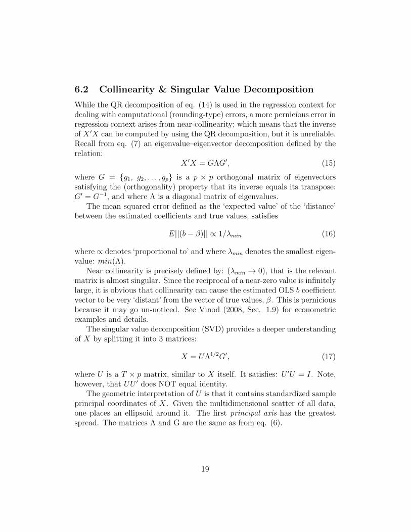
While the QR decomposition of eq. (14) is used in the regression context fordealing with computational (rounding-type) errors, a more pernicious error inregression context arises from near-collinearity; which means that the inverseof X ′X can be computed by using the QR decomposition, but it is unreliable.Recall from eq. (7) an eigenvalue–eigenvector decomposition defined by therelation:

X ′X = GΛG′, (15)

where G = g1, g2, . . . , gp is a p × p orthogonal matrix of eigenvectorssatisfying the (orthogonality) property that its inverse equals its transpose:G′ = G−1, and where Λ is a diagonal matrix of eigenvalues.

The mean squared error defined as the ‘expected value’ of the ‘distance’between the estimated coefficients and true values, satisfies

E||(b− β)|| ∝ 1/λmin (16)

where ∝ denotes ‘proportional to’ and where λmin denotes the smallest eigen-value: min(Λ).

Near collinearity is precisely defined by: (λmin → 0), that is the relevantmatrix is almost singular. Since the reciprocal of a near-zero value is infinitelylarge, it is obvious that collinearity can cause the estimated OLS b coefficientvector to be very ‘distant’ from the vector of true values, β. This is perniciousbecause it may go un-noticed. See Vinod (2008, Sec. 1.9) for econometricexamples and details.

The singular value decomposition (SVD) provides a deeper understandingof X by splitting it into 3 matrices:

X = UΛ1/2G′, (17)

where U is a T × p matrix, similar to X itself. It satisfies: U ′U = I. Note,however, that UU ′ does NOT equal identity.

The geometric interpretation of U is that it contains standardized sampleprincipal coordinates of X. Given the multidimensional scatter of all data,one places an ellipsoid around it. The first principal axis has the greatestspread. The matrices Λ and G are the same as from eq. (6).

19

PCR and SVD

Substituting SVD in eq. (9) we have:

y = Xβ + ε = UΛ1/2G′β + ε = UΛ1/2γ + ε, (18)

where we have used notation γ for G′β. The OLS estimate of γ is c = G′b,where the vector c has as many rows (components) as b.

In Principal Components Regression (PCR), some components of c aresimply deleted (weight = 0). Thus, the key decisions in using PCR are todecide how many components to delete and which one(s) to delete. Vinod(2008) explains why one should not delete principal components (eigenvec-tors) willy-nilly, but focus on deleting the relatively ‘unreliably estimated’components having high sampling variances. These are precisely the compo-nents associated with smallest eigenvalues or in order of preference set by:cp, cp−1, cp−2.

Ridge Regression

Ridge estimator represents a family of estimators parameterized by the bi-asing parameter k > 0. It can be recommended as a tool to solve near-collinearity. The ridge estimator and the corresponding variance–covariancematrix are:

bk = (X ′X + kI)−1X ′y, V (bk) = σ2(X ′X + kI)−1X ′X(X ′X + kI)−1.

(19)

A large number of choices of k ∈ [0,∞) are possible. Hoerl and Kennardproved that some k exists which will reduce MSE(b), the mean squarederror of the OLS estimator b. All choices lead to shrinkage of |b| by a form ofdown-weighting of the trailing components c = G′b associated with smallereigenvalues. See Vinod (2008) for details and R tools for choosing the biasingparameter k.

6.3 Heteroscedastic and Autocorrelated Errors

If regression errors ε have non-constant variances they are said to have het-eroscedasticity. Sometimes a researcher may not want to correct for thisproblem by using generalized least squares (GLS) which changes the model.

20

Then, all one can do is to test whether the presence of this problem makesregression coefficients statistically insignificant.

The usual variance-covariance matrix of of regression coefficients usedfor testing the hypothesis that any component of β equals zero is given bycov(b) = s2(X ′X)−1, where s2 is the residual variance. Prof. Hal White aneconometrician, and others have proposed to replace it by

vcovHC(b) = s2(X ′X)−1X ′ΩX (X ′X)−1, (20)

where Ω is some known function representing the assumed pattern of chang-ing variances. This is easily implemented in R by using the ‘vcovHC’ functionin the R package ‘sandwich’ by Zeileis (2004), who also provides examples.

The three matrices in equation (20) have two outside matrices identical.Zeileis (2004) calls them ‘bread’, ‘meat’ and ‘bread’ matrices. Statisticiansworking in robust estimators call them a Huber sandwich. Similar matricesarise in several estimation problems, including when regression errors haveautocorrelation. Heteroskedasticity and autocorrelation consistent (HAC)estimation of variance covariance matrix is given by his R function ‘vcovHAC’with similar syntax. If one wants to go beyond testing, Vinod (2010) providesnew general approaches and R software tools to simultaneously correct forboth of these problems, available at: http://www.fordham.edu/economics/vinod/autohetero.txt. This completes our discussion of matrix algebra Rsoftware tools used in the context of the regression model.

7 Correlation Matrices and Generalizations

Statisticians have long ago developed alternative standardization procedureswith desirable properties by extending eq. (2) to p vectors to handle multi-variate situations. The correlation matrix rij is a multivariate descriptivestatistics between two or more variables which is free from units of measure-ment. That is, it is invariant under any linear transformation.

Computation of the correlation matrix is accomplished by the command‘cor’ as:

ca=cor(A);ca

It is illustrated for our selected variables as:

21

mpg disp hp

mpg 1.0000000 -0.8475514 -0.7761684

disp -0.8475514 1.0000000 0.7909486

hp -0.7761684 0.7909486 1.0000000

Note that the correlation matrix is symmetric, rij = rji, because it measuresonly a linear dependence between the pairs of variables. The R function‘cor.test’ allows formal testing of the null hypothesis that the populationcorrelation is zero against various alternatives. I prefer the ‘rcorr’ functionof the ‘Hmisc’ package over ‘cor’ because ‘rcorr’ reports three matrices: (i)Pearson or Spearman correlation matrix with pairwise deletion of missingdata, (ii) The largest number of data points available for each pair, and (iii)Matrix of p-values.

Bounds on the cross correlation

If one knows the correlations r1=r(X,Y) and r2=r(X,Z), is it possible to writebounds for r3=r(Y,Z). Mr. Arthur Charpentier has posted a solution to thisproblem in terms of the following R function:

corrminmax=function(r1,r2,r3)

h=function(r3)

R=matrix(c(1,r1,r2,r1,1,r3,r2,r3,1),3,3)

return(min(eigen(R)$values)>0)

vc=seq(-1,+1,length=1e4+1)

vr=Vectorize(h)(vc)

indx=which(vr==TRUE)

return(vc[range(indx)])

We illustrate the use of this function for our cars data. We let r1 = r(mpg,disp), r2=r(mpg, hp) and r3=r(disp, hp). The function provides bounds onr3.

ca=cor(A)

corrminmax(ca[2,1], ca[3,1], ca[3,2])

Even though r1 and r2 are negative, the R function bounds correctly statethat r3 must be positive. The function ‘corrminmax’ returns the min andmax limits, or bounds on the third correlation coefficient r2 as:

22

#min r3, max r3

[1] 0.3234 0.9924

Now we turn to graphics for correlation matrices. In our illustration, theR object ‘ca’ contains the correlation matrix for A. There are several toolsfor plotting them available in R. We illustrate the code of few but omit alloutputs to save space.

#Need ca containing correlation matrix in R memory

require(sjPlot)

sj1=sjp.corr(ca)

sj1$df #data frame with correlations ordered by col. 1

require(psych)

cor.plot(ca)

7.1 New Asymmetric Generalized Correlation Matrix

Zheng et al. (2012) have recently developed generalized measures of corre-lation (GMC) by using Nadaraya-Watson nonparametric Kernel regressionsdesigned to overcome the linearity assumption of Pearson’s standard corre-lations, ρX,Y . Vinod (2013) developed a weak but potentially useful “kernel-causality” defined by using computer intensive data-driven kernel-based con-ditional densities: f(Y |X) and f(X|Y ). He defines δ = GMC(X|Y ) −GMC(Y |X). When δ < 0 we know from the properties of GMCs that Xbetter predicts Y than vice versa.

Using better prediction as an indicator of causation (by analogy withGranger causality) I define that “X kernel causes Y ” if δ < 0. The qualifier“kernel” in kernel causality should remind us that this causality is subject tofallacies, such as when the models are misspecified.

Ordinary correlations among p variables implies a symmetric p× p corre-lation matrix, where positive correlation means the two variables move in thesame direction. Since the GMC’s are always positive, they lose important in-formation regarding the direction of the relation. Hence, let us consider newgeneralized correlation coefficients ρ∗(Y |X) based on signed square roots ofthe GMC’s. We simply assign the sign of the simple correlation to that ofthe generalized one by defining a sign function, sign(ρXY ), equaling −1 if(ρXY < 0), and 1 if (ρXY ≥ 0).

23

Now the off-diagonal elements of our new correlation matrix are:

ρ∗(Y |X) = sign(ρXY)√

[GMC(Y|X)], (21)

Unlike the usual correlation matrix, this one is not symmetric. That is,ρ∗(Y |X) 6= ρ∗(X|Y ). When we have p variables, letting i, j = 1, 2, . . . p,the (i, j) location of the p × p matrix of generalized correlation coefficients(in population) contains ρ∗(Xi|Xj) = ρ∗ij, where the row variable Xi is the“effect” and the column variable Xj is the predictor or the “cause.” The p×pmatrix of generalized sample correlation coefficients is denoted as: r∗ij.

Let us consider a larger set of six ratio scale variables from the cars data.The following R code selects them, computes the matrix of simple correlationsand plots them is a color scheme to show ellipses as well as numbers usingthe R package ‘corrplot‘ by Wei (2013).

In the following code the object ‘ca’ contains the correlation matrix.

names(mtcars)

attach(mtcars)

mtx=cbind(mpg, disp, hp, drat, wt, qsec)

ca=cor(mtx)

require(corrplot)

corrplot.mixed(ca, upper="number", lower="ellipse")

These correlations (subject to the strong assumption of a linear relation)range from a high of 0.89 for ‘disp’ and ‘wt’ to a low of 0.091 between ‘qsec’and ‘drat.’ Figure 2 plots these symmetric correlations with color coding. Wedisplay rij numbers above the diagonal. Instead of reporting the symmet-ric numbers below the the diagonal, the command ‘corrplot.mixed’ displaysappropriate ellipses representing rij numbers below the diagonal, where neg-atively sloped ellipses indicate negative correlations.

24

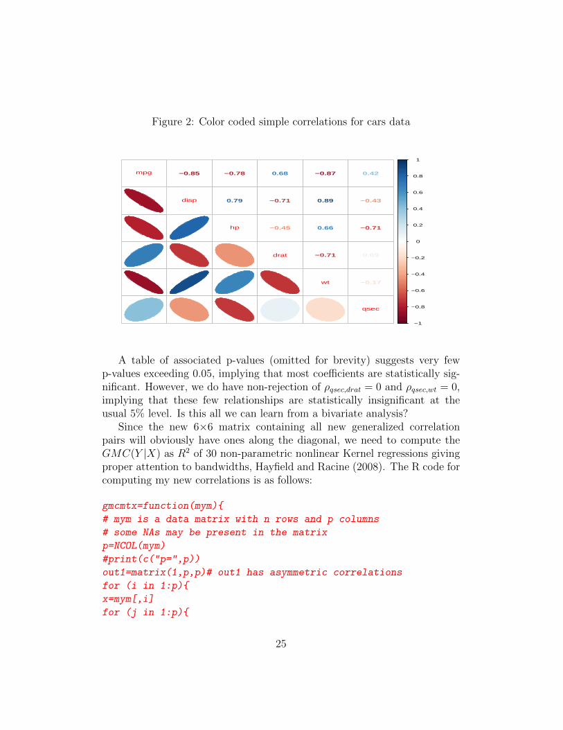
Figure 2: Color coded simple correlations for cars data

1 −0.85

1

−0.78

0.79

1

0.68

−0.71

−0.45

1

−0.87

0.89

0.66

−0.71

1

0.42

−0.43

−0.71

0.09

−0.17

1

−1

−0.8

−0.6

−0.4

−0.2

0

0.2

0.4

0.6

0.8

1

mpg

disp

hp

drat

wt

qsec

A table of associated p-values (omitted for brevity) suggests very fewp-values exceeding 0.05, implying that most coefficients are statistically sig-nificant. However, we do have non-rejection of ρqsec,drat = 0 and ρqsec,wt = 0,implying that these few relationships are statistically insignificant at theusual 5% level. Is this all we can learn from a bivariate analysis?

Since the new 6×6 matrix containing all new generalized correlationpairs will obviously have ones along the diagonal, we need to compute theGMC(Y |X) as R2 of 30 non-parametric nonlinear Kernel regressions givingproper attention to bandwidths, Hayfield and Racine (2008). The R code forcomputing my new correlations is as follows:

gmcmtx=function(mym)

# mym is a data matrix with n rows and p columns

# some NAs may be present in the matrix

p=NCOL(mym)

#print(c("p=",p))

out1=matrix(1,p,p)# out1 has asymmetric correlations

for (i in 1:p)

x=mym[,i]

for (j in 1:p)

25

if (j>i) y=mym[,j]

ava.x=which(!is.na(x))#ava means available

ava.y=which(!is.na(y))#ava means non-missing

ava.both=intersect(ava.x,ava.y)

newx=x[ava.both]#delete NAs from x

newy=y[ava.both]#delete NAs from y

c1=cor(newx,newy)

sig=sign(c1) #get sign of r(x,y)

#bandwidths for non parametric regressions

bw=npregbw(formula=newx~newy,tol=0.1, ftol=0.1)

mod.1=npreg(bws=bw, gradients=FALSE, residuals=TRUE)

corxy= sqrt(mod.1$R2)*sig #sign times r*(x|y)

out1[i,j]=corxy # r(i,j) has xi given xj as the cause

bw2=npregbw(formula=newy~newx,tol=0.1, ftol=0.1)

mod.2=npreg(bws=bw2, gradients=FALSE, residuals=TRUE)

coryx= sqrt(mod.2$R2)*sig #sign times r*(y|x)

out1[j,i]=coryx

#end i loop

#end j loop

#endif

return(out1)

We need to supply this function with the data matrix of six variables andthen plot them by the following code.

require(np)

cg=gmcmtx(mtx)

colnames(cg)=colnames(mtx)

rownames(cg)=colnames(mtx)

require(xtable)

print(xtable(cg, digits=3))

The interpretation of new generalized correlations is straightforward. If|r∗ij| > |r∗ji|, it is more likely that the row variable Xi is the “effect” and thecolumn variable Xj is the “cause”, or at least Xj is the better predictor ofXi, than vice versa. For example, letting i = 1, j = 2 the entries in Table 2show 0.951 = |r∗12| > |r∗21| = 0.894. This suggests that ‘disp’ better predicts‘mpg’ than vice versa.

26

Table 2: Table of asymmetric generalized correlations among car variables

mpg disp hp drat wt qsecmpg 1.000 -0.951 -0.938 0.685 -0.916 0.738disp -0.894 1.000 0.931 -0.770 0.901 -0.761

hp -0.853 0.817 1.000 -0.554 0.693 -0.927drat 0.688 -0.946 -0.744 1.000 -0.750 0.549

wt -0.917 0.968 0.920 -0.730 1.000 -0.772qsec 0.751 -0.609 -0.754 0.230 -0.188 1.000

Now the following code creates a color coded asymmetric plot by callingthe ‘corrplot’ function as follows.

require(corrplot)

corrplot(cg, method="ellipse")

Figure 3 plots our new generalized asymmetric correlation coefficientsdefined in eq. (21) with color coding similar to Figure 2.

Figure 3: Color coded generalized asymmetric correlations for cars data

−1

−0.8

−0.6

−0.4

−0.2

0

0.2

0.4

0.6

0.8

1

mpg

disp

hp drat

wt qsec

mpg

disp

hp

drat

wt

qsec

Finally we claim that asymmetric correlations in Table 2 contain usefulcausation information in their asymmetry itself. We have noted that when

27

the asymmetry satisfies |r∗ij| > |r∗ji|, the variable Xj is more likely to be causethan the variable Xi. Hence the new table and Figure 3 represent usefulsupplements to the traditional table and Figure 2. This has applications inall sciences including newer exploratory techniques using ‘Big Data.’

8 Matrices for Population Dynamics

Births, deaths, and migrations affect the population dynamics of variouscreatures. Demographers have long known that age, size, or life-history ofindividuals in any population influences the growth, survival and reproduc-tion of the population.

Let nt denote a vector of populations at time t for various age, size, orstage categories. Its transition is given by

nt+1 = Ant, where A = T + F (22)

where transitions matrix T represents growth and survival and where F rep-resents fertilities or transitions due to reproduction. A powerful R package‘popbio’ by Stubben and Milligan (2007) is available for studying varioustransition matrices and models. It offers a basic function ‘pop.projection’for projection through equation (22). The demographers have developed so-phisticated methods for reproductive value, damping ratio, sensitivity, andelasticity using eigenvalues of the matrix A, accomplished by the command‘eigen.analysis(A).’ The function ‘stoch.projection’ can be used to simulatestochastic population growth.

This package is intended for R novices and includes a command ‘demo’which offers an overview.

require(popbio)

demo("fillmore")

years=unique(aq.trans$year)

sv<-table(aq.trans$stage, aq.trans$year)

addmargins(sv)

round(apply(sv, 1, mean),0)

stage.vector.plot(sv[-1,], prop=FALSE, col=rainbow(4),

ylab = "Total number of plants",

main = "Fillmore Canyon stage vectors")

28

Census data is in the form of transition data listing stages and fates fromAquilegia chrysantha in Fillmore Canyon, Organ Mountains, New Mexico,1996-2003. One constructs and analyzes population projection matrices.Typical data are not available as matrices of the recurrence relation (22).The package ‘popbio’ converts such data into usable forms.

head2(aq.trans)

plot year plant stage leaf rose fruits fate rose2

1 903 1996 1 small 0 0 0 small NA

2 903 1996 2 flower NA NA 1 large NA

3 903 1996 3 small 0 0 0 large NA

. . . . . . . . . .

1637 930 2003 86 small 6 1 0 flower 1

addmargins(sv)

1996 1997 1998 1999 2000 2001 2002 2003 Sum

seed 0 0 0 0 0 0 0 0 0

recruit 12 287 186 76 5 5 0 3 574

small 134 75 60 84 58 31 13 6 461

large 17 68 41 57 59 58 16 4 320

flower 62 6 80 74 52 8 0 0 282

Sum 225 436 367 291 174 102 29 13 1637

## mean stage vector

round(apply(sv, 1, mean),0)

seed recruit small large flower

0 72 58 40 35

Figure 4 plots the graphics produced by the code. The demo also providescode for sensitivity and elasticity matrices and many more figures.

$sensitivities

seed recruit small large flower

seed 0.01112 0.0000 0.0000 0.0000 0.0002123

recruit 1.60604 0.0000 0.0000 0.0000 0.0306479

small 0.00000 0.2844 0.2122 0.2048 0.1466064

large 0.00000 0.0000 0.3793 0.3660 0.2619686

flower 0.00000 0.6814 0.5084 0.4906 0.3511985

$elasticities

29

seed recruit small large flower

seed 0.002025 0.0000000 0.00000 0.00000 0.009098

recruit 0.009098 0.0000000 0.00000 0.00000 0.050362

small 0.000000 0.0587038 0.10262 0.03191 0.019009

large 0.000000 0.0000000 0.05277 0.17393 0.139268

flower 0.000000 0.0007563 0.05686 0.16013 0.133461

$repro.value

seed recruit small large flower

1.0 144.4 690.7 1234.2 1654.5

We have given an overview of recent R resources for matrices arising in demo-graphics. The interested readers should consult further references by Stubbenand Milligan (2007).

Figure 4: Population stages for Fillmore Canyon

1996 1997 1998 1999 2000 2001 2002 2003

050

100

150

200

250

Fillmore Canyon stage vectors

Years

Total

numb

er of

plants

recruit small large flower

9 Multivariate Components Analysis

While correlation analysis studies joint dependence of two variables at atime, there is an obvious interest in extending it to several variables. Partialcorrelations study the relation between (X, Y ), upon removing the effect

30

of a third variable Z. Multivariate analysis can involve a study of jointdependence of one set of variables on another set of variables.

9.1 Projection Matrix: Generalized CanonicalCorrelations

R function ‘cancor’ readily computes the canonical correlations between twodata matrices. An application to estimation of joint production function(between wool and mutton on the output side and capital and labor on theinput side) is discussed in Vinod (2008), section 5.2. A generalized canonicalcorrelation analysis is available under dependency modeling toolkit of the Rpackage ‘dmt’ by Lahti and Huovilainen (2013).

We illustrate it for the cars data with two sets of three variables in thefollowing R code. An underlying latent variable model assumes that the twodata sets, mtx1 and mtx2 can be decomposed in shared and data set specificcomponents. In our artificial example from cars data, this assumption islikely to be invalid.

attach(mtcars); require(dmt)

mtx1=cbind(mpg,disp,hp)#first set of 3 variables

mtx2=cbind(drat,wt,qsec)

rc=regCCA(list(mtx1,mtx2))

print(head(rc$proj,3), digits=3)

matplot(rc$proj, typ="l", main="Projection matrix

of (mpg, disp, hp) against (drat, wt, qsec)")

drCCAcombine(list(mtx1,mtx2)) #dimension reduction

sharedVar(list(mtx1,mtx2),rc,3)#shared variation retained

fit.dependency.model(mtx1,mtx2) #Bayesian with exponential priors

The detailed output is suppressed for brevity. We report only the first fewlines and a plot of the six sets of components of the projection matrix.

print(head(rc$proj,3), digits=3)

[,1] [,2] [,3] [,4] [,5] [,6]

[1,] -0.508 -0.498 -0.407 0.641 0.977 -0.0999

[2,] -0.444 -0.259 -0.688 0.360 0.738 -0.1635

[3,] -1.221 0.177 -0.417 0.915 0.120 0.0801

31

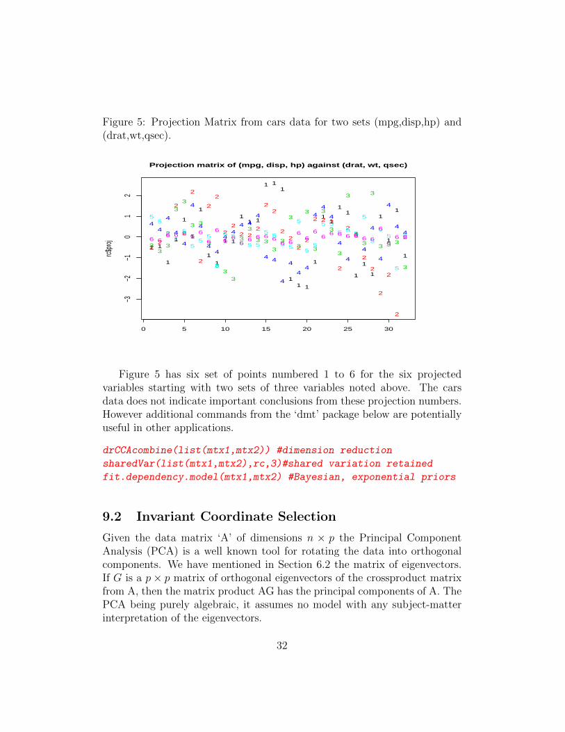
Figure 5: Projection Matrix from cars data for two sets (mpg,disp,hp) and(drat,wt,qsec).

1 1

1

1

1

1

1

1

1

1 1

11 1

1 11

11 1

1

11

11

1

1

1

1

1

1

1

0 5 10 15 20 25 30

−3−2

−10

12

Projection matrix of (mpg, disp, hp) against (drat, wt, qsec)

rc$pr

oj

22

2

2

2

2

2

2

2

22

2 22

22

22

22

2 2 2

2

22

2

2

2

2

2

2

33

3

3

3

3 3

3

33

3

3

3

3 3

3

3

3

3

3

3

3

3

3

3

3

3

3

3 3 3

3

44

4

4

4

4

4

44

44

4 44

4 4

4

4

44

4

4

4

4

4

4

4

4

4

4

44

55

55

5

55

5

5

5 55 5 5

55

5 5

5

55

5 5

5 55

5

5

55

5

56 6

6 6 6 66

6

6

66

66 6 6 6

6 6

66

66

6 6 6 6 6 6

6

66 6

Figure 5 has six set of points numbered 1 to 6 for the six projectedvariables starting with two sets of three variables noted above. The carsdata does not indicate important conclusions from these projection numbers.However additional commands from the ‘dmt’ package below are potentiallyuseful in other applications.

drCCAcombine(list(mtx1,mtx2)) #dimension reduction

sharedVar(list(mtx1,mtx2),rc,3)#shared variation retained

fit.dependency.model(mtx1,mtx2) #Bayesian, exponential priors

9.2 Invariant Coordinate Selection

Given the data matrix ‘A’ of dimensions n × p the Principal ComponentAnalysis (PCA) is a well known tool for rotating the data into orthogonalcomponents. We have mentioned in Section 6.2 the matrix of eigenvectors.If G is a p× p matrix of orthogonal eigenvectors of the crossproduct matrixfrom A, then the matrix product AG has the principal components of A. ThePCA being purely algebraic, it assumes no model with any subject-matterinterpretation of the eigenvectors.

32

The R package ‘ICS,’ Nordhausen et al. (2008), allows deeper multivari-ate analyses for Invariant Coordinate Selection (ICS) allowing interpretationof algebraic constructs. This is a two-step process. The first step standard-izes the data wrt a covariance matrix, say S1. The second step performsa PCA transformation using a different covariance-type matrix S2. If B issome matrix which simultaneously diagonalizes both S1 and S2, then postmultiplying the data matrix by this B gives the ICS transform. The packageauthors cite some 12 choices of S2 available in various R packages.

The ICS transform uses two covariance-type scatter matrices. S1 is oftenthe usual covariance matrix used in standardization of data. The secondcovariance S2 is defined differently from S1. The default for S2 is a robustestimate based on fourth order moments. It is used to find a rotation ofthe data obtained from a PCA of the standardized data. The new coordi-nate system is invariant (up to a sign change) under affine transformationsmentioned above.

The ‘ics’ function involves two covariance-type matrices, S1 and S2 andyields the invariant coordinates.

screeplot(princomp(A))#plot omitted for brevity

attach(mtcars);A=cbind(mpg,disp,hp)

require(ICS)

icsA=ics(A); icsA

The ‘ics’ function also gives a generalized measure of the kurtosis computedby a ratio of quadratic forms and ‘Unmixing’ matrix explained in Nordhausenet al. (2008). The output of the above code is next.

$gKurt

[1] 1.7133 0.8739 0.6679

$UnMix

[,1] [,2] [,3]

[1,] 0.04161 -0.008423 0.024608

[2,] 0.26644 0.003913 0.005282

[3,] -0.19138 -0.013723 -0.001489

The unmixing matrix allows one to get independent components by sim-ply post-multiplying rows of data by this matrix. For our data un-mixeddata matrix is given by the commands:

33

Apost=A %*% icsA@UnMix

matplot(Apost)

The first line of the code shows post multiplication of A by the unmixingmatrix, where is accessed with the ‘at’ (@) symbol–not the usual $ symbol.The plot is omitted for brevity, but shows that unmixing is successful. Thetwo covariance-type matrices S1 and S2 are accessed by the code below.

icsA@S1 #print basic covariance matrix

icsA@S2 #cov from fourth order moments.

icc=as.matrix(ics.components(icsA))

head(icc,3) #initial coordinate components

matplot(icc, main="Invariant Coordinates, cars data")

Now we report the S1, S2 matrices and initial independent components.

icsA@S1 #print basic covariance matrix

mpg disp hp

mpg 36.32 -633.1 -320.7

disp -633.10 15360.8 6721.2

hp -320.73 6721.2 4700.9

icsA@S2 #cov from fourth order moments.

mpg disp hp

mpg 30.49 -497.3 -292.1

disp -497.35 11036.1 5266.4

hp -292.10 5266.4 5362.6

icc=as.matrix(ics.components(icsA))

head(icc,3) #initial coordinates

IC.1 IC.2 IC.3

[1,] 2.233 6.802 -6.378

[2,] 2.233 6.802 -6.378

[3,] 2.328 6.989 -5.984

The separation of coordinates obtained by the ICS package is seen in Figure6. A related package called ‘ICSNP’ allows nonparametric (distribution-free)testing.

34

Figure 6: Invariant coordinates for A from cars data showing visible separa-tion.

1 1 11

11

1

11 1 1

1 1 1

1 11 1 1

1 11 1

1

1 1 11

1 1

1

1

0 5 10 15 20 25 30

−10

−50

510

Invariant Coordinates, cars data

icc

2 2 2 2 2

2 22 2

2 2 2 22 2 2

2

22

2

22 2 2

2 2 2

2

2 2 2 2

3 3 3

33

3

3

3 3 3 3

3 3 3

3 33

33

3

3

3 3 3

3

3 33

3

3

3

3

require(ICSNP)

rank.ctest(icc, scores="normal")

The output of above commands is

Marginal One Sample Normal Scores Test

data: icc

T = 27.5234, df = 3, p-value = 4.573e-06

alternative hypothesis: true location is not equal to c(0,0,0)

Not surprisingly, the null of zero means is rejected. These tools havealso been applied to signal processing or image separation. The authors ofthe package have given simulation examples showing that their multivariatenonparametric distribution-free testing works well.

10 Sparse Matrices

There are many applications where the matrices involved have have a largenumber of entries which are zero. This section reviews some R tools for effi-ciently handling them without burdening the R memory. Examples include

35

indicator variable, design matrices of smoothing splines, fixed effects models,etc., as given in Koenker and Ng (2003).

We construct an artificial sparse matrix

set.seed(345)

a=sample(1:100)[1:(5*4)];a

a[a>25]=0;a

A=matrix(a,5,4);A

In this code the line ‘a[a>25]=0’ sets several elements to zero before con-structing the matrix A of dimension 5× 4 from the 20 numbers in ‘a,’ goingcolumn-wise.

a=sample(1:100)[1:(5*4)];a

[1] 22 28 39 64 42 77 37 78 44 9 24 85 16 55 83 8 80 21 84 71

a[a>25]=0;a

[1] 22 0 0 0 0 0 0 0 0 9 24 0 16 0 0 8 0 21 0 0

A=matrix(a,5,4);A

[,1] [,2] [,3] [,4]

[1,] 22 0 24 8

[2,] 0 0 0 0

[3,] 0 0 16 21

[4,] 0 0 0 0

[5,] 0 9 0 0

Now let us use the function ‘as.matrix.csr’ of the package ‘SparseM’ to storeit in a compressed sparse row (csr) format.

require(SparseM)

amc=as.matrix.csr(A)

myx=rbind(amc@ra,amc@ja)

image(myx, main="Visual location of nonzero entries")

rownames(myx)=c("ra","ja");myx

amc@ia

The csr format has four slots. The slot ‘ra’ lists all nonzero values. Thesecond slot ‘ja’ lists the column indexes of the nonzero elements stored in‘ra.’

rownames(myx)=c("ra","ja");myx

[,1] [,2] [,3] [,4] [,5] [,6]

36

ra 22 24 8 16 21 9

ja 1 3 4 3 4 2

amc@ia

[1] 1 4 4 6 6 7

The third slot ‘ia’ is the heart of compressing a vector of elements for eco-nomical storage. Unfortunately, its official description is hard to understand.I will give a new description below. We focus on non-zero locations only andwrite an ad hoc R function called ‘fc’ to compute their count.

fc=function(x)length(x[x!=0])

m=apply(A,1,fc);m

The output of the above code correctly counts the number of non-zero ele-ments in each row as m=(3, 0, 2, 0, 1).

m=apply(A,1,fc);m

[1] 3 0 2 0 1

Now define m2 as one obtained by padding a one at the start, or (1,m) vector.Then the compressed vector ‘ia’ is the cumulative sum of m2 integers.

m2=c(1,m);m2

cumsum(m2)

The output is

m2=c(1,m);m2

[1] 1 3 0 2 0 1

cumsum(m2)

[1] 1 4 4 6 6 7

Verify that the output of the command ‘as.matrix.csr(A)’ agrees with ‘cum-sum(m2)’. Since the compressed sparse row (csr) method applies to anypattern of non-zeros in A, it is commonly used for dealing with generalsparse matrices. Matrix algebra for patterned matrices is discussed in Vinod(2011)[ch.16].

The R package ‘SparseM’ provides useful functions for various matrixoperations including coercion and linear equation solving. Linear regressionwith sparse data is implemented by generalizing the ‘lm’ function to achievesimilar functionality with ‘slm, print.summary.slm’ functions. Of course, the

37

implementation uses more suitable Cholesky rather than QR methods in thesparse data context.

A regression example has a sparse matrix of regressors of dimension 1850×712.

require(SparseM);data(lsq)

X <- model.matrix(lsq) #extract th

y <- model.response(lsq) # extract the rhs

X1 <- as.matrix(X)

reg1=slm(y~X1-1)

su1=summary(reg1)

head(su1$coef)

su1$adj.r.squared

The command ‘image(X,main="Visual location of nonzero entries")’creates a graph displaying dots at all locations of non-zero entries in the largematrix seen in Figure 7.

Note that the ‘slm’ function is similar to the ‘lm’. We report below a fewlines from the 712 regression coefficients computed at great speed and theadjusted R2.

head(su1$coef)

Estimate Std. Error t value Pr(>|t|)

[1,] 823.3613 0.1274477 6460.3857 0

[2,] 340.1156 0.1711477 1987.2631 0

[3,] 472.9760 0.1379109 3429.5758 0

[4,] 349.3175 0.1743084 2004.0201 0

[5,] 187.5595 0.2099702 893.2673 0

[6,] 159.0518 0.2201477 722.4776 0

tail(su1$coef)

Estimate Std. Error t value Pr(>|t|)

[707,] -2.0801136 0.13312708 -15.625022 0.00000000

[708,] -6.4395314 0.14294089 -45.050310 0.00000000

[709,] -0.1259875 0.05397642 -2.334121 0.01976273

[710,] -0.1191570 0.10272585 -1.159952 0.24631169

[711,] -2.0601158 0.05816518 -35.418367 0.00000000

[712,] -7.8488311 0.18087842 -43.392856 0.00000000

su1$adj.r.squared #$

[1] 0.9999999

38

Figure 7: The non-zero entries of a huge 1850× 712 sparse regressor matrixshown as dots.

Visual location of nonzero entries

column

row

200 400 600

1500

1000

500

The R package ‘Matrix’ also has several functions for sparse data. Ithas a great variety of sparse matrix operations and storage modes. Forexample, instead of ‘chol’, it offers a sparse matrix version called ‘Cholesky’.Considerable programming ingenuity is needed to work with sparse matrices.Our discussion can help an applied researcher who may not want to learnthose intricacies. Another worthy R package ‘spam’ uses available Fortranroutines for sparse matrices and Cholesky factorization, and extends them tosparse matrix algebra.

This chapter has reviewed several important topics from matrix algebrarelevant for Statistics and Economics. We have provided explicit R softwaretools for all topics discussed along with illustrative examples.

References

Gantmacher, F. R. (1959), The Theory of Matrices, vol. I and II, New York:Chelsea Publishing.

Hayfield, T. and Racine, J. S. (2008), “Nonparametric Econometrics: The

39

np Package,” Journal of Statistical Software, 27, 1–32, URL http://www.

jstatsoft.org/v27/i05/.

Henderson, H. V. and Velleman, P. F. (1981), “Building Multiple RegressionModels Interactively,” Biometrics, 37 (2), 391–411.

Koenker, R. and Ng, P. (2003), “SparseM: A Sparse Matrix Package for R,”Journal of Statistical Software, 8, 1–9, URL http://www.jstatsoft.org/

v08/i06.

Lahti, L. and Huovilainen, O.-P. (2013), dmt: Dependency Modeling Toolkit,r package version 0.8.20, URL http://CRAN.R-project.org/package=

dmt.

Nordhausen, K., Oja, H., and Tyler, D. E. (2008), “Tools for Exploring Multi-variate Data: The Package ICS,” Journal of Statistical Software, 28, 1–31,URL http://www.jstatsoft.org/v28/i06.

Rao, C. R. (1973), Linear Statistical Inference And Its Applications, NewYork: J. Wiley and Sons, 2nd ed.

Serfling, R. (2009), “Equivariance and Invariance Properties of Multivari-ate Quantile and Related Functions, and the Role of Standardization,”Tech. rep., University of Texas at Dallas, URL http://www.utdallas.

edu/~serfling/papers/Equivariance_November2009.pdf.

Stubben, C. J. and Milligan, B. G. (2007), “Estimating and Analyzing De-mographic Models Using the popbio Package in R,” Journal of StatisticalSoftware, 22, 1–23, URL http://www.jstatsoft.org/v22/i11.

Venables, W. N. and Ripley, B. D. (2002), Modern Applied Statistics withS, New York: Springer, 4th ed., ISBN 0-387-95457-0, URL http://www.

stats.ox.ac.uk/pub/MASS4.

Vinod, H. D. (1978), “Equivariance of ridge estimators through standardiza-tion: A note,” Communications in Statistics, A 7(12), 1159–1167.

— (2008), Hands-on Intermediate Econometrics Using R: Templates forExtending Dozens of Practical Examples, Hackensack, NJ: World Sci-entific, ISBN 10-981-281-885-5, URL http://www.worldscibooks.com/

economics/6895.html.

40

— (2010), “Superior Estimation and Inference Avoiding Heteroscedasticityand Flawed Pivots: R-example of Inflation Unemployment Trade-Off,” in“Advances in Social Science Research Using R,” , ed. Vinod, H. D., NewYork: Springer, pp. 39–63.

— (2011), Hands-on Matrix Algebra Using R: Active and Motivated Learningwith Applications, Hackensack, NJ: World Scientific, ISBN 978-981-4313-68-1, URL http://www.worldscibooks.com/mathematics/7814.html.

— (2013), “Generalized Correlation and Kernel Causality with Applicationsin Development Economics,” SSRN eLibrary, URL http://ssrn.com/

paper=2350592.

Wei, T. (2013), corrplot: Visualization of a correlation matrix, R packageversion 0.73, URL http://CRAN.R-project.org/package=corrplot.

Zeileis, A. (2004), “Econometric Computing with HC and HAC CovarianceMatrix Estimators,” Journal of Statistical Software, 11, 1–17, URL http:

//www.jstatsoft.org/v11/i10/.

Zheng, S., Shi, N.-Z., and Zhang, Z. (2012), “Generalized Measures of Corre-lation for Asymmetry, Nonlinearity, and Beyond,”Journal of the AmericanStatistical Association, 107, 1239–1252.

41