Embed Size (px)
Citation preview
Matrix Algebra and the Multivariate Normal Distribution
Generalized Linear Mixed Models
Lecture 2
September 2, 2015
GLMM Lecture 2: Matrix Algebra and MVN
Today’s Class
• Brief introduction to matrix algebra
• Multivariate normal distribution
• Additional lecture on Chapter 1 without slides
GLMM Lecture 2: Matrix Algebra and MVN 2
BRIEF PRIMER ON MATRIX ALGEBRA
For Reading and Deciphering Multivariate Distributions
GLMM Lecture 2: Matrix Algebra and MVN 3
Definitions
• We begin this section with some general definitions (from dictionary.com):
Matrix:
1. A rectangular array of numeric or algebraic quantities subject to mathematical operations
2. The substrate on or within which a fungus grows
Algebra:
1. A branch of mathematics in which symbols, usually letters of the alphabet, represent numbers or members of a specified set and are used to represent quantities and to express general relationships that hold for all members of the set
2. A set together with a pair of binary operations defined on the set. Usually, the set and the operations include an identity element, and the operations are commutative or associative
GLMM Lecture 2: Matrix Algebra and MVN 4
Why Learn Matrix Algebra
• Matrix algebra can seem very abstract from the purposes of this class (and statistics in general)
• Learning matrix algebra is important for: Understanding how statistical methods work
And when to use them (or not use them)
Understanding what statistical methods mean
Reading and writing results from new statistical methods
• Today’s class is the first lecture of learning the language of multivariate statistics and structural equation modeling
GLMM Lecture 2: Matrix Algebra and MVN 5
DATA EXAMPLE AND R
GLMM Lecture 2: Matrix Algebra and MVN 6
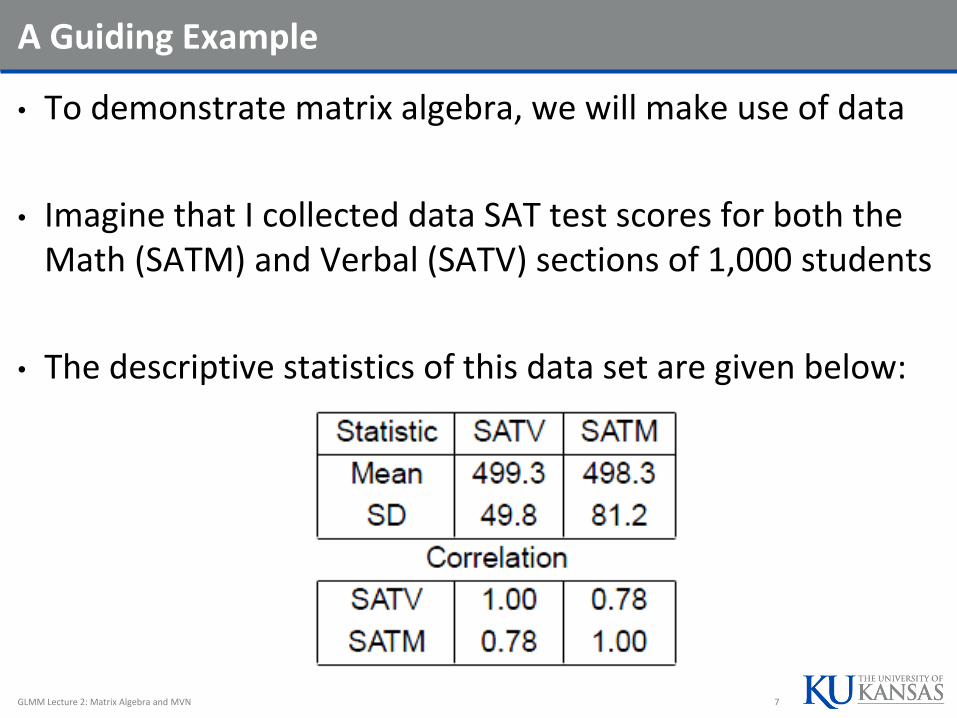
A Guiding Example
• To demonstrate matrix algebra, we will make use of data
• Imagine that I collected data SAT test scores for both the Math (SATM) and Verbal (SATV) sections of 1,000 students
• The descriptive statistics of this data set are given below:
GLMM Lecture 2: Matrix Algebra and MVN 7
DEFINITIONS OF MATRICES, VECTORS, AND SCALARS
GLMM Lecture 2: Matrix Algebra and MVN 8
Matrices
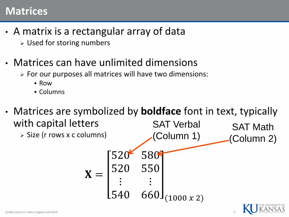
• A matrix is a rectangular array of data Used for storing numbers
• Matrices can have unlimited dimensions For our purposes all matrices will have two dimensions:
Row Columns
• Matrices are symbolized by boldface font in text, typically with capital letters
Size (r rows x c columns)
𝐗 =
520 580520 550⋮ ⋮540 660 (1000 𝑥 2)
GLMM Lecture 2: Matrix Algebra and MVN 9
SAT Verbal
(Column 1)SAT Math
(Column 2)
Vectors
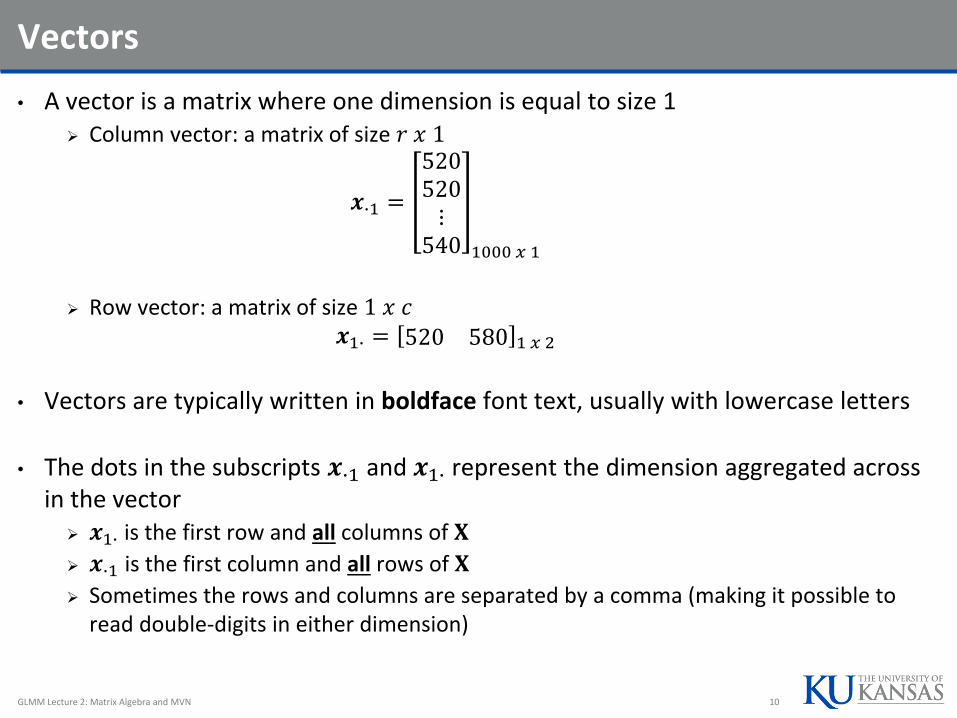
• A vector is a matrix where one dimension is equal to size 1 Column vector: a matrix of size 𝑟 𝑥 1
𝒙∙1 =
520520⋮540 1000 𝑥 1
Row vector: a matrix of size 1 𝑥 𝑐𝒙1∙ = 520 580 1 𝑥 2
• Vectors are typically written in boldface font text, usually with lowercase letters
• The dots in the subscripts 𝒙∙1 and 𝒙1∙ represent the dimension aggregated across in the vector
𝒙1∙ is the first row and all columns of 𝐗
𝒙∙1 is the first column and all rows of 𝐗
Sometimes the rows and columns are separated by a comma (making it possible to read double-digits in either dimension)
GLMM Lecture 2: Matrix Algebra and MVN 10
Matrix Elements
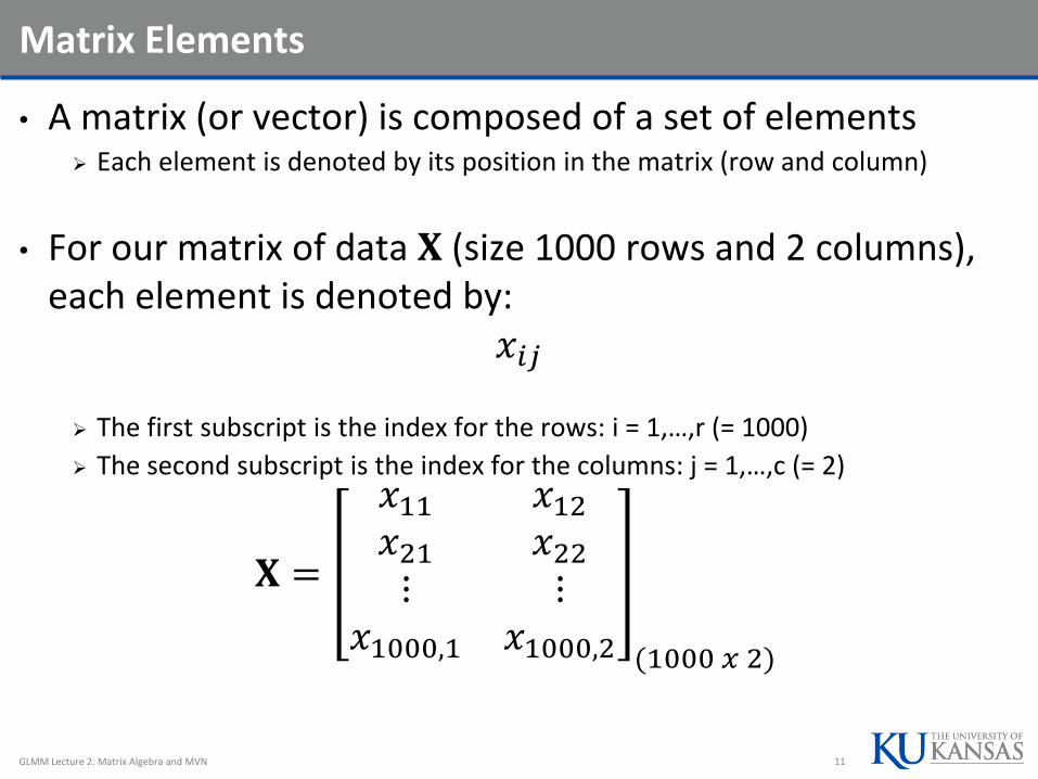
• A matrix (or vector) is composed of a set of elements Each element is denoted by its position in the matrix (row and column)
• For our matrix of data 𝐗 (size 1000 rows and 2 columns), each element is denoted by:
𝑥𝑖𝑗
The first subscript is the index for the rows: i = 1,…,r (= 1000)
The second subscript is the index for the columns: j = 1,…,c (= 2)
𝐗 =
𝑥11 𝑥12𝑥21 𝑥22⋮ ⋮𝑥1000,1 𝑥1000,2 (1000 𝑥 2)
GLMM Lecture 2: Matrix Algebra and MVN 11
Scalars
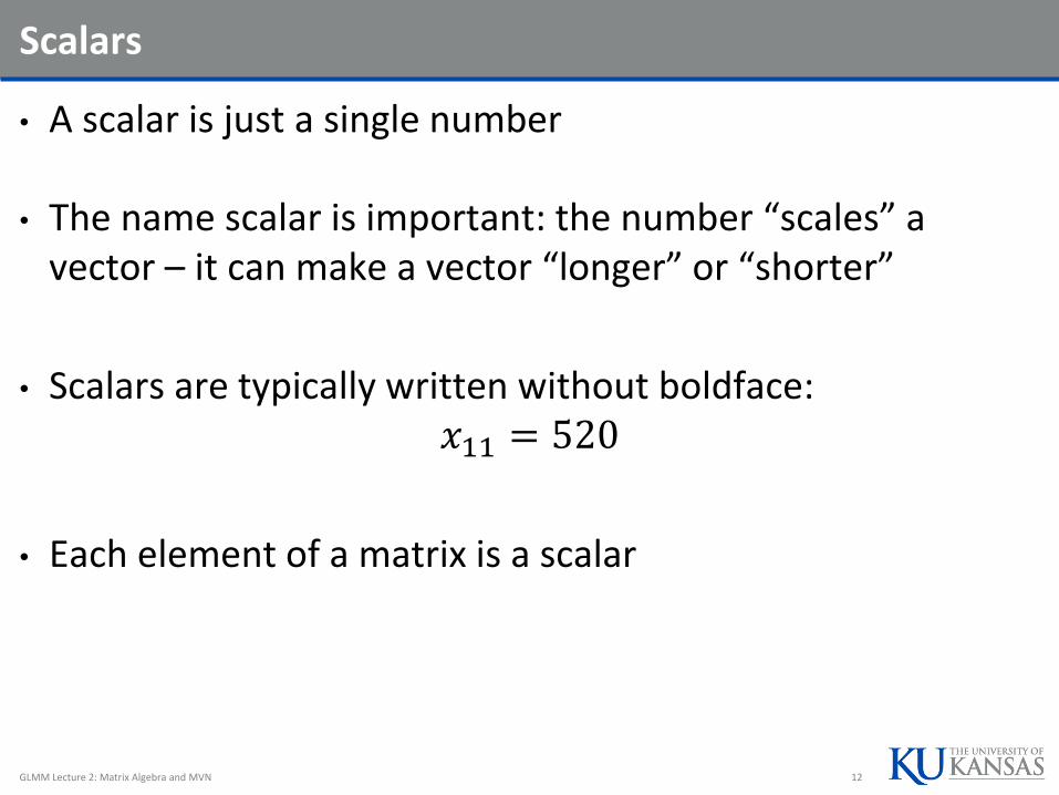
• A scalar is just a single number
• The name scalar is important: the number “scales” a vector – it can make a vector “longer” or “shorter”
• Scalars are typically written without boldface:𝑥11 = 520
• Each element of a matrix is a scalar
GLMM Lecture 2: Matrix Algebra and MVN 12
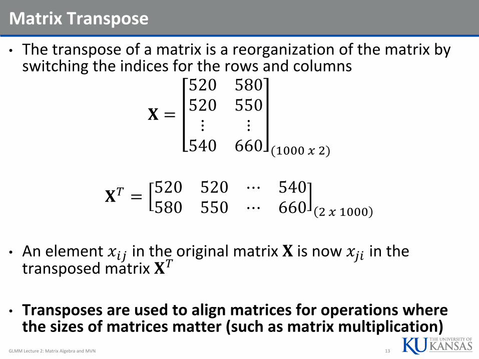
Matrix Transpose
• The transpose of a matrix is a reorganization of the matrix by switching the indices for the rows and columns
𝐗 =
520 580520 550⋮ ⋮540 660 (1000 𝑥 2)
𝐗𝑇 =520 520 ⋯ 540580 550 ⋯ 660 2 𝑥 1000
• An element 𝑥𝑖𝑗 in the original matrix 𝐗 is now 𝑥𝑗𝑖 in the transposed matrix 𝐗𝑇
• Transposes are used to align matrices for operations where the sizes of matrices matter (such as matrix multiplication)
GLMM Lecture 2: Matrix Algebra and MVN 13
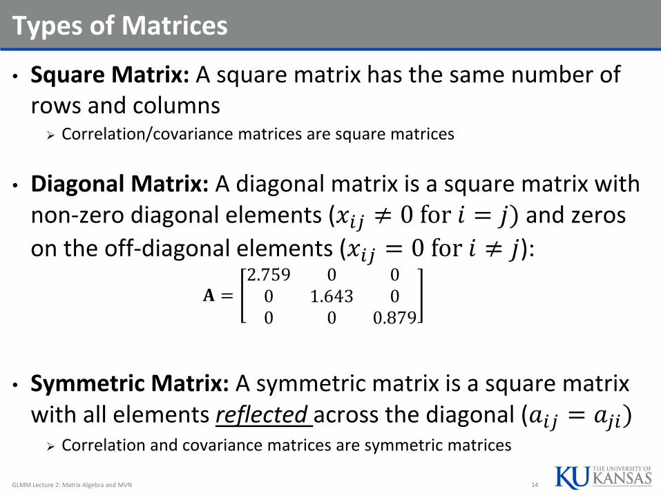
Types of Matrices
• Square Matrix: A square matrix has the same number of rows and columns
Correlation/covariance matrices are square matrices
• Diagonal Matrix: A diagonal matrix is a square matrix with non-zero diagonal elements (𝑥𝑖𝑗 ≠ 0 for 𝑖 = 𝑗) and zeros
on the off-diagonal elements (𝑥𝑖𝑗 = 0 for 𝑖 ≠ 𝑗):
𝐀 =2.759 0 00 1.643 00 0 0.879
• Symmetric Matrix: A symmetric matrix is a square matrix with all elements reflected across the diagonal (𝑎𝑖𝑗 = 𝑎𝑗𝑖)
Correlation and covariance matrices are symmetric matrices
GLMM Lecture 2: Matrix Algebra and MVN 14
MATRIX ALGEBRA
GLMM Lecture 2: Matrix Algebra and MVN 15
Matrices
• A matrix can be thought of as a collection of vectors Matrix operations are vector operations on steroids
• Matrix algebra defines a set of operations and entities on matrices
I will present a version meant to mirror your previous algebra experiences
• Definitions: Identity matrix Zero vector Ones vector
• Basic Operations: Addition Subtraction Multiplication “Division”
GLMM Lecture 2: Matrix Algebra and MVN 16
Matrix Addition and Subtraction
• Matrix addition and subtraction are much like vector addition/subtraction
• Rules: Matrices must be the same size (rows and columns)
• Method: The new matrix is constructed of element-by-element addition/subtraction of
the previous matrices
• Order: The order of the matrices (pre- and post-) does not matter
GLMM Lecture 2: Matrix Algebra and MVN 17
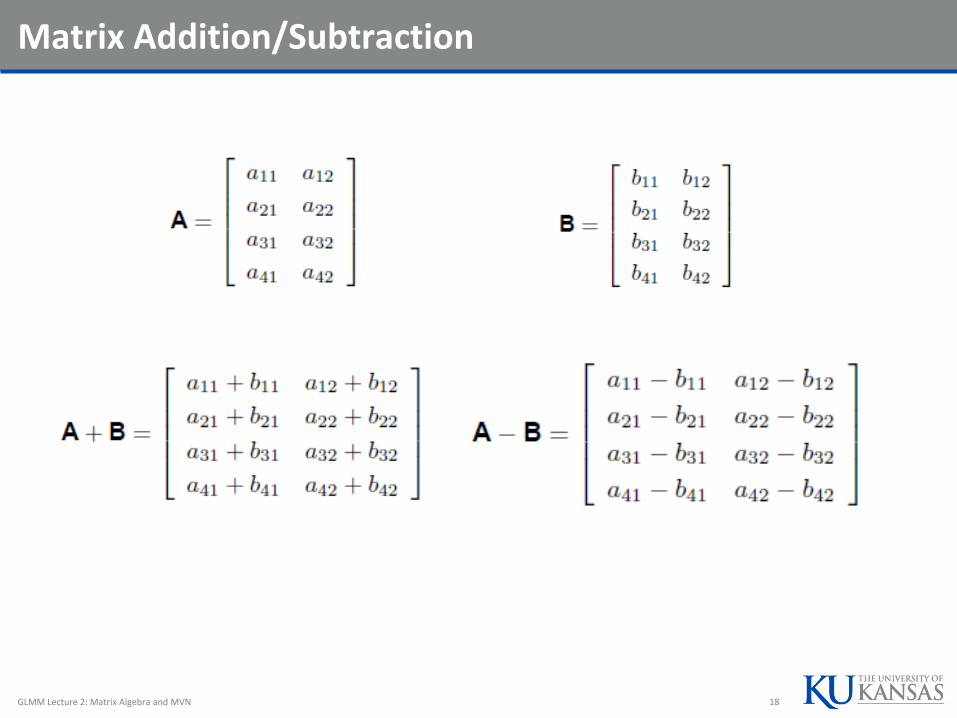
Matrix Addition/Subtraction
GLMM Lecture 2: Matrix Algebra and MVN 18
Matrix Multiplication
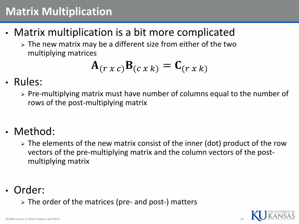
• Matrix multiplication is a bit more complicated The new matrix may be a different size from either of the two
multiplying matrices
𝐀(𝑟 𝑥 𝑐)𝐁(𝑐 𝑥 𝑘) = 𝐂(𝑟 𝑥 𝑘)• Rules:
Pre-multiplying matrix must have number of columns equal to the number of rows of the post-multiplying matrix
• Method: The elements of the new matrix consist of the inner (dot) product of the row
vectors of the pre-multiplying matrix and the column vectors of the post-multiplying matrix
• Order: The order of the matrices (pre- and post-) matters
GLMM Lecture 2: Matrix Algebra and MVN 19
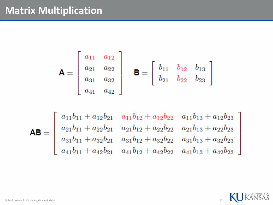
Matrix Multiplication
GLMM Lecture 2: Matrix Algebra and MVN 20
Multiplication in Statistics
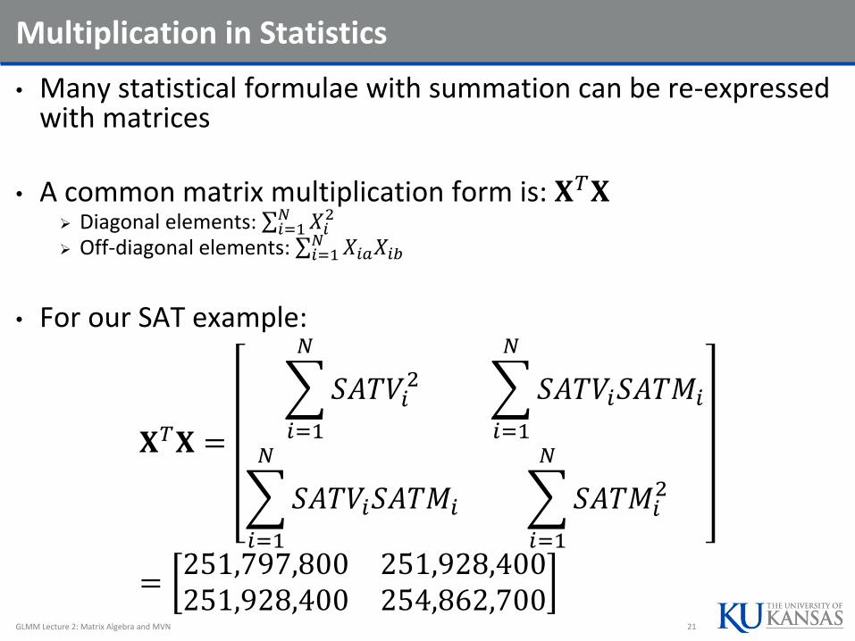
• Many statistical formulae with summation can be re-expressed with matrices
• A common matrix multiplication form is: 𝐗𝑇𝐗 Diagonal elements: 𝑖=1
𝑁 𝑋𝑖2
Off-diagonal elements: 𝑖=1𝑁 𝑋𝑖𝑎𝑋𝑖𝑏
• For our SAT example:
𝐗𝑇𝐗 =
𝑖=1
𝑁
𝑆𝐴𝑇𝑉𝑖2
𝑖=1
𝑁
𝑆𝐴𝑇𝑉𝑖𝑆𝐴𝑇𝑀𝑖
𝑖=1
𝑁
𝑆𝐴𝑇𝑉𝑖𝑆𝐴𝑇𝑀𝑖
𝑖=1
𝑁
𝑆𝐴𝑇𝑀𝑖2
=251,797,800 251,928,400251,928,400 254,862,700
GLMM Lecture 2: Matrix Algebra and MVN 21
Identity Matrix
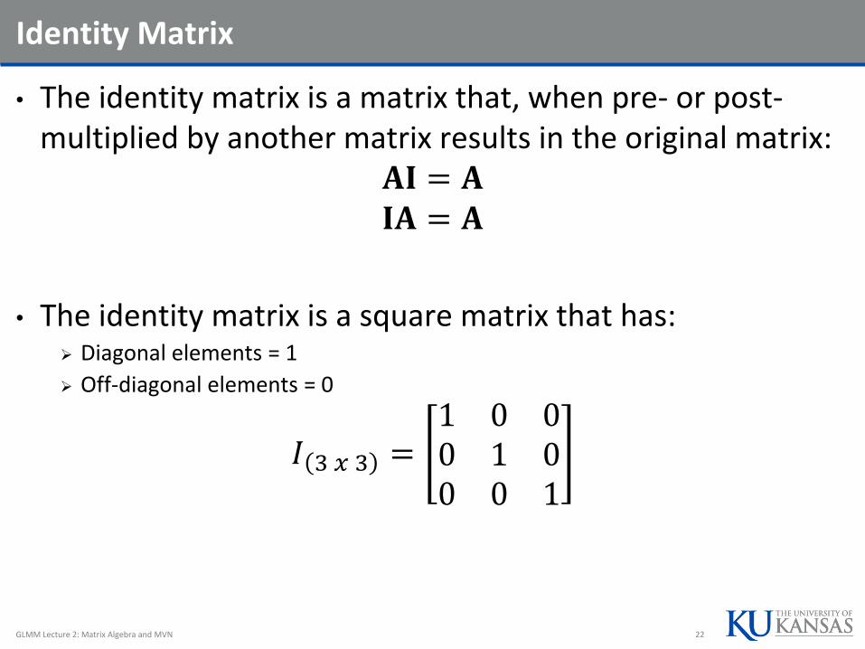
• The identity matrix is a matrix that, when pre- or post-multiplied by another matrix results in the original matrix:
𝐀𝐈 = 𝐀𝐈𝐀 = 𝐀
• The identity matrix is a square matrix that has: Diagonal elements = 1
Off-diagonal elements = 0
𝐼 3 𝑥 3 =1 0 00 1 00 0 1
GLMM Lecture 2: Matrix Algebra and MVN 22
Zero Vector
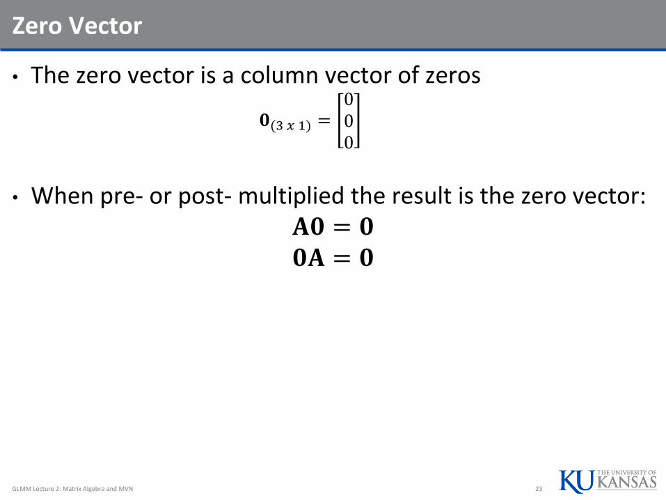
• The zero vector is a column vector of zeros
𝟎(3 𝑥 1) =000
• When pre- or post- multiplied the result is the zero vector:𝐀𝟎 = 𝟎𝟎𝐀 = 𝟎
GLMM Lecture 2: Matrix Algebra and MVN 23
Ones Vector
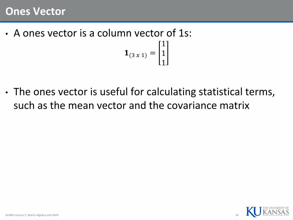
• A ones vector is a column vector of 1s:
𝟏(3 𝑥 1) =111
• The ones vector is useful for calculating statistical terms, such as the mean vector and the covariance matrix
GLMM Lecture 2: Matrix Algebra and MVN 24
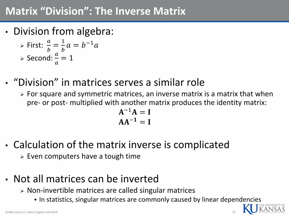
Matrix “Division”: The Inverse Matrix
• Division from algebra: First:
𝑎
𝑏=1
𝑏𝑎 = 𝑏−1𝑎
Second: 𝑎
𝑎= 1
• “Division” in matrices serves a similar role For square and symmetric matrices, an inverse matrix is a matrix that when
pre- or post- multiplied with another matrix produces the identity matrix:𝐀−1𝐀 = 𝐈𝐀𝐀−𝟏 = 𝐈
• Calculation of the matrix inverse is complicated Even computers have a tough time
• Not all matrices can be inverted Non-invertible matrices are called singular matrices
In statistics, singular matrices are commonly caused by linear dependencies
GLMM Lecture 2: Matrix Algebra and MVN 25
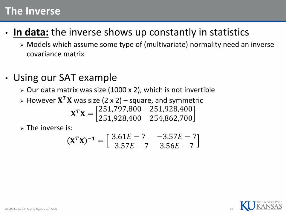
The Inverse
• In data: the inverse shows up constantly in statistics Models which assume some type of (multivariate) normality need an inverse
covariance matrix
• Using our SAT example Our data matrix was size (1000 x 2), which is not invertible
However 𝐗𝑇𝐗 was size (2 x 2) – square, and symmetric
𝐗𝑇𝐗 =251,797,800 251,928,400251,928,400 254,862,700
The inverse is:
𝐗𝑇𝐗 −1 =3.61𝐸 − 7 −3.57𝐸 − 7−3.57𝐸 − 7 3.56𝐸 − 7
GLMM Lecture 2: Matrix Algebra and MVN 26
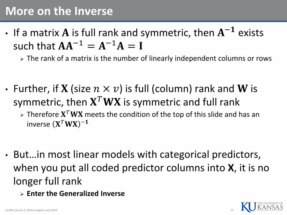
More on the Inverse
• If a matrix 𝐀 is full rank and symmetric, then 𝐀−𝟏 exists such that 𝐀𝐀−1 = 𝐀−1𝐀 = 𝐈
The rank of a matrix is the number of linearly independent columns or rows
• Further, if 𝐗 (size 𝑛 × 𝑣) is full (column) rank and 𝐖 is symmetric, then 𝐗𝑇𝐖𝐗 is symmetric and full rank
Therefore 𝐗𝑇𝐖𝐗meets the condition of the top of this slide and has an inverse 𝐗𝑇𝐖𝐗 −𝟏
• But…in most linear models with categorical predictors, when you put all coded predictor columns into X, it is no longer full rank
Enter the Generalized Inverse
GLMM Lecture 2: Matrix Algebra and MVN 27
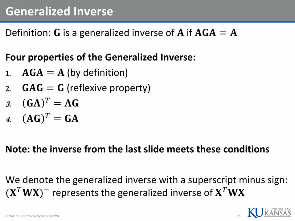
Generalized Inverse
Definition: 𝐆 is a generalized inverse of 𝐀 if 𝐀𝐆𝐀 = 𝐀
Four properties of the Generalized Inverse:
1. 𝐀𝐆𝐀 = 𝐀 (by definition)
2. 𝐆𝐀𝐆 = 𝐆 (reflexive property)
3. 𝐆𝐀 𝑇 = 𝐀𝐆
4. 𝐀𝐆 𝑇 = 𝐆𝐀
Note: the inverse from the last slide meets these conditions
We denote the generalized inverse with a superscript minus sign: (𝐗𝑇𝐖𝐗)− represents the generalized inverse of 𝐗𝑇𝐖𝐗
GLMM Lecture 2: Matrix Algebra and MVN 28
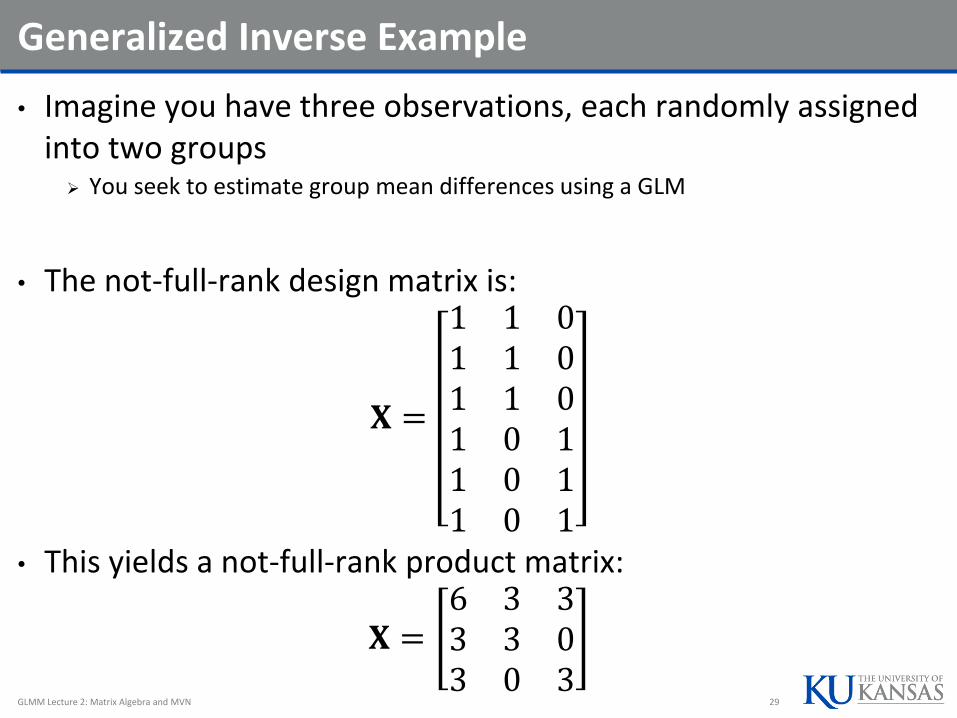
Generalized Inverse Example
• Imagine you have three observations, each randomly assigned into two groups
You seek to estimate group mean differences using a GLM
• The not-full-rank design matrix is:
𝐗 =
1 1 01 1 01 1 01 0 11 0 11 0 1
• This yields a not-full-rank product matrix:
𝐗 =6 3 33 3 03 0 3
GLMM Lecture 2: Matrix Algebra and MVN 29
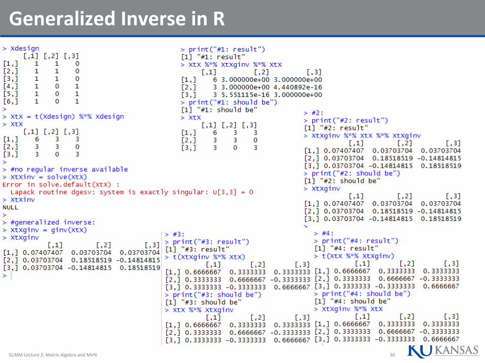
Generalized Inverse in R
GLMM Lecture 2: Matrix Algebra and MVN 30
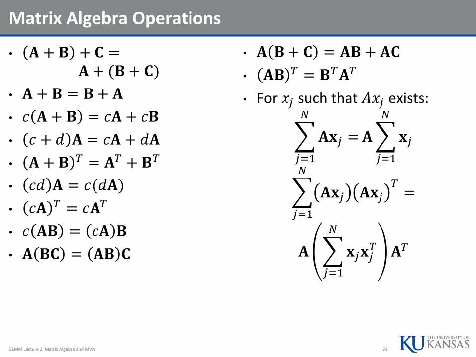
Matrix Algebra Operations
• 𝐀 + 𝐁 + 𝐂 =𝐀 + (𝐁 + 𝐂)
• 𝐀 + 𝐁 = 𝐁 + 𝐀
• 𝑐 𝐀 + 𝐁 = 𝑐𝐀 + 𝑐𝐁
• 𝑐 + 𝑑 𝐀 = 𝑐𝐀 + 𝑑𝐀
• 𝐀 + 𝐁 𝑇 = 𝐀𝑇 + 𝐁𝑇
• 𝑐𝑑 𝐀 = 𝑐(𝑑𝐀)
• 𝑐𝐀 𝑇 = 𝑐𝐀𝑇
• 𝑐 𝐀𝐁 = 𝑐𝐀 𝐁
• 𝐀 𝐁𝐂 = 𝐀𝐁 𝐂
• 𝐀 𝐁 + 𝐂 = 𝐀𝐁 + 𝐀𝐂
• 𝐀𝐁 𝑇 = 𝐁𝑇𝐀𝑇
• For 𝑥𝑗 such that 𝐴𝑥𝑗 exists:
𝑗=1
𝑁
𝐀𝐱𝑗 =𝐀
𝑗=1
𝑁
𝐱𝑗
𝑗=1
𝑁
𝐀𝐱𝑗 𝐀𝐱𝑗𝑇=
𝐀
𝑗=1
𝑁
𝐱𝑗𝐱𝑗𝑇 𝐀𝑇
GLMM Lecture 2: Matrix Algebra and MVN 31
BIVARIATE NORMAL DISTRIBUTION
A Multivariate Distribution with Two Variables
GLMM Lecture 2: Matrix Algebra and MVN 32
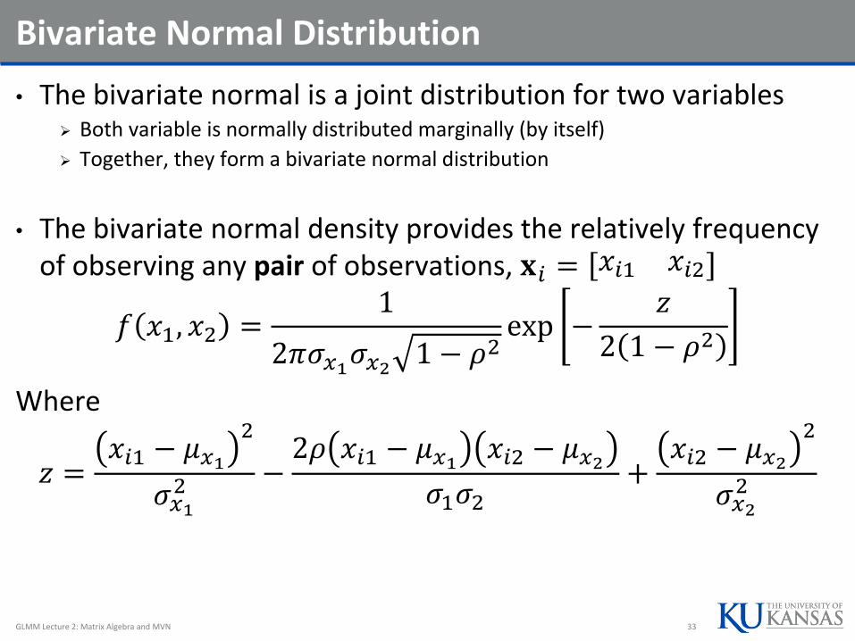
Bivariate Normal Distribution
• The bivariate normal is a joint distribution for two variables Both variable is normally distributed marginally (by itself)
Together, they form a bivariate normal distribution
• The bivariate normal density provides the relatively frequency of observing any pair of observations, 𝐱𝑖 = 𝑥𝑖1 𝑥𝑖2
𝑓 𝑥1, 𝑥2 =1
2𝜋𝜎𝑥1𝜎𝑥2 1 − 𝜌2exp −
𝑧
2 1 − 𝜌2
Where
𝑧 =𝑥𝑖1 − 𝜇𝑥1
2
𝜎𝑥12 −
2𝜌 𝑥𝑖1 − 𝜇𝑥1 𝑥𝑖2 − 𝜇𝑥2𝜎1𝜎2
+𝑥𝑖2 − 𝜇𝑥2
2
𝜎𝑥22
GLMM Lecture 2: Matrix Algebra and MVN 33

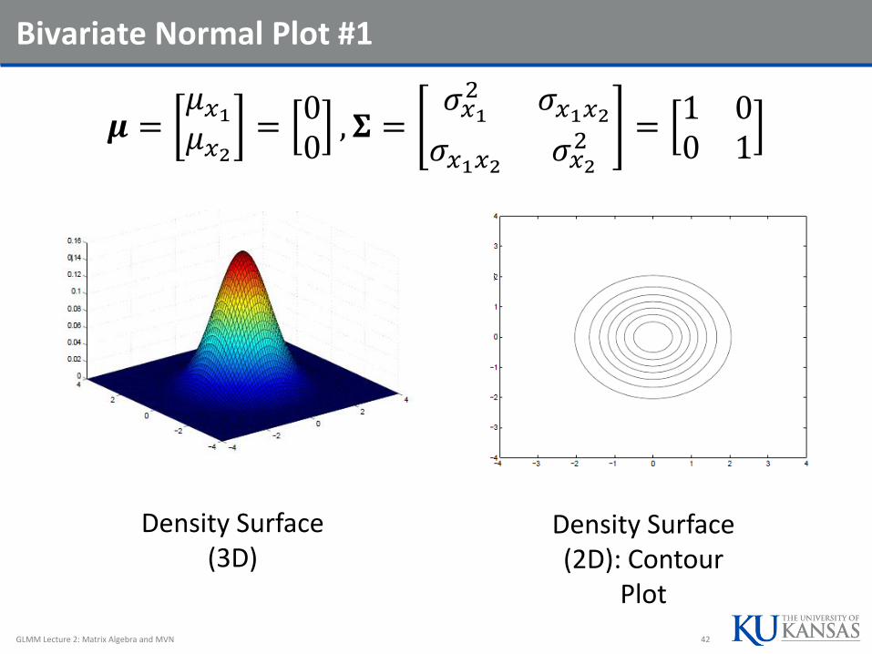
Bivariate Normal Plot #1
𝝁 =𝜇𝑥1𝜇𝑥2=00, 𝚺 =
𝜎𝑥12 𝜎𝑥1𝑥2𝜎𝑥1𝑥2 𝜎𝑥2
2 =1 00 1
Density Surface (3D)
Density Surface (2D): Contour
Plot
GLMM Lecture 2: Matrix Algebra and MVN 34
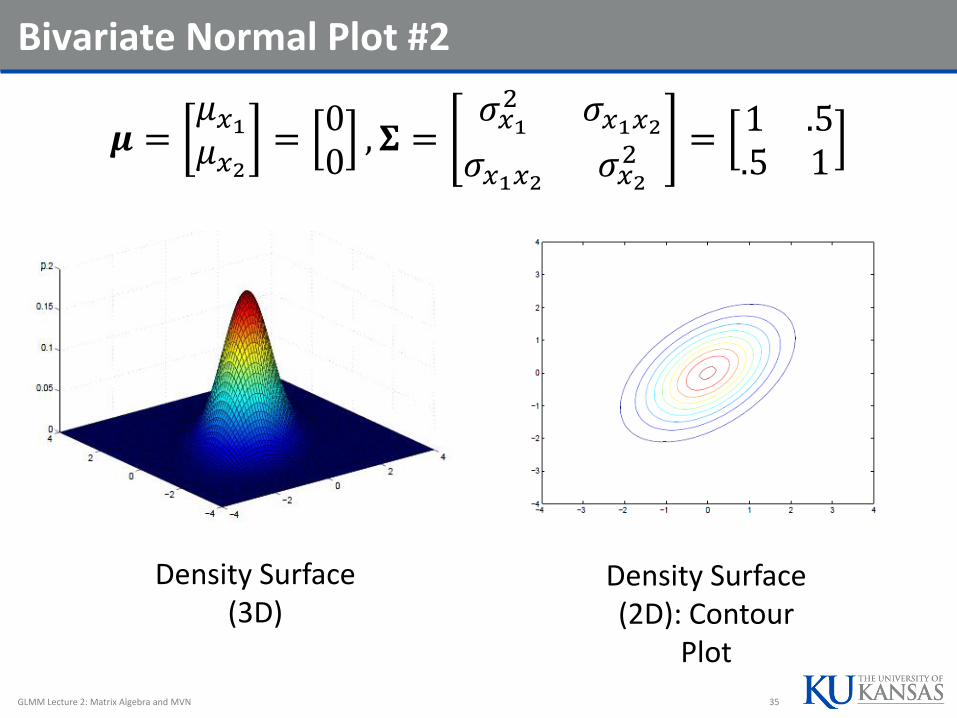
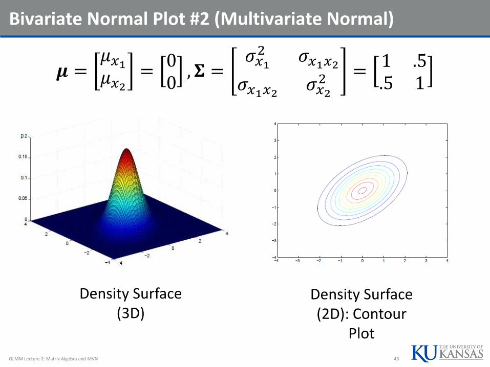
Bivariate Normal Plot #2
𝝁 =𝜇𝑥1𝜇𝑥2=00, 𝚺 =
𝜎𝑥12 𝜎𝑥1𝑥2𝜎𝑥1𝑥2 𝜎𝑥2
2 =1 .5.5 1
Density Surface (3D)
Density Surface (2D): Contour
Plot
GLMM Lecture 2: Matrix Algebra and MVN 35
MULTIVARIATE NORMAL DISTRIBUTIONS (VARIABLES ≥ 2)
GLMM Lecture 2: Matrix Algebra and MVN 36
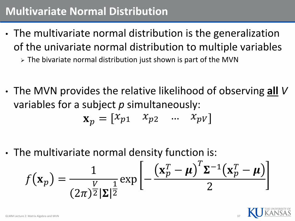
Multivariate Normal Distribution
• The multivariate normal distribution is the generalization of the univariate normal distribution to multiple variables
The bivariate normal distribution just shown is part of the MVN
• The MVN provides the relative likelihood of observing all V variables for a subject p simultaneously:
𝐱𝑝 = 𝑥𝑝1 𝑥𝑝2 … 𝑥𝑝𝑉
• The multivariate normal density function is:
𝑓 𝐱𝑝 =1
2𝜋𝑉2 𝚺12
exp −𝐱𝑝𝑇 − 𝝁
𝑇𝚺−1 𝐱𝑝
𝑇 − 𝝁
2
GLMM Lecture 2: Matrix Algebra and MVN 37
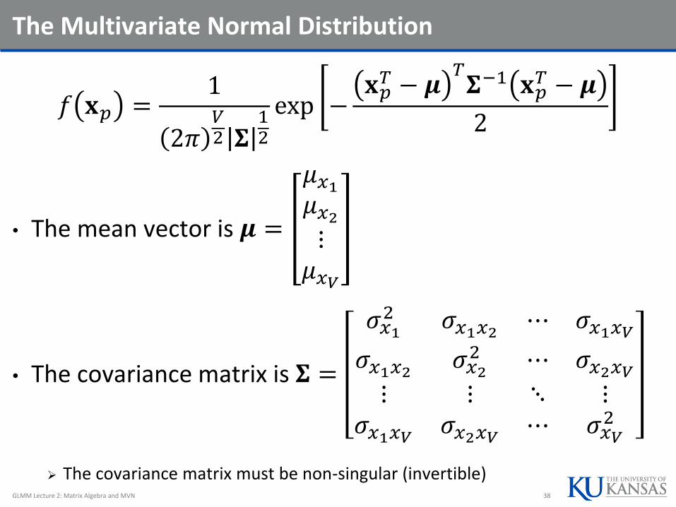
The Multivariate Normal Distribution
𝑓 𝐱𝑝 =1
2𝜋𝑉2 𝚺12
exp −𝐱𝑝𝑇 − 𝝁
𝑇𝚺−1 𝐱𝑝
𝑇 − 𝝁
2
• The mean vector is 𝝁 =
𝜇𝑥1𝜇𝑥2⋮𝜇𝑥𝑉
• The covariance matrix is 𝚺 =
𝜎𝑥12 𝜎𝑥1𝑥2 ⋯ 𝜎𝑥1𝑥𝑉𝜎𝑥1𝑥2 𝜎𝑥2
2 ⋯ 𝜎𝑥2𝑥𝑉⋮ ⋮ ⋱ ⋮𝜎𝑥1𝑥𝑉 𝜎𝑥2𝑥𝑉 ⋯ 𝜎𝑥𝑉
2
The covariance matrix must be non-singular (invertible)GLMM Lecture 2: Matrix Algebra and MVN 38
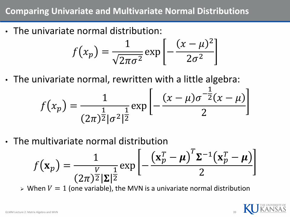
Comparing Univariate and Multivariate Normal Distributions
• The univariate normal distribution:
𝑓 𝑥𝑝 =1
2𝜋𝜎2exp −
𝑥 − 𝜇 2
2𝜎2
• The univariate normal, rewritten with a little algebra:
𝑓 𝑥𝑝 =1
2𝜋12|𝜎2|
12
exp −𝑥 − 𝜇 𝜎−
12 𝑥 − 𝜇
2
• The multivariate normal distribution
𝑓 𝐱𝑝 =1
2𝜋𝑉2 𝚺12
exp −𝐱𝑝𝑇 − 𝝁
𝑇𝚺−1 𝐱𝑝
𝑇 − 𝝁
2
When 𝑉 = 1 (one variable), the MVN is a univariate normal distribution
GLMM Lecture 2: Matrix Algebra and MVN 39
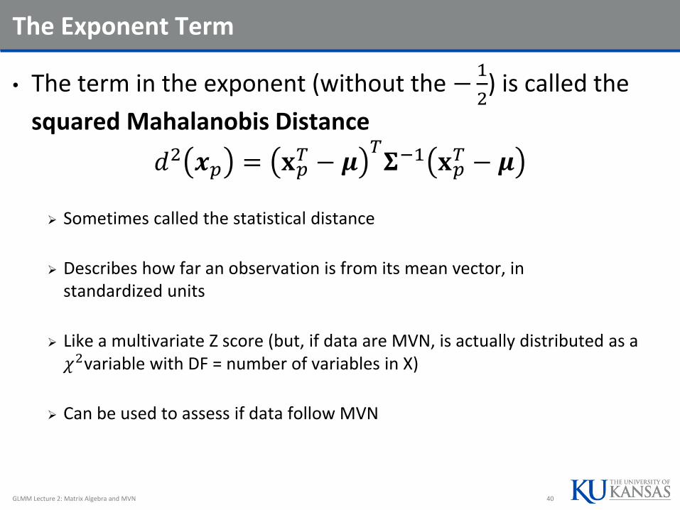
The Exponent Term
• The term in the exponent (without the −1
2) is called the
squared Mahalanobis Distance
𝑑2 𝒙𝑝 = 𝐱𝑝𝑇 − 𝝁
𝑇𝚺−1 𝐱𝑝
𝑇 − 𝝁
Sometimes called the statistical distance
Describes how far an observation is from its mean vector, in standardized units
Like a multivariate Z score (but, if data are MVN, is actually distributed as a 𝜒2variable with DF = number of variables in X)
Can be used to assess if data follow MVN
GLMM Lecture 2: Matrix Algebra and MVN 40
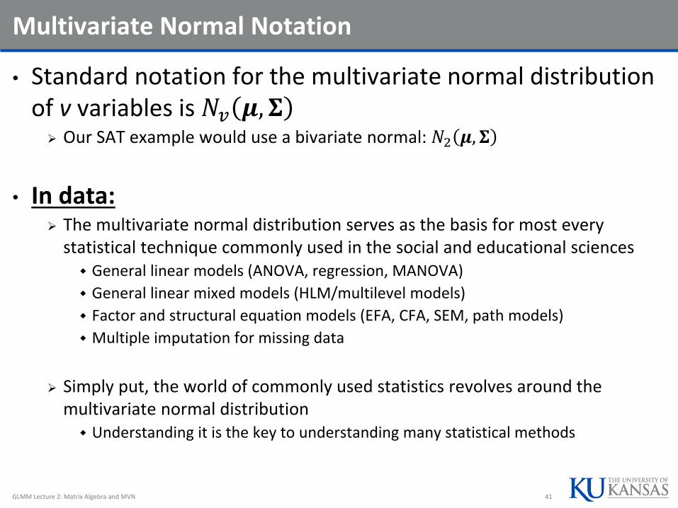
Multivariate Normal Notation
• Standard notation for the multivariate normal distribution of v variables is 𝑁𝑣 𝝁, 𝚺
Our SAT example would use a bivariate normal: 𝑁2 𝝁, 𝚺
• In data: The multivariate normal distribution serves as the basis for most every
statistical technique commonly used in the social and educational sciences General linear models (ANOVA, regression, MANOVA)
General linear mixed models (HLM/multilevel models)
Factor and structural equation models (EFA, CFA, SEM, path models)
Multiple imputation for missing data
Simply put, the world of commonly used statistics revolves around the multivariate normal distribution Understanding it is the key to understanding many statistical methods
GLMM Lecture 2: Matrix Algebra and MVN 41
Bivariate Normal Plot #1
𝝁 =𝜇𝑥1𝜇𝑥2=00, 𝚺 =
𝜎𝑥12 𝜎𝑥1𝑥2𝜎𝑥1𝑥2 𝜎𝑥2
2 =1 00 1
GLMM Lecture 2: Matrix Algebra and MVN 42
Density Surface (3D)
Density Surface (2D): Contour
Plot
Bivariate Normal Plot #2 (Multivariate Normal)
𝝁 =𝜇𝑥1𝜇𝑥2=00, 𝚺 =
𝜎𝑥12 𝜎𝑥1𝑥2𝜎𝑥1𝑥2 𝜎𝑥2
2 =1 .5.5 1
GLMM Lecture 2: Matrix Algebra and MVN 43
Density Surface (3D)
Density Surface (2D): Contour
Plot
Multivariate Normal Properties
• The multivariate normal distribution has some useful properties that show up in statistical methods
• If 𝐗 is distributed multivariate normally:
1. Linear combinations of 𝐗 are normally distributed
2. All subsets of 𝐗 are multivariate normally distributed
3. A zero covariance between a pair of variables of 𝐗implies that the variables are independent
4. Conditional distributions of 𝐗 are multivariate normal
GLMM Lecture 2: Matrix Algebra and MVN 44
Multivariate Normal Distribution
• To demonstrate how the MVN works, we will now investigate how the PDF provides the likelihood (height) for a given observation:
Here we will use the SAT data and assume the sample mean vector and covariance matrix are known to be the true:
𝝁 =499.32498.27
; 𝐒 =2,477.34 3,123.223,132.22 6,589.71
• We will compute the likelihood value for several observations (SEE EXAMPLE R SYNTAX FOR HOW THIS WORKS):
𝒙631,⋅ = 590 730 ; 𝑓 𝒙 = 0.0000001393048
𝒙717,⋅ = 340 300 ; 𝑓 𝒙 = 0.0000005901861 𝒙 = 𝒙 = 499.32 498.27 ; 𝑓 𝒙 = 0.000009924598
• Note: this is the height for these observations, not the joint likelihood across all the data
Next time we will use PROC MIXED to find the parameters in 𝝁 and 𝚺 using maximum likelihood
PRE 905: Lecture 7 -- Matrix Algebra and the MVN Distribution 45
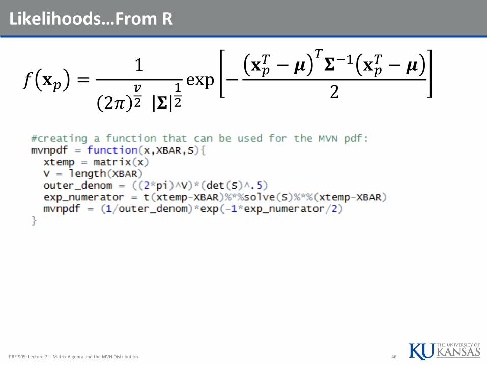
Likelihoods…From R
PRE 905: Lecture 7 -- Matrix Algebra and the MVN Distribution 46
𝑓 𝐱𝑝 =1
2𝜋𝑣2 𝚺
12
exp −𝐱𝑝𝑇 − 𝝁
𝑇𝚺−1 𝐱𝑝
𝑇 − 𝝁
2

ADDITIONAL LECTURE WITHOUT SLIDES
GLMM Lecture 2: Matrix Algebra and MVN 47