2. Matrix Algebra and Random Vectors

2.1 Introduction

Multivariate data can be conveniently display as array of numbers. In general,a rectangular array of numbers with, for instance, n rows and p columns iscalled a matrix of dimension n× p The study of multivariate methods is greatlyfacilitated by the use of matrix algebra.

1

2.2 Some Basic of Matrix and Vector Algebra

Vectors

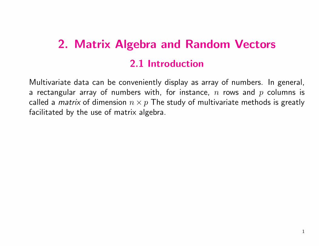
• Definition: An array x of n real number x1, x2, . . . , xn is called a vector, andit is written as

x =

x1

x2...

xn

or x′ = [x1, x2, . . . , xn]

where the prime denotes the operation of transposing a column to a row.

2

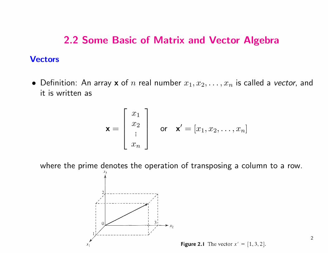
• Multiplying vectors by a constant c:

cx = x =

cx1

cx2...

cxn

• Addition of x and y is defined as

x + y =

x1

x2...

xn

+

y1

y2...

yn

=

x1 + y1

x2 + y2...

xn + yn

3

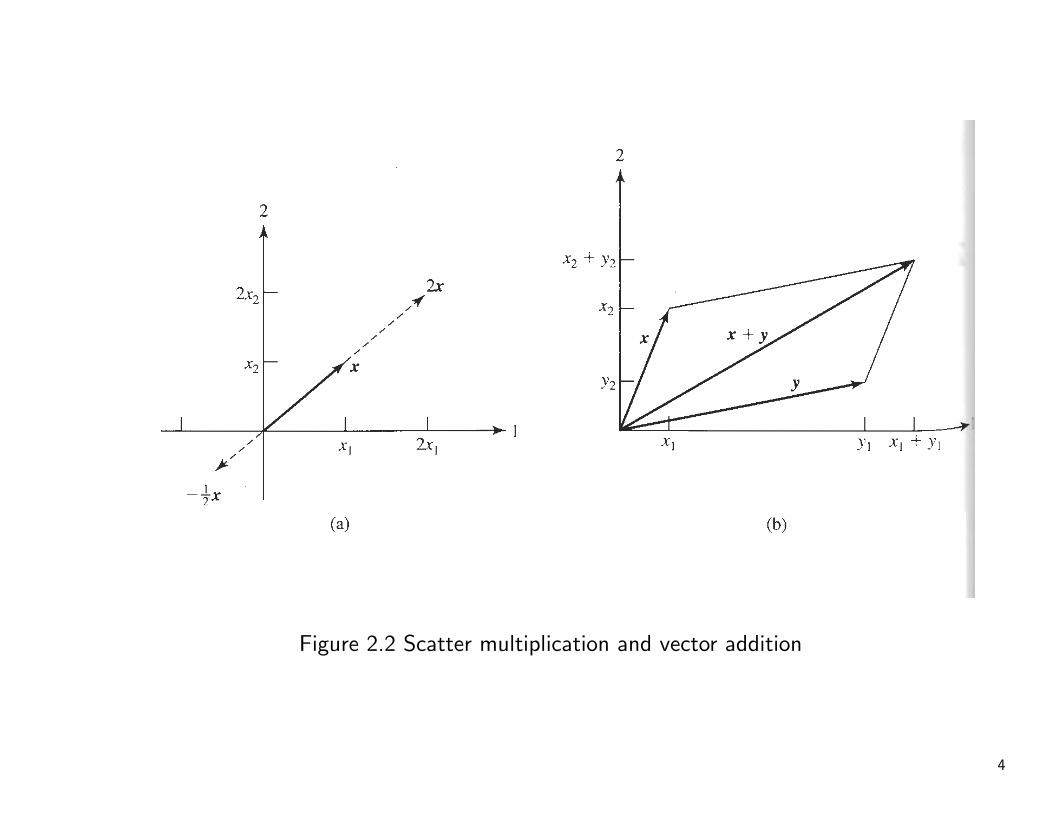
Figure 2.2 Scatter multiplication and vector addition

4

• Length of vectors, unit vector

When n = 2, x = [x1, x2]′, the length of x, written Lx is defined to be

Lx =√

x21 + x2

2

Geometrically, the length of a vector in two dimension can be viewed as thehypotenuse of a right triangle. The length of a vector x = [x1, x2, . . . , xn]′

and cx = [cx1, cx2, . . . , cxn]′

Lx =√

x21 + x2

2 + · · ·+ x2n

Lcx =√

c2x21 + c2x2

2 + · · ·+ c2x2n = |c|

√x2

1 + x22 + · · ·+ x2

n = |c|Lx

Choosing c = L−1x , we obtain the unit vector L−1

x x, which has length 1 andlies in the direction of x.

5

6

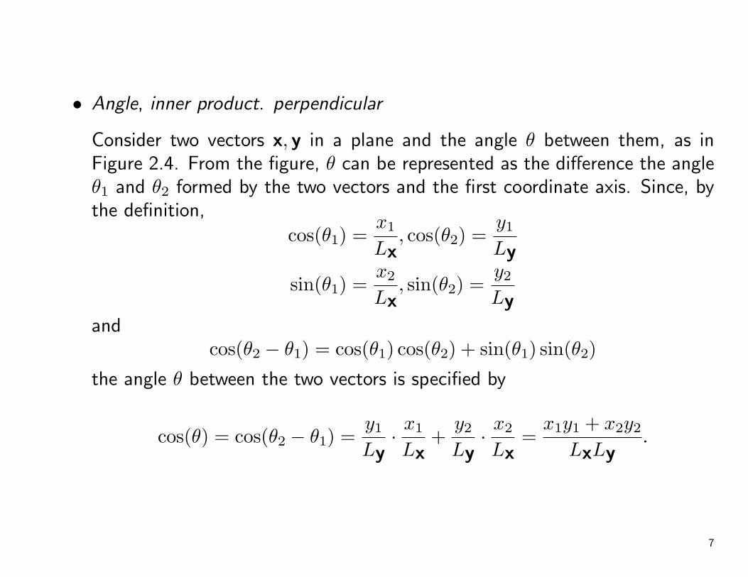
• Angle, inner product. perpendicular

Consider two vectors x, y in a plane and the angle θ between them, as inFigure 2.4. From the figure, θ can be represented as the difference the angleθ1 and θ2 formed by the two vectors and the first coordinate axis. Since, bythe definition,

cos(θ1) =x1

Lx, cos(θ2) =

y1

Ly

sin(θ1) =x2

Lx, sin(θ2) =

y2

Lyand

cos(θ2 − θ1) = cos(θ1) cos(θ2) + sin(θ1) sin(θ2)

the angle θ between the two vectors is specified by

cos(θ) = cos(θ2 − θ1) =y1

Ly· x1

Lx+

y2

Ly· x2

Lx=

x1y1 + x2y2

LxLy.

7

• Definition of inner product of the two vectors x and y

x′y = x1y1 + x2y2.

With the definition of the inner product and cos(θ),

Lx =√

x′x, cos(θ) =x′y

LxLy=

x′y√x′x√

y′y.

Example 2.1.(Calculating lengths of vectors and the angle between them)Given the vectors x′ = [132] and y′ = [−21 − 1], find 3x and x + y. Next,determine the length of x, the length of y, and the angle between x and y.Also, check that the length of 3x is three times the length of x

8

• A pair of vectors x and y of the same dimension is said to be linearlydependent if there exist constants c1 and c2, both not zero, such thatc1x + c2y = 0. A set of vectors x1, x2, . . . , xk is said to be linearly dependentif there exist constants c1, c2, . . . , ck, not all zero, such that

c1x1 + c2x2 + . . . + ckxk = 0.

Linear dependence implies that at least one vector in the set can be writtenas linear combination of the other vectors. Vector of the same dimensionthat are not linearly dependent are said to be linearly independent.

9

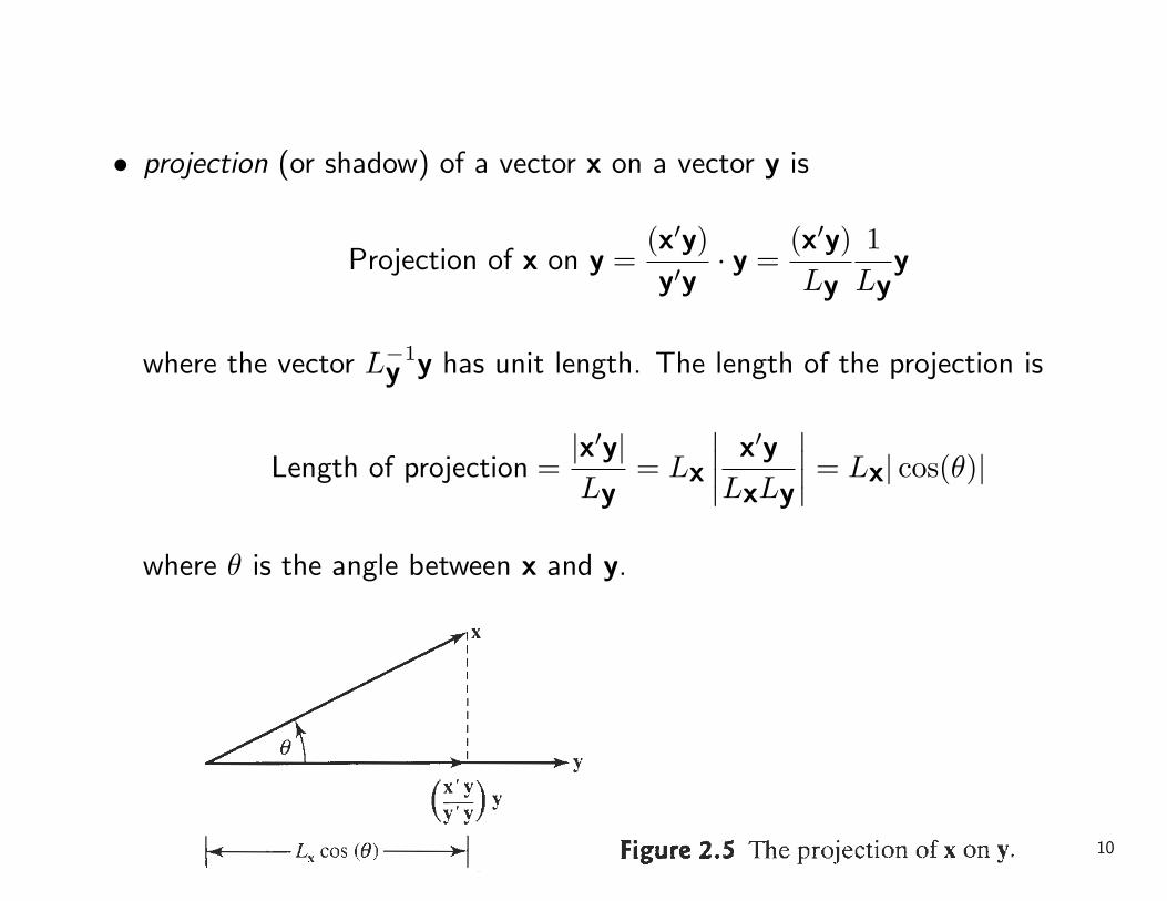
• projection (or shadow) of a vector x on a vector y is

Projection of x on y =(x′y)y′y

· y =(x′y)Ly

1Ly

y

where the vector L−1y y has unit length. The length of the projection is

Length of projection =|x′y|Ly

= Lx

∣∣∣∣ x′y

LxLy

∣∣∣∣ = Lx| cos(θ)|

where θ is the angle between x and y.

10

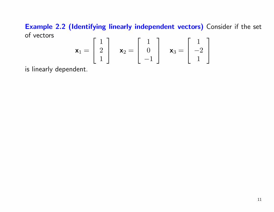
Example 2.2 (Identifying linearly independent vectors) Consider if the setof vectors

x1 =

121

x2 =

10−1

x3 =

1−21

is linearly dependent.

11

Matrices

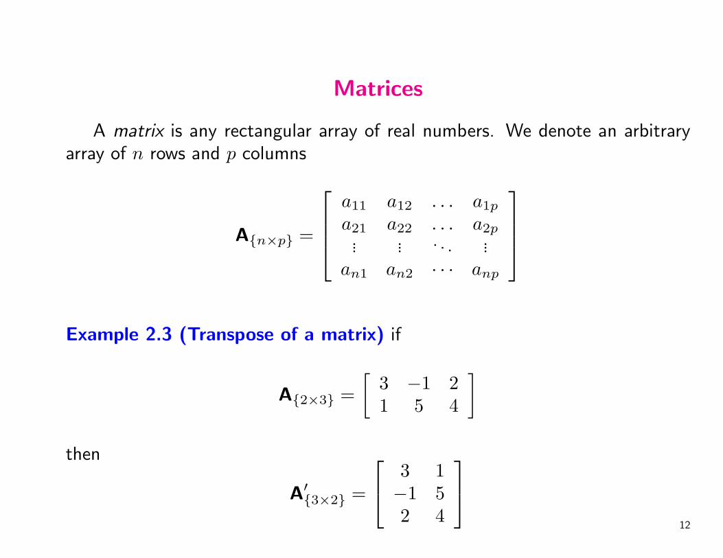
A matrix is any rectangular array of real numbers. We denote an arbitraryarray of n rows and p columns

A{n×p} =

a11 a12 . . . a1p

a21 a22 . . . a2p... ... . . . ...

an1 an2 · · · anp

Example 2.3 (Transpose of a matrix) if

A{2×3} =[

3 −1 21 5 4

]then

A′{3×2} =

3 1−1 52 4

12

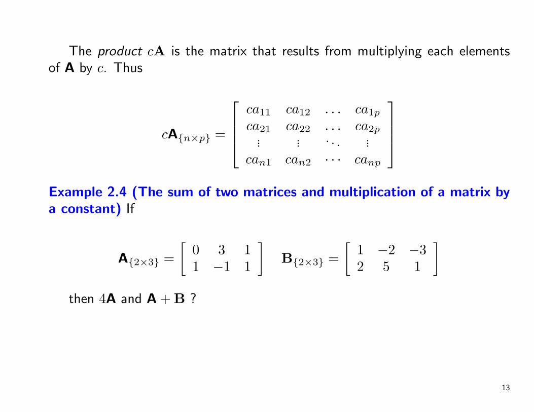
The product cA is the matrix that results from multiplying each elementsof A by c. Thus

cA{n×p} =

ca11 ca12 . . . ca1p

ca21 ca22 . . . ca2p... ... . . . ...

can1 can2 · · · canp

Example 2.4 (The sum of two matrices and multiplication of a matrix bya constant) If

A{2×3} =[

0 3 11 −1 1

]B{2×3} =

[1 −2 −32 5 1

]then 4A and A + B ?

13

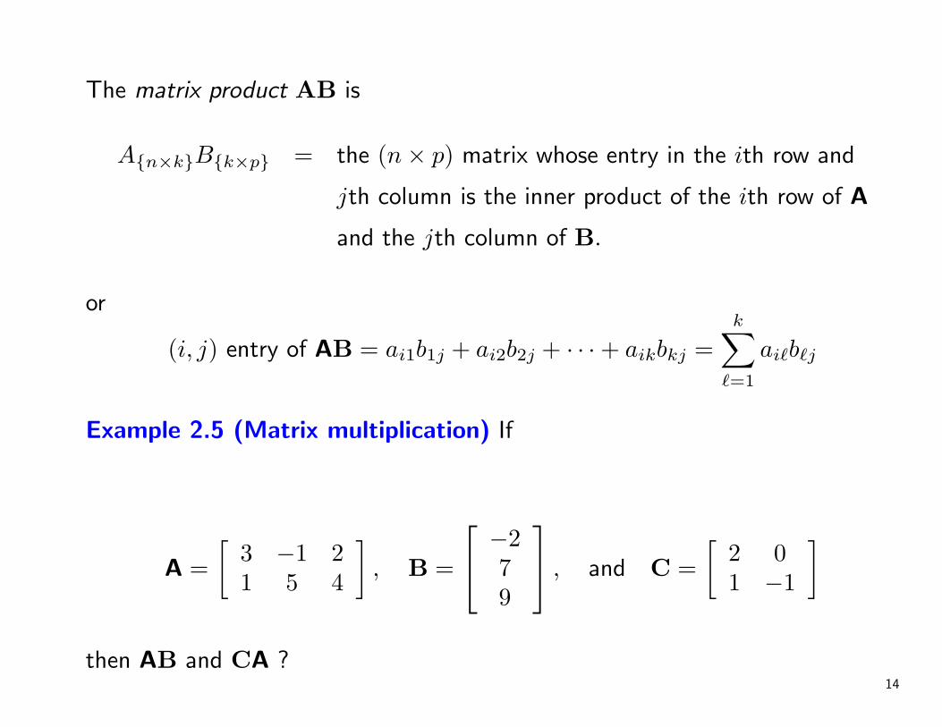
The matrix product AB is

A{n×k}B{k×p} = the (n× p) matrix whose entry in the ith row and

jth column is the inner product of the ith row of A

and the jth column of B.

or

(i, j) entry of AB = ai1b1j + ai2b2j + · · ·+ aikbkj =k∑

`=1

ai`b`j

Example 2.5 (Matrix multiplication) If

A =[

3 −1 21 5 4

], B =

−279

, and C =[

2 01 −1

]

then AB and CA ?14

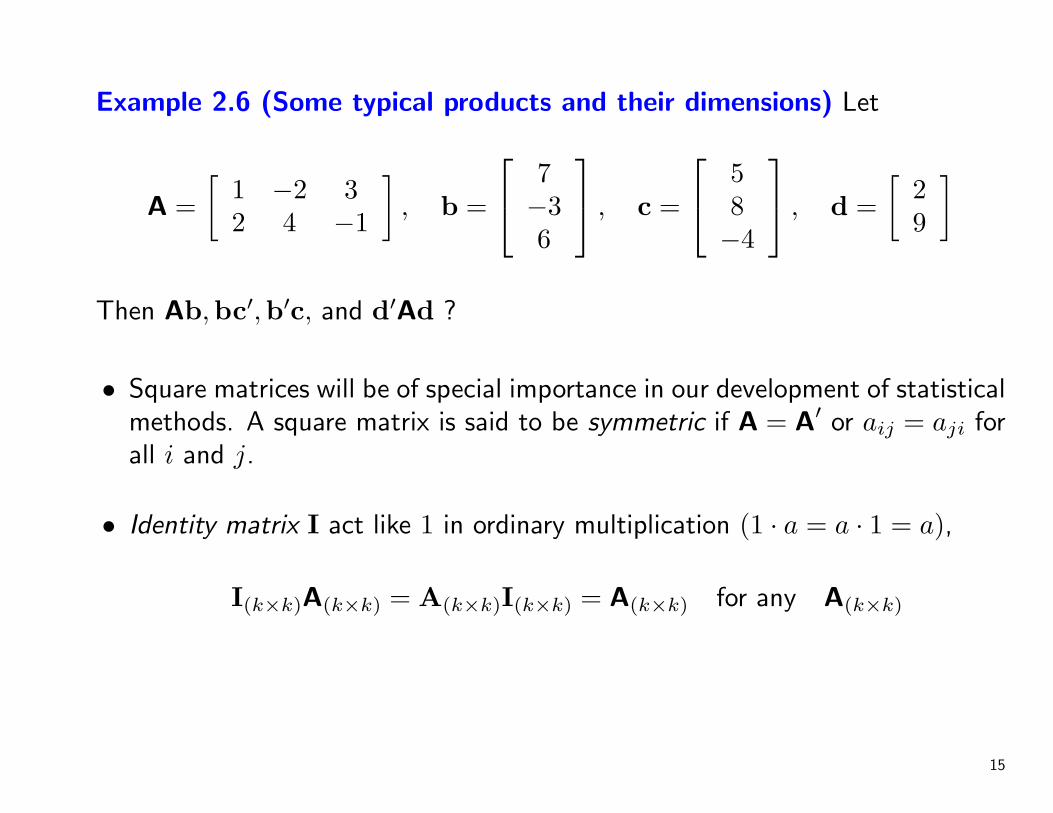
Example 2.6 (Some typical products and their dimensions) Let

A =[

1 −2 32 4 −1

], b =

7−36

, c =

58−4

, d =[

29

]

Then Ab,bc′,b′c, and d′Ad ?

• Square matrices will be of special importance in our development of statisticalmethods. A square matrix is said to be symmetric if A = A′ or aij = aji forall i and j.

• Identity matrix I act like 1 in ordinary multiplication (1 · a = a · 1 = a),

I(k×k)A(k×k) = A(k×k)I(k×k) = A(k×k) for any A(k×k)

15

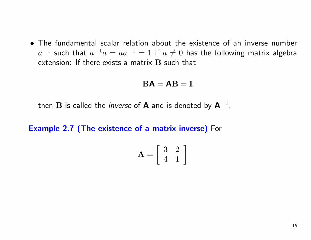
• The fundamental scalar relation about the existence of an inverse numbera−1 such that a−1a = aa−1 = 1 if a 6= 0 has the following matrix algebraextension: If there exists a matrix B such that

BA = AB = I

then B is called the inverse of A and is denoted by A−1.

Example 2.7 (The existence of a matrix inverse) For

A =[

3 24 1

]

16

• Diagonal matrices

• Orthogonal matrices

QQ′ = Q′Q = I or Q′ = Q−1.

• Eigenvalue λ with corresponding eigenvector x 6= 0 if

Ax = λx

Ordinarily, x is normalized so that it has length unity; that is x′x = 1.

17

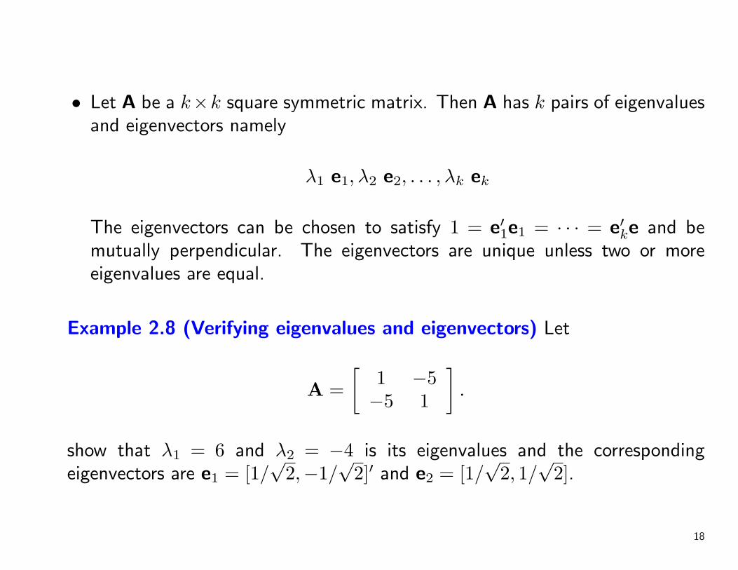
• Let A be a k×k square symmetric matrix. Then A has k pairs of eigenvaluesand eigenvectors namely

λ1 e1, λ2 e2, . . . , λk ek

The eigenvectors can be chosen to satisfy 1 = e′1e1 = · · · = e′ke and bemutually perpendicular. The eigenvectors are unique unless two or moreeigenvalues are equal.

Example 2.8 (Verifying eigenvalues and eigenvectors) Let

A =[

1 −5−5 1

].

show that λ1 = 6 and λ2 = −4 is its eigenvalues and the correspondingeigenvectors are e1 = [1/

√2,−1/

√2]′ and e2 = [1/

√2, 1/

√2].

18

2.3 Positive Definite Matrices

The study of variation and interrelationships in multivariate data is oftenbased upon distances and the assumption that the data are multivariate normallydistributed. Squared distance and the multivariate normal density can beexpressed in terms of matrix products called quadratic forms. Consequently,it should not be surprising that quadratic forms play central role in multivariateanalysis. Quadratic forms that are always nonnegative and the associatedpositive definite matrices.

• spectral decomposition for symmetric matrices

A(k×k) = λ1e1e′1 + λ1e2e

′2 + · · ·+ λ1eke

′k

where λ1, λ2, . . . , λk are the eigenvalues and e1, e2, . . . , ek are the associatednormalized k × 1 eigenvectors. e′iei = 1 for i = 1, 2, . . . , k and e′iej = 0 fori 6= j.

19

• Because x′Ax has only square terms x2i and product terms xixk, it is called

a quadratic form. When a k × k symmetric matrix A is such that

0 ≤ x′Ax

for all x′ = [x1, x2, . . . , xk], both the matrix A and the quadratic form aresaid to be nonnegative definite. If the equality holds in the equationabove only for the vector x′ = [0, 0, . . . , 0], then A or the quadratic form issaid to be positive definite. In other words, A is positive definite if

0 < x′Ax

for all vectors x 6= 0.

• Using the spectral decomposition, we can easily show that a k × k matrix Ais a positive definite matrix if and only if every eigenvalue of A is positive. Ais a nonnegative definite matrix if and only if all of its eigenvalues are greaterthan or equal to zero.

20

Example 2.9 ( The spectral decomposition of a matrix) Consider thesymmetric matrix

A =

13 −4 2−4 13 −22 −2 10

,

find its spectral decomposition.

Example 2.10 ( A positive definite matrix quadratic form) Show that thematrix for the following quadratic form is positive definite:

3x21 + 2x2

2 − 2√

2x1x2.

• the “distance ” of the point [x1, x2, . . . , xp]′ to origin

(distance)2 = a11x21 + a22x

22 + . . . + a2

pp

+2(a12x1x2 + a13x1x3 + . . . + ap−1,pxp−1xp)

• the square of the distance x to an arbitrary fixed point µ = [µ1, µ2, . . . , µp].21

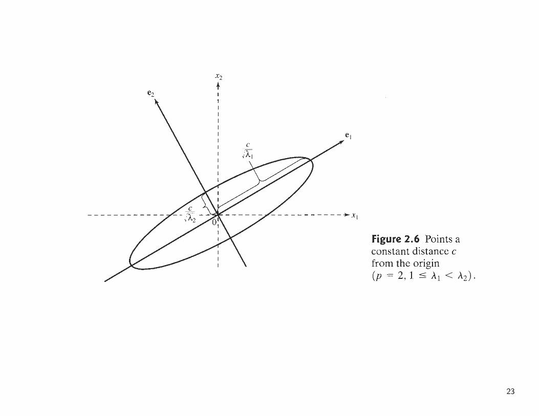
• A geometric interpretation based on the eigenvalues and eigenvectors of thematrix A.

For example, suppose p = 2, Then the points x′ = [x1, x2] of constantdistance c from the origin satisfy

x′Ax = a11x21 + a2

22 + 2a12x1x2 = c2

By the spectral decomposition,

A = λ1e1e′1 + λ2e2e

′2

sox′Ax = λ1(x′e1)2 + λ2(x′e2)2

22

23

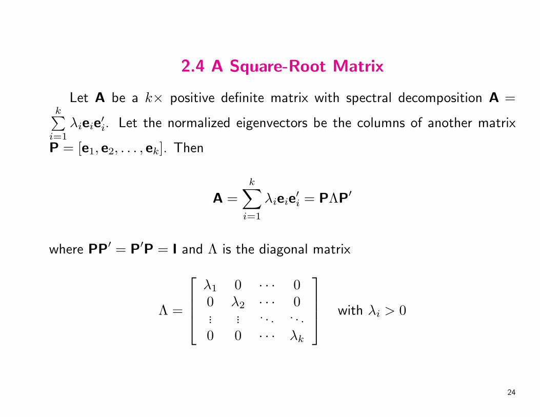
2.4 A Square-Root Matrix

Let A be a k× positive definite matrix with spectral decomposition A =k∑

i=1

λieie′i. Let the normalized eigenvectors be the columns of another matrix

P = [e1, e2, . . . , ek]. Then

A =k∑

i=1

λieie′i = PΛP′

where PP′ = P′P = I and Λ is the diagonal matrix

Λ =

λ1 0 · · · 00 λ2 · · · 0... ... . . . . . .0 0 · · · λk

with λi > 0

24

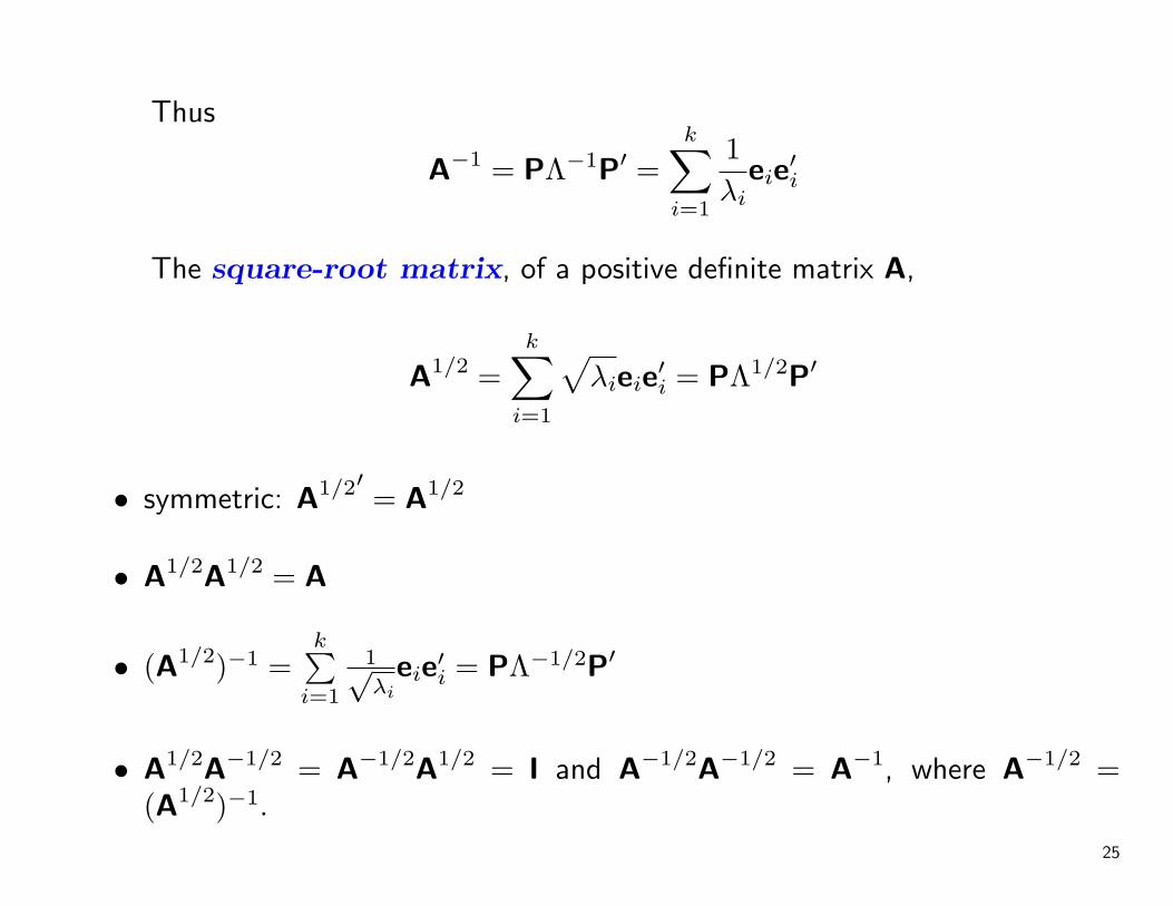
Thus

A−1 = PΛ−1P′ =k∑

i=1

1λi

eie′i

The square-root matrix, of a positive definite matrix A,

A1/2 =k∑

i=1

√λieie

′i = PΛ1/2P′

• symmetric: A1/2′ = A1/2

• A1/2A1/2 = A

• (A1/2)−1 =k∑

i=1

1√λi

eie′i = PΛ−1/2P′

• A1/2A−1/2 = A−1/2A1/2 = I and A−1/2A−1/2 = A−1, where A−1/2 =(A1/2)−1.

25

Random Vectors and Matrices

A random vector is a vector whose elements are random variables.Similarly a random matrix is a matrix whose elements are random variables.

• The expected value of a random matrix

E(X) =

E(X11) E(X12) · · · E(X1p)E(X21) E(X22) · · · E(X2p)

... ... . . . ...E(Xn1) E(Xn2) · · · E(Xnp)

• E(X + Y ) = E(X) + E(Y )

• E(AXB) = AE(X)B

26

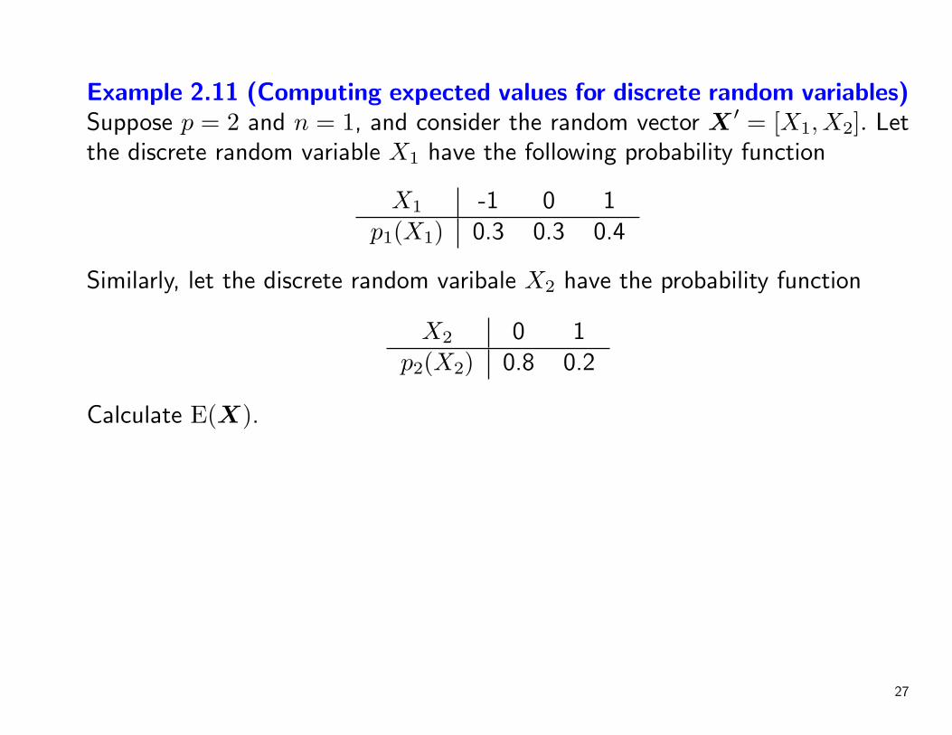
Example 2.11 (Computing expected values for discrete random variables)Suppose p = 2 and n = 1, and consider the random vector X ′ = [X1, X2]. Letthe discrete random variable X1 have the following probability function

X1 -1 0 1p1(X1) 0.3 0.3 0.4

Similarly, let the discrete random varibale X2 have the probability function

X2 0 1p2(X2) 0.8 0.2

Calculate E(X).

27

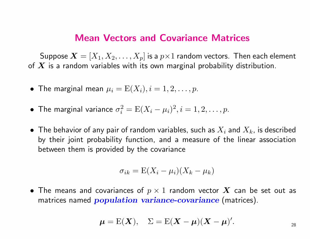
Mean Vectors and Covariance Matrices

Suppose X = [X1, X2, . . . , Xp] is a p×1 random vectors. Then each elementof X is a random variables with its own marginal probability distribution.

• The marginal mean µi = E(Xi), i = 1, 2, . . . , p.

• The marginal variance σ2i = E(Xi − µi)2, i = 1, 2, . . . , p.

• The behavior of any pair of random variables, such as Xi and Xk, is describedby their joint probability function, and a measure of the linear associationbetween them is provided by the covariance

σik = E(Xi − µi)(Xk − µk)

• The means and covariances of p × 1 random vector X can be set out asmatrices named population variance-covariance (matrices).

µ = E(X), Σ = E(X − µ)(X − µ)′.28

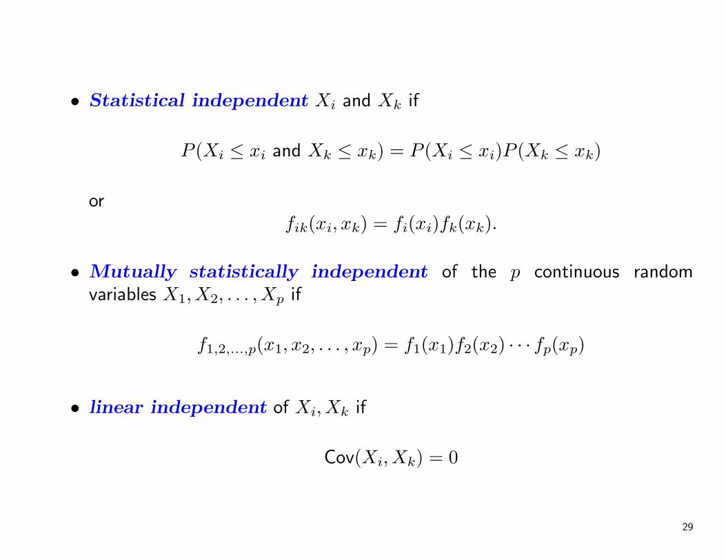
• Statistical independent Xi and Xk if

P (Xi ≤ xi and Xk ≤ xk) = P (Xi ≤ xi)P (Xk ≤ xk)

orfik(xi, xk) = fi(xi)fk(xk).

• Mutually statistically independent of the p continuous randomvariables X1, X2, . . . , Xp if

f1,2,...,p(x1, x2, . . . , xp) = f1(x1)f2(x2) · · · fp(xp)

• linear independent of Xi, Xk if

Cov(Xi, Xk) = 0

29

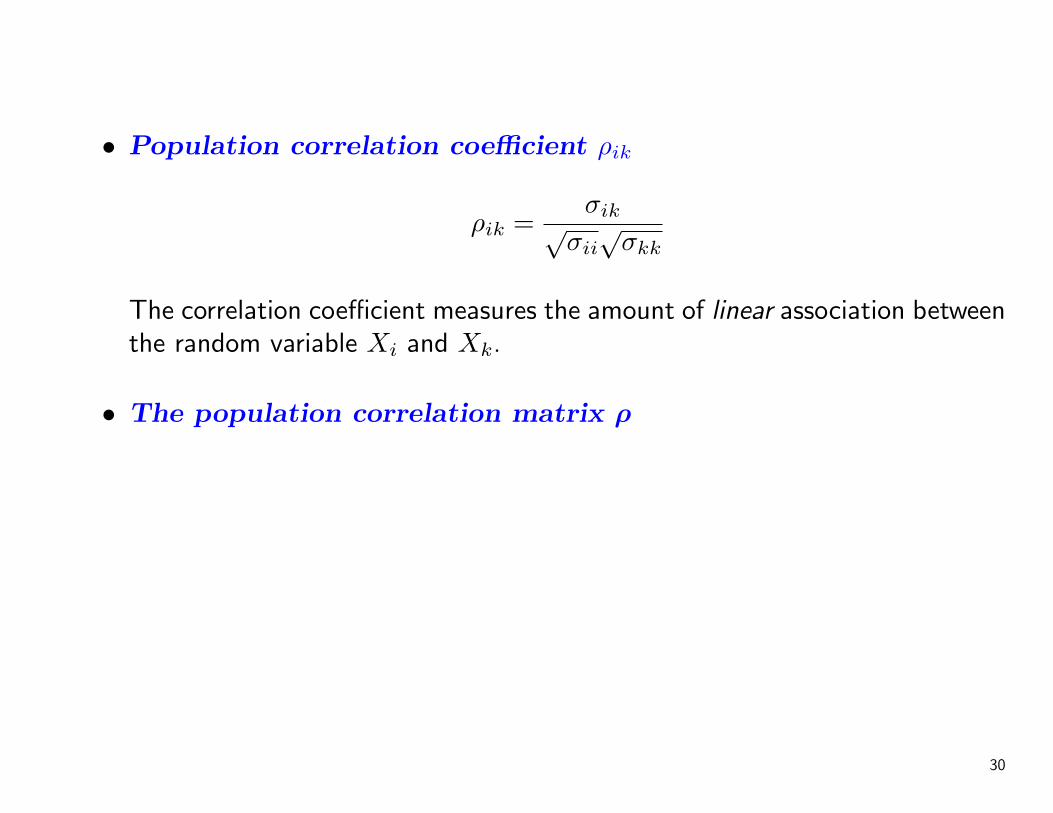
• Population correlation coefficient ρik

ρik =σik√

σii√

σkk

The correlation coefficient measures the amount of linear association betweenthe random variable Xi and Xk.

• The population correlation matrix ρ

30

Example 2.12 (Computing the covariance matrix) Find the covariancematrix for the two random variables X1 andX2 introduced in Example 2.11when their joint probability function p12(x1, x2) is represented by the entries inthe body of the following table:

x1\x2 0 1 p1(x1)-1 0.24 0.06 0.30 0.16 0.14 0.31 0.4 0.00 0.4

p2(x2) 0.8 0.2 1

Example 2.13 (Computing the correlation matrix from the covariancematrix) Suppose

Σ =

4 1 21 9 −32 −3 25

=

σ11 σ12 σ13

σ12 σ22 σ23

σ13 σ23 σ33

Obtain the population correlation matrix ρ

31

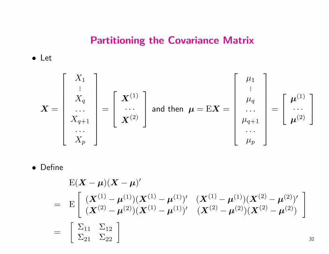
Partitioning the Covariance Matrix

• Let

X =

X1...

Xq

. . .Xq+1

. . .Xp

=

X(1)

· · ·X(2)

and then µ = EX =

µ1...

µq

. . .µq+1

. . .µp

=

µ(1)

· · ·µ(2)

• Define

E(X − µ)(X − µ)′

= E

[(X(1) − µ(1))(X(1) − µ(1))′ (X(1) − µ(1))(X(2) − µ(2))′

(X(2) − µ(2))(X(1) − µ(1))′ (X(2) − µ(2))(X(2) − µ(2))

]

=[

Σ11 Σ12

Σ21 Σ22

]32

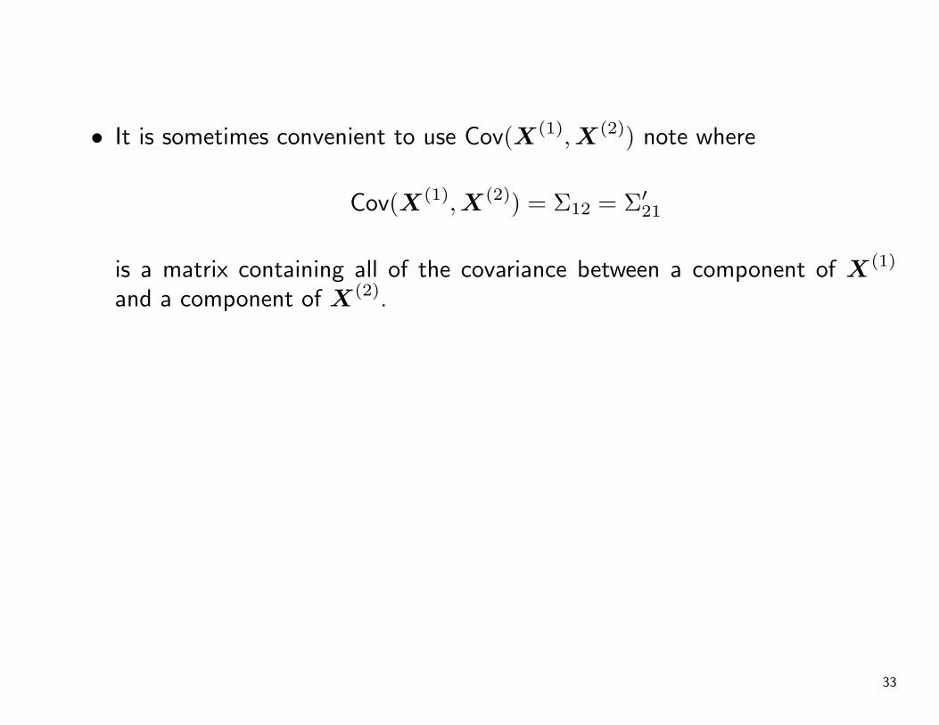
• It is sometimes convenient to use Cov(X(1),X(2)) note where

Cov(X(1),X(2)) = Σ12 = Σ′21

is a matrix containing all of the covariance between a component of X(1)

and a component of X(2).

33

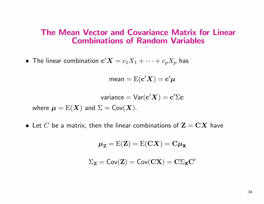
The Mean Vector and Covariance Matrix for LinearCombinations of Random Variables

• The linear combination c′X = c1X1 + · · ·+ cpXp has

mean = E(c′X) = c′µ

variance = Var(c′X) = c′Σc

where µ = E(X) and Σ = Cov(X).

• Let C be a matrix, then the linear combinations of Z = CX have

µZ = E(Z) = E(CX) = Cµx

ΣZ = Cov(Z) = Cov(CX) = CΣxC′

34

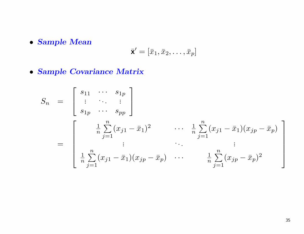
• Sample Meanx̄′ = [x̄1, x̄2, . . . , x̄p]

• Sample Covariance Matrix

Sn =

s11 · · · s1p... . . . ...

s1p · · · spp

=

1n

n∑j=1

(xj1 − x̄1)2 · · · 1n

n∑j=1

(xj1 − x̄1)(xjp − x̄p)

... . . . ...

1n

n∑j=1

(xj1 − x̄1)(xjp − x̄p) · · · 1n

n∑j=1

(xjp − x̄p)2

35

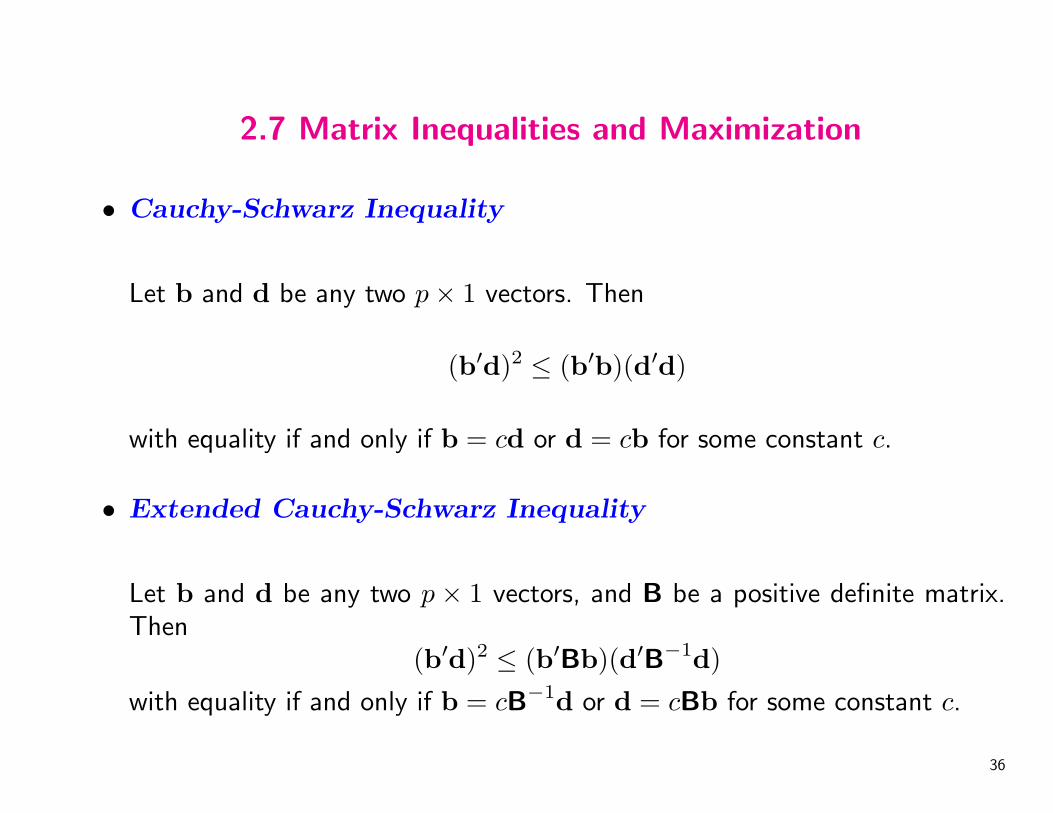
2.7 Matrix Inequalities and Maximization

• Cauchy-Schwarz Inequality

Let b and d be any two p× 1 vectors. Then

(b′d)2 ≤ (b′b)(d′d)

with equality if and only if b = cd or d = cb for some constant c.

• Extended Cauchy-Schwarz Inequality

Let b and d be any two p × 1 vectors, and B be a positive definite matrix.Then

(b′d)2 ≤ (b′Bb)(d′B−1d)

with equality if and only if b = cB−1d or d = cBb for some constant c.

36

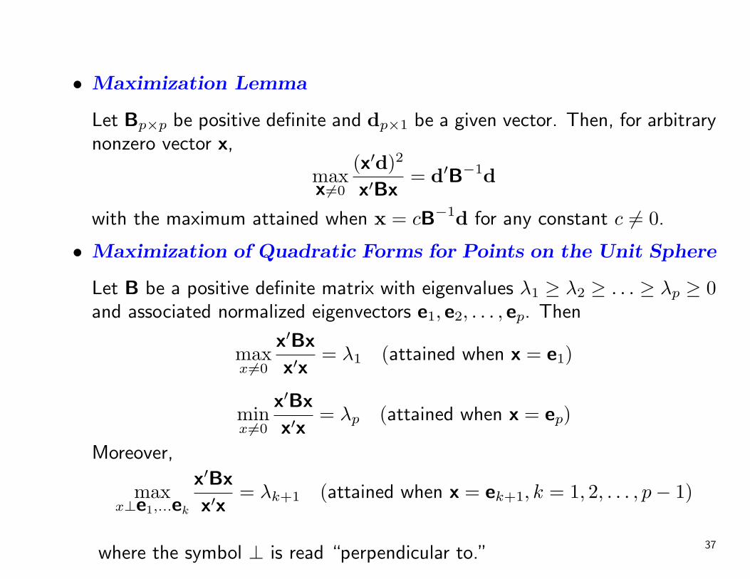
• Maximization Lemma

Let Bp×p be positive definite and dp×1 be a given vector. Then, for arbitrarynonzero vector x,

maxx 6=0

(x′d)2

x′Bx= d′B−1d

with the maximum attained when x = cB−1d for any constant c 6= 0.

• Maximization of Quadratic Forms for Points on the Unit Sphere

Let B be a positive definite matrix with eigenvalues λ1 ≥ λ2 ≥ . . . ≥ λp ≥ 0and associated normalized eigenvectors e1, e2, . . . , ep. Then

maxx6=0

x′Bx

x′x= λ1 (attained when x = e1)

minx6=0

x′Bx

x′x= λp (attained when x = ep)

Moreover,

maxx⊥e1,...ek

x′Bx

x′x= λk+1 (attained when x = ek+1, k = 1, 2, . . . , p− 1)

where the symbol ⊥ is read “perpendicular to.”37