MATR316, Nuclear Physics, 10 cr

Fall 2017, Period II

Pertti O. Tikkanen

Lecture Notes of Tuesday, Nov. 21th and Thursday, Nov. 23th

Department of Physicspertti.tikkanen@helsinki.fi

1

Nuclear Mean Field

Introduction

Hartree-Fock

Measuring the nuclear density distributions: a test of single-particle motion

Hartree-Fock theory: a variational approach

Configuration mixing: model space and model interaction

1

Nuclear Mean Field

We started the nucleon single-particle description

• from a given independent particle picture, i.e.

• assuming that nucleons mainly move independently from each other

• in an average field with a large mean-free path.

However, in the basic non-relativistic approach we have to start from a picture

• where we have A nucleons moving in the nucleus with given kinetic energy(~p 2

i /2mi ) and

• interacting with the two-body force V (i, j).

• Eventually, higher-order interactions V (i, j, k) or density-dependent interactionsmay be considered.

2

• The starting point is the nuclear A-body Hamiltonian

H =A∑

i=1

~p 2i

2mi+

A∑i<j=1

V (~ri ,~rj ), (223)

• which is at variance to the A-independent nuclear Hamiltonian

H0 =A∑

i=1

(~p 2

i

2mi+ U(|~ri |)

)=

A∑i=1

h0(i). (224)

• Denoting all quantum numbers characterizing the single-particle motion by thenotation i ≡ ni , li , ji ,mi we have

h0(i)φi (~r) = εiφi (~r), (225)

• and the A-body, independent particle wavefunction becomes (not taking theanti-symmetrization into account for the moment)

Ψ1,2,...,A(~r1,~r2, . . . ,~rA) =A∏

i=1

φi (~ri ), (226)

• corresponding to the solution of H0 with total eigenvalue E0,

H0Ψ1,2,...,A(~r1,~r2, . . . ,~rA) = E0Ψ1,2,...,A(~r1,~r2, . . . ,~rA) (227)

with

E0 =A∑

i=1

εi .

3

However,

• The wavefunctions φ(~ri ) have been obtained starting from the chosen averagefield U(|~r |)

• It is not guaranteed that this potential will give rise to wavefunctions that minimizethe total energy of the interacting system.

The Hartree-Fock method produces such a wavefunction, by following a simple, butintuitive approach to

• obtain the ‘best’ wavefunctions φHFi (~ri )

• and corresponding energies εHFi

• starting from the knowledge of the two-body interaction V (~ri ,~rj ).

4

Assuming the nucleus to consist of a number of separated point particles at positions~ri

(see figure 35(a)),

• interacting through the two-body potentials V (~ri ,~rj ),

• the total potential acting on a given point particle at~ri is obtained by summing thevarious contributions, i.e.

U(~ri ) =∑

j

V (~ri ,~rj ). (228)

For a continuous distribution, characterized by a density distribution ρ(~r ′),

• the potential energy at point~r is obtained by folding the density with the two-bodyinteraction to give (figure 35(b))

U(~r) =

∫ρ(~r ′)V (~r ,~r ′) d~r ′. (229)

5

Figure 35: (a) A collection of A particles (withcoordinates~ri ), representing an atomic nucleus interms of the individual A nucleons, interacting viaa two-body force between any two nucleons, i.e.V (~ri ,~rj ).(b) The analogous, continuous mass distribution,described by the function ρ(~r). The density at agiven point (in a volume element d~r ) ρ isillustrated pictorially. This density distribution isthen used to determine the average, one bodyfield U(~r)

6

In order to accomplish the above self-consistent study, we have to solve theSchrodinger equation

−~2

2m∇2φi (~r) +

∑b∈F

∫φ∗b (~r ′)V (~r ,~r ′)φb(~r ′)φi (~r)d~r ′ = εiφi (~r), (230)

• for all values of i (i encompasses the occupied orbits b and also the other,unoccupied ones).

• In the Schrödinger equation, we need to take care of the antisymmetrizationbetween the two identical nucleons in orbit b (at point~r ′) and in orbit i (at point~r ).

• The correct equation follows by substituting

φb(~r ′)φi (~r)→[φb(~r ′)φi (~r)− φb(~r)φi (~r ′)

], (231)

and becomes

−~2

2m∇2φi (~r) +

∑b∈F

∫φ∗b (~r ′)V (~r ,~r ′)φb(~r ′) d~r ′ · φi (~r)

−∑b∈F

∫φ∗b (~r ′)V (~r ,~r ′)φb(~r)φi (~r ′) d~r ′ = εiφi (~r). (232)

for i = l, 2, . . . ,A; A + 1, . . .

7

• Using the notation

UH(~r) =∑b∈F

∫φ∗b (~r ′)V (~r ,~r ′)φb(~r ′) d~r ′

UF(~r ,~r ′) =∑b∈F

φ∗b (~r ′)V (~r ,~r ′)φb(~r) (233)

• the Hartree-Fock self-consistent set of equations to be solved becomes − ~2

2m∇2φi (~r) +UH(~r)φi (~r) −

∫UF(~r ,~r ′)φi (~r ′) d~r ′ = εiφi (~r)

......

......

(234)

• Solving the coupled set of integro-differential equations is complicated.

• In particular, the non-local part generated by UF(~r ,~r ′) causes difficulties.

• For zero-range two-body interactions this integral contribution becomes localagain.

8

The procedure to solve the coupled equations:

1. start from initial guesses for the wavefunctions φ(0)i (~r) from which

2. the terms U(0)H (~r) and U(0)

F (~r ,~r ′) could be determined,

3. the solution will then give rise to a first estimate of ε(1)i

4. and the corresponding wavefunctions φ(1)i (~r).

5. Go on with this iterative process until convergence shows up

6. call these solutions φHFi (~r), εHF

i , UHF(~r) (the local and non-local converged one-and two-body quantities (figure 36)).

In order to this make any sense, we need to show that

• with these optimum wavefunctions, the expectation value of the total Hamiltonian⟨Ψ1,2,...,A(~r1,~r2, . . . ,~rA)|H|Ψ1,2,...,A(~r1,~r2, . . . ,~rA)

⟩, (235)

becomes minimal EHF(min),

• when we use the antisymmetrized A-body wavefunctions

Ψ1,2,...,A(~r1,~r2, . . . ,~rA) = AΨ1,2,...,A(~r1,~r2, . . . ,~rA), (236)

where A is an operator which antisymmetrizes the A-body wavefunction and isconstructed from the Hartree-Fock single-particle wavefunctions.

9

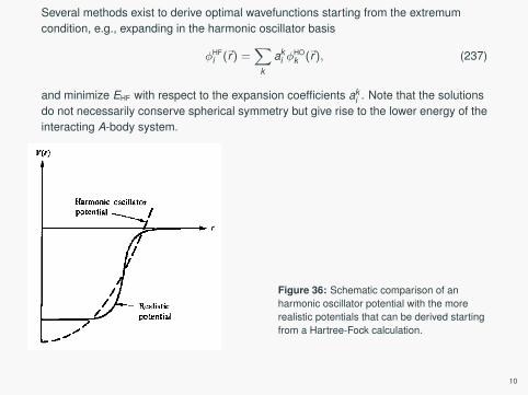
Several methods exist to derive optimal wavefunctions starting from the extremumcondition, e.g., expanding in the harmonic oscillator basis

φHFi (~r) =

∑k

aki φ

HOk (~r), (237)

and minimize EHF with respect to the expansion coefficients aki . Note that the solutions

do not necessarily conserve spherical symmetry but give rise to the lower energy of theinteracting A-body system.

Figure 36: Schematic comparison of anharmonic oscillator potential with the morerealistic potentials that can be derived startingfrom a Hartree-Fock calculation.

10

Once we have determined the Hartree-Fock single-particle orbitals, variousobservables characterizing the nuclear ground-state can be derived:

• nuclear binding energy EHF,

• the various radii (mass, charge) as well as

• the particular charge and mass density distributions.

The nuclear density is given by the sum of the individual single-particle densitiescorresponding to the occupied orbits (if this independent-particle model is to hold to agood degree)

ρ(~r) =∑b∈F

ρb(~r). (238)

See figure 37 for a number of charge density distributions for doubly magic nuclei 16O,40Ca, 48Ca, 90Zr, 132Sn, and 208Pb.

• The theoretical curves have been determined using specific forms ofnucleon-nucleon interaction that are of zero-range in coordinate space (δ(~ri −~rj ))

but are, at the same time, density- and velocity-dependent.

• Such forces are called Skyrme effective interactions.1

• In general, good agreement is observed.

1T.H.R. Skyrme, Phil. Mag. 1 (1956) 1043

11

Figure 37: Charge densities (in units e fm−3) for a number of closed-shell nuclei 16O, 40Ca, 48Ca,90Zr, 132Sn, and 208Pb. The theoretical curves are obtained using effective forces of the Skyrmetype and are compared to the data.

12

• See figure 38 for the various mass density distributions ρm (fm−3) for all of theabove nuclei

• compare these with the nuclear matter value.

• Nuclear matter is a system which is ideal in the sense that no surface effectsoccur, and has a uniform density that approximates to the interior of a heavynucleus with N = Z = A/2.

• In most cases, the electromagnetic force is neglected relative to the strong,nuclear force.

• The equation of state of infinite nuclear matter is under active research.

13

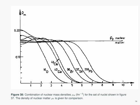
Figure 38: Combination of nuclear mass densities ρm (fm−3) for the set of nuclei shown in figure37. The density of nuclear matter ρF is given for comparison.

14

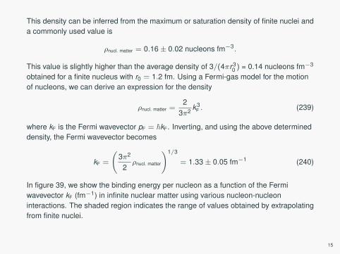
This density can be inferred from the maximum or saturation density of finite nuclei anda commonly used value is

ρnucl. matter = 0.16± 0.02 nucleons fm−3.

This value is slightly higher than the average density of 3/(4πr30 ) = 0.14 nucleons fm−3

obtained for a finite nucleus with r0 = 1.2 fm. Using a Fermi-gas model for the motionof nucleons, we can derive an expression for the density

ρnucl. matter =2

3π2k3

F . (239)

where kF is the Fermi wavevector pF = ~kF. Inverting, and using the above determineddensity, the Fermi wavevector becomes

kF =

(3π2

2ρnucl. matter

)1/3

= 1.33± 0.05 fm−1 (240)

In figure 39, we show the binding energy per nucleon as a function of the Fermiwavevector kF (fm−1) in infinite nuclear matter using various nucleon-nucleoninteractions. The shaded region indicates the range of values obtained by extrapolatingfrom finite nuclei.

15

Figure 39: Binding energy (per nucleon) as afunction of the nucleon Fermi momentum kF ininfinite nuclear matter. The shaded regionrepresents possible values extrapolated fromfinite nuclei. The small squares correspond tovarious calculations with potentials HJ:Hamada-Johnston; BJ: Bethe-Johnson; BG:Bryan-Gersten; SSC: super-soft-core). The solidlines result from various Dirac-Bruecknelcalculations; dashed lines correspond toconventional Brueckner calculations.

16

A very good test of the nuclear single-particle structure in atomic nuclei would bepossible

• if we were to know the densities in a number of adjacent nuclei such thatdifferences determine a single contribution from a given orbital.

• Such a procedure was followed by Cavedon et al (1982) and Frois et al (1983).

• Using electron scattering experiments, the charge density distributions weredetermined in 206Pb and 205Tl.

• From the difference

ρch(206Pb)− ρch(205Tl) =∑b∈F

|φb(~r)|2 (206Pb)−∑

b∈F ′|φb(~r)|2 (205Tl)

= |φ3s1/2(~r)|2, (241)

it should be possible to obtain the structure of the 3s1/2 proton orbit.

• The results are shown in figure 40, and give an unambiguous and sound basis forthe nuclear independent-particle model as a very good description of the nuclearA-body system.

• The method of electron scattering is, in that sense, a very powerful method todetermine nuclear ground-state properties (charge distributions, charge transitionand current transition densities,. . . ).

17

Figure 40: The nuclear density distribution for the least bound proton in 206Pb. The shell modelpredicts the last (3s1/2) proton in 206Pb to have a sharp maximum at the centre, as shown at theleft-hand side. On the right-hand side, the nuclear charge density differenceρch(206Pb)− ρch(205Tl) = |φ3s1/2(~r)|2 is given (taken from Frois (I983) and DOE (1983)).

18

Variational approach to Hartee-Fock theory

The starting point of the Hartree-Fock theory (HF) is the description of the many-bodywave function as an antisymmetrized product of the single-particle wavefunctions(Slater determinant):

Ψ(1, 2, . . . ,A) = Aφα1 (1)φα2 (2) . . . φαA (A), (242)

whereA ≡

∑P

(−1)P P

with P is the permutation operator, permuting the A nucleon coordinates and(−1)P = ±1 depending on whether the permutation is even or odd permutation of theindices 1, 2, . . . ,A. The notation 1, 2, . . . ,A describes all coordinates of the nucleonand α1, α2, . . . denotes all quantum numbers to specify a single-particle nuclear state.

19

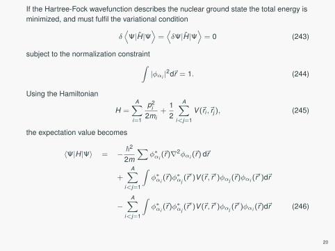
If the Hartree-Fock wavefunction describes the nuclear ground state the total energy isminimized, and must fulfil the variational condition

δ⟨

Ψ|H|Ψ⟩

=⟨δΨ|H|Ψ

⟩= 0 (243)

subject to the normalization constraint∫|φαi |

2d~r = 1. (244)

Using the Hamiltonian

H =A∑

i=1

p2i

2mi+

12

A∑i<j=1

V (~ri ,~rj ), (245)

the expectation value becomes

〈Ψ|H|Ψ〉 = −~2

2m

∑φ∗αi

(~r)∇2φαi (~r) d~r

+A∑

i<j=1

∫φ∗αi

(~r)φ∗αj(~r ′)V (~r ,~r ′)φαj (~r)φαi (~r

′)d~r

−A∑

i<j=1

∫φ∗αi

(~r)φ∗αj(~r ′)V (~r ,~r ′)φαj (~r

′)φαi (~r)d~r (246)

20

Applying the variation on φ∗αi(~r),

∂

∂φ∗αi(~r)

[〈Ψ|H|Ψ〉 −

∑i

εαi

∫|φαi (~r)|2d~r

]= 0 (247)

produces the Schrödinger equation

−~2

2m∇2φαi (~r) +

A∑j=1

∫d~r ′ φ∗αj

(~r ′)V (~r ,~r ′)φαj (~r′)φαi (~r)

−A∑

j=1

∫d~r ′ φ∗αj

(~r ′)V (~r ,~r ′)φαj (~r)φαi (~r′) = εαiφαi (~r) (248)

where εαi is the Lagrange multiplier required for the normalization constrain. It turnsout to be the single-particle energy.

21

Configuration mixing

• In many cases, two valence nucleons outside closed shells

• Several j orbits are possible, none of them can be singled out

• A number of valence shells where the nucleons can move in principle

• As an example, consider 18O with two neutrons outside the 16O core

• In the simplest approach, both move in the energetically most favoured 1d5/2orbit, and only (1d5/2)2, 0+, 2+, 4+ configurations can be formed,

• Our task is to determine the strength of the residual interaction V12 thatreproduces the experimental spacings of 0+, 2+, 4+ levels.

• The next step is to consider the full sd-shell model space with many moreconfigurations for each Jπ :

• For 0+ three possible configurations, (1d5/2)20+ , (2s1/2)2

0+ , and (1d3/2)20+

• Note that the strength of the residual interaction V12 is different in the latter caseof a larger model space, and loosely speaking,

• the larger the model space, the smaller the residual interaction, because in morerealistic models (larger model space) include most of the relevant physics alreadyfrom the beginning and there is no need for phenomenological effectiveinteractions.

22

In the case of 18O, the 1d5/2 and 2s1/2orbits separate from the higher-lying 1d3/2orbit and for our model space we have:

Jπ = 0+ −→ (1d5/2)20+ (2s1/2)2

0+

Jπ = 2+ −→ (1d5/2)22+ (1d5/22s1/2)2+

Jπ = 3+ −→ (1d5/22s1/2)3+

Jπ = 4+ −→ (1d5/2)24+

For example, the energy eigenvalues forthe Jπ states are the correspondingeigenvalues of the Hamiltonian

H = H0 + Hres

=2∑

i=1

h0(i) + V12 (249)

with the core energy (closed shell) E0

taken as a reference.Figure 41: The neutron single-particle energiesin 17O relative to the 1d5/2 orbit, as inferred fromthe experimental spectrum of 17O.

23

Eigenfunctions are linear combinations of the basis functions, and in the case ofJπ = 0+, there are two possibilities:

|Ψ0+;1⟩

=n∑

i=0

ak ;1 |ψ(0)k ; 0+

⟩

=n∑

i=0

ak ;2 |ψ(0)k ; 0+

⟩. (250)

For the particular case of 18O, we thus define

|ψ(0)1 ; 0+

⟩≡ |(1d5/2)2; 0+

⟩|ψ(0)

2 ; 0+⟩≡ |(2s1/2)2; 0+

⟩

24

Before proceeding with this special case, review the general formalism in some depth.

• Let the total wavefunction be expanded in terms of the basis functions:

|Ψp〉 =n∑

k=1

akp |ψ(0)k

⟩. (251)

• With the Hamiltonian of Eq. (249), the Schrödinger equation yields

(H0 + Hres)n∑

k=1

akp |ψ(0)k

⟩= Ep

n∑k=1

akp |ψ(0)k

⟩(252)

⇒n∑

k=1

⟨ψ

(0)l |H0 + Hres|ψ(0)

k

⟩= Epalp, (253)

where Ep are the energies (eigenvalues of the total Hamiltonian).

• Defining the elements of the n × n matrix by

Hlk ≡ E (0)k δlk +

⟨ψ

(0)l |Hres|ψ(0)

k

⟩, (254)

25

• we thus have a set of linear equations

n∑k=1

Hlk akp = Epalp (255)

that has a unique solution if and only if det[H− EpI] = 0

• We are thus faced with finding the n zeros of the characteristic equation:∣∣∣∣∣∣∣∣∣∣H11 − Ep H12 . . . H1n

H21 H22 − Ep . . . H2n...

......

Hn1 − Ep . . . Hnn − Ep

∣∣∣∣∣∣∣∣∣∣= 0 (256)

that occur at the eigenvalues Ep (p = 1, 2, . . . , n).

• The coefficients aik are then determined by substituting each eigenvalue to Eq.(255) and imposing normalization on the final wavefunctions

n∑k=1

apk akp′ = δpp′ (257)

26

• The dimension of the diagonalization problem increases dramatically when moresingle-particle orbits are included in the model space.

• Usually only the few lowest energies (smallest eigenvalues) are of interest and theLanczos algorithm is employed.

• If the non-diagonal matrix elements |Hi 6=j | are of the same order as the

unperturbed energy difference |E (0)i − E (0)

j | large configuration mixing results and

the energies Ep differ considerably from the unperturbed values E (0)k .

• On the other hand, if |Hi 6=j | � |E(0)i − E (0)

j |, the energy shifts are small and evena perturbation approach might suffice.

• The presented formalism can be applied in studying various mixing situations, e.g.for testing the isospin mixing etc.

• In the following, we apply the general results in the case where only two orbits aremixed by the interaction.

• Playing with the two-level toy problem familiarizes us with all the essential featuresthat are present in the more complicated problems of configuration mixing.

• See also the 2014 Talent lectures by R. Casten

27