Embed Size (px)
Citation preview

MATLENG 330
Materials and Processes
in Manufacturing
Lab Manual
Dr. Nidal Abu-Zahra

2
Contents:
1. Statistical Process Control (SPC).........................................................................................3
2. Properties of Cast Materials .................................................................................................9
3. Formability of Sheet Metals...............................................................................................17
4. Ring Compression Test ......................................................................................................21
5. Open Die Forging ..............................................................................................................24
6. Foam Extrusion ..................................................................................................................29
7. Polymer Rheology...…...…...………………………....……….………………..…....….32
8. Polyurethane Foam Casting……………………………………………………………....37
9. Injection Molding…………………………………..…………………………………….42
10. Differential Scanning Calorimetry…………..………………………...…………...…….45
Appendix A: Sample of Scientific Writing……………………………………………..……46

3
Statistical Process Control (SPC)
Objective
1. Determine if a process is “in control”.
2. Determine if a process is within specifications
3. Identify reasons for variation
References
Kalpakjian & Schmid, Manufacturing Processes for Engineering Materials (fifth edition)
Section 1.9 pgs 22-24
Section 4.9.0-2 pgs 175-182
Introduction:
SPC (Statistical Process Control) is a systematic approach to guide operators and manufacturers
in monitoring a process during its operation in order to control the quality of the products while
they are being produced – rather than relying on inspection to find problems after the fact.
SPC is often the first step in a comprehensive quality improvement program is an integral part of
Total Quality Management (TQM) which does not focus on the properties of the final product,
but on the process of production. This means quality is built into the product beginning with the
design and materials chosen, then all subsequent stages of production including assembly and
service. The guiding philosophy of TQM is keeping the process under control and therefore if
the process to manufacture a product is under control then the products are being produced
within specifications.
Using SPC methods engineers can:
Identify critical problem areas
Reduce variation and monitor for unusual variation
Determine the capability of the production process
Understand and optimize the production process
Determine the reliability of the product
As the name implies this process makes use of Statistical Methods. Among these are the
concepts of Sampling and Descriptive Statistics.
Sampling
1. A portion – consecutive, randomly taken samples of a given size - of the entire
population is tested.
2. Testing the whole population is not usually practical and the actual distribution of most
often unknown.
3. Results from the samples are assumed to represent the entire population. (i.e. What
happened to the samples is what we can expect happened to the entire population.)
4. According the Central Limit Theorem the sample averages follows a standard
distribution.

4
Concepts from Descriptive Statistics
The following formulas and concepts are necessary to analyze the data to be collected in the
lab.
Statistic Formula Description / MS-Excel Sample Formula
Average
n
x
x
n
i
i 1
Arithmetic Mean of sampled points
=AVERAGE(A2:C2)
Range R = xmax - xmin A measure of the variation equal to the maximum
measured value minus the minimum measured
value
=MAX(A2:C2)-MIN(A2:C2)
Average
Range
n
R
R
n
i
i 1
Arithmetic Mean of all Range values (from
calculation above)
=AVERAGE(E2:E37)
Standard
Deviation
1
)(1
2
n
xxn
i
i
Another measure of variation based on the
difference of each point from the sample average
=STDEV(D2:D37)
Graphs & Charts:
Histogram: A bar graph which shows the number of occurrences of a particular value versus the
measured value. Below is a histogram created for a sample of measured drive shaft
diameters (from textbook page 177).
Diameter of Shafts (mm)
From this chart it can be seen that measured diameter which occurred most frequently
was 13 mm. Note that on this histogram a normal distribution curve has been
superimposed. Many times the data being measured will conform to this curve. A
normal curve is shown below.

5
In a “Normal Distribution” curve (a.k.a. Bell Curve) the average of all values is mapped
to the zero point of the graph. The scale of the X-Axis of the curve is in dimensions of
Standard Deviations (σ). It has been determined that within a given range a certain
percentage of points will fall within that range and a certain percentage will fall outside
of the range. This is shown for 3 ranges below:
Range
% of Values Inside the Range
% of Values Outside the Range
1x 68.28% 31.72%
2x 95.46% 4.54%
3x 99.73% 0.27%
For the processes studied in this experiment, we will consider 3x to be the range of
values where the process is "in control”. Thus these are the Control Limits. There is the
Upper Control Limit (UCL) and the Lower Control Limit (LCL). The Control Limit
values can also be determined without the standard deviations by using the values of A2,
D3, and D4 which can be looked up in the following table (Table 4.3 from the Textbook
page 180) Sample
Size A2 D4 D3
2 1.880 3.267 0
3 1.023 2.575 0
4 0.729 2.282 0
5 0.577 2.115 0
6 0.483 2.004 0
7 0.419 1.924 0.078
8 0.373 1.864 0.136
9 0.337 1.816 0.184
10 0.308 1.777 0.223
12 0.266 1.716 0.284
15 0.223 1.652 0.348
20 0.180 1.586 0.414

6
As can be seen these values depend on the sample size. The sample size is the number of
measurements taken in order to make a single point for a process control chart. In this
experiment 3 measurements will be used to determine the value of a single point.
Sample Averages Control Chart: To create a Sample Averages Control Chart we measure the parameter of the individual
members of the sample and calculate the average. Then
1. Plot Sample Averages in the order in which they were collected.
2. Plot the Average of the Averages
3. Plot the Upper Control Limit: RAxxUCLx 23
4. Plot the Lower Control Limit: RAxxLCLx 23
Sample Ranges Control Chart: A sample Range Control Chart is constructed as follows:
1. Plot Sample Ranges in the order in which they were collected.
2. Plot the Average of the Ranges
3. Plot the Upper Control Limit: RDUCLR 4
4. Plot the Lower Control Limit: RDLCLR 3

7
Patterns:
We will define a pattern as recurring values in a certain range when the probability of
recurrence is less than 1%.
To determine how many points constitute a pattern for a certain range, we use the Normal
Distribution information presented above.
The probability of finding a single point in the 2x to 3x range is
(99.73%-95.46%) / 2 = 2.14%
The probability of finding 2 points in this range is
2.14% * 2.14% = 0.05%
This is less than 1%. So, finding 2 points in this range constitutes a pattern.
Similar calculations can be performed for other ranges to determine the probability of
recurrence
Procedure:
1. Samples of 1045 steel will be heated in a furnace at 870oC prior to the class.
2. Open the furnace door and quickly remove a sample at a time using tongs and quench it
in a bucket of cold water stirring the water with the sample for several seconds.
3. Close the furnace door and allow the temperature to rise to 870oC again before removing
the next sample.
4. After quenching 3 samples replace the water in the bucket. Repeat procedure for the rest
of the samples.
5. The surface of the samples should be ground on a rough sandpaper (using a grinding
wheel if available) to remove the brittle oxide coating.
6. Measure & record the Rockwell C Hardness (HRC) value for each sample.
Results:
1. Table of Hardness Values – must include: x and Range
2. Table of values calculated for Control Charts – must include x ,σ, R , A2, D3, D4, x
UCL ,
xLCL ,
RUCL ,
RLCL .

8
3. Histogram for HRC (Frequency vs. HRC – no legend necessary, make sure axis labels are
“Frequency” and “HRC”).
[This can be created in MS-Excel automatically: click "Tools" then click "Data Analysis"
then select "Histogram" and click "OK". When the Histogram Dialog Box comes up, click
the "Help” Button for directions.]
4. HRC Sample Control Chart (HRC vs. Sample Number) – legend and chart should
includex
UCL , x
LCL , and x .
5. HRC Range Control Chart (Range vs. Sample Number) – legend and chart should
includeR
UCL , R
UCL , and R .

9
Properties of Cast Materials
Objective
1. To conduct uniaxial tension testing of various materials.
2. To observe tensile deformation and failure.
3. To construct and interpret stress/strain curves.
4. To describe features of fracture surfaces
References
Kalpakjian & Schmid, Manufacturing Processes for Engineering Materials (fifth edition)
Section 2.0.0-2.2.3 pgs 29-38
Section 5.6.0-2 pgs 208-214
Introduction:
Carbon Steels:
Carbon steels contain only carbon as the principal alloying element. Other elements are present
in small quantities, including those added for deoxidation. Silicon and manganese in cast carbon
steels typically range from 0.25 to about 0.80% Si, and 0.50 to about 1.00% Mn.
Carbon steels can be classified according to their carbon content into three broad groups:
Low-carbon steels: <0.20% C
Medium-carbon steels: 0.20 to 0.50% C
High-carbon steels: > 0.50% C
Low-alloy steels contain alloying elements, in addition to carbon, up to a total alloy content of
8%. Other components include Manganese (Mn), Silicon (Si), Chromium (Cr), Molybdenum
(Mo), Vanadium (V), Nickel (Ni), and Copper (Cu). Cast steels containing more than the
following amounts of a single alloying element are considered low-alloy cast steels:
Element Mn Si Ni Cu Cr Mo V W
Amount (%) 1.00 0.80 0.50 0.50 0.25 0.10 0.05 0.05
For deoxidation of carbon and low-alloy steels, aluminum, titanium, and zirconium are used.
Aluminum is more frequently used because of its effectiveness and low cost. Unless otherwise
specified, the normal sulphur limit for carbon and low-alloy steels is 0.06%, and the normal
phosphorus limit is 0.05%.
The concept of carbon equivalent (CE) was introduced to convert into equivalent carbon content
the effect of other elements known to increase the hardness of steel. The AWS definition of CE
is:
155
)(
6
)( CuNiVMoCrSiMnCCE
where C is the % carbon, Mn is the % Manganese, etc.
If strength increases, hardness increases, ductility decreases, and weldability decreases. If CE is
high, say 0.4 to 0.5, then the potential for cracking in welded connections is increased.

10
Carbon steel castings can be produced with a great variety of properties because composition and
heat treatment can be selected to achieve specific combinations of properties, including hardness,
strength, ductility, fatigue resistance, and toughness.
Cast Irons:
The term "cast iron" designates an entire family of metals with a wide variety of properties. It is
a generic term like steel which also designates a family of metals. Steels and cast irons are both
primarily iron with carbon as the main alloying element. Steels contain less than 2% and usually
less than 1% carbon, while all cast irons contain more than 2% carbon. About 2% is the
maximum carbon content at which iron can solidify as a single phase alloy with all of the carbon
in solution in austenite. Thus, the cast irons by definition solidify as heterogeneous alloys and
always have more than one constituent in their microstructure.
In addition to carbon, cast irons must also contain appreciable silicon, usually from 1-3%, and
thus they are actually iron-carbon-silicon alloys. The high carbon content and the silicon in cast
irons make them excellent casting alloys. Their melting temperatures are appreciably lower than
for steel. Molten iron is more fluid than molten steel and less reactive with molding materials.
Formation of lower density graphite in the iron during solidification reduces the change in
volume of the metal from liquid to solid and makes production of more complex castings
possible. Cast irons, however, do not have sufficient ductility to be rolled or forged.
The various types of cast iron cannot be designated by chemical composition because of
similarities between types. Table 1 lists typical composition ranges for the most frequently
determined elements in the five generic types of cast iron. There is a sixth classification for
commercial purposes, the high-alloy irons. These have a very wide range in base composition
and also contain major quantities of other elements.
A very important influence on the properties of gray iron is the effective thickness of the section
in which it is cast. The thicker the metal in the casting and the more compact the casting, the
slower the liquid metal will solidify and cool in the mold. As with all metals, slower
solidification causes a larger grain size to form during solidification. In gray iron, slower
solidification produces a larger graphite flake size. The cooling of a casting from red heat is in
effect a heat treatment. A slower cooling of the casting will produce a lower hardness in the
metallic matrix.
Alternately, iron that is cast into a section that is too thin will solidify very rapidly and can be file
hard. A casting with separate sections that are appreciably different in thickness can have
differences in graphite size and matrix hardness between the thick and thin sections even though
the entire casting was poured with the same iron. These differences in structure produce
differences in mechanical properties.
The addition of 0.5% Mg will produce ductile cast iron. The magnesium causes the graphite to
form spheres, also known as nodules, instead of the usual flakes. This leads to greatly increased
tensile strength.
White cast iron, which is hard, brittle, and not weldable can be annealed to become malleable
cast iron which can be welded, machined, is ductile, and offers good strength and shock
resistance. The long slow cooling of the white ductile iron during annealing forms nodules of
carbon through the breakdown of hard and brittle cementite (Fe3C).

11
Table 1. Range of Compositions for Typical Unalloyed Cast Irons
Percent (%)
Type of Iron Carbon Silicon Manganese Sulfur Phosphorous
White 1.8-3.6 0.5-1.9 0.25-0.8 0.06-0.2 0.06-0.2
Malleable
(Cast White)
2.2-2.9 0.9-1.9 0.15-1.2 0.02-0.2 0.02-0.2
Gray 2.5-4.0 1.0-3.0 0.2-1.0 0.02-0.25 0.02-1.0
Ductile 3.0-4.0 1.8-2.8 0.1-1.0 0.01-0.03 0.01-0.1
Compacted
Graphite
2.5-4.0 1.0-3.0 0.2-1.0 0.01-0.03 0.01-0.1
Figure 1: Typical microstructure of (A) gray iron (100x), graphite flakes in a matrix of 20% free
ferrite (light constituent)and 80% pearlite (dark constituent)(B) white iron (400x), eutectic
carbide (light constituent) plus pearlite (dark constituent), (C) ductile iron (100x), graphite
nodules encased in envelopes in a matrix of free ferrite, all in a matrix of ferrite, (D) malleable
iron (100x), graphite nodules in a matrix of ferrite.
The presence of certain minor elements is also vital to the successful production of each type of
iron. For example, nucleating agents, called inoculants, are used in the production of gray iron to
control the graphite type and size. Trace amounts of bismuth and tellurium are used in the
production of malleable iron, and the presence of a few hundredths of a percent magnesium
causes the formation of the spherulitic graphite in ductile iron.
In addition, the composition of an iron must be adjusted to suit particular castings. Small castings
and large castings of the same grade of iron cannot be made from the same composition of metal.
For this reason most iron castings are purchased on the basis of mechanical properties rather than
composition. The common exception is for castings that require special properties such as
corrosion resistance or elevated temperature strength.
A B
C D

12
The various types of cast iron can be classified by their microstructure. This classification is
based on the form and shape in which the major portion of the carbon occurs in the iron. This
system provides for five basic types: white iron, malleable iron, gray iron, ductile iron and
compacted graphite iron. Each of these types may be moderately alloyed or heat treated without
changing its basic classification. The high-alloy irons, generally containing over 3% of added
alloy, can also be individually classified as white, gray or ductile iron, but the high-alloy irons
are classified commercially as a separate group.
The wide spectrum of properties of cast iron is controlled by 3 main factors:
1 the chemical composition of the iron;
2 the rate of cooling of the casting in the mould (which depends in part on the section
thicknesses in the casting);
3 the type of graphite formed (if any).
Cast irons may often be used in place of steel at considerable cost savings. The design and
production advantages of cast iron include
1. low tooling and production cost
2. ready availability
3. good machinability without burring
4. readily cast into complex shapes
5. excellent wear resistance and high hardness (particularly white irons)
6. high inherent damping
A good website which explains cast irons is:
http://www.tech.purdue.edu/met/courses/met141/WKD's Lect pp notes-f01/284-CI-NF.ppt
Aluminum:
About 20% of all aluminum is used as castings. The most common casting processes are sand
casting; permanent mold casting and pressure die casting.
There are several advantages of aluminum castings including the light weight of the metal,
recyclability, relatively low melting temperatures, negligible solubility for most gases (with the
exception of H2), good surface finishes are achievable, and the molten metal has good fluidity.
Disadvantages of aluminum castings include relatively high solidification shrinkage (3.5-8.5%),
pressure die cast products are susceptible to air blistering during solution (heat treatments), the
possibility of distortion due to stress relief during heating, and the mechanical properties are
inferior to wrought products
It is important when casting aluminum to control impurity levels and grain size.
The United States Aluminum Association has developed a 4 digit system to classify alloys into
groups. The following is only the first digit which specifies the alloy group.
# 1XX.X PURE ALUMINUM (>99%)
# 2XX.X ALUMINUM-COPPER
# 3XX.X ALUMINUM-SILICON (+ COPPER &/OR MAGNESIUM)
# 4XX.X ALUMINUM-SILICON
# 5XX.X ALUMINUM-MAGNESIUM
# 6XX.X UNUSED
13
# 7XX.X ALUMINUM-ZINC
# 8XX.X ALUMINUM-TIN
# 9XX.X ALUMINUM-OTHER ELEMENTS
Brass:
The copper alloys may be endowed with a wide range of properties by varying their composition
and the mechanical and heat treatment to which they are subjected.
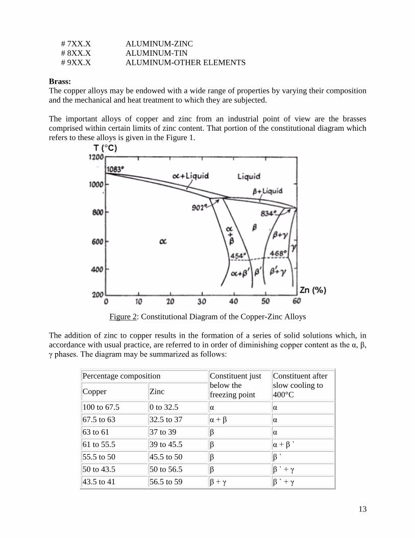
The important alloys of copper and zinc from an industrial point of view are the brasses
comprised within certain limits of zinc content. That portion of the constitutional diagram which
refers to these alloys is given in the Figure 1.
Figure 2: Constitutional Diagram of the Copper-Zinc Alloys
The addition of zinc to copper results in the formation of a series of solid solutions which, in
accordance with usual practice, are referred to in order of diminishing copper content as the α, β,
γ phases. The diagram may be summarized as follows:
Percentage composition Constituent just
below the
freezing point
Constituent after
slow cooling to
400°C Copper Zinc
100 to 67.5 0 to 32.5 α α
67.5 to 63 32.5 to 37 α + β α
63 to 61 37 to 39 β α
61 to 55.5 39 to 45.5 β α + β `
55.5 to 50 45.5 to 50 β β `
50 to 43.5 50 to 56.5 β β ` + γ
43.5 to 41 56.5 to 59 β + γ β ` + γ

14
Further changes in composition of the α and β phases below 400°C are only observed after
prolonged annealing.
There is a certain connection between the properties and the microstructure which may be
expressed in general terms.
The tensile strength increases with increase in zinc content, rises somewhat abruptly with the
appearance of β, and reaches a maximum at a composition corresponding roughly to equal parts
of α and β. It falls off rapidly at the appearance of the γ phase.
Elongation rises to a maximum and begins to fall again before the composition reaches the limit
of the α solution. It falls considerably as the amount of β increases, and is very small in the
presence of γ.
The α phase shows the greatest resistance to shock. This is diminished by the presence of β, and
the alloy becomes extremely brittle when γ is present.
Hardness is greatly increased by the presence of β and still further when γ appears.
Alloys containing α phase only are especially suitable for cold working, and may be hot or cold
rolled. Those containing α and b will suffer very little deformation without rupture in the cold
rolling and may only be hot rolled. The β phase may also be forged, rolled or hot extruded, but
alloys containing γ should invariably be avoided for any mechanical treatment.
It is a frequent procedure in casting brass to draw it into rod to employ very long moulds of very
small cross section, in order to minimize subsequent mechanical treatment.
Tensile Stress-Strain Curves:
Important information about how a material behaves when subjected to tensile stresses can be
obtained when a plot of applied stress versus strain is created. An example stress-strain curve is
shown below in which the engineering stress is plotted against the engineering strain.
The engineering stress, σ, assumes that the cross-sectional area of the sample being stressed in
tension does not change and therefore σ = P/Ao where P is the applied force and Ao is the initial
cross-sectional area of the sample.
The engineering strain, ε, assumes that changes to the length of the sample are so small
compared to the length of the sample that they can be ignored and thus only the original length of
the sample needs to be considered. The engineering strain is defined as ε = (li-lo)/lo or ε = Δl / lo.
The engineering stress and strain are valid only for small stresses and strains in which the
material deforms elastically.

15
Figure 3: Engineering Stress-Strain Curve
Figure 4: True Stress-Strain Curve
As can be seen for small strains the stress-strain curve is linear. This area of the curve is known
as the elastic region. In this region the material behaves as a spring in that when the stress is
removed, the material will return to its original shape and dimensions. The slope of the line, E,
is called the Young’s Modulus of Elasticity (which is usually shortened to Young’s Modulus or
Elastic Modulus). The stress, σ, and strain, ε, are proportional to each other. The relationship
can be expressed as E = /.
Also clear in the sample curve is a region in which the stress and strain are no longer linear. This
is known as the plastic region. In this region, the material deforms plastically. This means that
when the stress is removed, the elastic energy will be released, but the sample will no longer
return completely to its original dimensions.
The stress at which the behavior of the material changes from elastic to plastic is called the yield
stress, σy. This stress is often determined using the 0.2% offset method. In this method, a line is
drawn with an origin at σ = 0 and ε = 0.002 (i.e. 0.2%) and has the same slope, E, as the Young’s
Modulus of Elasticity of the material. Thus it will intercept the stress-strain curve at some point
in the plastic region where the curve begins to flatten out. The intercept point defines the yield
point. The stress at this point is the yield stress, σy.

16
Above the yield point, the material no longer has a linear stress-strain relationship. In fact the
behavior of the material can be described as σt=Kεtn. The factor n is called the Strain
Hardening Coefficient.
In this area the assumptions necessary for the engineering stress and engineering strain are no
longer valid. This is because the cross-sectional area of the sample will begin to decrease. This
decrease or “necking” will become very pronounced in a certain area of the sample which
eventually leads to failure. The stress at which the necking becomes noticeable can be seen as
the highest stress achieved in the stress-strain curve. This is known as the Ultimate Tensile
Strength or UTS.
To truly describe the stress and strain in the material when it is subjected to stresses in the plastic
region it is necessary to determine the true stress and true strain. These do not rely on the
assumptions of the engineering stress and strain, but depend on the instantaneous cross-sectional
area and instantaneous change in length of the sample. Thus they are defined as σt = P/Ai and
εt = δl / l = ln (li/lo) = ln(Ao/Ai). Note: εt is sometimes designated as “e”.
These instantaneous values are difficult to measure while conducting tests. However, they can
be calculated from the engineering stress and engineering strain based on the assumption that the
volume of the sample will remain constant throughout the test.
Therefore εt = ln(ε + 1) and σt = σ(ε + 1).
The strain hardening coefficient, n, is found using the true stress and true strain.
To find it, a plot of log (σt) vs log (εt) is created for values of stress and strain between the yield
stress, σy, and the UTS.
The true stress-strain curve on a logarithmic scale should be approximately linear. Therefore the
slope of the line is the value of the strain hardening coefficient, n.
Procedure:
Use the SATEC universal testing machine to tensile test the five samples.
1. 1045 steel cast sample
2. gray cast iron sample
3. ductile cast iron sample
4. aluminum sample
5. brass sample
Note: more accurate results will be obtained for strain if an extensometer is used.
Results:
1. Plot engineering stress-strain curves for each of the 5 samples (in Excel, turn off dots
otherwise the lines will be too thick)
2. From the data determine the Young’s Modulus of Elasticity for each material
3. From the data determine the Yield Stress of each material
4. From the data determine the UTS of each material
5. From the data determine the Strain Hardening Exponent, n, for each material.
(Remember that the engineering stress and strain must be converted to the true stress and strain
and the slope of the log σt vs log εt plot between the Yield Stress and the UTS will be the value
of n.
6. From the data determine strain to fracture.
7. Compare the experimental values to expected values from the text.

17
Formability of Sheet Metals
Objective
1. To conduct tension testing of various sheet metals.
2. To observe the effect of grain orientation
3. To observe tensile deformation
4. To evaluate major and minor strains
5. To construct and interpret the forming-limit diagram
References
Kalpakjian & Schmid, Manufacturing Processes for Engineering Materials (fifth edition)
Section 7.7.0-3 pgs 387-403
Introduction:
Sheet-Metal Characteristics
Sheet metals are generally characterized by a high ratio of surface area to thickness. Forming of
sheet metals is usually carried out by tensile forces in the plane of the sheet; otherwise the
application of compressive forces could lead to buckling, folding, and wrinkling of the sheet.
Unlike bulk deformation processes, in most sheet-forming processes any thickness change is
caused by stretching of the sheet under tensile stresses (Poissons ratio). This decrease in
thickness should be avoided in most cases since it can lead to necking and failure. The major
factors that significantly influence the overall sheet-forming operation are:
Elongation:
A specimen subjected to tension first undergoes uniform elongation that corresponds to the
ultimate tensile strength. Then necking begins and nonuniform elongation occurs until
fracture takes place. The material is being stretched in sheet forming, so high uniform
elongation is desirable for good formability.
Yield-point elongation
Low-carbon steels exhibit this behavior, which indicates that after the material yields, it
stretches farther in certain regions in the specimen with no increase in the lower yield point,
while other regions have not yet yielded. This behavior produces Lueders bands (or stretcher
strain marks or worms) on the sheet, making elongated depressions on the surface of the
sheet. To avoid this problem, the thickness of the sheet is reduced by 0.5 to 1.5% by cold
rolling.
Anisotropy
Anisotropy is the directionality of the sheet metal. It is acquired during the heat treating and
deforming of the sheet. There are two types of anisotropy: crystallographic anisotropy (from
preferred grain orientation) and mechanical fibering (from alignment of impurities,
inclusions, voids, and the like, throughout the thickness of the sheet during
processing).Anisotropy may be present in both the plane of the sheet and its thickness
direction.
Grain size
The grain size is important because it affects the mechanical properties of the material and
the surface appearance of the formed part. The coarser the grain, the rougher will be the
surface.

18
Residual stresses
Residual stresses can be present in sheet metal parts because of the nonuniform deformation
of the sheet during forming. When disturbed, such as by removing a portion of it, the part
may distort. Tensile residual stresses on surfaces can also lead to stress-corrosion cracking of
sheet-metal parts unless they are properly stress relieved.
Springback
Sheet-metal parts are generally thin and are subjected to relatively small strains. Thus they
are likely to experience considerable springback, particularly in bending and other sheet-
forming operations where the bend radius-to-thickness ratio is high. The stress distribution in
a bended material, independent of the thickness of the material or other parameters, shows
tension in the outer fibers and compression in the inner fibers as well as a neutral zone in
which the stress is zero. Therefore, there are fibers in the bend sheet which are only exposed
to a stress level in the elastic region and because these are not permanently deformed this
causes the springback. In order to compensate the sheet can be either over bend or a
stretching operation can be applied in which a tensile stress above yield strength is applied to
the total cross section.
Wrinkling
Although the sheet metal is generally subjected to tensile stresses, the method of forming
(especially bending) may cause compressive stresses to develop in the plane of the sheet,
which cause wrinkling, buckling, folding, or collapsing of the sheet. The tendency for
wrinkling increases with the unsupported or unconstrained length or surface area of the sheet,
decreasing thickness, and non-uniformity of the thickness.
Coated sheet metal
Sheet metals, especially steel, pre-coated with a variety of organic coatings, films, and
laminates are available and used primarily for appearance and corrosion resistance. Coating
is applied to the coil stock on continuous lines, with thickness ranging from 0.0025 to 0.2
mm on flat surfaces.
Formability of Sheet Metals
Sheet-metal formability is defined as the ability of the metal to undergo the desired shape
changes without failures such as nicking and tearing. Three factors have a major influence on
formability:
1. Properties of the sheet metal
2. Lubrication at various interfaces between the sheet and dies and tooling
3. Characteristics of the equipment and tools and dies
Several techniques have been developed to test the formability of sheet metals.
Testing for formability:
1. Tensile test. The tensile test is the most basic and common test used to evaluate
formability. Important properties are determined, such as total elongation of the sheet
specimen at fracture, the strain hardening exponent n, the planar anisotropy, and the normal
anisotropy R of the sheet.
2. Cupping test. Because sheet forming is basically a biaxial stretching process, the earliest
tests developed to determine or to predict formability were cupping test, such as the
Erichsen and Olsen tests (stretching) and the Swift an Fukui tests (drawing). A typical
cupping test is the Erichsen test. The sheet metal specimen is clamped over a circular flat
die with a load of 1000 kg. A 20 mm diameter steel ball is then hydraulically pushed into

19
the sheet metal until a crack appears on the stretched specimen or the punch force reaches a
maximum. The distance d, in millimeters, is the Erichsen number. The greater the value of
d, the greater is the formability of the sheet. Cupping tests measure the capability of the
material to be stretched before fracturing and are relatively easy to perform. However they
not simulate the exact conditions of actual forming operations, because the stretching under
a ball is axisymmetric.
3. Bulge test. Equal (balanced) biaxial stretching of the sheet metals is also performed in the
bulge test, which has been used extensively to simulate sheet-forming operations. In this
test, a circular blank is clamped at its periphery and is bulged by hydraulic pressure, thus
replacing the punch. The process is one of pure stretch forming, and no friction is involved,
as in using the punch. This test can be used to provide effective stress-effective strain
curves for biaxial loading under frictionless conditions. The biaxial bulge limit is also a
sensitive measure.
An important development in testing formability of sheet metals is the construction of forming-
limit diagrams (FLD). The FLD for various sheet metals is shown below. The region above the
curves is the failure zone; R is the normal anisotropy.
Figure 1: Forming Limit Diagram (from textbook page 399)
The curve for each material is created by testing in different states of strain. Using the tensile
test, this can be accomplished by testing samples of various widths until near the UTS.
From the graph, it can be seen that different materials have different forming-limit diagrams. The
higher the curve, the better is the formability. In addition, it is desirable for the minor strain to be
negative, i.e. shrinking in the minor direction. In fact, special tools have been designed for
forming sheet metals that take advantage of this effect.
Sheet metal thickness affects the FLD also. The thicker the sheet, the higher its formability
curve. However, in actual operation, thick blank may not bend as easily around small radii. The
rate of deformation on FLD should be assessed for each material as well. Extensive studies are
being carried out to develop new test methods to predict the behavior of metals in sheet-forming
processes.

20
Samples:
5052 aluminum alloy (2.5% Mg, 0.25% Cr)
409 steel (0.08%C, 11.0%Cr, 1.0% Mn, 0.5% Ni, 0.75% Ti
Procedure:
1. Each lab section will test one set of samples of 5”x1”or 5”x 2/3” or 5”x 1/3” and share the
data with the other sections.
2. Each group will be provided with 2 sets of samples. One set will be 3 samples of aluminum
alloy that are cut in 3 different directions form the sheet.
These directions are: along the cold rolling direction ie, 00 450, and 900. The other set will be
consist of the same samples but made from steel.
3. Mark a 2 inch length in the center of the sample. This is to be used to determine the major
strain.
4. Use the SATEC universal testing machine to tensile test the 6 samples.
Results:
1. Using the data collected, calculate the major and minor strains for each sample.
Note: Major strain = (lf-lo)/lo and Minor Strain = (wf-wo)/wo
2. Construct a table that includes major and minor strains (expressed in %).
3. Plot the forming-limit diagram. The resulting plot should contain a title, axis labels, and
appropriate scales and units.
4. Compare these values to known values from the figure 7.63 on page 399 in the textbook.
5. Explain conditions for: simple tension, pure shear, plane strain, equal (balanced)
biaxial state of stresses and strains.
6. Discuss the similarities and differences between the measured and known values.
(Note: thickness of the sheet is a factor.)

MATLENG 330 Lab Manual 21
Ring Compression Test
Objective
1. To perform ring compression tests to measure the friction coefficient and friction factor in metal
working. Another objective is to observe the effect of lubrication on the friction coefficient.
References
Kalpakjian & Schmid, Manufacturing Processes for Engineering Materials (fifth edition)
Section 4.4.0-1 pgs 138-44
Introduction:
Although friction has been studied for many years and the mechanisms that give rise to it are quite well-
understood it is not possible to predict its magnitude for any given pair of materials under specified
conditions, though there have been a few recent attempts at doing so. To put it another way, constitutive
equations have not yet been developed which describe friction and this is a major hindrance to the
numerical modeling of contact problems.
The main problems are that the surfaces of two materials in contact have different mechanical properties
to the bulk due to surface oxide layers, absorbed dirt or lubricants, are rough, and change with time
during the deformation, even melting if the sliding speed is high enough.
Most studies of friction have been concerned with sliding, but there is also a considerable literature on its
effects in 'upset forging' e.g. due to the importance of this technique in the forming of materials into
desired shapes. Friction in this geometry has two major effects: it generates a shear stress at the
specimen/anvil interface and so changes the state of stress in the specimen from uniaxial to triaxial . This
in turn causes the measured stress to be higher than the true yield stress of the material; the specimen
does not preserve its original geometry but 'barrels' If such a specimen is cross-sectioned after
deformation, it often shows an 'X'-shaped pattern of intense shear due to frictional locking of the surface
producing truncated cones of non-deforming material which slide over the unconstrained material at the
sides. If the strain rates are high enough, substantial local temperature rises may occur in these shear
zones, known as 'heat crosses' or, more generally, 'adiabatic shear bands'. Friction can also lead to
cracking of the specimen.
The standard test for measuring friction in the upset forging geometry is to deform an annulus of the test
material. If the ratio of the inner to outer diameter remains constant then the lubrication conditions are
perfect (zero friction). However, this has only been achieved for low strength materials such as polymers
and even then the lubrication is found to break down after a certain strain is exceeded. No combination of
surface preparation and lubrication system has been found which reduces friction to zero for metals in
this geometry, though it can be reduced to low values (3-4% of the shear yield strength at high rates of
deformation).
The standard ring test involves deforming the annulus to a certain strain, removing it from the apparatus
and measuring the change in the radius of the hole and the change in thickness of the specimen. This
measurement is then compared with a set of theoretical curves to read off a value for the friction. There
are several assumptions made in this procedure: the specimen dimensions do not change between the
time the deformation stopped and the measurement was made (this is probably reasonable for metals but
certainly not for polymers. The friction remains constant during the deformation (this is probably
reasonable for small strains but not for large plastic deformation as 'foldover' occurs in which material

MATLENG 330 Lab Manual 22
from the sides ends up on the top surface. Also the lubricant can be squeezed out during the
deformation).
Figure 1: Effect of lubrication on barreling in ring compression test: (a) with good lubricant, both the
inner and outer diameter increase as the specimen is compressed, and (b) with poor or no lubrication,
friction is high and the inner diameter decreases. The direction of barreling depends on the relative
motion of the cylindrical surfaces with respect to the flat dies.
Adhesion Theory of Friction
Friction as explained by the adhesion theory of friction first proposed by BOWDEN and TABOR (1950).
According to the theory, when two surfaces are placed together they touch at a small number of
protuberances or 'asperities'. The normal stress at these will be very high and exceed the yield stress or
penetration hardness Y of the material so that the real area of contact Areal will be N = YAreal where N is
the normal force acting across the surfaces. At these junctions the contact is so intimate that they become
welded together and for sliding to take place these junctions must be sheared through. This theory of
friction makes use of the factor µ known is the coefficient of friction where µ = τ / σ = τ / Hardness.
More recent research has led to the development and use of the friction factor, m, which is defined as m
= τ / k where k is the shear yield stress of the softer material.
Figure 2: Charts to determine friction in ring compression tests: (a) coefficient of friction ,
(b) friction factor m. Friction is determined from these charts from the percent reduction in height and by
measuring the percent change in the internal diameter of the specimen after compression.

MATLENG 330 Lab Manual 23
Procedure:
1. Measure the dimensions, inner diameter and height of the ring.
2. Center the ring between the dies.
3. Compress the ring to about half its height.
4. Measure the same dimensions after deformation. Make several measurements and average them.
5. Repeat steps 1-4 using the following lubricants - Mystic, WD-40, Motor Oil and Molybdenum
Disulfide on both sides of the die.
Results:
1. Determine the friction coefficient and friction factor using the graphs given in the book (chapter
4, p. 142, Kalpakijan).
2. Determine which lubricant works better.
3. Discuss the importance of friction and lubrication in metal working.

MATLENG 330 Lab Manual 24
Open Die Forging
Objective
This experiment involves upsetting of cylinders between flat platens under varying ram speeds. The
objectives are to
1. measure the flow stress of the sample at room temperature
2. to observe the effect of friction on the upsetting pressure.
References
Kalpakjian & Schmid, Manufacturing Processes for Engineering Materials (fifth edition)
Section 2.2.7 pgs 41-44
Section 6.2 pgs 265-88
Introduction:
Open die forging is performed between flat dies with no precut profiles in the dies. Movement of the
work piece is the key to this method. Larger parts over 200,000 lbs. and 80 feet in length can be
hammered or pressed into shape this way.
SHAFTS
1. Starting stock, held by manipulator. 2. Open-die forging. 3. Progressive forging. 4. Lathe turning to
near net-shape.
DISCS
1. Starting stock. 2. Preliminary upsetting. 3. Progressive upsetting/ forging to disc dimensions. 4.
Pierced for saddle/mandrel ring hollow "sleeve type" preform.
SADDLE/MANDREL RINGS

MATLENG 330 Lab Manual 25
1. Preform mounted on saddle/mandrel. 2. Metal displacement-reduce preform wall thickness to increase
diameter. 3. Progressive reduction of wall thickness to produce ring dimensions. 4. Matching to near net
shape
HOLLOW "SLEEVE TYPE" FORGING
1. Punched or trepanned disc on tapered draw bar. 2. Progressive reduction of outside diameter (inside
diameter remains constant) increases overall length of sleeve.
Process Capabilities Open-die forging can produce forgings from a few pounds up to more than 150 tons. Called open-die
because the metal is not confined laterally by impression dies during forging, this process progressively
works the starting stock into the desired shape, most commonly between flat-faced dies. In practice,
open-die forging comprises many process variations, permitting an extremely broad range of shapes and
sizes to be produced. In fact, when design criteria dictate optimum structural integrity for a huge metal
component, the sheer size capability of open-die forging makes it the clear process choice over non-
forging alternatives. At the high end of the size range, open-die forgings are limited only by the size of
the starting stock, namely, the largest ingot that can be cast.
Practically all forgeable ferrous and non-ferrous alloys can be open-die forged, including some exotic
materials like age-hardening super alloys and corrosion-resistant refractory alloys.
Open-die shape capability is indeed wide in latitude. In addition to round, square, rectangular, hexagonal
bars and other basic shapes, open-die processes can produce:
Step shafts solid shafts (spindles or rotors) whose diameter increases or decreases (steps down) at
multiple locations along the longitudinal axis.
Hollows cylindrical in shape, usually with length much greater than the diameter of the part.
Length, wall thickness, ID and OD can be varied as needed.
Ring-like parts can resemble washers or approach hollow cylinders in shape, depending on the
height/wall thickness ratio.
Contour-formed metal shells like pressure vessels, which may incorporate extruded nozzles and
other design features.
Not unlike successive forging operations in a sequence of dies, multiple open-die forging operations can
be combined to produce the required shape. At the same time, these forging methods can be tailored to
attain the proper amount of total deformation and optimum grain-flow structure, thereby maximizing
property enhancement and ultimate performance for a particular application. Forging an integral gear
blank and hub, for example, may entail multiple drawing or solid forging operations, then upsetting.
Similarly, blanks for rings may be prepared by upsetting an ingot, then piercing the center, prior to
forging the ring.

MATLENG 330 Lab Manual 26
Impression Die Forging
Impression die forging pounds or presses metal between two dies (called tooling) that contain a precut
profile of the desired part. Parts from a few ounces to 60,000 lbs. can be made using this process. Some
of the smaller parts are actually forged cold.
Commonly referred to as closed-die forging, impression-die forging of steel, aluminum, titanium and
other alloys can produce an almost limitless variety of 3-D shapes that range in weight from mere ounces
up to more than 25 tons. Impression-die forgings are routinely produced on hydraulic presses, mechanical
presses and hammers, with capacities up to 50,000 tons, 20,000 tons and 50,000 lbs. respectively.
As the name implies, two or more dies containing impressions of the part shape are brought together as
forging stock undergoes plastic deformation. Because metal flow is restricted by the die contours, this
process can yield more complex shapes and closer tolerances than open-die forging processes. Additional
flexibility in forming symmetrical and non- symmetrical shapes comes from various pre-forming
operations (sometimes bending) prior to forging in finisher dies.
Part geometries range from some of the easiest to forge simple spherical shapes, block-like rectangular
solids, and disc-like configurations to the most intricate components with thin and long sections that
incorporate thin webs and relatively high vertical projections like ribs and bosses. Although many parts
are generally symmetrical, others incorporate all sorts of design elements (flanges, protrusions, holes,
cavities, pockets, etc.) that combine to make the forging very non-symmetrical. In addition, parts can be
bent or curved in one or several planes, whether they are basically longitudinal, equi-dimensional or flat.
Most engineering metals and alloys can be forged via conventional impression-die processes, among
them: carbon and alloy steels, tool steels, and stainless, aluminum and copper alloys, and certain titanium
alloys. Strain-rate and temperature-sensitive materials (magnesium, highly alloyed nickel-based super
alloys, refractory alloys and some titanium alloys) may require more sophisticated forging processes
and/or special equipment for forging in impression dies.
Impression Die Forging Process Operations
In the simplest example of impression die forging, two dies are brought together and the work piece
undergoes plastic deformation until its enlarged sides touch the side walls of the die. Then, a small
amount of material begins to flow outside the die impression forming flash that is gradually thinned. The
flash cools rapidly and presents increased resistance to deformation and helps build up pressure increased
resistance to deformation and helps build up pressure inside the bulk of the work piece that aids material
flow into unfilled impressions.
Upsetting

MATLENG 330 Lab Manual 27
Fundamentally, impression die forgings produced on horizontal forging machines (upsetters) are similar
to those produced by hammers or presses. Each is the result of forcing metal into cavities in dies which
separate at parting lines.
The impression in the ram-operated "heading tool" is the equivalent of a hammer or press top die. The
"grip dies" contain the impressions corresponding to the hammer or press bottom die. Grip dies consist of
a stationary die and a moving die which, when closed, act to grip the stock and hold it in position for
forging. After each work stroke of the machine, these dies permit the transfer of stock from one cavity to
another in the multiple-impression dies.
Equations
Strain rate is an important factor in forging. Strain rate is defined as olv /
where lo is the original
length of the sample and v is the ram speed in inches per second (Note: in the experiment which follows,
the ram speed is given in inches per min and must therefore be converted to inches pr second).
The strain hardening coefficient, n, is dependent on strain rate. In order to determine the value of n it is
necessary to determine the true stress and true strain. In compression these are defined as
e
et
1
1 and
e
t
1
1ln
The strain rate sensitivity of a material is the observed change in strength as a result of strain rate. This is
defined in the following formula: m
YC
(this is valid for hot forging )
Cold forging uses the true stress/true strain relation.
Where Y
is the average Flow Stress of the Material and m is the strain rate sensitivity exponent.
Equipment needed: SATEC Universal Testing Machine
Compression platens
Metal billets, 1 inch height, and 1 inch diameter
Procedure:
1. Make sure the billets have parallel ends that are 90 degrees to the axis of the cylinder.

MATLENG 330 Lab Manual 28
2. Using the SATEC machine in the compression mode, upset the billets. Obtain engineering stress vs.
engineering strain for the upsetting process. Make observations on the shape of the billet and its
surface texture. Measure the extent of barreling in the finished product.
3. Repeat 2 using different speeds of the ram, 0.1, 0.2, 0.3, 0.4 0.5 inch/min
Results:
1. Tabulate the data
2. Calculate true stress, true strain, and strain rates (from equations section above).
3. Plot the stress vs. strain curves (See “Properties of Cast Materials” Lab).
4. Plot yield strength vs. strain rate (See “Properties of Cast Materials” Lab).
5. Plot flow stress of the material as a function of strain rate.
6. Calculate strain hardening coefficient, n (See “Properties of Cast Materials” Lab).
7. Calculate strain rate sensitivity.
8. Plot strain hardening coefficient vs. strain rate.

MATLENG 330 Lab Manual 29
Foam Extrusion
Objective
1- To produce rigid foam PVC by extrusion.
2- To study the effect of the screw speed on the density and volumetric flow rate of the plastic
(PVC).
References
Standard Test Method for Measurement of Properties of Thermoplastic Materials by Screw-
Extrusion Capillary Rheometer1
Introduction:
Extrusion is a process that converts compounds usually in the form of powder, pellet or regrind particle
to a continuous melt, forcing the melt through a die to form the final shape. Single screw extruders are
most typically found in custom profiles, sheet extrusion and vertical blinds.
In foam extrusion operations, the following four operations are involved, namely:
a. Melting (or softening) of a thermoplastic resin
b. Mixing of molten polymer with a blowing agent (if the resin is not already mixed)
c. Cooling of the mixture of molten polymer and the blowing agent, and
d. Metering of the mixture to a die.
Figure 1 shows a schematic of a single screw extruder. The compound is loaded in the hopper. The
heating zones in the barrel will raise the temperature of the compound up to the desired temperature. The
shear energy generated by the rotation of the screw constitutes most of the heat, which causes the melting
of the resin. The breaker plate splits the compound into many fine streams. This is important for the
foaming process. Finally the PVC exits at the die where a thermocouple records the melt temperature.
Figure 1 Schematic illustration of a single screw extruder
Polyvinyl Chloride (PVC) will be used in this experiment. Foam PVC has gained popularity due to its
wide range of applications and physical properties, namely good weatherability, chemical resistance and
flame retardancy, besides the advantages of its light weight, strength and texture. These properties
depend on the type of the extruder used, the formulation, and the processing conditions.

MATLENG 330 Lab Manual 30
During the extrusion process, several processing parameters can be varied to control the desired
properties of the extruded material. These parameters include:
Screw speed (RPM)
Feed rate / degree of fill
Barrel zone temperatures
Screw temperature
Die zone temperatures
Melt temperatures
Head pressure
Back pressure (Screw thrust)
Extrusion can be carried out over a wide range of temperatures and screw speeds. At low processing
temperatures, a high melt viscosity, insufficient fusion between the PVC primary particles, and low gas
pressure cause a decrease in cell size and foam density, and an increase in surface roughness and void
formation. At higher processing temperatures, a low melt viscosity, high pressure drop at the die exit,
and a rapid gas expansion cause cell rupture and collapse, non-uniform cell morphology, increased foam
density and roughness.
Melt temperature of the PVC compound is a very critical parameter, although melt temperature control is
not the lone factor in PVC degradation. The time spent at that temperature (residence time) is also
crucial. The effects of barrel temperature and screw speed on melt temperature are significant, although
no interaction has been found between the two parameters. The head pressure is mainly a function of the
barrel temperature.
The mechanical properties of the extruded parts are not affected by the surface quality, rather, by the
foam structure. The foam structure is determined by the processing methods and conditions. An increase
in the die temperature is found to lower the melt viscosity. Similarly, by increasing the barrel
temperatures the cooling rate of the melt is slowed down, resulting in a decreased melt viscosity and
consequently, lower density.
It has been found that pressure drops increase with increasing screw speed. This means that in
transporting the same amount of material through the screw channel, the mechanical power consumption
increases as the screw speed is increased. The density also decreases with increasing screw speed up to a
certain point and reaches a minimum value, after which it increases again. This is because higher screw
speeds result in shorter residence time preventing the blowing agent from realizing it’s full potential.
Hence the cell size is smaller.
Procedure:
Materials: Thermoplastic powder
Equipment: Rheometer (Screw-Extrusion)
Weighing balance
Calipers
Stopwatch

MATLENG 330 Lab Manual 31
This experiment will focus on the effect of screw speed on the density and volumetric flow rate of the
produced PVC.
1- Turn on the Rheometer, and feed the hopper with PVC compound.
2- The feed zone, melting zone, melt-pumping zone, and adapter temp will remain constant during
the experiment, the screw speed will change and melt temperature and pressure will recorded.
3- Record the melt temperature and pressure at the following screw speeds: 3,5,7 and 9 rpm
4- For each run with new speed, the Rheometer needs four minutes to reach the steady state. After
that cut a uniform sample from each run.
5- Weigh the sample obtained from each run, calculate its volume, and find its density.
6- Measure the volumetric flow rate for each run, which is the volume that passes through a given
volume per unit time. By using a stopwatch and after certain time (1 or 2 minutes) take a sample
from each run and calculate the volume.
Results:
1-Plot the screw speed vs. density and screw speed vs volumetric flow rate
2-Find the relation between the screw speed and density and volumetric flow rate

MATLENG 330 Lab Manual 32
Polymer Rheology
Objective
In this experiment the capillary rheometry will be used to measure the rheological properties of
thermoplastics and thermoplastics compounds. This test method utilizes a screw –extrusion-type
capillary reheometer.
References
Standard Test Method for Measurement of Properties of Thermoplastic Materials by Screw-Extrusion
Capillary Rheometer
Introduction
Thermoplastic materials can be processed into a useful form using a variety of methods such as extrusion,
injection molding, and blow molding. In each of these processes it is important to know the flow
properties of the material in order to understand how the material will behave in a production setting. The
flow properties (i.e. viscosity) of a thermoplastic can be measured using a screw-extrusion capillary
rheometer.
The thermoplastic powder is dumped into the hopper, which is fed to the feed port by gravity. As the
drive shaft turns the extruder screw pushes the thermoplastic material toward the die end. The
temperature of the thermoplastic increases by the furnace and shearing at the walls as it flows through the
barrel. At the end of the barrel the semi-melted plastic is forced through the reducer and die. The pressure
and temperature are measured at the die entrance. In addition, the pressure and temperature are often
measured at various locations upstream from the die so as to monitor and control the system.
In order to calculate the flow properties of the material under testing, extrusion must be performed at a
minimum of two different drive speeds (1,2) through an insert of specified dimensions (die A). Then,
extrusion is performed once more, at the same two drive speeds, through at least one additional die insert
of different length but equal diameter (die B). The die-entrance pressure and volumetric flow rate is
recorded for each set of parameters.
The thermoplastic material is fed into a laboratory extruder, the barrel of which is equipped with a
temperature control. The output end of the extruder is equipped with a capillary die containing an insert
of specified dimensions.
Temperatures of the extruder barrel and capillary die are normally kept constant. (It may be necessary to
alter the die-set temperature only to compensate for shear heating of the material at different extrusion
rates.)
A suitable pressure transducer and temperature measuring device, such as a thermocouple, are positioned
in the die just before the entrance to the insert.
The rate of material extrusion or mass throughput (Q) is determined by collecting extrudate over a timed
interval and then weighing it. Extrusion rate may be controlled by adjusting the drive speed.
In order to calculate the flow properties of the material, extrusion is performed at a minimum of two
different drive speeds through an insert of specified dimensions (Die A). Then, extrusion is performed

MATLENG 330 Lab Manual 33
again; at the same drive speeds, through at least one additional die insert of different specified
dimensions (Die B or Die C).
This procedure allows for the determination of apparent shear rate, apparent shear stress, apparent
viscosity, corrected shear stress, corrected shear rate, corrected viscosity, shear sensitivity, and
entrance/exit effects.
Apparent Shear Rate :
Calculate the apparent shear rate of as follows:
Apparent Shear Stress :
The apparent shear stress is calculated as follows:
Apparent Viscosity :
The apparent viscosity is calculated as follows:
Entrance/Exit Effects (Bagley):
The Bagley Correction Factor (E) is calculated as
Corrected Shear Stress :
The corrected shear stress is calculated as follows:
Shear Sensitivity (n):
Shear sensitivity is calculated as follows:
Corrected Shear Rate :
The corrected shear rate is calculated as follows:
NOTE 7—Corrected shear stress is calculated first, and then used in the determination of n.
Corrected Viscosity :

MATLENG 330 Lab Manual 34
The corrected viscosity is calculated as follows:
The shear rate for the non- Newtonian case, the Rabinowitch correction:
= apparent viscosity
= corrected shear stress
= shear sensitivity
= corrected shear rate
Procedure:
Materials: Thermoplastic powder
Equipment: Rheometer (Screw-Extrusion)
Die A
Die B

MATLENG 330 Lab Manual 35
In order to calculate the flow properties of the material, extrusion is performed at a minimum of two
different drive speeds through an insert of specified dimensions (Die A). Then, extrusion is performed
again, at the same drive speeds, through at least one additional die insert of different specified
dimensions (Die B).
1. Determine the melt density of the thermoplastic or thermoplastic compound being tested.
2. Prepare the sample for introduction into the extruder.
3. To obtain equilibrium plastication and flow of thermoplastics or thermoplastic compounds, it is
necessary to feed the material at a constant rate into the feed section of the screw.
4. 4-Equip the extruder with a required die
5. Preheat the rheometer die and die holder to the test temperature.
6. To ensure that equilibrium-flow conditions prevail before any viscosity measurements are taken,
screw-extruder type capillary rheometers require an additional running period. generally referred
to as “ line-out.” Sufficient sample must be fed to the turning screw to fill and maintain the
volume in the screw, head, and die under equilibrium conditions.
7. Check the rate of extrusion by cutting the extruded strand with a sharp knife, collecting the
extrudate for precisely 2 min, and then cutting the strand. Weigh the collected extrudate. The
apparent shear rate will increase or decrease by adjusting the extruder variable-speed drive.
8. Monitor the barrel temperatures and the die-stock temperature for at least 5 min of continuous
running. During this period, the pressures in the head and particularly in the capillary-die
assembly shall be in equilibrium before taking readings for viscosity measurements.
9. Collect the extrudate for 2 min, again using a sharp knife to cut the strand before and after the
time period. Note the pressure and stock temperature in the die during extrudate collection. Weigh
the extrudate to the nearest milligram, then convert the mass to volume, using the melt density of
the material.
10. Repeat steps 6-9 at least twice at different drive speeds to obtain an apparent shear-rate range.
11. Change to Die B after using Die A
12. Repeat the procedure in 6-10 using the same drive speeds.

MATLENG 330 Lab Manual 36
Results:
Using each die and velocity, as explained above, calculate the following:
a. Apparent Shear Rate
b. Apparent Shear Stress
c. Apparent Viscosity
d. Bagley’s Correction Coefficient
e. Rabinowich Correction
f. Corrected Shear Rate
g. Corrected Shear Stress
h. Corrected Viscosity

MATLENG 330 Lab Manual 37
POLYURETHANE FOAM CASTING
Objective
1. To cast polyurethane foam samples by varying the composition of raw materials.
2. To study the effect of composition of the raw-materials on the tensile properties and hardness of the
cast foam.
References - Serope Kalpakjian, Steven R. Schmid - “Manufacturing Processes for Engineering Materials (5th Ed)”.
- Zehev Tadmor, Costas G. Gogos – “Principles of polymer processing”.
- Kaneyoshi Ashida – “Polyurethane and related foams: chemistry and technology”.
- Michael Szycher – “Szycher's handbook of polyurethanes”
- POLYURETHANE FOAM (Craft Cast™) - © 2008, 1988, 1985 by David A. Katz.
Introduction
Polymer processing primarily, deals with the conversion of raw polymeric materials into finished
products, involving not only shaping but also compounding and chemical reactions leading to
macromolecular modifications and morphology stabilization. Plastics melt (thermoplastics) or cure
(thermosets) at relatively lower temperatures and thus, unlike metals, are easy to handle and require less
energy to process. Plastics can be molded, cast, shaped, formed, machined and joined into many shapes
with relative ease and with few or no additional operations.
The injection molding, compression molding and casting-shaping operations all entail forcing the
polymer into a cavity and reproducing its shape. In the process of casting, the cavity is filled by
gravitational flow with a low viscosity liquid (reacting monomer or pre-polymer) and, following
polymerization the liquid solidifies. Some thermoplastics such as Nylons and acrylics, and thermosetting
plastics, such as epoxies, phenolics, polyurethanes and polyesters, can be cast into rigid or flexible molds
into a variety of shapes (Fig 1). Typical parts cast include large gears, bearings, wheels, thick sheets and
components that require resistance to abrasive wear
Fig 1: Casting Process
Rigid Polyurethane Foams
The insulating efficiency of rigid polyurethane foam is unsurpassed. A mere 2 inches of rigid
polyurethane foam is equivalent in its insulating power to 3 inches of polystyrene foam, 3.5 inches of
Raw
Materials
Cast Product
Mold

MATLENG 330 Lab Manual 38
mineral wool, 4 inches of cork, 6 inches of glass fiber matt, 11 inches of wood or 30 inches of cemented
concrete blocks!
Rigid polyurethane foams are applied in many thermal insulation products such as refrigerators,
freezers, refrigerated containers, trucks & warehouses, building and construction, chemical and
petrochemical plants, water heaters, portable ice boxes and thermos bottles. It should be noted that rigid
urethane foam contributes considerably to energy savings on our planet!
Rigid polyurethane foams consist of a high percent of closed cells and have the following unique
characteristics:
(1) Foams are prepared at ambient temperatures without heating
(2) The foams adhere to many kinds of materials such as steel, wood, thermosetting resins and foams
and fibers.
(3) The foam density can be varied in a wide range from 20 to 3000 Kg/m3
(4) They are resistant to petroleum, oils and other non polar solvents.
(5) Low-density foams have high thermal insulation properties. (These characteristics are quite
different from thermoplastic foams such as polystyrene and polyolefin foams as well as
thermosetting foams such as phenolic foams).
(6) They can be made with on-the-site foaming such as spray foaming, pour-in-place foaming,
frothing-in-place, and one component foaming by moisture in the air.
Fig 2: Some applications of rigid Polyurethane foam
Polyurethane is formed from a two-part liquid mixture that, when mixed in equal amounts,
produces rigid foam that can be used to make castings of objects, materials for insulating or
soundproofing, or other uses. This procedure uses pre-prepared monomer solutions to produce the foam.
Part A consists of a polymeric diol or triol (glycerol is commonly used), a blowing agent, a silicone
surfactant, and a catalyst. Part B contains a polyisocyanate (diphenylmethanediisocyanate). Upon mixing,
a polymerization reaction occurs in three directions leading to a large molecule that is rigidly held into a
three-dimensional structure. At the same time, the small amount of water present causes a decomposition
of some of the Isocyanate and the evolution of carbon dioxide which results in the foaming.

MATLENG 330 Lab Manual 39
The blowing agent, a low boiling liquid, is vaporized by the heat of the reaction. The carbon
dioxide, along with the blowing agent, creates gas bubbles in the viscous mixture as the foam sets into a
rigid mass. The cell size and structure of the foam is controlled by the silicone surfactant. The
generalized reaction is shown in Fig 3:
Fig 3: Generalized reaction to form polyurethane
Isocyanate + Polyol Polyurethane
H = hydrogen C = carbon N = nitrogen O = oxygen
R = an attached hydrocarbon group
The equivalent weight of the polyol or the combination of polyols has a considerable effect on
foam properties. In general, as the average equivalent weight of polyol decreases the resulting foam has
higher compressive strength, higher heat resistance, lower water absorption and greater tendency towards
brittleness. For a given polyol system, the foam properties can be varied by merely changing the density.
Properties like compressive, tensile, flexural, shear and impact strength; thermal conductivity, water
absorption and modulus of elasticity depend to a greater degree on foam density. The percentage of
closed cells in rigid urethane foam depends on the degree of cross-linking and the surfactant used during
foaming as well as the equivalent weight of the polyol. Most rigid foams have high closed cell contents,
this is necessary for low water absorption and low moisture permeability.
The load bearing capacity of typical foam can be increased by increasing the Isocyanate content
and by higher functionality of the Isocyanate mixture. Hence the composition of the polyol and the
Isocyanate plays a major role in determining the foam properties.
Procedure:
Safety Precautions - Wear safety goggles/glasses, disposable gloves and mask when performing this
experiment. DO NOT PERFORM THIS PREPARATION UNLESS THE ROOM HAS ADEQUATE
VENTILATION.
Materials:
- Isocyanate -- Trade name: Suprasec 2445
- Polyol --Trade name: Daltoped LF 56757
Apparatus:
- Paper cups & paper towels
- Weighing Machine
- Mechanical Stirrer
- 12 x 4 x 1 mm rectangular mold
- Heating Oven
- Shore-A Durometer
- Satec Tensile testing machine

MATLENG 330 Lab Manual 40
Sample Preparation
1. Prepare the mold for casting by cleaning the mold using the mold cleaner and apply a thin layer of
mold release agent and warm the mold in the oven at 50-55oC for at least 30 minutes before casting.
2. To cast the first sample, take a paper cup and measure 55g of polyol and 50g of Isocyanate (sample
A) into the paper cup.
3. Using the mechanical mixer mix the materials thoroughly in the paper cup for 10-15 seconds and
immediately pour the material into the warm mold.
4. Quickly close the mold and clamp it in the vice. Let the cast material cure for 15-20 minutes in the
clamped mold.
5. Repeat steps 1 – 4 to cast the second sample (sample B) with a composition of 60g of polyol and 45g
of Isocyanate.
6. Remove the cast polyurethane foam samples from the mold and mark the composition on the foam.
Testing
1. Testing of the samples will be performed a week after performing the experiment.
2. To determine the mechanical properties of the cast foam samples, your TA will cut 2 specimens with
the dimensions of 1cm×1cm×10cm from each sample. Also a specimen will be cut for hardness
testing.
3. Measure and record the hardness of the samples using Shore-A Durometer on a flat surface. Take at
least 3 readings for each sample and report the average hardness value.
4. Carry out the tensile test on the samples using Satec Tensile test machine at 0.5 in/min ram speed to
determine the tensile properties like modulus of elasticity, yield strength, ultimate tensile strength and
% elongation.
Tabulation: Table 1: Shore-A Hardness values
Sample 1 (shore-A) 2 (shore-A) 3 (shore-
A)
Average
(shore-A)
Grand
Average
(shore-A)
A1
A2
B1
B2
Table 2: Specimen dimensions for Tensile Testing
Sample Gauge 1ength
(mm)
Width (mm)
A1
A2
B1
B2

MATLENG 330 Lab Manual 41
Results:
1. Plot stress- strain curve for each specimen (4 plots; A1, A2, B1 and B2).
2. Extract Young’s modulus, Yield Strength, UTS and % elongation from the curves and average them
for each sample. Therefore, you will have only one value for each property per sample. Tabulate your
results for both the compositions (samples) as shown below:
Sample Hardness
(Shore-A)
Young’s
Modulus
(psi)
Yield
Strength
(psi)
Ultimate
Tensile
Strength
(psi)
%
Elongation
A
B
3. Discuss the effect of varying Isocyanate and polyol contents on the properties of the cast foam and
compare your results with values in references for rigid polyurethane foam.
4. Why did we wait for one week to perform mechanical testing?
MATLENG 330 Lab Manual 42
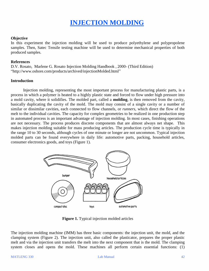
INJECTION MOLDING
Objective
In this experiment the injection molding will be used to produce polyethylene and polypropolene
samples. Then, Satec Tensile testing machine will be used to determine mechanical properties of both
produced samples.
References
D.V. Rosato, Marlene G. Rosato Injection Molding Handbook , 2000- (Third Edition)
“http://www.oshore.com/products/archived/injectionMolded.html”
Introduction
Injection molding, representing the most important process for manufacturing plastic parts, is a
process in which a polymer is heated to a highly plastic state and forced to flow under high pressure into
a mold cavity, where it solidifies. The molded part, called a molding, is then removed from the cavity,
basically duplicating the cavity of the mold. The mold may consist of a single cavity or a number of
similar or dissimilar cavities, each connected to flow channels, or runners, which direct the flow of the
melt to the individual cavities. The capacity for complex geometries to be realized in one production step
in automated process is an important advantage of injection molding. In most cases, finishing operations
are not necessary. The process produces discrete components that are almost always net shape. This
makes injection molding suitable for mass producing articles. The production cycle time is typically in
the range 10 to 30 seconds, although cycles of one minute or longer are not uncommon. Typical injection
molded parts can be found everywhere in daily life: automotive parts, packing, household articles,
consumer electronics goods, and toys (Figure 1).
Figure 1. Typical injection molded articles
The injection molding machine (IMM) has three basic components: the injection unit, the mold, and the
clamping system (Figure 2). The injection unit, also called the plasticator, prepares the proper plastic
melt and via the injection unit transfers the melt into the next component that is the mold. The clamping
system closes and opens the mold. These machines all perform certain essential functions: (1)

MATLENG 330 Lab Manual 43
plasticizing: heating and melting of the plastic in the plasticator, (2) injection: injecting from the
plasticator under pressure a controlled-volume shot of melt into a closed mold, with solidification of the
plastics beginning on the mold's cavity wall, (3) afterfilling: maintaining the injected material under
pressure for a specified time to prevent back flow of melt and to compensate for the decrease in volume
of melt during solidification, (4) cooling: cooling the thermoplastic (TP) molded part in the mold until it
is sufficiently rigid to be ejected, or heating: heating the thermoset (TS) molded part in the mold until it
is sufficiently rigid to be ejected, and (5) molded-part release: opening the mold, ejecting the part, and
closing the mold so it is ready to start the next cycle with a shot of melt.
Figure 2. Injection Molding Machine
IMMs are characterized by their shot capacity. A shot represents the maximum volume of melt that is
injected into the mold. It is usually about 30 to 70% of the actual available volume in the plasticator. The
difference basically relates to the plastic material’s melt behavior, and provides a safety factor to meet
different mold packing conditions. Shot size capacity may be given in terms of the maximum weight that
can be injected into one or more mold cavities, usually quoted in ounces or grams of general purpose
polystyrene (GPPS). Since plastics have different densities, a better way to express shot size is in terms
of the volume of melt that can be injected into a mold at a specific pressure. The rate of injecting the shot
is related to the IMM’s speed and also the process control capability for cycling the melt into the mold
cavity or cavities (fast-slow-fast, slow-fast, etc.).
The injection pressure in the barrel can range from 2,000 to at least 30,000 psi (14 to 205 MPa). The
characteristics of the plastic being processed determine what pressure is required in the mold to obtain
good products. Given a required cavity pressure, the barrel pressure has to be high enough to meet
pressure flow restrictions going from the plasticator into the mold cavity or cavities. The clamping force
on the mold halves required in the IMM also depends on the plastic being processed. A specified
clamping force is required to retain the pressure in the mold cavity or cavities.

MATLENG 330 Lab Manual 44
As it is mentioned above, three basic operations take place in IMM: (1) heating the plastic in the injection
or plasticizing unit so that it will flow under pressure, (2) allowing the plastic melt to solidify in the mold,
and (3) opening the mold to eject the molded product. These three steps are the operations in which the
mechanical and thermal inputs of the injection equipment must be coordinated with the fundamental
properties and behavior of the plastic being processed; different plastics tend to have different melting
characteristics, with some being extremely different. They are also the prime determinants of the
productivity of the process, since the manufacturing speed or cycle time will depend on how fast the
material can be heated, injected, solidified, and ejected. Depending on shot size and/or wall thicknesses,
cycle times range from fractions of a second to many minutes. Other important operations in the injection
process include feeding the IMM, usually gravimetrically through a hopper, and controlling the
plasticator barrel’s thermal profile to ensure high product quality.
Molding Plastics
Most of the literature on injection molding processing refers entirely or primarily to thermoplastic TPs;
very little, if any at all, refers to thermoset TS plastics. At least 90 wt% of all injection-molded plastics
are TPs. Injection molded parts can, however, include combinations of TPs and TSs as well as rigid and
flexible TPs, reinforced plastics, TP and TS elastomers, etc.. During injection molding the TPs reach
maximum temperature during plastication before entering the mold. The TS plastics reach maximum
temperature in the heated molds.
Materials: Polyethylene, Polypropylene
Equipment: Injection Molding Machine (IMM)
Satec Tensile Testing Machine
Caliper
Procedure:
1. Turn on the power button and wait until the screen display shows “2nd initialization completed” 2. Turn the heater switch to clockwise direction and then press the heater button. Before the
temperature control zone reaches the set temperature the warning light will flashing
3. Press the oil heater button. It will make loud noise until the oil temperature reaches 90F ±10
minutes
4. Press the red button (Oil Stop Button) when the loud noise is stop. Turn on the cooling water
supply.
5. Wait until temperature control zone reaches the set temperature.
6. Feed the hopper with Polyethylene compound and Operate Injection Molding Machine (IMM) to
produce 3 standard samples.
7. Replace polyethylene with polypropylene and repeat the procedure.
8. Run the Satec tensile testing machine to determine mechanical properties( yield stress, ultimate
tensile stress, fracture stress, ductility (reduction in area and elongatin%) of samples.

MATLENG 330 Lab Manual 45
DIFFERENTIAL SCANNING CALORIMETRY
Objectives
1. To become familiar with the operation and applications of a Differential Scanning Calorimeter.
2. To identify the type of polymer using its thermal properties from a DSC plot.
References
1. Michael E. Brown, Introduction to thermal analysis: techniques and applications
2. Joseph D. Menczel, R. Bruce Prime, Thermal analysis of polymers: fundamentals and applications
3. David Clifford Bassett, Principles of polymer morphology
Introduction
The Differential Scanning Calorimeter (DSC) determines the temperature and heat flow
associated with material transitions as a function of time and temperature. It also provides quantitative
and qualitative data on endothermic (heat absorption) and exothermic (heat evolution) processes of
materials during physical transitions that are caused by phase changes, melting, oxidation, and other heat-
related changes. This information helps the scientist or engineer identify processing and end-use
performance.
Fig 1a: TA instruments DSC Fig 1b: Schematic diagram of DSC
The DSC instrument works in conjunction with a controller and associated software to make up a
thermal analysis system. A functional DSC system has three major components: the instrument itself,
which contains the system electronics; the cell, which monitors differential heat flow and temperature;
and a cooling accessory. The cooling accessory selected depends on the temperature range desired for
your experiments.
In this experiment you will use a heat flux DSC. This is one in which a sample is heated along
with a reference material with a known specific heat. One of the criteria of this technique is that the
sample and reference material remain at the same temperature during heating. This can be achieved by
setting the machine to heat both the sample and reference material at a specific rate (the rate is set to
20oC/min). This allows the heat flux or difference in energy input between the sample and reference to be
measured.
Maintaining a constant supply of heat to both materials would not maintain a minimal
temperature difference between them. Instead, a computer is connected to the machine, and using the
software and various signals from the calorimeter, it “decides” when to supply heat to either material.

MATLENG 330 Lab Manual 46
This information is then dealt with by the computer software and presented in the form of a graph of the
energy changes versus the temperature. A standard DSC curve for a polymer is shown in fig. 2.
Fig 2: Standard DSC output for a polymer
From the graph, it can be seen that a sudden upward jump in the curve signifies an exothermic
process. A sudden drop in heat flux indicates an endothermic process.
In case of polymers, the technique takes advantage of the energy changes involved in the various
phase transitions of certain polymer molecules. This allows several properties of the material to be
ascertained; like glass transitions, "cold" crystallization, phase changes, melting, crystallization, product
stability, cure/cure kinetics, oxidative stability and degradation temperatures.
Polymer Morphology
Small molecules usually have crystalline solids, which are highly-ordered 3-dimensional arrays of
the molecules. Solid polymers can be crystalline or amorphous (disordered arrangements of randomly
coiled and entangled chains). Thermoplastics usually are semi crystalline - a combination of crystalline
and amorphous regions. The properties of thermoplastics are strongly influenced by their morphology.
Highly crystalline polymers are rigid, high melting, and less affected by solvent penetration.
Crystallinity makes polymers strong, but also lowers their impact resistance.
Polymer chains with branches or irregular pendant groups cannot pack together regularly enough
to form crystals. These polymers are said to be amorphous. They are softer, have lower melting points,
and are penetrated more by solvents than are their crystalline counterparts.
Semi-crystalline polymers have both crystalline and amorphous regions. Semi-crystallinity is a
desirable property for most plastics because they combine the strength of crystalline polymers with the
flexibility of amorphous. Semi-crystalline polymers can be tough with an ability to bend without
breaking. The crystals are small and connected to the amorphous regions by polymer chains so there may
be no sharp well-defined boundaries between the two types of regions.
Fig 3: Lamellar structure of semi-crystalline polymer

MATLENG 330 Lab Manual 47
Glass transition temperature (Tg)
In the study of polymers and their applications, it is important to understand the concept of the
glass transition temperature, Tg. As the temperature of a polymer drops below Tg, it behaves in an
increasingly brittle manner. As the temperature rises above the Tg, the polymer becomes more rubber-
like. This is predominantly observed in amorphous polymers. On heating, an amorphous polymer, it
changes from being hard, brittle and glass like to being a soft rubber like substance. As the polymer is
cooled, molecules have less freedom and become bonded to each other. As the percentage of bonded
molecules increases, there comes a point at which long-range connectivity occurs and the polymer reverts
to a glass like phase again.
This point may be identified as a dip on a graph of heat flux versus increasing temperature, this is
due to the molecule having a greater degree of freedom and absorbing energy to maintain the same rate
of heating as the reference. It can then be concluded that glass transition is an endothermic process.
Unlike a transition from a solid to a liquid, or liquid to gas, the energy change involved in glass transition
(a second order phase change) is quite small. Fully crystalline polymers have no glass transition and their
structure remains intact until the melting point. The glass transition temperature is between 0.5 and 0.8 of
the melting temperature. The table below lists the factors affecting Tg of polymers:
Lower Tg is due to Higher Tg is due to
Main chain flexibility Main chain rigidity
Flexible side chains Bulky or rigid side chains
Increase in Tacticity Increased cohesive energy
density
Increased symmetry Increased molecular weight
Branching Increased polarity
Addition of plasticizers or
diluents Cross linking
Temperature of crystallisation (Tc)
Continuing to heat a polymer past its Glass transition temperature eventually leads to another
transition. Before this point in the thermal analysis, the molecules are arranged in a random fashion and
are coiled around each other in an unfavourable manner. A transition occurs when molecules acquire
enough freedom to move into a more energetically stable phase, i.e. a crystalline state. This would
indicate that the phase following the glass transition is metastable and when sufficient energy is supplied,
its molecules adapt a more stable (lower energy) arrangement. Because the molecules in a crystalline
solid have less freedom than those in a flexible rubbery one, the transition between these two states is
exothermic and may be seen as a brief upward “jump” in the graph.
Temperature of melting (Tm)
This is the point at which the (now crystalline) polymer molecules have gained enough
vibrational freedom to break free from the solid binding forces and form a liquid. Due to the increased
freedom of these molecules, the DSC graph should take a sudden dip at this temperature to indicate the
endothermic nature of the process, which is a first order transition. The melting point of any substance
can be given by:

MATLENG 330 Lab Manual 48
m
mm
S
HT
ΔHm is the enthalpy of melting and ΔSm is the change of entropy involved in the melting phase (entropy
of fusion).
The Flory equation (1), well known to the polymer chemist but rarely used by the thermal analyst,
provides a tool to calculate polymer crystal molecular weight and molecular weight distribution from
DSC melting curves. The relationship between polymer molecular weight (MW, in g mol-1) and the
melting temperature (T, in K) is given by:
MW = [2*R*T*Tmax] / [H (Tmax -T)]
Where R is the molar gas constant (8.314 Jg-1mol-1), H is the enthalpy of fusion for 100% crystalline
material (in Jg-1), and Tmax is the maximum melting temperature of the polymer archetype (in K).
Degradation Temperature (TD)
The final transition on a DSC graph is the degradation temperature, TD. At this point in the
heating cycle, individual bonds between atoms start to break as the vibrations become more and more
fierce until eventually; individual polymer molecules decompose into their components. Depending on
the nature of the substance under investigation, this process can be either endothermic or exothermic.
Materials: Four unknown polymer samples, Nitrogen atmosphere, with a gas flow rate of 50 ml/min
Equipments: TA instruments DSC Q 2000, tweezers, sample pans and lids, gloves
Procedure
* Follow the instructions given by your TA carefully; care should be taken while preparing samples
to avoid contamination.
** DO NOT TRY TO OPEN OR CLOSE THE LID OF THE SAMPLE HOLDER MANUALLY **
1. Precisely measure 5-10 mg of the sample marked for your section.
2. Place the sample in the sample pan and cover with the lid and record the weight in milligrams. This
will be the sample size to be entered on the system.
3. Using the Q2000 software, go to stand by temperature. Then click ‘lid open’ and wait for the lid of
the sample holding chamber to be opened. Place the sample pan and close the lid by selecting the ‘lid
close’ prompt on the system.
4. Select the procedure (specifying the ramp heating speed and temperature range) marked for your
section.
5. Enter the weight of the sample in the ‘sample size’ section.
6. Select the specified path in the C drive to save the test results.
7. Click ‘Event on’ and click the ‘green play icon’ to start the test.

MATLENG 330 Lab Manual 49
8. Once the test is completed, click ‘Event off’ and press the ‘red stop icon’ to stop the test.
9. Launch the TA analysis software and open the file containing your test results (DSC plot).
10. Your TA will show you how to apply the limits on the plot to determine the Tg, Tm and Tc of the
sample.
Results
* Each section will test one polymer sample and the data from all the sections will be compiled and
uploaded on D2L or mailed to the students for analysis.
1. Tabulate the Tg, Tm and Tc of each sample from the plots.
2. Identify the polymer based on the thermal properties collected and cite suitable references.
3. Copy and paste the DSC plots for each material and label the material along with its thermal
properties.

MATLENG 330 Lab Manual 50
APPENDIX A
STRESS CORROSION CRACKING BEHAVIOR OF ALLOY 690 IN HIGH TEMPERATURE
HYDROGEN SUPERSATURATED STEAM
ABSTRACT
Intergranular stress corrosion cracking (IGSCC) of an Inconel alloy 690 was investigated by exposing it
to 300-400oC in deaerated hydrogen supersaturated steam. The alloys were tested in the as-received
condition. Crack growth rates were measured in-situ for the above alloy using modified wedge-opening-
load (M-WOL) linear elastic fracture specimens under constant displacement conditions. The applied
stress intensity factors (KI) used varied from 29-90 MPam1/2. Activation energy of 120 kJ/mol was found
for crack growth rates as a function of temperature. This activation energy is close to the one
corresponding to gb self-diffusion of nickel. In addition, it was found that the apparent crack growth
rates (da/dt) exhibited a linear dependence with KI given by da/dt = AKI. Microstructurally, crack
propagation in this alloy was predominant along the grain boundaries. It is suggested that high fugacity
hydrogen was generated at the tip of the crack as a result of reaction of H2O with Cr in a freshly exposed
fracture surface leads to IGSCC.
INTRODUCTION
Extensive work worldwide has been devoted to disclosing the mechanisms involved during the
intergranular stress corrosion cracking (IGSCC) of pressurized water reactors (PWR) made of Inconel
alloys1-3. From these works, it is well known that Inconel alloy 600 is susceptible to SCC under
hydrogen supersaturated steam at temperatures above 300oC. The objective of the experiments
described in this paper is to determine the mechanisms involved in the IGSCC.
THEORETICAL BACKGROUND
The mechanistic aspects involved in the SCC of Inconel alloys are far from being resolved 4-7. In
general, it has been found that heat treating can lead to Cr depletion of the grain boundaries (gbs) in
precipitation hardened Ni-base alloys as a result of gb chromium carbide precipitation3, (condition known
as sensitized in other alloy systems). This condition should be highly susceptible to SCC, in contrast
with the experimental reports4. Yet, these alloys become increasingly susceptible in the milled annealed
condition1,4.
Moreover, it has been found that crack propagation occurs preferentially along gbs4-7. In addition, grain
boundary segregation which can reduce the cohesive strength of the grained structure is not able to
account for the IGSCC susceptibility for the present amounts of segregated impurities3. The role of
hydrogen is not clear either. It has been found that dissolved hydrogen in high temperature steam
enhances the IGSCC susceptibility in inconel alloys at 300-360oC in pure water2. In particular, it has
been found that as the dissolved hydrogen concentration is increased, the time for cracking in PWR’s
decreases dramatically2. Yet the mechanisms proposed are not able to account for all the experimental
facts.
Alternatively, when alloy 690 has been employed to replace alloy 600, the SCC susceptibility is
significantly reduced under the PWR environments8. Apparently, increasing the Cr content from 15 %
(alloy 600) to 30% (alloy 690) leads to improved cracking resistance. Although, there is not a clear
explanation for this behavior, it seems that the alloy repasivation kinetics is enhanced at increasing Cr
contents8. Electrochemical studies3, on the effect of hydrogen on the SCC susceptibility of alloys 600 and
690 indicate that the IGSCC is cathodic in nature, despite the lack of evidence for hydrogen having a
detrimental effect on the passive film properties of these alloys3.
In addition, the activation energies associated with IGSCC in inconel alloys have been reported to be of
the order of 74-138 kJ/mol4, which suggest Ni gb self-diffusion as the rate limiting mechanism.
Moreover, the reported activation energies seem to be inversely related to the applied stress intensity
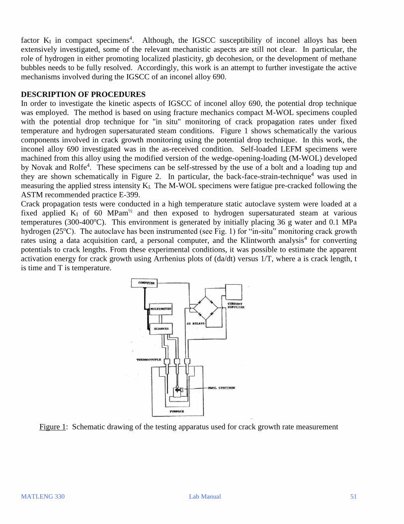
MATLENG 330 Lab Manual 51
factor KI in compact specimens4. Although, the IGSCC susceptibility of inconel alloys has been
extensively investigated, some of the relevant mechanistic aspects are still not clear. In particular, the
role of hydrogen in either promoting localized plasticity, gb decohesion, or the development of methane
bubbles needs to be fully resolved. Accordingly, this work is an attempt to further investigate the active
mechanisms involved during the IGSCC of an inconel alloy 690.
DESCRIPTION OF PROCEDURES
In order to investigate the kinetic aspects of IGSCC of inconel alloy 690, the potential drop technique
was employed. The method is based on using fracture mechanics compact M-WOL specimens coupled
with the potential drop technique for "in situ" monitoring of crack propagation rates under fixed
temperature and hydrogen supersaturated steam conditions. Figure 1 shows schematically the various
components involved in crack growth monitoring using the potential drop technique. In this work, the
inconel alloy 690 investigated was in the as-received condition. Self-loaded LEFM specimens were
machined from this alloy using the modified version of the wedge-opening-loading (M-WOL) developed
by Novak and Rolfe4. These specimens can be self-stressed by the use of a bolt and a loading tup and
they are shown schematically in Figure 2. In particular, the back-face-strain-technique4 was used in
measuring the applied stress intensity KI. The M-WOL specimens were fatigue pre-cracked following the
ASTM recommended practice E-399.
Crack propagation tests were conducted in a high temperature static autoclave system were loaded at a
fixed applied KI of 60 MPam½ and then exposed to hydrogen supersaturated steam at various
temperatures (300-400oC). This environment is generated by initially placing 36 g water and 0.1 MPa
hydrogen (25oC). The autoclave has been instrumented (see Fig. 1) for “in-situ” monitoring crack growth
rates using a data acquisition card, a personal computer, and the Klintworth analysis4 for converting
potentials to crack lengths. From these experimental conditions, it was possible to estimate the apparent
activation energy for crack growth using Arrhenius plots of (da/dt) versus 1/T, where a is crack length, t
is time and T is temperature.
Figure 1: Schematic drawing of the testing apparatus used for crack growth rate measurement

MATLENG 330 Lab Manual 52
Figure 2: Schematic representation of the modified WOL specimen load assembly
The effect of applied KI on the rate of crack growth was also estimated in the as-received alloy by
exposing the M-WOL specimens to the SCC environment. These specimens were previously loaded at
applied KI values in the range of 29-90 MPam½and then exposed to hydrogen supersaturated steam at
370oC. The as-received microstructure and type of carbides was evaluated by optical and scanning
(SEM), electron microscopy. Also, crack paths and crack lengths, were characterized by these means.
RESULTS AND DISCUSSION
In the as-received Inconel alloy 690, the exhibited microstructure consisted of stacking faults and fine
carbides, both within and along grain boundaries (Fig. 3a). Also, the path followed by these specimens
was predominantly intergranular with some branching as shown in Figs 3a-b.
(a)
(b)
Figure 3: Crack paths exhibited in Inconel 690. (a, b) Notice the presence of grain boundary carbides, as
well as significant stacking faults within the bulk, including some degree of crack branching.
Exposure of M-WOL specimens to hydrogen supersaturated steam enabled the determination of an
apparent activation energy for crack growth (da/dt) in specimens loaded at 60 MPam1/2. The
experimentally determined activation energy was of the order of 120 kJ/mol as shown in Fig. 4. which is
in good agreement with the activation energy reported for grain boundary self-diffusion of Ni which is

MATLENG 330 Lab Manual 53
115 kJ/mol4. The effect of the applied KI on (da/dt) was also evaluated as shown in Fig. 5. Notice from
this log-log graph a linear trend for crack growth with the applied KI suggesting that there is a stable
stage II for crack growth. Accordingly, crack growth can be described by an empirical expression of the
type da/dt = AKIn where n = 1.
Mechanistically speaking, because of the cathodic nature of IGSCC crack propagation, this work will
make emphasis on the possible role of hydrogen. From the work of Shewmon et coworkers4, alloy
passivation can be described by
2/3Cr + H2O = 1/3 Cr2O3 + H2 (1)
As a result of this reaction, it is likely to release hydrogen at the crack tip with extremely high fugacities.
Increasing the Cr levels from 15 to 30 % will not diminish this effect. Enough hydrogen release will be
available in the crack tip regions as fresh metal is exposed to H2O.
1.00E-10
1.00E-09
0.00145 0.0015 0.00155 0.0016 0.00165 0.0017
1/T (K-1)
da/d
t (m
/s)
Figure 4: Arrhenius plot of da/dt versus 1/T for as-received alloy 690 M-WOL specimens exposed to
hydrogen supersaturated steam under an applied KI of 60 MPam1/2.
1E-14
1E-13
1E-12
1000 10000 100000
KI (MPam1/2
)
da/d
t (m
/s)
Figure 5: da/dt versus applied KI for as-received alloy 690 M-WOL specimens exposed to hydrogen
supersaturated steam at 370oC.

MATLENG 330 Lab Manual 54
Evidence for this effect has been experimentally shown by Ulla Ehrnsten et al8. In their work, they found
that when excess hydrogen was removed in an inconel alloy exposed to hydrogen overpressure, the
electric resistance of the inconel surface as well as the potential drop signal, both increased significantly,
indicating that the alloy was able to repassivate according to reaction (1). Hence, high hydrogen
fugacities product of reaction 1 developed at the tip of the crack which in turn promoted IGSCC. In the
300-400oC range, hydrogen preferentially diffuses along the grain boundaries where it can react with
segregated carbon to locally produce methane bubbles as described by Shewmon et al4. In the present
work, a fine distribution of carbides was found along gbs as shown in Fig. 3a. Hence, it is expected that
gb segregated carbon will be reduced to levels where methane formation might be minimal. Yet,
alternative hydrogen effects might be active such as those suggested by Saario et al9 in their model on the
selective dissolution vacancy creep, or through hydrogen induced gb plasticity5-9, both of which can
account for IGSCC.
Finally, the rate of crack propagation dependance with the applied KI indicates that stage II crack
propagation follows an apparent linear trend with the applied stress intensity factor. However, when
branching occurs, crack propagation should be independent of the applied KI and crack length during
stage II4. Since the degree of branching is minimal, under the SCC conditions employed, crack growth
might exhibit a linear trend with the applied KI to account for the experimental outcome, but further
analysis is needed to resolve this issue.
SUMMARY
M-WOL specimens of alloy 690 were exposed at 300-400oC in deaerated hydrogen supersaturated steam
under an applied stress intensity factor (KI) of 60 MPam1/2. It was found that the alloy exhibited
intergranular stress corrosion cracking in the as received condition. An activation energy of 120 kJ/mol
was found which is close to the one reported for gb selfdifusion of nickel. In addition, a linear
dependance for the rate of crack propagation was found as a function of the aplied stress intensity factor,
which can be described by da/dt = AKIn and n equal to 1. The corrosive environment was predominantly
cathodic in nature. Hence, the mode of IGSCC is expected to be dominated by the development of high
fugacity hydrogen at the tip of the crack as fresh surfaces come into contact with the steam.
REFERENCES
1. Environmental Degradation of Materials in Nuclear Power Systems-Water Reactors, Proceedings
Third Intl. Symp. Traverse City Michigan, TMS, 1988.
2. D. Noel, O. De Bouvier, F. Foct, T. Magnin, J-D. Mithieux, and f. Vaillant, Int. Conf. on
Corrosion-Deformation Interactions, Eurocorr’96, Nice France, Sept. 24-26, 1996.
3. I. Lenartova, M. Habashi, V. Vodarek, J. Galland, M. Tvrdy, and L. Hyspecka, Int. Conf. on
Corrosion-Deformation Interactions, Eurocorr’96, Nice France, Sept. 24-26, 1996
4. C. H. Shen and P. G. Shewmon, Metall. Trans. A, , 21A, 1261, (1990).
5. F. Foct, O. deBouvier, T. Magnin, and D. Noel, Int. Conf. on Corrosion-Deformation
Interactions, Eurocorr’96, Nice France, Sept. 24-26, 1996
6. C. Newman and M. Saito, Corrosion-deformation interactions, CDI-9, Conf . Proc.,
Fontainebleau-France, Oct. 5-7, 1992., Les editions de physique.
7. G. Bond, I. M. Robertson,and H. K. Birnbaum, Acta Metall, 36, 2193 (1988).
8. U. Ehrnesten, J. Lagerstrom, T. Saario, , and H. Hanninen, Int. Conf. on Corrosion-Deformation
Interactions, Eurocorr’96, Nice France, Sept. 24-26, 1996
9. T. Saario, P. Aaltonen, , page 841, 7th Symposium on Env. Degradation of Materials in Nuclear
Power Systems-Water Reactors, 1995.