DOING PHYSICS WITH MATLAB

THE FINITE DIFFERENCE METHOD FOR THE NUMERICAL

ANALYSIS OF SERIES RCL CIRCUITS

MATLAB DOWNLOAD DIRECTORY

CNsRCL.m

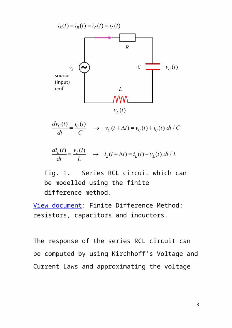
Computation of voltages, current, and energies for series RCL

circuits using the finite difference method. The Matlab function

findpeaks is used to estimate frequencies (periods) and phases.

An interesting circuit is obtained by connecting a resistor,

capacitor and inductor in series with a source (input) emf

(figure 1). The behaviour of the circuit is like an object at the end

of a spring - it oscillates. There is a continual exchange of energy

between the energy source and the energies stored in the

capacitor and inductor. In a mechanical system, an object

oscillates back and forth around an equilibrium position. In the

electrical circuit, it is the charge that oscillates. The oscillating

charge produces an alternating current and alternating voltage

drops across the resistor, capacitor and inductor. The frequency

of the oscillation depends only upon the values of the

1

capacitance C and inductance L. This natural frequency f0

(resonance frequency) is given by

(1)

The response of the series RCL circuit is that of a damped

harmonic oscillator. The damping being dependent upon the

resistance R. The greater the value of the resistance, the greater

the damping effect.

Fig. 1. Series RCL circuit which can be modelled using the finite difference method.

2

View document: Finite Difference Method: resistors, capacitors and inductors.

The response of the series RCL circuit can be computed by using

Kirchhoff’s Voltage and Current Laws and approximating the

voltage across the capacitor and current through the inductor

using the finite difference method.

The script CNsRCL.m is used to model the series RCL circuit. In

the script, the first letter of a variable that is a function of time or

a complex variable is a lowercase letter. A variable that start with

an uppercase letter is independent of time or a real quantity. For

example, vS is the variable for the input emf and is calculated at

each time step, whereas the variable VS is the peak value of the

source emf.

A step function (OFF/ON) or a complex sinusoidal function can

be selected as the source emf using the variable flagV (flagV = 1

for a step function or flagV = 2 for a sinusoidal function). The

source emf can be changed within the switch/case script. The

time scales for a simulation are also set within the switch/case

script.

3

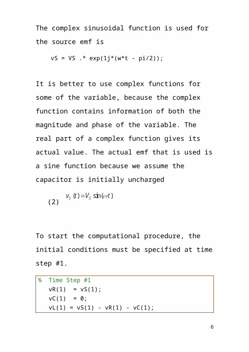
The complex sinusoidal function is used for the source emf is

vS = VS .* exp(1j*(w*t - pi/2));

It is better to use complex functions for some of the variable,

because the complex function contains information of both the

magnitude and phase of the variable. The real part of a complex

function gives its actual value. The actual emf that is used is a

sine function because we assume the capacitor is initially

uncharged

(2)

To start the computational procedure, the initial conditions must

be specified at time step #1.

% Time Step #1 vR(1) = vS(1); vC(1) = 0; vL(1) = vS(1) - vR(1) - vC(1); iS(1) = vR(1) / R; iS(1) = iS(1) + vL(1) * dt / L; vC(1) = vC(1) + iS(1) * dt / C; vR(1) = iS(1) * R; vL(1) = vS(1) - vR(1) - vC(1);

4

The values of the voltage and current parameters are calculated

by implementing the finite difference method. Note: the voltage

across the capacitor uses an average value of the current over

two time steps to improve the accuracy of the numerical

approximation (half-step method).

% Time Steps #2 to #N for c = 2 : N iS(c) = iS(c-1) + vL(c-1) * dt/L; vR(c) = iS(c) * R; vC(c) = vC(c-1) + 0.5*(iS(c)+iS(c-1)) * dt / C; vL(c) = vS(c) - vR(c) - vC(c); end

For accurate results, the time interval dt should be chosen so

that it is much smaller the period of the natural oscillation

(3)

% Resonance Frequency f0, period T, time step dt f0 = 1/(2*pi*sqrt(L*C)); T0 = 1/f0; dt = T0 /1000;

5

From the values of R, C and L, the impedances Z of the circuit

elements for the sinusoidal source emf are calculated as shown

in the Table.

% Impedance calculations XC = 1/(w*C); ZC = -1j*XC; XL = w*L; ZL = 1j*XL; ZR = R; Z = ZR + ZC + ZL;

Energy is dissipated by a current through the resistor and energy

is stored in the electric field of the capacitor plates, and stored in

the magnetic field surrounding the coil of the inductor. The

power and energy as functions of time t can easily be

computed.

% Powers and energy pS = real(vS) .* real(iS); pR = real(vR) .* real(iS); pC = real(vC) .* real(iS); pL = real(vL) .* real(iS); uS = zeros(1,N); uR = zeros(1,N); uC = zeros(1,N); uL = zeros(1,N); for c = 2 : N uS(c) = uS(c-1) + pS(c)*dt; uR(c) = uR(c-1) + pR(c)*dt; uC(c) = uC(c-1) + pC(c)*dt; uL(c) = uL(c-1) + pL(c)*dt; end

6

Our series RCL circuit is complicated. We can not simply add the

voltages across the resistor, capacitor and inductor because of

the phase differences between these voltages. However, in the

modelling, we use a complex exponential function to simulate a

real sine function source voltage. The computed values for the

circuit current and voltages are all computed as complex

functions. So, these complex functions contain information of

the magnitudes and phases. The script below shows the

calculation of the phases at a time step given by the variable nP.

By changing the value of nP, you can see the phases at different

times.

% Phases voltage: phi and current theta at time step nP [degrees] nP = N-500; phiS = rad2deg(angle(vS(nP))); phiR = rad2deg(angle(vR(nP))); phiC = rad2deg(angle(vC(nP))); phiL = rad2deg(angle(vL(nP))); thetaS = rad2deg(angle(iS(nP))); phiSR = phiS - phiR;

7

The response of the circuit may result in oscillations. The period

TPeaks of the oscillation can be approximated by finding the time

intervals between peaks using the Matlab function findpeaks as

shown in the code in the Table.

% Find peaks in vS and corresponding times% Calculate period of oscillations% May need to change number of peaks for estimate of period: nPeaks [iS_Peaks, t_Peaks] = findpeaks(real(iS)); nPeaks = 3; T_Peaks = (t(t_Peaks(end))- t(t_Peaks(end-nPeaks)))/(nPeaks); f_Peaks = 1 / T_Peaks;

If no peaks are found, you may get an error message. If this

happens, simply set the statements to comments using % and set

f_Peaks = 0 and T_peaks = 0.

A summary of the input and calculated parameters is displayed

in the Command Window. The results of the modelling are

displayed graphically in a series of plots as shown in the

following simulations.

8

RESPONSE TO A STEP FUNCTION OFF / ON

The response of the RCL circuit is like that of a mass at the end of

a string.

Natural frequency for the series RCL is

(1)

Natural frequency of oscillation of mass / spring system is

In this analogy

where b is the damping coefficient of the velocity term in the equation of motion of the mass on a spring.

When an object attached to a spring is disturbed, is motion can

often be classified as underdamped, critically damped or

overdamped. Critical damping provides the quickest approach to

zero amplitude for a damped oscillator. With less damping

(underdamping) it reaches the zero position more quickly, but

oscillates around it. With more damping (overdamping), the

9

approach to zero is slower. For our series RCL circuit, the

damping is determined by the value of the resistance.

The critical damping resistance is given by

When the system is underdamped and when

the system is overdamped.

When there is underdamping , the system vibrates

at its natural frequency until the oscillations die away. Any

sudden changes in the source emf may produce a ringing effect,

where the current oscillates at the resonant (natural) frequency

determined by the values of C and L as given by equation 1. The

amplitude of the current dies away exponentially.

10

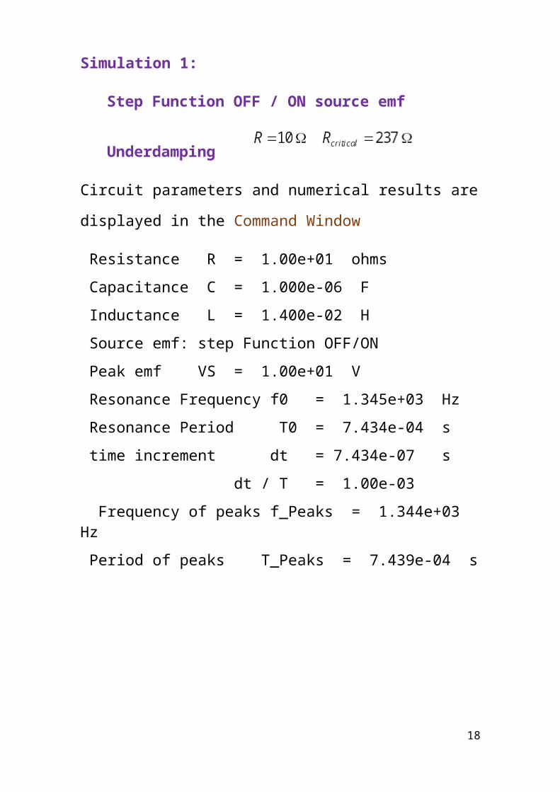
Simulation 1:

Step Function OFF / ON source emf

Underdamping

Circuit parameters and numerical results are displayed in the

Command Window

Resistance R = 1.00e+01 ohms

Capacitance C = 1.000e-06 F

Inductance L = 1.400e-02 H

Source emf: step Function OFF/ON

Peak emf VS = 1.00e+01 V

Resonance Frequency f0 = 1.345e+03 Hz

Resonance Period T0 = 7.434e-04 s

time increment dt = 7.434e-07 s

dt / T = 1.00e-03

Frequency of peaks f_Peaks = 1.344e+03 Hz

Period of peaks T_Peaks = 7.439e-04 s

11

Figure 2 shows the plots of the current as a function of time for

two underdamped systems. When the resistance R is increased

from R = 10 Ω to R = 40 Ω, the oscillations die away more quickly

due to the increase in damping. Figure 3 shows the voltages

across the resistor, capacitor and inductor.

The natural frequency of the oscillation calculated from

equation 1 is

The value of the natural frequency from the model using

the findpeaks function is

So, we have excellent agreement between the two values.

12

Fig.2. The ringing effect of the step function source emf. The oscillations die way exponentially. The larger the resistance R, the more rapidly the oscillations decrease.

13

Fig. 3. The voltages as function of time. The ringing effect is very noticeable from the plots. The blue curves represents the source emf.

14

We can see clearly from figure 3 that there is a rad phase

difference between for the voltage across the capacitor and the

voltage across the inductor (a peak in vC corresponds to a trough

in vL). Through careful examination of figure 3, we can state that

Hence, we can conclude, The voltage across the capacitor lags

the voltage across the resistor by rad; the voltage across

the inductor leads the voltage across the resistor by rad;

and the voltage across the inductor leads the voltage across the

capacitor by rad.

We can also get the phase values from the Command Window

using the findpeaks command. The findpeaks command is used

to find the indies for the times of the least peak in the voltages.

[a b] = findpeaks(real(vR)) →

a = 0.7942 0.6149 0.4761 0.3686 0.2854

b = 782 1782 2783 3784 4784

The times for the last peaks are

resistor t(4784) = 3.5559 ms

capacitor t(5041) = 3.7469 ms

15

inductor t(4527) = 3.3648 ms

We can calculate the period from the values of b given from the

findpeaks function

period T = ( t(4784) -t(1782) ) /3 (time between 3 peaks)

T = 0.7439 ms

We can now find the phases by comparing the time difference

between peaks and the period and expressing the phase angle in

degrees.

Phase difference between vC and vR

Phase difference between vL and vR

Phase difference between vL and vC

16

17

Figures 4 and 5 shows the exchanges of energy occurring in the

circuit as functions of time. The emf source provides energy to

the circuit. When a current passes through the resistance, energy

is absorbed and dissipated as thermal energy resulting in an

increase in temperature of the resistor. The capacitor stores

energy as it charges and supplies energy to the circuit as it

discharges. For our step function emf input voltage, after the

oscillations die away, the capacitor becomes fully charged and

stores energy since the capacitor acts like an open circuit, the

current falls to zero. The inductor stores in the magnetic

surrounding the coil energy as the current through it increases.

When the current finally drops to zero, the inductor no longer

stores or supplies energy to the circuit. For the power curves as

functions of time, when the power is positive, energy is either

dissipated or stored. When the power is negative, the stored

energy is returned to the circuit.

18

Fig. 4. The power absorbed or supplied by the circuit elements. The blue curves represent the source emf.

19

Fig. 5. The energy exchanges in the circuit.

20

The power is the rate of energy transfer

(4)

If you “mentally” differentiate an energy plot w.r.t. time you get

the power plot as a function of time. For example, in figure 5, the

first peak in the energy plot for the capacitor occurs at the time

t = 0.74149 ms. At this time, the power pC is zero.

It is very easy to change any of the parameters in the script, and

see immediately, how the response of the circuit changes. For

example, figure 6 shows the response when the capacitor value

is decreased by a factor of 9. The natural frequency is now

4035 Hz.

21

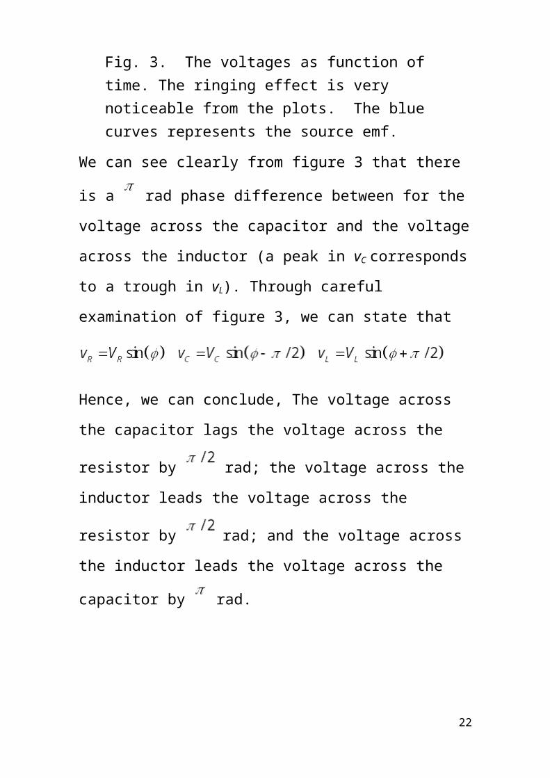
Fig. 6. A decrease in capacitance C results in higher frequency oscillations.

22

Simulation 2:

Step Function OFF / ON source emf

Underdamping / Critical damping / overdamping

The following figures shows the changes in the damping of the

voltages as the resistance of the circuit is increased.

23

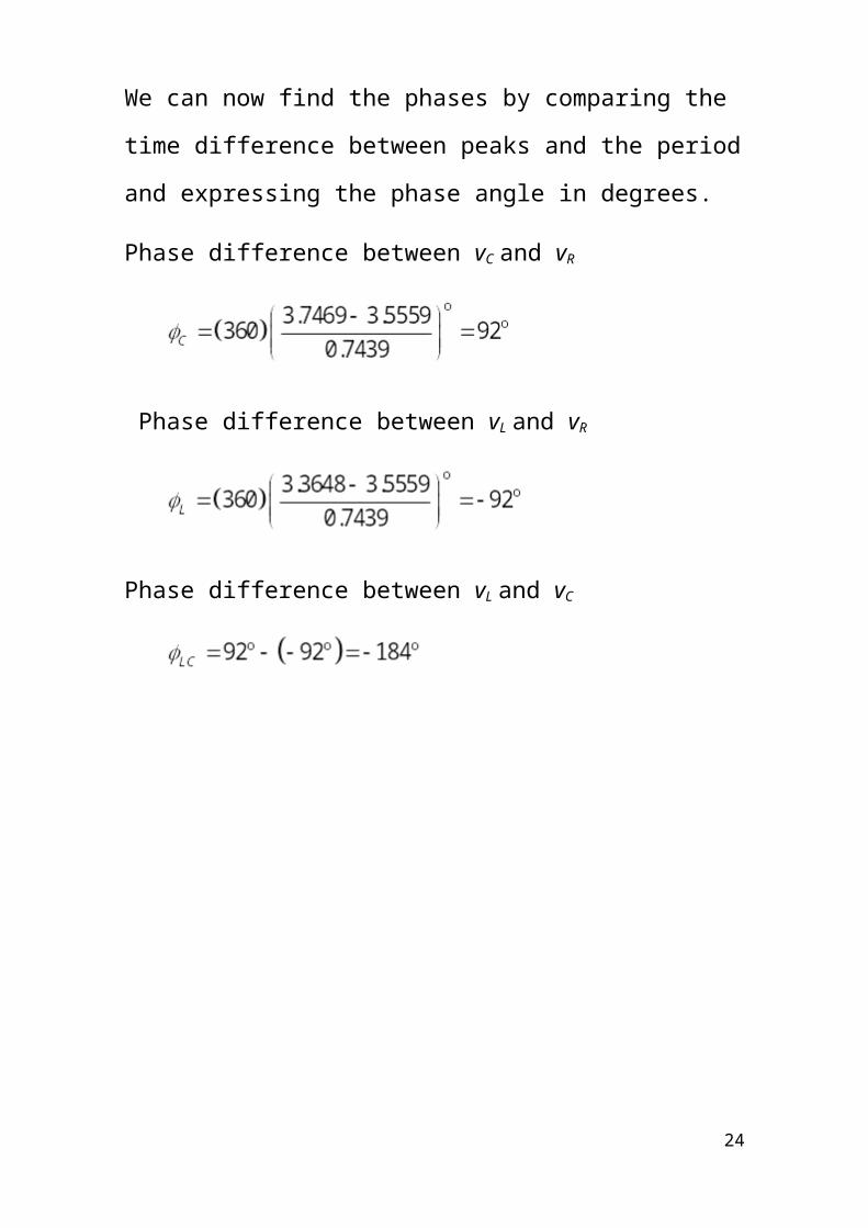
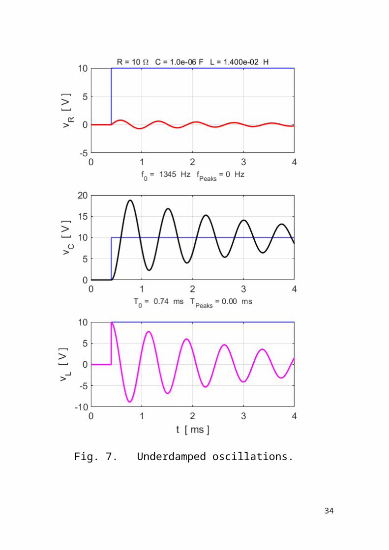
Fig. 7. Underdamped oscillations.

24

Fig. 8. Heavily underdamped damped oscillations.

25

Fig. 10. Critically damped signals – no oscillations. In the script need to comment the lines for findpeaks.

26

Fig. 10. Overdamped signals – no oscillations. In the script need to comment the lines for findpeaks.

27

RESPONSE TO A SINUSOIDAL SOURCE VOLTAGE

A mechanical oscillator will vibrate at the driving frequency. As

the driving frequency approaches the natural frequency of

vibration of the system, the amplitude of the oscillation can be

become very large. This phenomenon is called resonance.

Resonance occurs in a series RCL circuit. The current in the circuit

oscillates at the same frequency as the sinusoidal source emf.

When the source emf frequency matches the natural frequency

as given by equation 1, the amplitude of the oscillation is a

maximum for a given amplitude of the source emf.

Simulation 3: Sinusoidal source emf

Figure 11 shows two plots, one where the source frequency is

equal to the natural frequency and the

second plot, the source frequency higher than the natural

frequency .

Warning: It always takes a few cycles before the current (or

voltages) to vary sinusoidally with a constant amplitude (peak

value). The amplitudes of the sinusoidal current oscillations are:

28

At resonance the total circuit impedance is equal to the

resistance. The effects of the capacitor and inductor cancel each

other. So, the current in the circuit is

29

Fig. 11. The current in the circuit is a maximum when driven at the resonance frequency.

Figures 12 shows the voltage plots when the frequency of the

complex exponential function is equal to the natural frequency

. After a few cycles, the effects of the

capacitor and inductor cancel. The magnitudes of the voltage

across the capacitor is equal to the magnitudes of the voltages

across the inductor but they are rad (180o) out of phase

. So, the voltage across the resistor is identical

to the source emf .

It is better to use a complex exponential function rather than the

sine function for the source emf as we can extract both the

magnitude and phase from it. This means that we can compare

the phases across the resistor, capacitor, inductor and current

with the phase of the source emf. Figure 9 shows the phasor

diagram when for the voltages at one instant

when t = 9.50 ms and at a slightly later time t = 9.70 ms. The

voltage of the source emf is in phase with voltage across the

resistor at resonance.

30

31

Fig. 12. The voltages as a function of time when the source frequency is equal to the natural frequency.

32

Fig. 13. Phasor diagram for the voltages at times t = 9.50 ms and time t = 9.70 ms. Each phasor rotates

anticlockwise with angular velocity .

33

Remember, you cannot add ac voltages as simple numbers, they

must be added like vector quantities. We can verify this in the

Command Window by displaying the voltage and current values.

You can compare the numerical results in the Table with the

phasors in figure 13.

t(9700) = 0.0097

vS(9700) = -9.4910 + 3.1499i

vR(9700) = -9.6073 + 3.1895i

vC(9700) = 12.6747 +38.2413i

vL(9700) = -12.5583 -38.2810i

vR(9700)+vC(9700)+vL(9700) =-9.4910 + 3.1499i

iS(9700) = -0.2402 + 0.0797i

rad2deg(angle(vS(9700))) = 161.6400

rad2deg(angle(vR(9700))) = 161.6343

rad2deg(angle(vC(9700))) = 71.6628

rad2deg(angle(vL(9700))) = -108.1624

rad2deg(angle(vL(9700))) = 161.6343

rad2deg(angle(iR(9700))) = 161.6343

34

The circuit impedances are calculated within the script and

displayed in the Command Window.

Sinusoidal Source emf

Source frequency fS = 1.00e+03 Hz

Impedance: resistance ZR = 4.00e+01 ohms

Impedance: capacitance ZC = 0.000e+00 -1.592e+02 ohms

capacitance phase angle phiC = -90.0 deg

Impedance: inductance ZL = 0.000e+00 1.592e+02 ohms

inductance phase angle phiL = 90.0 deg

Impedance: total Z = 4.00e+01 -2.81e-12 ohms

Impedance: magnitude |Z| = 4.00e+01 ohms

impedance phase angle phiZ = -0.00 deg

The impedance of the capacitor is equal in magnitude of the

impedance of the inductor and 180o out of phase at the

resonance frequency. So, the total impedance is equal to the

resistance value and the phase of the circuit impedance is zero.

The impedances given in the above Table were calculated from

the equations

(5)

35

The impedance is defined as the ratio of the voltage to the

current.

(6) Z is independent of time

We can calculate the values of the impedances in the Command

Window using equation 6 at any time step and compare the

values with the values given from relationships given in

equation 5.

t(9700) = 0.0097

ZR abs(vR(9700)/iS(9700) = 40.0000

ZC abs(vC(end)/iS(end)) = 159.1907

ZL abs(vL(end)/iS(end)) = 159.1956

Z abs(vS(end)/iS(end)) = 39.5141

Figure 14 shows the phase plots (I vs V plot). The phase plot for

the resistor is a straight line. The straight line indicates that the

voltage and current for the resistor are in phase. The reciprocal

of the slope of the line is equal to the value of the resistance.

36

Fig .14. Phase plots showing how the current and voltage change

with time.

37

The phase plots for the capacitor and inductor show that there is

a 90o ( rad) phase difference between the voltage and

current. The phase plots are ellipses – when the currents are

zero, the voltages are a maximum and when the voltages are

zero, the current are a maximum. For the capacitor phase plot,

the path of the curve evolves in a clockwise direction which

implies that the voltage lags the current. However, in the

inductor phase plot the path of the curve evolves in an

anticlockwise direction which implies that the voltage leads the

current.

Figures 15 and 16 show the power and energy absorbed by the

circuit elements plots as functions of time. The power

absorbed by the resistance is always positive which means that

energy is dissipated by the resistance as thermal energy. For the

capacitor and inductor, the time average powers and

are both equal to zero. No energy is dissipated in our ideal

capacitor or inductor. Energy is stored by the capacitor or

inductor when the instantaneous power is positive and returned

to the circuit when the instantaneous power is negative.

38

Fig. 15. Power absorbed or supplied in the series RCL

circuit at resonance .

39

Fig. 16. Energy absorbed or supplied in the series RCL

circuit at resonance .

40

We can examine the response of the circuit for a sinusoidal

source emf at a frequency above the resonance frequency

.

Comparing figures 12 and 17 for the voltages as functions of

time, there is a greater voltage across each element when the

source frequency is equal to the resonance frequency. At

resonance there is maximum current in the circuit (figure 8).

Element

resistor 10.0 V 2.9 V

capacitor 40.3 V 7.7 V

inductor 40.3 V 17.2 V

41

Fig. 17. The voltages as a function of time when the source frequency is greater than the natural frequency.

42

The voltage across the resistor and the current through it are out

of phase when the source frequency is not equal to the

resonance frequency. Figure 18 shows the phasor diagram at

time t = 9.50 ms. The capacitor and inductor voltages are still

180o out of phase but the voltages have different magnitudes

and so the effects of the capacitor and inductor do not cancel.

Phases [degrees] at time t = 9.50 ms

phiS = -0 deg phiR = -74 deg

phiC = -164 deg phiL = 17 deg

Phase difference between source emf & current

thetaSR = 74 deg

Fig. 18. Phasor diagram for the voltages at time t = 9.50 ms. The source emf leads the current by 74o.

43

DOING PHYSICS WITH MATLAB

http://www.physics.usyd.edu.au/teach_res/mp/mphome.htm

Ian Cooperemail: ian.cooper@sydney.edu.auSchool of Physics, University of Sydney, Australia

44