Doing Physics with Matlab op_rs_point_source.docx 1

DOING PHYSICS WITH MATLAB

COMPUTATIONAL OPTICS

RAYLEIGH-SOMMERFELD DIFFRACTION

INTEGRAL OF THE FIRST KIND

ILLUMINATION OF A CIRCULAR APERTURE BY A

POINT SOURCE Ian Cooper School of Physics University of Sydney

ian.cooper@sydney.edu.au

DOWNLOAD DIRECTORY FOR MATLAB SCRIPTS It is necessary to modify the mscripts and comment or uncomment lines of code to run

the simulations with different input and output parameters.

op_rs_point_source.m Calculation of the irradiance in a plane perpendicular to the optical axis for a circular

aperture illuminated by a point source on the optical axis. It uses Method 3: one-

dimensional form of Simpson’s rule for the integration of the diffraction integral.

op_rs_point_sources_z.m Calculation of the irradiance along the optical axis for a circular aperture illuminated

by a point source on the optical axis. It uses Method 3: one-dimensional form of

Simpson’s rule for the integration of the diffraction integral.

op_rs_point_sources_xz.m Calculation of the irradiance in the meridional - XZ plane for a circular aperture

illuminated by a point source on the optical axis. It uses Method 3: one-dimensional

form of Simpson’s rule for the integration of the diffraction integral.

op_rs_point_sources_xy.m Calculation of the radial irradiance for a circular aperture illuminated by a point

source on the optical axis or located off the optical axis. It uses Method 3: one-

dimensional form of Simpson’s rule for the integration of the diffraction integral. This

mscript runs slower than the others because you can’t make use of the circular

symmetry because the source can be located off-axis.

Doing Physics with Matlab op_rs_point_source.docx 2

Function calls to:

simpson1d.m (integration)

fn_distancePQ.m (calculates the distance between points P and Q)

turningPoints.m (finds the location of zeros, min and max of function)

Warning: The results of the integration may look OK but they may not be accurate if

you have used insufficient number of partitions for the aperture space and observation

space. It is best to check the convergence of the results as the number partitions is

increased. Note: as the number of partitions increases, the calculation time rapidly

increases.

Doing Physics with Matlab op_rs_point_source.docx 3

RAYLEIGH-SOMMERFELD DIFFRACTION INTEGRAL OF

THE FIRST KIND

The Rayleigh-Sommerfeld diffraction integral of the first kind states that the electric

field EP at an observation point P can be expressed as

(1)

A

3

1( ) ( 1) d

2

j k r

P p

S

eE E r z j k r S

r planar aperture space

It is assumed that the Rayleigh-Sommerfeld diffraction integral of the first kind is

valid throughout the space in front of the aperture, right down to the aperture itself.

There are no limitations on the maximum size of either the aperture or observation

region, relative to the observation distance, because no approximations have been

made.

The diffraction pattern can be given in terms of the irradiance distribution we , where

(2) *0

2e P P

n cw E E

[W.m

-2]

where 0 is the permittivity of free space, c is the speed of light in vacuum, n is the

refractive index of the medium and EP is the peak value of the electric field at a point

P in the observation space [ V.m-1

].

The time rate of flow of radiant energy is the radiant flux WE where

(3) E e

area

W w dA [W or J.s-1

]

Numerical Integration Methods for the Rayleigh-Sommerfeld Diffraction

Integral of the First Kind

Irradiance and radiant flux

Doing Physics with Matlab op_rs_point_source.docx 4

A CIRCULAR APERTURE ILLUMINATED

BY A POINT SOURCE

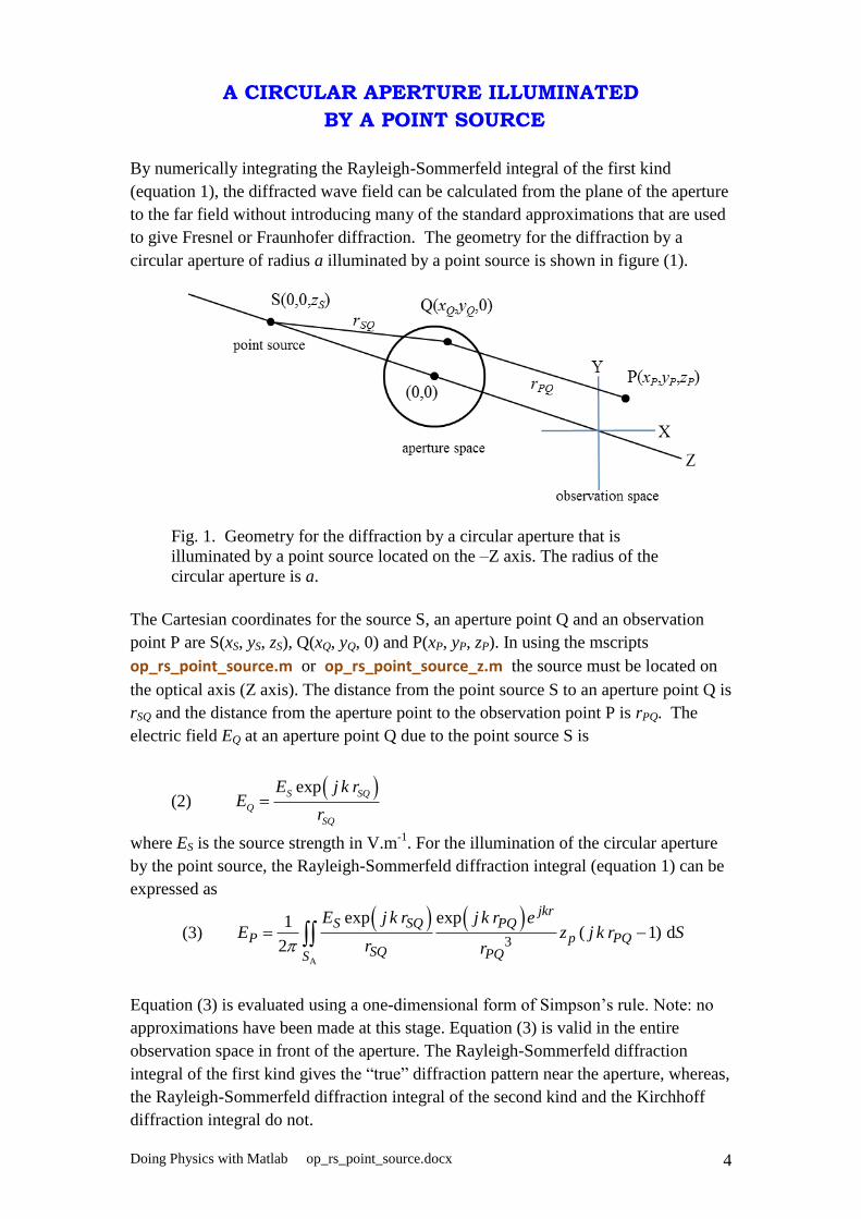
By numerically integrating the Rayleigh-Sommerfeld integral of the first kind

(equation 1), the diffracted wave field can be calculated from the plane of the aperture

to the far field without introducing many of the standard approximations that are used

to give Fresnel or Fraunhofer diffraction. The geometry for the diffraction by a

circular aperture of radius a illuminated by a point source is shown in figure (1).

Fig. 1. Geometry for the diffraction by a circular aperture that is

illuminated by a point source located on the –Z axis. The radius of the

circular aperture is a.

The Cartesian coordinates for the source S, an aperture point Q and an observation

point P are S(xS, yS, zS), Q(xQ, yQ, 0) and P(xP, yP, zP). In using the mscripts

op_rs_point_source.m or op_rs_point_source_z.m the source must be located on

the optical axis (Z axis). The distance from the point source S to an aperture point Q is

rSQ and the distance from the aperture point to the observation point P is rPQ. The

electric field EQ at an aperture point Q due to the point source S is

(2) expS SQ

Q

SQ

E j k rE

r

where ES is the source strength in V.m-1

. For the illumination of the circular aperture

by the point source, the Rayleigh-Sommerfeld diffraction integral (equation 1) can be

expressed as

(3)

A

3

exp exp1( 1) d

2

jkrS SQ PQ

P p PQSQ PQS

E j k r j k r eE z j k r S

r r

Equation (3) is evaluated using a one-dimensional form of Simpson’s rule. Note: no

approximations have been made at this stage. Equation (3) is valid in the entire

observation space in front of the aperture. The Rayleigh-Sommerfeld diffraction

integral of the first kind gives the “true” diffraction pattern near the aperture, whereas,

the Rayleigh-Sommerfeld diffraction integral of the second kind and the Kirchhoff

diffraction integral do not.

Doing Physics with Matlab op_rs_point_source.docx 5

IRRADIANCE DENSITY VARIATION ALONG THE OPTICAL AXIS

From the Rayleigh-Sommerfeld diffraction integral of the first kind (equation 3), the

axial irradiance 0,0,P PI z for a circular aperture illuminated by a plane wave can be

expressed in a simple analytical form without any approximations due to the

symmetry along the optical axis [Osterberg, Dubra]

(4)

2

2 2

2 2 2 2

20,0, 1 cos

4

Q P PP P P P

P P

I z zI z k a z z

a z a z

where IQ is the radiant flux density from the aperture. Because of the cosine term, the

axial irradiance oscillates and is bound between two envelopes corresponding to the

locus of the minima and maxima of the axial irradiance. The envelopes of the peaks

and troughs is given by

(5)

2

2 2(0,0, ) 1

4

Q PP P

P

I zI z

z a

From equation (4), peaks in the irradiance distribution along the optical axis will

occur when the cosine term is equal to zero, hence

(6) 2 2 2 1 0,1, 2, 3,2

P Pk a z z m m

Rearranging equation (6) gives the values of zP for the peaks

(7) 2 2 21

2( )0,1, 2, 3, ...

(2 1)P

a mz m

m

Since zP > 0 then

(8) 22 21 1

2 2

aa m m

For an aperture of radius a = 10 , the allowed values of m are 0, 1, 2, … , 9 giving 10

peak in the irradiance distribution along the optical axis in front of the aperture.

Doing Physics with Matlab op_rs_point_source.docx 6

To simulate a plane wave with our point source, it is only necessary to make zS very

large. We will consider a simulation with the following parameters using the mscript

op_rs_point_source_z.m

Source xS = 0, yS = 0 and zS = -1.00 m

Source Strength EQ = 1.00 V.m-1

Wavelength = 632.8 nm

Aperture radius a = 10

Aperture partitions nQ = 681701

Observation partitions nP = 1809

A typical execution time for running the mscript is about 3 minutes.

A comparison of the analytical and numerical evaluations of the diffraction integral

(equation 3) is shown in figure (2) – the top graph shows the irradiance from the near

field (Fresnel region) to the far field (Fraunhofer region) and the bottom graph shows

the near field only. There are 10 peaks in the irradiance distribution as predicted by

equation (8). The maximum irradiance occurs at an axial distance of about 100 from

the aperture and then decreases monotonically with increasing values of zP. For zP. <

100 and as zP decreases to zero as one approached the aperture, the irradiance

oscillates with increasing frequency and decreases in value to ¼ of the maximum

irradiance at the largest peak which occurs at about 100 .

How good is the Simpson’s method of evaluating the diffraction integral given by

equation (3) compared with the exact analytical evaluation of the diffraction integral

given by equation (4)? The answer is: the agreement between the numerical approach

and the analytical one is excellent as shown by the plots in figure (2) provided that the

number of partitions of the aperture and observation spaces are sufficiently large.

How large can be found by increasing the number of partitions until there is a

convergence in the results.

There are often claims in the literature that there are difficulties in performing

numerical integration of diffraction integrals because of the highly oscillatory

integrand, however, the results as indicated in figure (2), confirms the accuracy of the

numerical method using Simpson’s rule in evaluating the Rayleigh-Sommerfeld

diffraction integral of the first kind.

Doing Physics with Matlab op_rs_point_source.docx 7

Fig. 2. The irradiance distribution along the optical axis. The red curves

are for the envelopes (equation 5), the blue solid curve is the analytical

evaluation (equation 4) and the blue circles for the numerical evaluation

of equation (3) using Simpson’s rule for the double integral.

S(0, 0, - 1.00 m) op_rs_point_source_z.m

Doing Physics with Matlab op_rs_point_source.docx 8

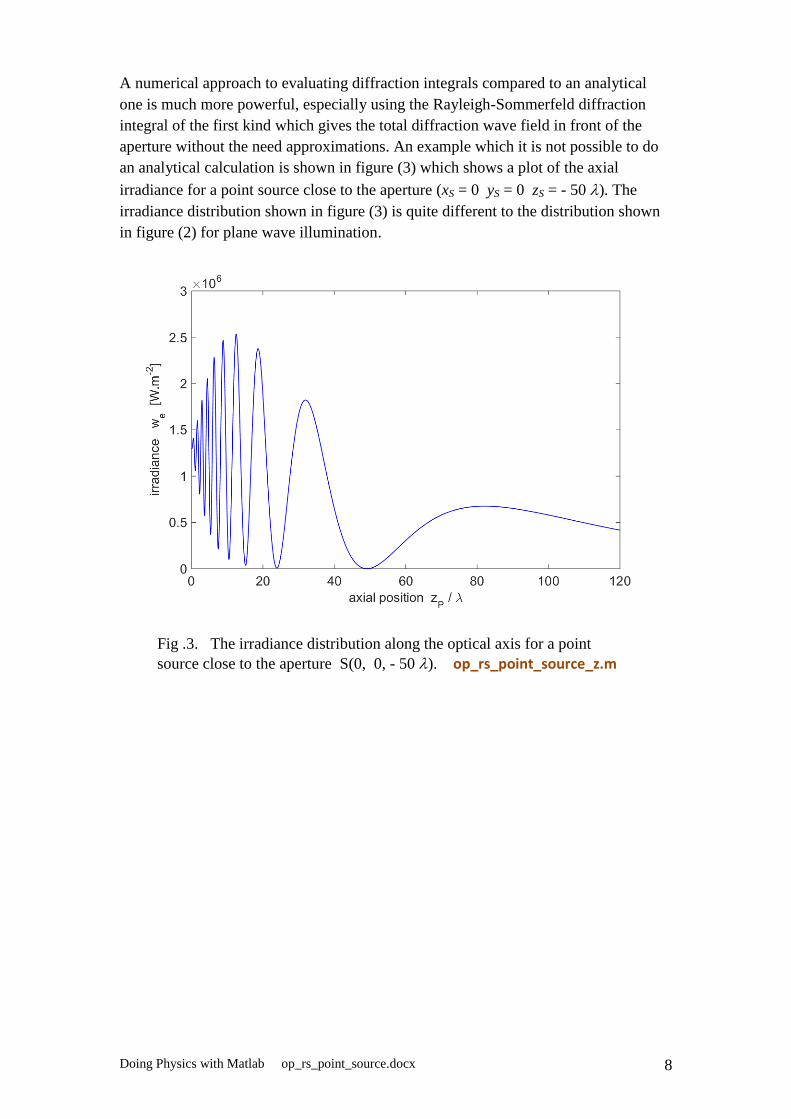
A numerical approach to evaluating diffraction integrals compared to an analytical

one is much more powerful, especially using the Rayleigh-Sommerfeld diffraction

integral of the first kind which gives the total diffraction wave field in front of the

aperture without the need approximations. An example which it is not possible to do

an analytical calculation is shown in figure (3) which shows a plot of the axial

irradiance for a point source close to the aperture (xS = 0 yS = 0 zS = - 50 ). The

irradiance distribution shown in figure (3) is quite different to the distribution shown

in figure (2) for plane wave illumination.

Fig .3. The irradiance distribution along the optical axis for a point

source close to the aperture S(0, 0, - 50 ). op_rs_point_source_z.m

Doing Physics with Matlab op_rs_point_source.docx 9

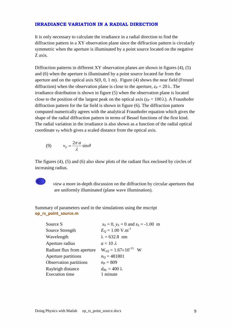
IRRADIANCE VARIATION IN A RADIAL DIRECTION

It is only necessary to calculate the irradiance in a radial direction to find the

diffraction pattern in a XY observation plane since the diffraction pattern is circularly

symmetric when the aperture is illuminated by a point source located on the negative

Z axis.

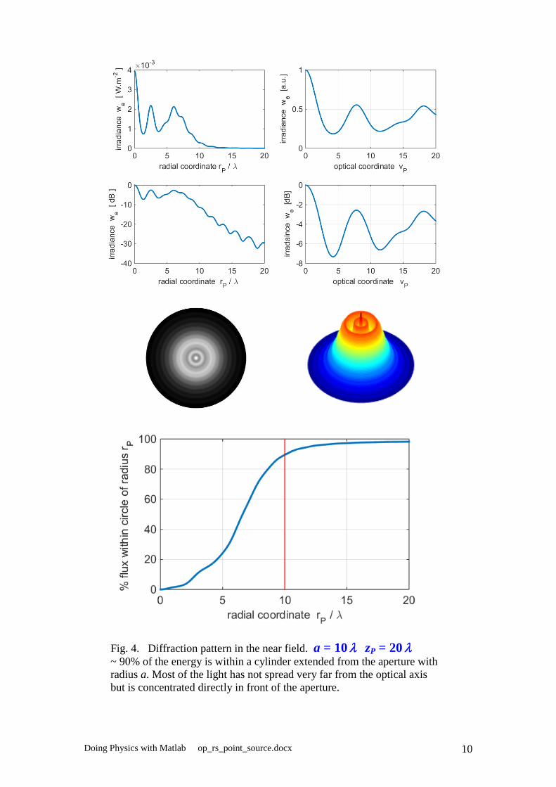
Diffraction patterns in different XY observation planes are shown in figures (4), (5)

and (6) when the aperture is illuminated by a point source located far from the

aperture and on the optical axis S(0, 0, 1 m). Figure (4) shows the near field (Fresnel

diffraction) when the observation plane is close to the aperture, zP = 20 . The

irradiance distribution is shown in figure (5) when the observation plane is located

close to the position of the largest peak on the optical axis (zP = 100 ). A Fraunhofer

diffraction pattern for the far field is shown in figure (6). The diffraction pattern

computed numerically agrees with the analytical Fraunhofer equation which gives the

shape of the radial diffraction pattern in terms of Bessel functions of the first kind.

The radial variation in the irradiance is also shown as a function of the radial optical

coordinate vP which gives a scaled distance from the optical axis.

(9) 2

sinP

av

The figures (4), (5) and (6) also show plots of the radiant flux enclosed by circles of

increasing radius.

view a more in-depth discussion on the diffraction by circular apertures that

are uniformly illuminated (plane wave illumination).

Summary of parameters used in the simulations using the mscript

op_rs_point_source.m

Source S xS = 0, yS = 0 and zS = -1.00 m

Source Strength EQ = 1.00 V.m-1

Wavelength = 632.8 nm

Aperture radius a = 10

Radiant flux from aperture WeQ = 1.6710-13

W

Aperture partitions nQ = 481801

Observation partitions nP = 809

Rayleigh distance dRL = 400

Execution time 1 minute

Doing Physics with Matlab op_rs_point_source.docx 10

Fig. 4. Diffraction pattern in the near field. a = 10 zP = 20 ~ 90% of the energy is within a cylinder extended from the aperture with

radius a. Most of the light has not spread very far from the optical axis

but is concentrated directly in front of the aperture.

Doing Physics with Matlab op_rs_point_source.docx 11

Fig. 5. Diffraction pattern in Fresnel region. a = 10 zP = 100 ~ 78% of the energy is within a cylinder extended from the aperture with

radius a. Most of the light still has not spread very far from the optical

axis but is concentrated directly in front of the aperture.

Doing Physics with Matlab op_rs_point_source.docx 12

Fig. 6. Diffraction pattern in Fraunhofer region. a = 10 zP = 600 ~ 20% of the energy is within a cylinder extended from the aperture with

radius a. Most of the light has now diffracted away from the optical axis.

Doing Physics with Matlab op_rs_point_source.docx 13

We can also model the diffraction pattern for the source close to the aperture. Figure

(7) shows the diffraction pattern for the source S(0, 0, -50).

Fig. 7. Diffraction pattern for the source close to the aperture

S(0, 0, -50). a = 10 zP = 600 . Irradiance values are very large

because the because of the close proximity of the point source to the

aperture.

Doing Physics with Matlab op_rs_point_source.docx 14

Using a purely numerical technique makes it possible to compute the diffraction field

for a much greater variety of situations than would be possible using more traditional

analytical methods. For example, the diffracted wave field can be determined for a

point source which is not located along the –Z axis.

Figures (8) and (9) show the diffraction patterns from a circular aperture of radius

a = 10 in the observation plane located at zP = 100 for a source located at

zS = -50 using the mscript op_rs_point_source_xy.m . Execution time was about 8

minutes for the partitioning of the aperture space nQ = 24341 and observation space

nPnP = 221221 = 48841. More calculations need to be done using the mscript

op_rs_point_source_xy.m because in the off-axis case one can’t make use of the

symmetry properties of the aperture and observation spaces. The plots show scaled

values of the irradiance to better emphasize the positions of the minima and maxima.

Figure (8) is for the point source on the optical axis S(0, 0, -50 ) . Figure (9) is the

example for the source located off-axis S(20 , 20 , -50 ). The diffraction pattern is

characterized by distorted circles surrounding an off-axis bright spot that has a

complex structure.

Fig. 8. The radial irradiance for the source located on the optical axis.

= 632.8 nm zP = 100 S(0, 0, -50 ). op_rs_point_source_xy.m

Doing Physics with Matlab op_rs_point_source.docx 15

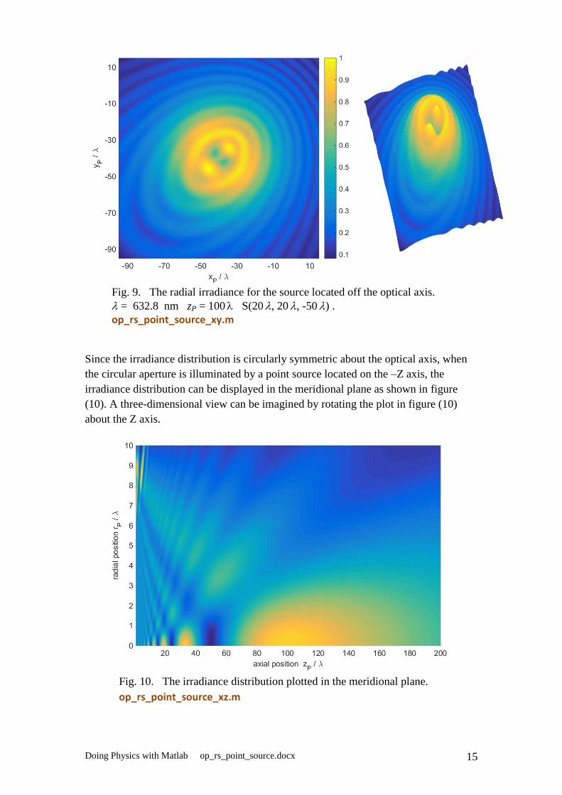
Fig. 9. The radial irradiance for the source located off the optical axis.

= 632.8 nm zP = 100 S(20 , 20 , -50 ) .

op_rs_point_source_xy.m

Since the irradiance distribution is circularly symmetric about the optical axis, when

the circular aperture is illuminated by a point source located on the –Z axis, the

irradiance distribution can be displayed in the meridional plane as shown in figure

(10). A three-dimensional view can be imagined by rotating the plot in figure (10)

about the Z axis.

Fig. 10. The irradiance distribution plotted in the meridional plane.

op_rs_point_source_xz.m

Doing Physics with Matlab op_rs_point_source.docx 16

The diffracted wave field given by the Rayleigh-Sommerfeld diffraction integral of

the first kind is valid over the whole space in front of the aperture, both close and far

from the aperture and in regions away from the axis. By having a numerical method

of integration that is both accurate and quick, one can eliminate sets of

approximations and there is no need for introducing a variety of optical coordinates

that are necessary so that the diffraction integrals can be done analytically. The

numerical procedure can be used to check many of the approximation methods that

have been used in the past. The ability to calculate the near field is also important in

investigating the behaviour of near field imaging systems.

Background documents

Irradiance and radiant flux

Scalar Diffraction theory: Diffraction Integrals

Numerical Integration Methods for the Rayleigh-Sommerfeld Diffraction

Integral of the First Kind

View: a more in-depth discussion on the diffraction by circular apertures

that are uniformly illuminated (plane wave illumination).

REFERENCES

Barakat R: The calculation of integrals encountered in optical diffraction theory. In

Frieden BR (Ed): The computer in optical research, methods and application.

pp. 35-80. Springer-Verlag, Berlin 1980

Born M, Wolf E: Principles of Optics, 7th

Ed. Cambridge University, Cambridge 1999

Cooper IJ, Sheppard CJR, Sharma M: Numerical integration of diffraction integrals

for a circular aperture. Optik, No. 7 (2002) 293-298.

Dubra A, Ferrari JA: Diffracted field by an arbitrary aperture. Am. J. Phys. 67(1)

(1999) 87-92

Forbes GW: Validity of the Frensel approximation in the diffraction of collimated

beams. J.Opt.soc.Am.A.13 (1996) 1816 – 1826

Doing Physics with Matlab op_rs_point_source.docx 17

Ganci S: Equivalence between two consistent formulations of Kirchhoff’s diffraction

theory. J. Opt. Soc. Am. A. 5 (1988) 1626 - 1628

Hsu W, Barakat R: Stratton-Chu vectorial diffraction of electromagnetic fields by

apertures with application to small-Fresnel-number systems. J.Opt.soc.Am.A.11

(1994) 623 – 629

Lindfield G, Penny: Numerical methods using Matlab. Ellishwood, New York 1995

Marchand EW, Wolf E: Consistent formulation of Kirchoff’s diffraction theory. J.

Opt. Soc. Am. A. 16 (1966) 1712 - 1722

Mendlovic D, Zalevsky Z , Konforti N: Computation considerations and fast

algorithms for calculating the diffraction integral. J.Mod.Opt. 44 (1997) 407 -

414

Osterberg H, Smith LW: Closed solutions of Rayleigh’s integral for axial points. J.

Opt. Soc. 51(10) (1961) 1050 - 1054

Pozrikidis C: Numerical computation in science and engineering. Oxford University

Press 1998

Sheppard CJR, Hrynevych M: Diffraction by a circular aperture: a generalization of

Fresnel diffraction theory. J. Opt. Soc. Am. A 9 (1992) 274 - 281

Sheppard CJR, Torok P: Effects of Fresnel number in focussong and imaging. pp. 635

– 649. In Nijhawan OP, Gupta AK, Musla AK, Singh K (Eds): Optics and

optoelectronics Vol 1, Narosa Publishing House, New Delhi 1999

Sommerfeld A: Optics – Lectures on theoretical Physics. Vol. 4, pp. 201-217.

Academic Press, London 1964

Stamnes JJ: Waves in focal regions. Adam Hilger, Bristol 1986

Steane AM, Rutt HN: Diffraction calculations in the near field and the validity of the

Fresnel approximation. J. Opt. Soc. Am. A 6 (1989) pp.1809 – 1814