MATLAB Sidebars to Accompany

MEASUREMENT AND DATA ANALYSIS FOR

ENGINEERING AND SCIENCE

Second Edition, Taylor and Francis/CRC Press, c©2010

ISBN: 9781439825686

Patrick F. Dunn

pdunn@nd.edu

107 Hessert Laboratory

Department of Aerospace and Mechanical Engineering

University of Notre Dame

Notre Dame, IN 46556

August 2009

This document presents MATLAB Sidebars that were developed for supplement the

material presented in the chapters of MEASUREMENT AND DATA ANALYSIS FOR

ENGINEERING AND SCIENCE. The Table of Contents is listed on the next page, followed

by the chapter Sidebars.

All M-files referred to herein are contained within the downloadable file “MATLAB

Files” on the text web site.

1

Contents

1 Experiments 3

2 Electronics 4

3 Measurement Systems 5

4 Calibration and Response 6

5 Probability 16

6 Statistics 28

7 Uncertainty Analysis 40

8 Regression and Correlation 45

9 Signal Characteristics 56

10 Signal Analysis 64

11 Units and Significant Figures 71

12 Technical Communication 73

2

Chapter 1

Experiments

3

Chapter 2

Electronics

4

Figure 3.1:

Chapter 3

Measurement Systems

MATLAB Sidebar 3.1The MATLAB m-file digfilt.m was written to perform low-pass digital filtering according to

Equation 3.19 in the text. It was used to generate Figure 3.1. This M-file can be adapted to receive asinput an array of discrete data.

5

Chapter 4

Calibration and Response

MATLAB Sidebar 4.1For a space-delimited array, for example Y.dat, that is contained within the same working directory,

the MATLAB command load Y.dat will bring the array into the workspace. This subsequently isreferred to as Y in the workspace. By typing Y, all the elements of that array will be displayed. AnM-file can be written to prompt the user to enter the array’s file name. This is accomplished with theMATLAB command sequence

filename = input(‘enter the file name with its extension: ’,‘s’)

eval([‘load ’,filename])

Note that a space is required after the word load in the second line. The element in the second row andthird column of that file, if it existed, would be identified subsequently by the command filename(2,3).

If a data file is located in a directory other than the current path directory, then the followingcommand sequence will change to the other directory (here its path is C:\otherdir) containing the file(here called some.dat), load the file into the workspace and then return to the original directory (hereidentified as pdir):

pdir = pwd;

cd C:\otherdir

load some.dat

eval([‘cd ’,pdir])

Note the required space after cd in the last line. This command sequence is quite useful when dealingwith many files located in different directories.

Also, the MATLAB command fscanf can be used to read formatted data from a file. Here, thefile OUT.dat would be opened or created, written to and closed using the commands:

fid = fopen(‘OUT.dat’)

myformat = ‘%g %g %g’

A = fscanf(fid,myformat,[3 inf])

A = A’

fclose(fid)

The fscanf command reads data from the file specified by an integer file identifier (fid) established bythe command fopen. Each column of data is read into the matrix A as a row according to the specifiedformat (%g allows either decimal or scientific formatted data to be read). If the specified format does notmatch the data, the file reading stops. The [3 inf] term specifies the size of A, here 3 rows of arbitrary(inf) length. The matrix A then is transposed to mirror the original column structure of OUT.dat.After these operations, the file is closed.

6

MATLAB Sidebar 4.2The MATLAB M-file plotxy.m plots the (x,y) data pairs of a user-specified data file in which the

variable values are listed in columns. The data values in any two user-specified columns can be plottedas pairs. The M-file plots the data pairs as circles with lines in between the pairs.

7

MATLAB Sidebar 4.3For situations either when a file contains some text in rows or columns that is not needed within the

workspace or when a file needs to be created without text from one that does have text, the MATLABcommand textread can be used. For example, assume that the file WTEXT.dat contains four columnsconsisting of text in columns 1 and 3 and decimal numbers in columns 2 and 4. The following commandsequence reads WTEXT.dat and then stores the decimal numbers as vectors x and y for columns 2 and4, respectively, in the workspace:

myformat = ‘\%*s \%f \%*s \%f’

[x,y] = textread(‘WTEXT.dat’,myformat)

Note that if the input file is constructed with text in the first n rows and then numbers, say threenumbers, separated by spaces in subsequent rows, the sequence of commands would be:

myformat = ‘\%f \%f \%f’

[x,y,z] = textread(‘WTEXT.dat’,myformat,‘headerlines’,n)

Remember that the format must be consistent with the variables represented by numbers in each row.

8

MATLAB Sidebar 4.4An experimentalist wishes to load a data file into the MATLAB workspace, convert some of its

information and then store that converted information in another data file. Assume that the input datafile called IN.dat consists of 4 rows of unknown length. The first row is time, the third distance andthe fourth force. Information in the second row is not needed. The desired output file will be calledOUT.dat and consists of two columns, the first time and the second work. What are the MATLABcommands needed to accomplish this?

The first task is to load the input file into the MATLAB workspace, as described before. Theneach row of data would be given its name by

time = filename(1,:);

distance = filename(3,:);

force = filename(4,:);

Next, a matrix called A is created that would have time as its first column and work, which equals forcetimes distance, as its second column. This is done by the commands

work = force.*distance

A = [time;work]

Finally, the MATLAB command fprintf can be used. Here, the file OUT.dat is opened or created,written to and finally closed using the commands

fid = fopen(‘OUT.dat’,’wt’)

myformat = ‘%12.6f %12.6f\n’

fprintf(fid,myformat,A)

fclose(fid)

The letters wt in the second line create a file in the text mode (t) to which the data can be written(w). The \n in the third line starts the next row. The %12.6f sets the number’s format to decimalformat and stores the number as 12 digits, with 6 digits to the right of the decimal point. Alternatively,scientific format (%e) can be used. Specifying the format %g allows MATLAB to choose either decimalor scientific format, whichever is shorter.

9

Figure 4.1:

MATLAB Sidebar 4.5The MATLAB M-file fordstepmd.m was used to generate Figure 4.1. It determines both the

magnitude ratio and the dynamic error of a first-order system’s response to a step-input forcing as afunction of the dimensionless time.

10

Figure 4.2:

Figure 4.3:

MATLAB Sidebar 4.6The MATLAB M-files fordsineM.m and fordsinep.m plot the steady-state first-order system’s

magnitude ratio and phase lag, respectively, in response to sinusoidal-input forcing. These are plot-ted versus the dimensionless parameter ωτ . Figures 4.2 and 4.3 were made using fordsineM.m andfordsinep.m, respectively.

11

Figure 4.4:

Figure 4.5:

MATLAB Sidebar 4.7The MATLAB M-file secordstep.m this plots second-order system response to step-input forcing.

It accepts a user-specified value of ζ. This M-file was used to create Figures 4.4 and 4.5. For convenience,the natural frequency is set equal to 1 in the M-file, but can be changed.

12

Figure 4.6:

MATLAB Sidebar 4.8When examining the response of a system to an input forcing, often one is interested in finding the

time it takes for the system finally to reach a steady-state value to within some percentage tolerance.The MATLAB M-file sstol.m accomplishes this task. This M-file uses the MATLAB command break

in the conditional loop

if abs((x(i)-meanx)>delxtol)

tsave=t(i+1);

j=i;

break

end

which causes the program to exit the conditional loop and save the time at which the difference betweenx and its mean value exceeds a certain tolerance.

Figure 4.6 was produced by sstol.m for the case of a second-order system with a damping coefficientequal to 0.3 in response to step-input forcing. This M-file is constructed to receive a user-specified inputdata file that consists of two columns, time and amplitude. The percent plus-minus tolerance alsois user-specified. The M-file also indicates the time at which the signal reaches and stays within thetolerance limit. The figure label lists values of the steady-state mean amplitude, the time at which thesignal stays within the specified tolerance and the tolerance percentage. The time to reach steady-stateactually is determined by examining the data file in reverse order. This way, it is simple to determinethe tolerance time by finding when the amplitude first exceeds the tolerance level.

13

Figure 4.7:

Figure 4.8:

MATLAB Sidebar 4.9The MATLAB M-files secordsineM.m and secordsinep.m plot the steady-state second-order

system’s magnitude ratio and phase lag, respectively, in response to sinusoidal-input forcing. BothM-files accept user-specified values of ζ. Figures 4.7 and 4.8 were made using secordsineM.m andsecordsinep.m, respectively.

14

MATLAB Sidebar 4.10MATLAB can be used to numerically integrate first-order ordinary differential equations. The M-

file odeint.m numerically integrates and plots a user-specified first-order ordinary differential equationover a user-specified range of the independent variable. The results of four methods (forward Euler,backward Euler, improved Euler and 4th-order Runge-Kutta) are plotted and compared with the exactresult. MATLAB also has the built-in functions ode23 and ode45 that perform numerical integrationusing mixed-order Runge-Kutta methods.

15

Chapter 5

Probability

MATLAB Sidebar 5.1MATLAB works well with user-defined functions. In a user-defined function, input and output

variables can be specified, as is done by the subroutine of a computer program. The general form of aMATLAB function is function [output1, output2, ...] = functionname(input1, input2, ...). The functionis saved as a MATLAB M-file and then referred to in another M-file or active workspace by its namewith values given for its arguments. For example, the user-defined function called triprob (stored astriprob.m within the directory) is defined as

function [w] = triprob(x,y,z)

w = x*y*z

When the function is referred to by a statement such as “triprob(0.3,0.4,0.5);” that includes a semi-colon, the output will be displayed with the the variable name stated within the function’s M-file. Forthis case, it would be “w = 0.06.”

16

MATLAB Sidebar 5.2MATLAB can be used to determine the values of n!, P n

m, Cnm and Cn

m(r) using a simple “for”loop to determine the factorial of a number. This is accomplished by decrementing the loop from thespecified value of n down to a value of 2 by -1 while forming the product of the decremented numbers.For example, to compute n!, it would be written in MATLAB script:

x = 1;

for i = n:-1:2

x = i*x

end

nfac = x

The user-defined function pandc.m computes n!, P nm, Cn

m and Cnm(r). Its arguments are n and m. With

pandc.m in the MATLAB workspace, simply typing pandc(n,m) will list the desired four values. As anexample, typing pandc(4,3) returns the values 24, 24, 4 and 20, corresponding to 4!, P 4

3 , C43 and C4

3(r),respectively.

17

Figure 5.1:

MATLAB Sidebar 5.3Figure 5.1 was constructed using the MATLAB M-file signals.m. The data for the solid curve

was generated by creating an array of 1000 points from 0 to 10 and the corresponding magnitudes (yvalues) by the commands:

t = 0:0.01:10;

ycont = 10*(1+0.2*sin(0.3*t)+0.1*cos(1.5*t))-9;

Strictly speaking, this results in a discrete signal. But because of the small increments in t, it will appearas a continuous signal in the figure. The discrete signal consists of 10 points found by the commands:

td = 0:1:10;

ydisc = 10*(1+0.2*sin(0.3*td)+0.1*cos(1.5*td))-9;

The digital signal was obtained by directly entering an array of magnitudes after rounding off the discretevalues to the nearest 0.5:

ydig = [1.5,1.0,2.5,4.0,3.5,2.0,2.5,3.0,2.5,0.5];

These values also can be determined using MATLAB’s round command.The resulting plot was constructed as a series of three overlay plots because the magnitude arrays

have different sizes. This was done using MATLAB’s hold on command as follows:

plot(t,ycont,’k’)

hold on

plot(td,ydisc,’kx’)

hold on

plot(td,ydig,’ko’)

If each of the t and y arrays were the same size, then the plot could be made using one command line:

plot(t,ycont,’k’,td,ydisc,’kx’,td,ydig,’ko’)

18

MATLAB Sidebar 5.4Data that is stored in files can be read easily using MATLAB commands. The following series

of MATLAB commands asks the user to identify a data file, which then is read into the MATLABworkspace by the commands:

filename = input(’enter the filename w/o its extension: ’,’s’);

ext = input(’enter the files extension, e.g., dat: ’,’s’);

num = input(’enter the column number of the data to plot (e.g., 1): ’);

eval([’load ’,filename,’.’,ext]);

The number of rows and columns of the data array can be determined by the command:

[rows,cols] = size(eval([filename,’(:,1)’]));

Part or all of a particular column of the array can be named. For example, say that the data file wasnamed testone.dat. Assume that the first two rows of each column are text identifiers that name thevariable and its units. The third row and beyond is the actual data. If the first column were pressuredata, then the actual data could be identified using the statement:

pressure = testone(3:length(testone),1);

The MATLAB length command determines the number of rows. The argument 3:length(testone)

identifies the third through last rows and the argument 1 the first column. The arguments 3:rows,1

would do the same for this case. Such commands can be embedded into the beginning of an M-file thatis written to analyze and plot data.

19

Figure 5.2:

MATLAB Sidebar 5.5The M-file 3histos.m was used to construct Figure 5.2. It reads data from a user-specified file and

then plots three histograms side by side. The number of intervals for each of the three histograms isuser-specified. Theoretical values are generated by specifying the distribution of the population, whichcurrently is set in the M-file to be the normal distribution.

20

MATLAB Sidebar 5.6The MATLAB M-file mw.m calculates the factor c and K of the Mann and Wald formula for user-

specified values of the % level of significance (= 100 % - % confidence) and N. As an example, for N =250 and 10 % level of significance, mw.m determines c = 1.2816 and K = 18.

21

Figure 5.3:

MATLAB Sidebar 5.7The MATLAB M-file kforN.m was used to construct Figure 5.3. The range of N can be varied by

the user.

22

MATLAB Sidebar 5.8The M-file histo.m plots the equal-width interval histogram of a selected column from a user-

specified data file. Scott’s formula is used for K although other formulas are provided. The MATLABcommand “[cnts,binloc] = hist(data,k)” determines the number of counts “cnts” in each of “k” intervalsfrom the array “data”. The abscissa position for each interval is specified by the array “binloc.” Thecommand “bar(binloc,cnts)” plots the histogram.

23

Figure 5.4:

MATLAB Sidebar 5.9The M-file hf.m plots the histogram and frequency distribution of a selected column of data. The

frequency distribution is obtained by the MATLAB command “bar(binloc,cnts/N)” after determiningthe “binloc” and “cnts” arrays using MATLAB’s “hist” command. An example of the resulting figurefor a data array of 2564 measurements is shown in Figure 5.4.

24

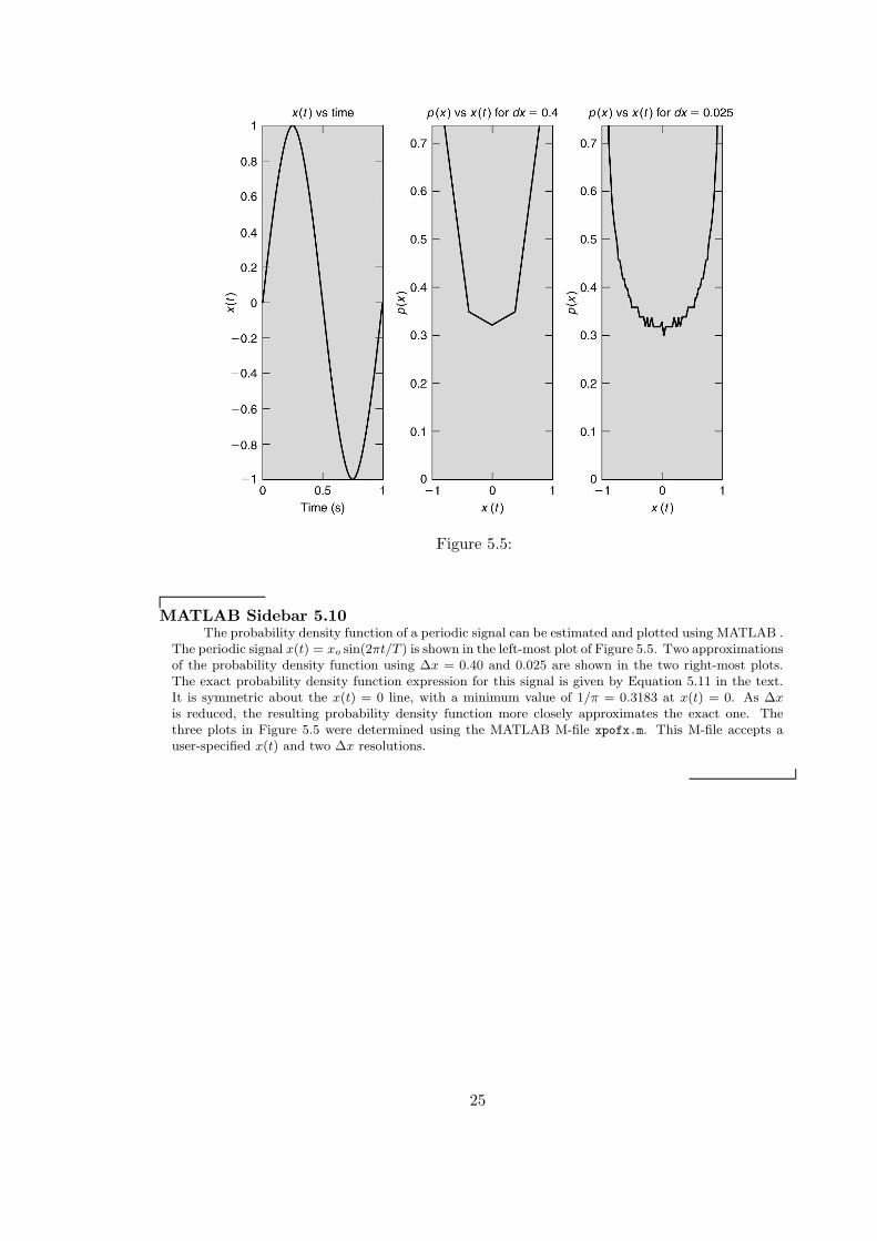
Figure 5.5:

MATLAB Sidebar 5.10The probability density function of a periodic signal can be estimated and plotted using MATLAB .

The periodic signal x(t) = xo sin(2πt/T ) is shown in the left-most plot of Figure 5.5. Two approximationsof the probability density function using ∆x = 0.40 and 0.025 are shown in the two right-most plots.The exact probability density function expression for this signal is given by Equation 5.11 in the text.It is symmetric about the x(t) = 0 line, with a minimum value of 1/π = 0.3183 at x(t) = 0. As ∆xis reduced, the resulting probability density function more closely approximates the exact one. Thethree plots in Figure 5.5 were determined using the MATLAB M-file xpofx.m. This M-file accepts auser-specified x(t) and two ∆x resolutions.

25

MATLAB Sidebar 5.11The MATLAB command moment(X,m) determines the m-th central moment of the vector X.

The second central moment is calculated using a divisor of N instead of N-1 where N is the sam-ple size. The variance is moment(X,2), the skewness moment(X,3)/moment(X,2)1.5 and the kurtosismoment(X,4)/moment(X,2)2. As an example, for X = [1, 2, 3, 4, 5, 6, 7, 8, 9], moment(X,2) = 6.6667, mo-ment(X,3) = 0 and moment(X,4) = 78.6667. This yields σ2 = 6.6667, Sk = 0 and Ku = 78.6667/6.66672

= 1.7700.MATLAB also has many functions that are used to statistically quantify a set of numbers. Infor-

mation about any MATLAB function can be obtained by simply typing help xxx, where xxx denotesthe specific MATLAB command. The MATLAB command mean(X) provides the mean of the vectorX. If the matrix called data has more than one column, then each column can be vectorized usingthe statement X(i) = data(:,i), which assigns the vector X(i) the elements in the i-th column of thematrix data. Subsequently, one can find the minimum value of X(i) by the command min(X(i)), themaximum by max(X(i)), the standard deviation by std(X(i)), the variance by [std(X(i))]^2 and theroot-mean-square by norm(X(i))/sqrt(N). The command norm(X(i),p) is the same as the commandsum(abs(X(i)).^p)^(1/p). The default value of p is 2 if a value for p is not entered into the argumentof norm. Thus, norm(X(i)) is the same as norm(X(i),2).

26

MATLAB Sidebar 5.12The user-defined function stats.m computes the values of the following statistics of the vector X:

number of values, minimum, maximum, mean, standard deviation, variance, root-mean-square, skewnessand kurtosis. The MATLAB commands skewness(X) and kurtosis(X) are used to compute theirvalues. For the vector X specified in the previous Sidebar, typing stats(X) results in the followingvalues: number = 9, minimum = 1, maximum = 9, mean = 5 , standard deviation = 2.7386, variance= 7.5000, rms = 5.6273, skewness = 0 and kurtosis = 1.7700.

27

Chapter 6

Statistics

MATLAB Sidebar 6.1The probability density and distribution functions for many common statistical distributions are

available via MATLAB’s statistics toolbox. These include the binomial (bino), Poisson (poiss), Normal(norm), Chi-square (chi2), lognormal (logn), Weibull (weib), uniform (unif) and exponential (exp) dis-tributions. Three MATLAB commands used quite often are pdf, cdf and inv, denoting the probabilitydensity, cumulative distribution and inverse functions, respectively. MATLAB provides each of thesefunctions for specific distributions, where different input arguments are required for each distribution.These functions carry a prefix signifying the abbreviated name of the distribution, as indicated above,and the suffix of either pdf, cdf or inv. For example, normpdf is the Normal distribution probabilitydensity function. MATLAB also provides generic pdf and cdf functions for which one of the function’sarguments is the abbreviated name of the distribution. A word of caution: in MATLAB the symbolP denotes the integral of the probability density function from -∞ to the argument of P . In this textthe meaning of P sometimes is different. P (x) (see Equation 6.6 in the text) denotes the integral ofthe probability density function from - the argument of P to + the argument of P , whereas P (x∗) (seeEquation 5.28 in the text) has the same meaning as in MATLAB .

28

MATLAB Sidebar 6.2MATLAB’s statistics toolbox contains a number of commands that simplify statistical analysis.

Two tools, disttool and randtool, are easy to use. disttool plots the probability density and distri-bution functions for any one of 19 of the most common distributions. randtool generates a frequencydensity plot for a user-specified number of samples drawn randomly from any one of these distributions.In both tools, the mean and the standard deviation of the distribution are user-specified.

29

MATLAB Sidebar 6.3The MATLAB command binopdf(n,N,P) computes the binomial probability density function

value for getting n successes with success probability P for N repeated trials. For example, the com-mand binopdf(5,10,0.5) yields the value 0.1762. That is, in a fair coin toss experiment, there isapproximately an 18 % chance that there will be exactly 5 heads in 10 tosses.

30

MATLAB Sidebar 6.4The normal distribution-specific pdf function has three arguments: a particular x-value at which

you seek the pdf value, the mean value of the distribution and the standard deviation of the distribution.For example, the MATLAB command normpdf(x,xmean,sigma) returns the value of the probabilitydensity function, p(x), evaluated at the value of x of a normal probability distribution having a meanof xmean and a standard deviation of sigma. Specifically, typing the MATLAB command normpdf(2,

0, 1) yields p(2) = 0.0540. A similar result can be obtained using the generic MATLAB commandpdf(norm, 2, 0, 1).

The normal distribution cdf function also has similar arguments: a particular x-value at whichyou seek the cdf value, the mean value of the distribution and the standard deviation of the distribution.This is none other than the integral of the pdf function from −∞ to x∗, P (x∗). So, typing the MATLABcommand normcdf(1, 0, 1) gives P (1) = 0.8413. This says that 84.13 % of all normally-distributedvalues are between −∞ and one standard deviation above the mean. Typing cdf(norm, 1, 0, 1) yieldsthe same value.

The normal distribution inv function gives the inverse of the cdf function It provides the value ofx∗ for the cdf value of P . Thus, typing the MATLAB command norminv(0.9772, 0, 1) results in thevalue of 2. This says that 97.72 % of all normally-distributed values are below two standard deviationsabove the mean. There is not an equivalent generic MATLAB inv command.

31

MATLAB Sidebar 6.5The MATLAB command normspec([lower,upper],mu,sigma) generates a plot of the normal

probability density function of mean mu and standard deviation sigma with the area shaded under thefunction between the value limits lower and upper. It also determines the percent probability of havinga normally distributed value between these limits.

32

MATLAB Sidebar 6.6To obtain a value of the normal error function, p(z1), use MATLAB’s cdf function. This is specified

by

P (z1) = normcdf (z1, 0, 1) − 0.5.

Recall that normcdf is the integral of the normal probability density function from −∞ to x∗, or to z1

in this case. Because the normal error function is defined between the limits of a normal mean equal tozero and z1, a value of 0.5 must be subtracted from normcdf to obtain the correct normal error functionvalue. (Why 0.5?) For example, typing the MATLAB command normcdf(1.37,0,1) - 0.5 returns thecorrect normal error function value of 0.4147.

33

MATLAB Sidebar 6.7The MATLAB command cdf can be used to determine the probability, P (z), that a normally

distributed value will be between ±z. This probability is determined by

P (z) =

∫ z

−∞

p(x)dx −

∫

−z

−∞

p(x)dx = normcdf (z, 0, 1) − normcdf (−z, 0, 1) .

Using this formulation, P (2) = 0.9545. That is, 95.45 % of all normally distributed values bebetween z = ±2. Further, recalling that MATLAB’s P (z) denotes the inv value from −∞ to z, aparticular value of −z can be obtained by typing the command normcdf( 1−P

2, 0, 1) and of +z by

norminv( 1+P2

, 0, 1). For example, typing the command norminv( 1−0.95452

, 0, 1) gives the z-value of -

2.00. A similar approach can be taken to find P for other distributions.

34

Figure 6.1:

MATLAB Sidebar 6.8The MATLAB M-file tz.m was used to generate Figure 6.1. This M-file utilizes the MATLAB

commands normpdf and tpdf. The M-file can be configured to plot Student’s t probability densityfunctions for any number of degrees of freedom.

35

Figure 6.2:

MATLAB Sidebar 6.9The MATLAB M-file tzcompare.m determines the percent difference in the probabilities between

the normal and Student’s t distributions that occurs with various degrees of freedom. This M-file utilizesMATLAB’s cdf command. Figure 6.2 was made using this M-file.

36

MATLAB Sidebar 6.10The MATLAB functions tpdf, tcdf and tinv are used for Student’s t distribution. The MATLAB

command tpdf(t,ν) returns the value of the probability density function, p(t, ν), evaluated at thevalue of t of Student’s t distribution having ν degrees of freedom (recall that there are an infinitenumber of Student’s t distribution, one for each degree of freedom value). Specifically, typing theMATLAB command tpdf(2, 1000) yields at value of 0.0541. Compare this to normpdf(2, 0, 1),which gives the value of 0.0540. This shows that the probability density function value for Student’st distribution for a very large number (here 1000) of degrees of freedom is effectively the same as thatof the normal distribution. However, for a low value of the number of degrees of freedom, say equal to2, the probability density function value of Student’s t distribution differs significantly from its normaldistribution counterpart (tpdf(2, 2) yields a value of 0.0680).

Exercises similar to those performed for the normal distribution can be done for Student’s t dis-tribution. Typing tcdf(1, 1000) gives the value of 0.8412 (compare this to the normal distributionvalue). Typing tinv(0.9772, 1000) results in the value of 2.0016 (again, compare this to the normaldistribution value). Finally, typing tinv( 1+0.9545

2, 1000) yields a value of 2.0025. This tells us that

95.45 % of all Student’s t-distributed values be between ±2.0025 standard deviations from the mean ofthe distribution.

37

MATLAB Sidebar 6.11The MATLAB commands chi2pdf, chi2cdf and chi2inv are used for Chi-square distribution.

MATLAB’s command chi2pdf(chisq,nu) returns the value of the probability density function, p(χ2, ν),evaluated at the value of χ2 of the Chi-square distribution having a ν degrees of freedom. Note that,like for Student’s t distribution, there are an infinite number of Chi-square distributions. Typing theMATLAB command chi2pdf(10,10) yields a value of 0.0877. Typing chi2cdf(10,10) gives a valueof 0.5595, signifying that 55.95 % of all Chi-square-distributed values for 10 degrees of freedom bebetween 0 and 10 (recall that there are no negative Chi-square values). Or, in other words, there is a44.15 % chance of finding a value greater than 10 for a 10-degree-of-freedom Chi-square distribution.Similar to other specific-distribution inv functions, chi2inv(P,ν) returns the χ2 value where betweenit and 0 are P % of all the ν-degree-of-freedom Chi-square distribution values. For example, typingchi2inv(95.96,4) yields a value of 10.

38

Figure 6.3:

MATLAB Sidebar 6.12A χ2 analysis of data can be performed automatically. The MATLAB M-file chinormchk.m does

this. This M-file reads a single-column data file and plots its frequency density distribution using Scott’sformula for equal-width intervals. It also determines the corresponding values of the normal probabilitydensity function based upon the mean and standard deviation of the data and then it plots them onthe same graph. Finally, it performs a χ2 analysis that yields the percent confidence that the expecteddistribution is the correct one.

An example of the analysis of 500 test scores using chinormchk.m is shown in Figure 6.3. Themean of the test scores was 6.0 and the standard deviation was 1.0. The analysis shows that there is a19 % chance that the scores represent those drawn from a normal distribution. This is based upon thevalues of χ2 = 8.7 and ν = 6.

39

Figure 7.1:

Chapter 7

Uncertainty Analysis

MATLAB Sidebar 7.1Experimental results can be plotted with x and y error bars using the MATLAB M-file ploterror.m.

This M-file uses a MATLAB M-file eplot.m written by Andri M. Gretarsson to draw error bars in boththe x- and y-directions. The MATLAB command errorbar only draws an error bar in the y-direction.ploterror.m reads a four-column text file of x, x -error, y and y-error values. It plots x,y error barscentered on each data point, like that shown in Figure 7.1.

40

MATLAB Sidebar 7.2The previous problem can be solved by the MATLAB M-file uncerte.m. This M-file uses MAT-

LAB’s function diff(x,y) that symbolically determines the partial derivative of x with respect to y. Amore general M-file that determines the uncertainty in a result can be constructed using this format.First, the symbols for the measured variables are declared and the expression for the result is providedby the commands

syms ha hb

e=sqrt(hb/ha);

Next, typical values for the variables and the elemental uncertainties are given. Then the uncertaintyexpression is stated in terms of the diff function:

u_e=sqrt((diff(e,ha)*u_ha).^2+diff(e,hb)*u_hb).^2);

Finally, the uncertainty is computed using successive substitutions

u_e_1=subs(u_e,ha,s_ha);

uncertainty_in_e=subs(u_e,hb,s_hb);

in which the typical values sha and shb are substituted for ha and hb, respectively. The result obtainedis ue = 7.1589E − 04, which agrees with that calculated in the previous example.

41

MATLAB Sidebar 7.3Determining the uncertainty in a result that depends upon a number of elemental uncertainties

often is tedious and subject to calculational error. One alternative approach is to expand an M-file, suchas uncerte.m, to include more than a couple of elemental errors. The MATLAB M-file uncertvhB.m waswritten to determine the velocity of a pendulum at the bottom of a swing (this is part of the laboratoryexercise on Measurement, Modeling and Uncertainty). The velocity is a function of seven variables.Such an M-file can be generalized to handle many uncertainties.

42

Figure 7.2:

MATLAB Sidebar 7.4The MATLAB M-file differ.m numerically differentiates one user-specified variable, y, with respect

to another variable, x, using the MATLAB function diff. The diff function computes the first-order,forward-difference of a variable. The derivative of y = f(x) is then determined as diff(y)/diff(x).The M-file is constructed to receive a user-specified data file from which two columns are specified asthe variables of interest. It plots the ∆y/∆x and y values versus the x values. An example output ofinteg.m is shown in Figure 7.2, in which nine (x,y) pairs comprised the data file.

43

Figure 7.3:

MATLAB Sidebar 7.5The MATLAB M-file integ.m numerically integrates one user-specified variable, y, with respect to

another variable, x, using the MATLAB function trapz(x,y). The trapz function sums the areas of thetrapezoids that are formed from the x and y values. The M-file is constructed to receive a user-specifieddata file from which two columns are specified as the variables of interest. It plots the data and liststhe value of calculated area. More accurate MATLAB functions, such as quad and quad8, performintegration using quadrature methods in which the intervals of integration are varied. An exampleoutput of integ.m is shown in Figure 7.3, in which nine (x,y) pairs comprised the data file.

44

Figure 8.1:

Chapter 8

Regression and Correlation

MATLAB Sidebar 8.1The MATLAB command p = polyfit(x,y,m) uses least-squares regression analysis on equal-

length vectors of [x,y] data to find the coefficients, a0 through am, of the polynomial p(x) = amxm +am−1x

m−1 + ...a1x + a0 and places them in a row vector p of descending order. The polynomial p isevaluated at x = x∗ using the MATLAB command polyval(p,x*). These commands, when used inconjunction with MATLAB’s plot command, allow one to plot the data along with the regression fit,as was done to construct Figure 8.1.

45

MATLAB Sidebar 8.2Usually, when applying regression analysis to data, the number of data points exceeds the number

of regression coefficients, as N > m + 1. This results in more independent equations than there areunknowns. The system of equations is overdetermined. Because the resulting matrix is not square,standard matrix inversion methods and Cramer’s method will not work. An exact solution may or maynot exist. Fortunately, MATLAB can solve this set of equations implicitly, yielding either the exactsolution or a least-squares solution. The solution is accomplished by simply using MATLAB’s matrixdivision operator (\). This operator uses Gaussian elimination as opposed to forming the inverse of thematrix. This is more efficient and has greater numerically accuracy. For N [xi, yi] data pairs there willbe N equations to evaluate, which in expanded matrix notation are

1 x1 x21 · · · xm

1

1 x2 x22 · · · xm

2

......

.... . .

...1 xN x2

N · · · xmN

a0

a1

a2

...am

=

y1

y2

y3

...yN

.

In matrix notation this becomes [X][a] = [Y ], where [X ] is a (N x m+1) matrix, [a] a (m+1 x 1) matrixand [Y ] a (N x 1) matrix. The solution to this matrix equation is achieved using the command X\Yafter the matrices [X] and [Y ] have been entered.

46

MATLAB Sidebar 8.3The MATLAB M-file plotfit.m performs an m-th order least-squares regression analysis on a set

of [x, y, ey ] data pairs (where ey is the measurement error) and plots the regression fit and the P %confidence intervals for the yi estimate. It also calculates Syx and plots the data with its error bars.

47

Figure 8.2:

MATLAB Sidebar 8.4The MATLAB M-file calexey.m performs a linear regression analysis based on Deming’s method

on a set of [x,y,ex,ey ] data pairs (where ex and ey are the measurement errors in the x and y, respectively)and plots the regression fit. It also plots the data with their measurement error bars and calculates thevalue of λ and the final estimates of the uncertainties in x and y, as given by Equations 8.53 and 8.54in the text. This was used to generate Figure 8.2.

48

Figure 8.3:

MATLAB Sidebar 8.5The MATLAB M-file confint.m performs a linear least-squares regression analysis on a set of

[x,y,ey ] data pairs (where ey is the y-measurement error) and plots the regression fit and the associatedconfidence intervals as given by Equations 8.28 through 8.30 in the text. This was used to generateFigure 8.3 for the data set given in the previous example.

49

Figure 8.4:

Figure 8.5:

MATLAB Sidebar 8.6The MATLAB M-file caley.m performs a linear least-squares regression analysis on a set of [x,y,ey ]

data pairs (where ey is y-measurement error) and plots the regression fit and the associated confidenceintervals as given by Equations 8.30 and 8.31 in the text. This was used to generate Figures 8.4 and8.5.

50

Figure 8.6:

Figure 8.7:

MATLAB Sidebar 8.7The MATLAB M-file caleyII.m determines the range in the x-from-y estimate for a user-specified

value of y in addition to those tasks done by the MATLAB M-file caley.m. This is accomplished byusing Newtonian iteration to solve for the xlower and xupper estimates that are shown in Figure 8.6.The MATLAB M-file caleyIII.m extends this type of analysis one step farther by determining thepercent uncertainty in the x-from-y estimate for the entire range of y values. It plots the standardregression fit with the data and also the x-from-y estimate uncertainty versus x. These two plots areshown in Figure 8.7.

51

MATLAB Sidebar 8.8In many experimental situations, the number of data points exceeds the number of independent

variables, leading to an overdetermined system of equations. Here, as was the case for higher-orderregression analysis solutions, MATLAB can solve this set of equations, using MATLAB’s left-divisionmethod. For N [xi, yi, zi, Ri] data points there will be N equations to evaluate, which in expandedmatrix notation are

1 x1 y1 z1

1 x1 y2 z2

......

......

1 xN yN zN

a0

a1

a2

a3

=

R1

R2

R3

...RN

.

In matrix notation this becomes [G][a] = [R], where [G] is a (N x 4) matrix, [a] a (4 x 1) matrix and[R] a (N x 1) matrix. The solution to this matrix equation is achieved using the command G\R afterthe matrices [G] and [R] have been entered.

52

MATLAB Sidebar 8.9The M-file corrprob.m and its associated function-file f1.m calculates the probability PN (| r |≥|

ro |). The definite integral is found using the quad8 function, which is an adaptive, recursive, Newton-Cotes 8-panel method. As an example, for N = 6 and ro = 0.979 corrprob.m gives PN = 0.1 %. Thus,the correlation is very significant.

53

Figure 8.8:

MATLAB Sidebar 8.10The MATLAB M-file plotPN.m constructs a plot of PN (| r |≥| ro |) versus the number of mea-

surements, N, for a user-specified value of ro. By using MATLAB’s holdon command, a figure such asFigure 8.8 can be generated for various values of ro.

54

Figure 8.9:

MATLAB Sidebar 8.11The MATLAB M-file sigcor.m determines and plots the autocorrelations and cross-correlation of

discrete data that is user-specified. The file contains an arbitrary length of time, x and y values in threecolumns. This M-file uses MATLAB’s xcorr command. The command xcorr(x,‘flag’) performs theautocorrelation of x and the command xcorr(x,y,’flag’) calculates the cross-correlation of x with y.The argument ‘flag’ of xcorr permits the user to specify how the correlations are normalized. The M-filesigcor.m uses the argument ‘coeff’ to normalize the correlations such that the autocorrelations at zerotime lag are identically 1.0. An example plot generated by sigcor.m for a file containing 8 sequentialmeasurements of x and y data is shown in Figure 8.9. Note that both autocorrelations have a value of1.0 at zero time lag.

55

Chapter 9

Signal Characteristics

MATLAB Sidebar 9.1MATLAB has a number of built-in functions that generate standard signals, such as square, trian-

gular and sawtooth waves, and the trigonometric functions. A square wave with a frequency of f Hertzand an amplitude that varies from -A to +A over the time period from 0 to 7 s is generated and plottedusing the MATLAB command sequence

t = 0:0.001:7;

sq = A*square(2*pi*f*t);

plot(t,sq)

The MATLAB sawtooth(t,width) function produces a sawtooth wave with period 2*pi. The fraction ofthe period at which sawtooth’s peak occurs is specified its width argument, whose value varies between0 and 1. A triangle wave is produced when width equals 0.5. A sawtooth wave with a period of 2*pi,its peak occurring at 0.25*2*pi and an amplitude that varies from -A to +A over the time period from0 to 7 s is generated and plotted using the MATLAB command sequence

t = 0:0.001:7;

sw = A*sawtooth(t,0.25);

plot(t,sw)

56

Figure 9.1:

MATLAB Sidebar 9.2In some instances, the amount of time that a signal resides within some amplitude window needs

to be determined. The MATLAB M-file epswin.m can be used for this purpose and to determine thetimes at which the signal’s minimum and maximum amplitude occur. Figure 9.1 was generated byepswin.m applied to the case of a pressure transducer’s response to an oscillating flow field. The M-fileis constructed to receive a user-specified input data file that consists of two columns, time and amplitude.The amplitude’s window is established by a user-specified center amplitude and an amplitude percentage.epswin.m plots the signal and indicates the percentage of the time that the signal resides within thewindow. The number of instances that the amplitude is within the window is determined using analgorithm based upon an array whose values are negative when the amplitude is within the window.The times at which the signal reaches its minimum and maximum amplitudes also are determined andindicated.

57

Figure 9.2:

MATLAB Sidebar 9.3The MATLAB M-file propintime.m was used to generate Figure 9.2. It is constructed to read

a user-specified data file and plot the values of the data’s mean, variance, skewness and kurtosis forvarious sample periods. This M-file can be used to determine the minimum sample time required toachieve statistical property values within acceptable limits.

58

Figure 9.3:

MATLAB Sidebar 9.4The M-file acdc.m was used to generate Figure 9.3. A period of time from t = 0 to t = 2

in increments of 0.02 is established first. Then y(t) is computed for that period. The mean value isdetermined next using the MATLAB mean command. This is the dc component. Then the ac componentis determined by subtracting the mean from the signal. Finally the ac component is amplified by a factorof 10. The following syntax is used as part of the M-file:

t=[0:0.02:1];

y=3+rand(size(t));

dc=ones(size(t))*mean(y);

ac=y-dc;

z=10*ac;

59

MATLAB Sidebar 9.5The rms can be computed using the MATLAB norm command. This expression norm(x) equals

sum(abs(x).2)(1/2). The “.” is present in this expression because of the multiplication of the vector x

with itself. So, the rms for the discrete signal x can be written in MATLAB as

rms=norm(x)/sqrt(length(x));

60

Figure 9.4:

MATLAB Sidebar 9.6The M-file fsstep.m was used to construct Figure 9.4. This M-file uses the MATLAB symsum

command to create the sum of the Fourier series. This is accomplished in part for the sum of 500harmonics shown in the figure by the syntax

syms n t

y=(10/(n*pi))*(1-cos(n*pi))*sin(n*t);

step=symsum(y,n,1.500);

t=0:0.01:7;

ystep=eval(vectorize(step));

61

Figure 9.5:

Figure 9.6:

MATLAB Sidebar 9.7The M-file sersum3.m constructs a plot of the Fourier series sum for a user-input specified y(t)

and three values of N . This was used to construct Figure 9.5. This M-file uses the MATLAB symsum

command, as described in the previous MATLAB sidebar. It also was used to construct Figure 9.6.

62

MATLAB Sidebar 9.8The M-file tsfft.m constructs a plot of a signal and its spectra using the MATLAB fft and psd

commands. The M-file is written such that two-column user-input specified data file can be called. Thedata file contains two columns, time and amplitude. Information about the digital methods used to dothis is contained in the chapter on measurement systems.

63

Chapter 10

Signal Analysis

MATLAB Sidebar 10.1The MATLAB M-file genplot.m plots the analog and discrete versions of a user-specified signal.

It also stores the discrete signal in a user-specified data file. Figure 10.1 was generated using this M-filefor the user-specified signal y(t) = 3sin(2πt) for a sample period of 3 s at a sample rate of 10 samples/s.This M-file can be used to examine the effect of the sample rate and sample period on the discreterepresentation of an analog signal.

64

Figure 10.1:

MATLAB Sidebar 10.2Some data files are developed from experiments in which the values of a number of variables

are recorded with respect to time. Usually such a data file is structured with columns (time and othervariables) with an unspecified number of rows. Often, such as for spectral analysis, a variable is analyzedin blocks of a specified and even size, such as 256 or 512. The MATLAB M-file convert.m can be used toselect a specific variable with n values and then store the variable in a user-specified data file as m setsof n/m columns. The MATLAB floor command is used by convert.m to eliminate any values beyondthe desired number of sets.

65

MATLAB Sidebar 10.3The MATLAB command fft(y) is the DFT of the vector y. If y is a power of two, a fast radix-2

FFT algorithm is used. If not, a slower non-power-of-two algorithm is used. The command fft(y,N) isthe N-point FFT padded with zeros if y has less than N points and truncated if y has more than N points.The M-file fastyoft.m uses the MATLAB fft(y,N) command to determine and plot the amplitude-frequency of a user-specified y(t). It also plots the discrete version of y(t) for the user-specified numberof sample points (N) and sample time increment. The MATLAB commands used to determine theamplitude (A) and frequency (f) are

F=fft(y,n);

A=(2/n)*sqrt(F.*conj(F));

dc=ones(size(t))*mean(y);

f=(1/(n*dt))*(0:(n/2)-1);

This M-file was used to construct the figures that follow in the text in which a deterministic y(t) andits amplitude-frequency spectrum are plotted.

66

Figure 10.2:

MATLAB Sidebar 10.4Using the M-file fastyoft.m, the discrete time series representation and amplitude-frequency spec-

trum of y(t) = 5sin(2πt) for 128 samples taken at 0.125-s increments can be plotted. The resultingplots are shown in Figure 10.2. Note that an amplitude of 5 occurs at the frequency of 1 Hz, which itshould.

67

MATLAB Sidebar 10.5The MATLAB M-file foverfn.m determines the value of the apparent frequency, fa, given the

original frequency, f , and the sampling frequency, fs. It is the MATLAB equivalent of the foldingdiagram. The frequencies determined in the previous example can be verified using foverfn.m.

68

Figure 10.3:

Figure 10.4:

MATLAB Sidebar 10.6The MATLAB M-file windowhan.m determines and plots the Hanning window function and its

spectral attenuation effect. It uses the MATLAB command hanning(N) for the record length of N.Other window functions can be added to this M-file. This M-file was used to generate Figures 10.3 and10.4 using the appropriate window function.

69

Figure 10.5:

MATLAB Sidebar 10.7The M-file fwinyoft.m determines and plots the discrete signal and the amplitude-frequency of a

user-specified y(t). It also applies a windowing function, such as the MATLAB command hanning(N).This M-file can be adapted to read a time record input of any signal. The command hanning(N) weightsa discrete signal of length N by a factor of zero at its beginning and end points, a factor of 1 at itsmid-point (at N /2) and by its cosine weighting as expressed by Equation 10.20 in the text. An exampleof its output is shown in Figure 10.5, in which the signal y(t) = 3sin(2πt) is sampled at a frequency of4 Hz for 128 samples. The effect of the Hanning window in this case is to reduce the actual amplitudeand create some leakage. Actually, windowing functions are not needed for periodic signals. They canobscure the spectrum. The application of windowing to aperiodic or random signals would presentno problem because the inherent leakage that results from finite sampling would be attenuated. TheHanning window was applied in this example simply to illustrate how windowing is implemented.

70

Chapter 11

Units and Significant Figures

MATLAB Sidebar 11.1MATLAB is structured to handle large collections of numbers, known as arrays. Data files can be

read into, operated upon and written from the MATLAB workspace. Array operations follow the rulesof matrix algebra. An array is denoted by a single name that must begin with a letter and be fewerthan 20 characters.

Operations involving scalars (single numbers, zero-dimensional arrays) are made using the standardoperator notations of addition (+), subtraction (-), multiplication (*), right division (/), left division(\) and exponentiation (^). Here, for scalars a and b, a/b is a

band a\b is b

a.

The elements of row (horizontal) and column (vertical) vectors (one-dimensional arrays) are con-tained within square brackets, [ ]. In a row vector, the elements are separated by either spaces orcommas; in a column vector by semi-colons. The row vector A comprised of the elements 1, 3 and 5would be set by the MATLAB command: A = [1 3 5] or A = [1,3,5]. The analogous column vectorB would be defined by the MATLAB command: B = [1;3;5]. A row vector can be transformed into acolumn vector or vice versa by the transpose operator (′). Thus, the following statements are true: A= B′ and B = A′.

A two-dimensional array consisting of m rows and n columns is known as an “m by n” or “m x n”matrix. The number of rows always is stated first. A transpose operation on a m x n matrix will createa n x m matrix. The transpose operation gives the complex conjugate transpose if the matrix containscomplex elements. A real-numbered transpose of a complex-element matrix is produced by using thedot transpose operator (.′). When the original matrix is real-numbered, then either the transpose orthe dot transpose operators yield the same result.

The elements within an array are identified by referring to the row, column locations of the el-ements. The colon operator (:) is used to select an individual element or a group of elements. Thestatement A(3:8) refers to the third through eighth elements of the vector A. The statement A(2,3:8)refers to the elements in the third through eighth columns in the second row of the matrix A. Thestatement A(3:8,:) refers to the elements in the third through eighth rows in all columns of the matrixA.

71

MATLAB Sidebar 11.2There are several other MATLAB commands that are useful in array manipulation and identifi-

cation. The MATLAB command linspace(x1,x2,n) creates a vector having n regularly spaced valuesbetween x1 and x2. The number of rows (m) and columns (n) in the matrix A can be identified bythe MATLAB command [m n] = size(A). The MATLAB command cat(n,A,B,...) concatenates thearrays A, B and beyond together along the dimension n. So, if A = [1 3] and B = [2 4], then X =cat(1,A,B) creates the array X in which A and B are concatenated in their row dimension, where X =[1 3;2 4]. Likewise, cat(2,A,B) produces X =[1 3 2 4]. An m x n matrix consisting of either all zeros orall ones is created by the MATLAB commands zeros(m,n) and ones(m,n), respectively.

Be careful when performing matrix manipulation. Remember that two matrices can be multipliedtogether only if they are conformable. That is, the number or columns in the first matrix must equalthe number of rows in the second matrix that multiplies the first one. Thus, if A is m x p and B isp x q, the C = A*B is m x q. However, B*A is not conformable, which demonstrates that matrixmultiplication is not commutative. The associative, A(B+C) = AB + AC, and distributive, (AB)C= A(BC), properties hold for matrices. Element-by-element multiplication and division of matricesuses different operator sequences. The MATLAB command A.*B signifies that each element in A ismultiplied by its corresponding element in B, provided that A and B have the same dimensions. Likewise,the MATLAB command A./B implies that each element in A is divided by its corresponding elementin B. Further, the MATLAB command A.^3 raises each element to the third power in A.

72

Chapter 12

Technical Communication

MATLAB Sidebar 12.1MATLAB has numerous built-in commands for plotting. The MATLAB command plot(x,y)

constructs a Cartesian plot of the values of y along the ordinate versus the values of x along theabscissa. The x,y pairs can be plotted with or without markers, connecting lines or color. The markers,line styles and colors are specified as arguments of the plot command. The symbols for markers are .(point), o (circle), x (x-mark), + (plus) and * (star). Those for line styles are - (solid line), : (dottedline), -. (dash-dot line) and – (dashed line). Those for colors are y (yellow), m (magenta), c (cyan), g(green), b (blue), w (white) and k (black). The following MATLAB command will plot y versus x withx,y pairs as red circles and z versus x with x,z pairs as green stars with a dashed lines connecting thex,z pairs:

plot(x,y,’ro’,x,z,’g--’)

Grids, axes labels and a title can be added to the plot using the MATLAB commands grid, which turnson grid lines, xlabel(’put the x-label here’), ylabel(’put the y-label here’) and title(’put

the title here’). Maximum and minimum values of the axes can be specified by the MATLABcommand axis([xmin xmax ymin ymax]). Text can be added to the plot at a specific x,y location(xloc, yloc) by the MATLAB command text(xloc,yloc,’put text here’). Most of these tasks canbe accomplished by enabling the plot editor under the tools menu above the figure, once the figure isplotted.

73

MATLAB Sidebar 12.2There are two ways that multiple plots can be made on the same graph. If each dependent variable

has the same number of values then they all can be plotted versus the independent variable using oneMATLAB command. For example, if y1, y2 and y3 each are measured at a time, t, in an experiment,a plot of y1, y2 and y3 versus t is achieved by the MATLAB command:

plot(t,y1,t,y2,t,y3)

This command will not work when any of the dependent variables has a different number of values. Aplot similar to that achieved by the above command can be gotten for this situation using the MATLABhold on command, which would be

plot(t,y1)

hold on

plot(t,y2)

hold on

plot(t,y3)

Multiple, separate plots can be made using the MATLAB command figure(n) before each of nplot(x,y) commands. For convenience, begin with n equal to 1. Each figure appears in a separatewindow.

74

Figure 12.1: Various types of plots.

MATLAB Sidebar 12.3MATLAB has a number of commands that can be used to obtain different types of plots. In some

instances the independent variable may be related to the dependent variable through an exponent orpower-law. Such relations can be assessed readily using MATLAB plotting commands, such a semilogx,semilogy and loglog. For example, if the underlying relation is given by y = 2x3, then a plot of yversus x using the MATLAB plot command will appear as a hyperbola. Likewise, a plot of y versus xusing the MATLAB semilogx command will show exponential behavior and a plot of y versus x usingthe MATLAB loglog command will be a line. These three cases are displayed in Figure 12.1. Thisfigure was obtained using the following MATLAB command sequence.

subplot(3,1,1)

fplot(’2*x^3’,[0,10],’k’)

subplot(3,1,2)

xx=0:0.01:10;

y=2*xx.^3;

semilogx(xx,y,’k’)

subplot(3,1,3)

loglog(xx,y,’k’)

If y = exp(x), then what MATLAB plotting command would yield a line?. Note that in MATLAB, thecommand log represents the natural logarithm and the command log10 stands for the common (base10) logarithm.

75

Figure 12.2: Stem plots.

MATLAB Sidebar 12.4MATLAB has plotting commands that can be used to display data in different ways. The com-

mands stem, stairs and bar can be used to examine the serial behavior of data. A series of ten datavalues are plotted in Figure 12.2 using these commands. Each plot presents an alternative approach topresenting the same information.

subplot(3,1,1)

stem(t,d,’k’)

subplot(3,1,2)

stairs(t,d,’k’)

subplot(3,1,3)

bar(t,d,’k’)

76

Figure 12.3: Pie charts.

MATLAB Sidebar 12.5The MATLAB plotting command pie(x) can be used to make a pie chart. The command auto-

matically normalizes the each value of x by the sum of all of the x values. In this manner, each area inthe pie is proportional to the total area of the pie. Adding a matrix to the argument of pie explodesuser-designated areas of the pie. This is accomplished by setting values of 1 for each corresponding areato be exploded and keeping all other designates equal to 0. The following sequence of commands wasused to construct Figure 12.3, which plots both the unexploded and exploded version of the pie, wherethe three largest area contributors were exploded.

x=[1,3,4,3,7,2,5];

ex=[0,0,1,0,1,0,1];

subplot(1,2,1)

pie(x)

subplot(1,2,2)

pie(x,ex)

77

Figure 12.4: Polar plots.

MATLAB Sidebar 12.6The MATLAB polar command can be used to plot data that may follow some angular dependence.

The following sequence of commands was used to construct Figure 12.4, which plots sine and cosinefunctional dependencies.

theta=0:0.01:2*pi;

x=3*sin(theta);

y=2*cos(theta);

polar(theta,x)

hold on

polar(theta,y)

Note that 3sin(θ) is represented by a circle that extends to a value of 3 and is centered along the θ = 90axis. Likewise, 2cos(θ) is shown as a circle that extends to a value of 2 and is centered along the θ = 0axis.

78