Embed Size (px)
Citation preview
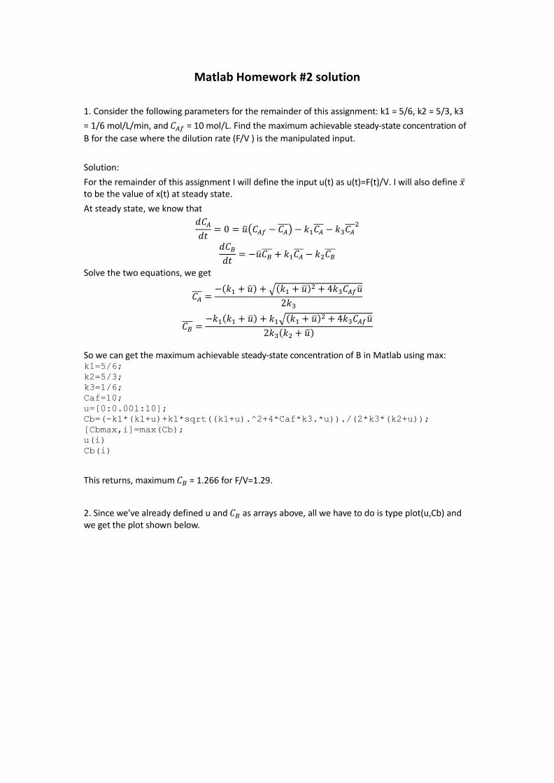
Matlab Homework #2 solution
1. Consider the following parameters for the remainder of this assignment: k1 = 5/6, k2 = 5/3, k3
= 1/6 mol/L/min, and 𝐶𝐴𝑓 = 10 mol/L. Find the maximum achievable steady-state concentration of
B for the case where the dilution rate (F/V ) is the manipulated input.
Solution:
For the remainder of this assignment I will define the input u(t) as u(t)=F(t)/V. I will also define �� to be the value of x(t) at steady state.
At steady state, we know that
𝑑𝐶𝐴
𝑑𝑡= 0 = ��(𝐶𝐴𝑓 − 𝐶𝐴
) − 𝑘1𝐶𝐴 − 𝑘3𝐶𝐴
2
𝑑𝐶𝐵
𝑑𝑡= −��𝐶𝐵
+ 𝑘1𝐶𝐴 − 𝑘2𝐶𝐵
Solve the two equations, we get
𝐶𝐴 =
−(𝑘1 + ��) + √(𝑘1 + ��)2 + 4𝑘3𝐶𝐴𝑓��
2𝑘3
𝐶𝐵 =
−𝑘1(𝑘1 + ��) + 𝑘1√(𝑘1 + ��)2 + 4𝑘3𝐶𝐴𝑓��
2𝑘3(𝑘2 + ��)
So we can get the maximum achievable steady-state concentration of B in Matlab using max:
k1=5/6; k2=5/3; k3=1/6; Caf=10; u=[0:0.001:10]; Cb=(-k1*(k1+u)+k1*sqrt((k1+u).^2+4*Caf*k3.*u))./(2*k3*(k2+u)); [Cbmax,i]=max(Cb); u(i) Cb(i)
This returns, maximum 𝐶𝐵 = 1.266 for F/V=1.29.
2. Since we've already defined u and 𝐶𝐵 as arrays above, all we have to do is type plot(u,Cb) and we get the plot shown below.

3. Build an open-loop Simulink model with the dilution rate (F/V) as the input and concentration of B (𝐶𝐵) as the output. See the figure below:
4. The maximum achievable concentration of B corresponds to a singularity, and the system is uncontrollable at this point. Instead consider both of the steady states corresponding to 𝐶𝐵 = 1.117 mol/L (F/V= 0.5714 min−1 and F/V = 2.8744 min−1 ). Use the open-loop Simulink model to find the linear state-space model for both steady-state operating points. 1) For F/V= 0.5714, 𝐶𝐴=2.9999
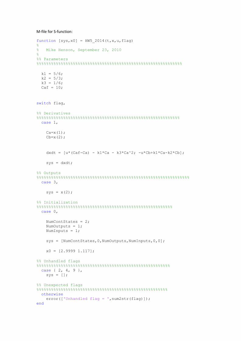
M-file for S-function:
function [sys,x0] = HW5_2014(t,x,u,flag) % % Mike Henson, September 23, 2010 % %% Parameters
%%%%%%%%%%%%%%%%%%%%%%%%%%%%%%%%%%%%%%%%%%%%%%%%%%%%%%%%%%%%
k1 = 5/6; k2 = 5/3; k3 = 1/6; Caf = 10;
switch flag,
%% Derivatives
%%%%%%%%%%%%%%%%%%%%%%%%%%%%%%%%%%%%%%%%%%%%%%%%%%%%%%%%%%% case 1,
Ca=x(1); Cb=x(2);
dxdt = [u*(Caf-Ca) - k1*Ca - k3*Ca^2; -u*Cb+k1*Ca-k2*Cb];
sys = dxdt;
%% Outputs
%%%%%%%%%%%%%%%%%%%%%%%%%%%%%%%%%%%%%%%%%%%%%%%%%%%%%%%%%%%%%%% case 3,
sys = x(2);
%% Initialization
%%%%%%%%%%%%%%%%%%%%%%%%%%%%%%%%%%%%%%%%%%%%%%%%%%%%%%%% case 0,
NumContStates = 2; NumOutputs = 1; NumInputs = 1;
sys = [NumContStates,0,NumOutputs,NumInputs,0,0];
x0 = [2.9999 1.117];
%% Unhandled flags
%%%%%%%%%%%%%%%%%%%%%%%%%%%%%%%%%%%%%%%%%%%%%%%%%%%%%%% case { 2, 4, 9 }, sys = [];
%% Unexpected flags
%%%%%%%%%%%%%%%%%%%%%%%%%%%%%%%%%%%%%%%%%%%%%%%%%%%%%% otherwise error(['Unhandled flag = ',num2str(flag)]); end
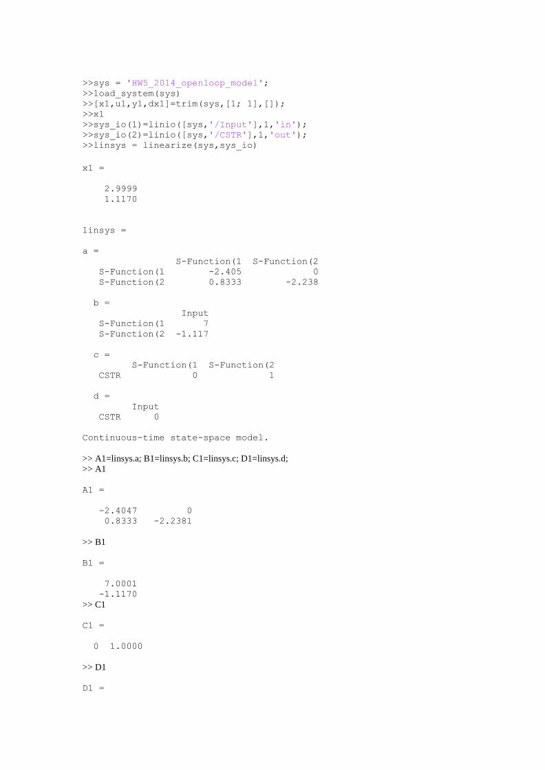
>>sys = 'HW5_2014_openloop_model'; >>load_system(sys) >>[x1,u1,y1,dx1]=trim(sys,[1; 1],[]); >>x1 >>sys_io(1)=linio([sys,'/Input'],1,'in'); >>sys_io(2)=linio([sys,'/CSTR'],1,'out'); >>linsys = linearize(sys,sys_io)
x1 =
2.9999
1.1170
linsys =
a =
S-Function(1 S-Function(2
S-Function(1 -2.405 0
S-Function(2 0.8333 -2.238
b =
Input
S-Function(1 7
S-Function(2 -1.117
c =
S-Function(1 S-Function(2
CSTR 0 1
d =
Input
CSTR 0
Continuous-time state-space model.
>> A1=linsys.a; B1=linsys.b; C1=linsys.c; D1=linsys.d;
>> A1
A1 =
-2.4047 0
0.8333 -2.2381
>> B1
B1 =
7.0001
-1.1170
>> C1
C1 =
0 1.0000
>> D1
D1 =
0
2) For F/V= 2.8714, Ca=6.0828 M-file for S-function is the same but x0=[6.0828 1.117] The linear state-space model is A2 =
-5.7353 0
0.8333 -4.5411
B2 =
3.9172
-1.1170
C2 =
0 1.0000
D2=0
5. Compute the eigenvalues of each state-space model and determine the stability of each steady state.
>> eig(A1)
ans =
-2.2381
-2.4047
>> eig(A2)
ans =
-4.5411
-5.7353
Since both of these sets of characteristic values are real and negative, both steady states are stable. We would expect a perturbation from the steady state to decay without oscillation.
6. Find the transfer function G(s)=C B (s)/D(s) corresponding to each state-space model (D ≡F/V).
One can find it easily using MATLAB
>> [num1,den1] = ss2tf(A1,B1,C1,D1); G1=tf(num1,den1)
Transfer function:
G1 =
-1.117 s + 3.147
---------------------
s^2 + 4.643 s + 5.382
>> [num2,den2] = ss2tf(A2,B2,C2,D2); G2=tf(num2,den2)

Transfer function: G2 =
-1.117 s - 3.142
---------------------
s^2 + 10.28 s + 26.04
7. Find zeroes and poles
Matlab:
>> roots(num1) ans =
2.8177
>> roots(den1) ans =
-2.4047
-2.2381
>> roots(num2)
ans =
-2.8129
>> roots(den2)
ans =
-5.7353
-4.5411
8. Use the direct substitution method and the transfer function models to analytically determine the ultimate controller gain (K cu ) for each steady state.
The poles of the closed loop transfer function are the poles of the open loop transfer function, GOL (s) = Kc Gp (s) for a proportional controller, and the roots of 1 + GOL . Since Gp (s) is stable in this problem, we only need worry about 1+GOL . Substituting s=iω and thereby forcing the poles onto the imaginary axis, we get:
For steady state 1:
1 + 𝐾𝑐𝑢
−1.117𝑖𝜔 + 3.147
(𝑖𝜔)2 + 4.643𝑖𝜔 + 5.382= 0
(4.643𝜔 − 1.117𝐾𝑐𝑢𝜔)𝑖 + (−𝜔2 + 3.147𝐾𝑐𝑢 + 5.382) = 0
𝐾𝑐𝑢 = 4.157𝐿
𝑚𝑜𝑙. 𝑚𝑖𝑛
For steady state 2:
1 + 𝐾𝑐𝑢
−1.117𝑖𝜔 − 3.147
(𝑖𝜔)2 + 10.28𝑖𝜔 + 26.05= 0
(10.28ω − 1.117𝐾cu𝜔)𝑖 + (−𝜔2 + 3.147𝐾𝑐𝑢 + 26.05) = 0
𝐾𝑐𝑢 = 9.203𝐿
𝑚𝑜𝑙. 𝑚𝑖𝑛
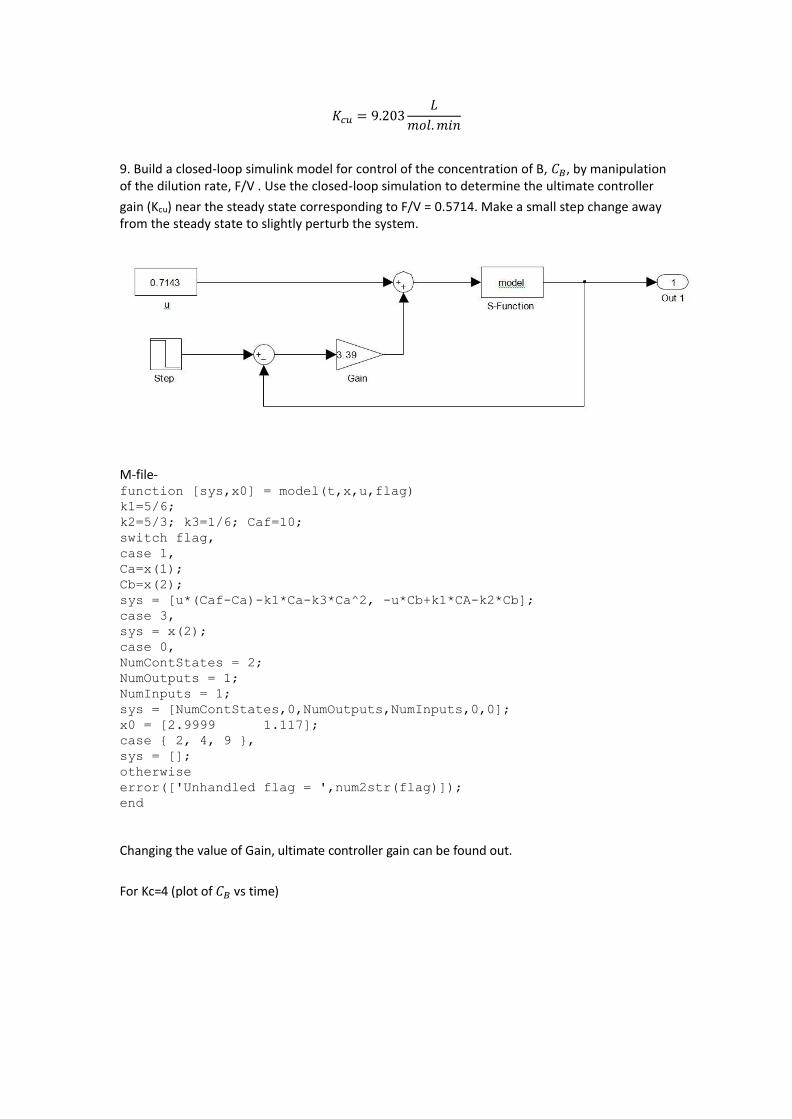
9. Build a closed-loop simulink model for control of the concentration of B, 𝐶𝐵, by manipulation of the dilution rate, F/V . Use the closed-loop simulation to determine the ultimate controller
gain (Kcu) near the steady state corresponding to F/V = 0.5714. Make a small step change away from the steady state to slightly perturb the system.
M-file- function [sys,x0] = model(t,x,u,flag)
k1=5/6;
k2=5/3; k3=1/6; Caf=10;
switch flag,
case 1,
Ca=x(1);
Cb=x(2);
sys = [u*(Caf-Ca)-k1*Ca-k3*Ca^2, -u*Cb+k1*CA-k2*Cb];
case 3,
sys = x(2);
case 0,
NumContStates = 2;
NumOutputs = 1;
NumInputs = 1;
sys = [NumContStates,0,NumOutputs,NumInputs,0,0];
x0 = [2.9999 1.117];
case { 2, 4, 9 },
sys = [];
otherwise
error(['Unhandled flag = ',num2str(flag)]);
end
Changing the value of Gain, ultimate controller gain can be found out.
For Kc=4 (plot of 𝐶𝐵 vs time)
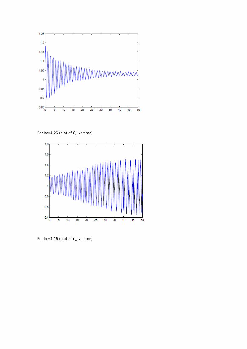
For Kc=4.25 (plot of 𝐶𝐵 vs time)
For Kc=4.16 (plot of 𝐶𝐵 vs time)
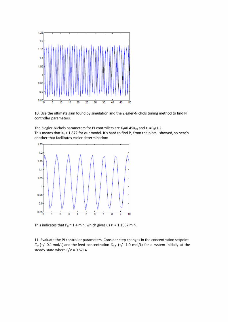
10. Use the ultimate gain found by simulation and the Ziegler-Nichols tuning method to find PI controller parameters. The Ziegler-Nichols parameters for PI controllers are Kc=0.45Kcu and τI =Pu/1.2. This means that Kc = 1.872 for our model. It's hard to find Pu from the plots I showed, so here's another that facilitates easier determination:
This indicates that Pu ~ 1.4 min, which gives us τI = 1.1667 min. 11. Evaluate the PI controller parameters. Consider step changes in the concentration setpoint 𝐶𝐵 (+/- 0.1 mol/L) and the feed concentration 𝐶𝐴𝑓 (+/- 1.0 mol/L) for a system initially at the
steady-state where F/V = 0.5714.
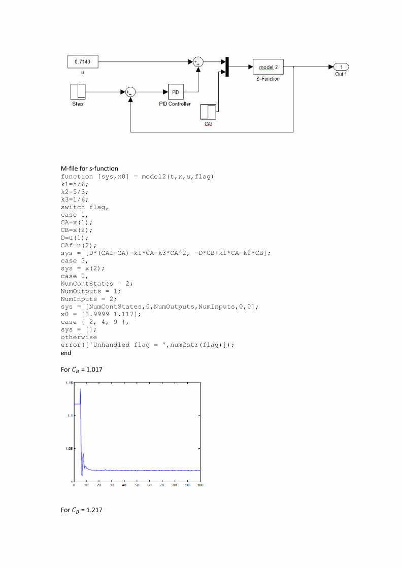
M-file for s-function function [sys,x0] = model2(t,x,u,flag)
k1=5/6;
k2=5/3;
k3=1/6;
switch flag,
case 1,
CA=x(1);
CB=x(2);
D=u(1);
CAf=u(2);
sys = [D*(CAf-CA)-k1*CA-k3*CA^2, -D*CB+k1*CA-k2*CB];
case 3,
sys = x(2);
case 0,
NumContStates = 2;
NumOutputs = 1;
NumInputs = 2;
sys = [NumContStates,0,NumOutputs,NumInputs,0,0];
x0 = [2.9999 1.117];
case { 2, 4, 9 },
sys = [];
otherwise
error(['Unhandled flag = ',num2str(flag)]);
end
For 𝐶𝐵 = 1.017
For 𝐶𝐵 = 1.217
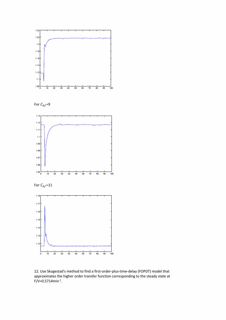
For 𝐶𝐴𝑓=9
For 𝐶𝐴𝑓=11
12. Use Skogestad's method to find a first-order-plus-time-delay (FOPDT) model that approximates the higher order transfer function corresponding to the steady state at F/V=0.5714min-1.
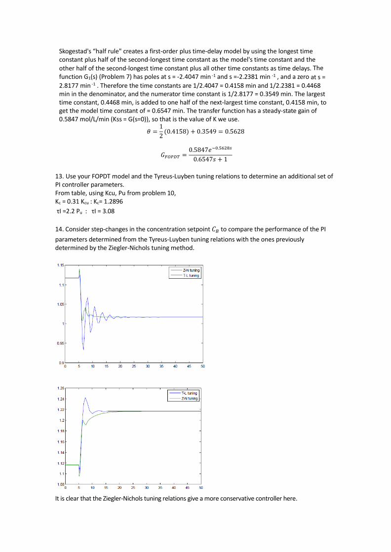
Skogestad's “half rule" creates a first-order plus time-delay model by using the longest time constant plus half of the second-longest time constant as the model's time constant and the
other half of the second-longest time constant plus all other time constants as time delays. The
function G1(s) (Problem 7) has poles at s = -2.4047 min -1 and s =-2.2381 min -1 , and a zero at s = 2.8177 min -1 . Therefore the time constants are 1/2.4047 = 0.4158 min and 1/2.2381 = 0.4468 min in the denominator, and the numerator time constant is 1/2.8177 = 0.3549 min. The largest time constant, 0.4468 min, is added to one half of the next-largest time constant, 0.4158 min, to get the model time constant of = 0.6547 min. The transfer function has a steady-state gain of 0.5847 mol/L/min (Kss = G(s=0)), so that is the value of K we use.
𝜃 =1
2(0.4158) + 0.3549 = 0.5628
𝐺𝐹𝑂𝑃𝐷𝑇 =0.5847𝑒−0.5628𝑠
0.6547𝑠 + 1
13. Use your FOPDT model and the Tyreus-Luyben tuning relations to determine an additional set of PI controller parameters. From table, using Kcu, Pu from problem 10, Kc = 0.31 Kcu : Kc= 1.2896
τI =2.2 Pu : τI = 3.08
14. Consider step-changes in the concentration setpoint 𝐶𝐵 to compare the performance of the PI
parameters determined from the Tyreus-Luyben tuning relations with the ones previously determined by the Ziegler-Nichols tuning method.
It is clear that the Ziegler-Nichols tuning relations give a more conservative controller here.