Embed Size (px)
Citation preview
TYPES OF IIR FILTERS
1/19
• Bu#erworth -‐ Maximally flat magnitude in the passband
• Chebyshev type I -‐ Equiripple in the passband
• Chebyshev type II -‐ Equiripple in the stopband
• Ellip5c -‐ Equiripple in passband and stopband
• Bessel -‐ Maximally flat group delay
ECE580 – Fall 2010
CONTINUOUS-‐TIME FILTERS
2/19
• MATLAB command
-‐ buPord, buPer (BUTTERWORTH)
-‐ cheb1ord, cheb1 (CHEBYSHEV TYPE I) -‐ cheb2ord, cheb2 (CHEBYSHEV TYPE II) -‐ ellipord, ellip (ELLIPTIC)
-‐ besself (BESSEL)
• Use with ‘s’ op[on for con[nuous [me
• Frequency are in rad/s • APenua[on and ripple values are in dB
ECE580 – Fall 2010
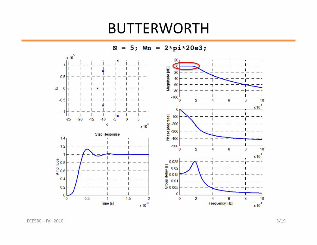
BUTTERWORTH
3/19 ECE580 – Fall 2010
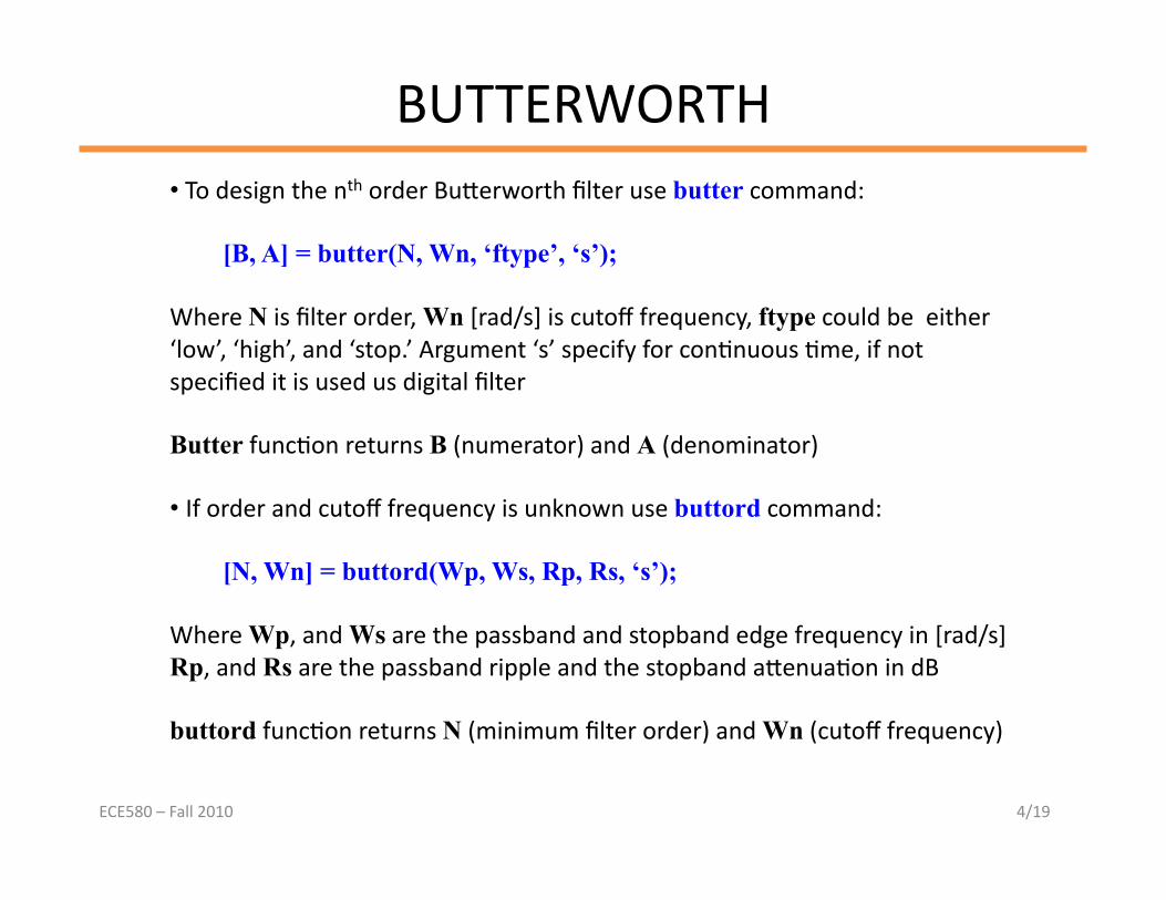
BUTTERWORTH
4/19
• To design the nth order BuPerworth filter use butter command:
[B, A] = butter(N, Wn, ‘ftype’, ‘s’);
Where N is filter order, Wn [rad/s] is cutoff frequency, ftype could be either ‘low’, ‘high’, and ‘stop.’ Argument ‘s’ specify for con[nuous [me, if not specified it is used us digital filter
Butter func[on returns B (numerator) and A (denominator)
• If order and cutoff frequency is unknown use buttord command:
[N, Wn] = buttord(Wp, Ws, Rp, Rs, ‘s’);
Where Wp, and Ws are the passband and stopband edge frequency in [rad/s] Rp, and Rs are the passband ripple and the stopband aPenua[on in dB
buttord func[on returns N (minimum filter order) and Wn (cutoff frequency)
ECE580 – Fall 2010
CHEBYSHEV TYPE I
5/19 ECE580 – Fall 2010
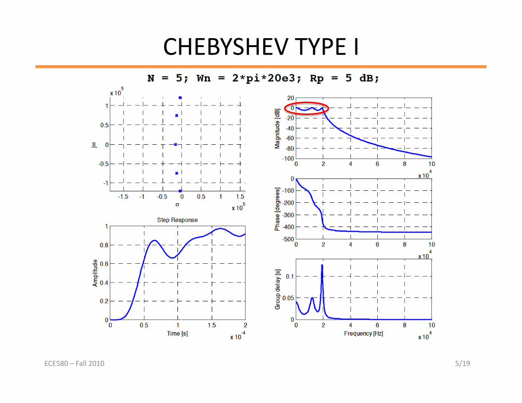
CHEBYSHEV TYPE I
6/19
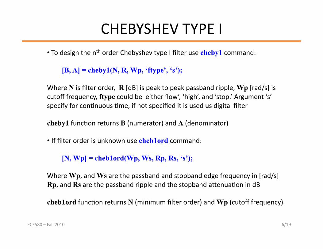
• To design the nth order Chebyshev type I filter use cheby1 command:
[B, A] = cheby1(N, R, Wp, ‘ftype’, ‘s’);
Where N is filter order, R [dB] is peak to peak passband ripple, Wp [rad/s] is cutoff frequency, ftype could be either ‘low’, ‘high’, and ‘stop.’ Argument ‘s’ specify for con[nuous [me, if not specified it is used us digital filter
cheby1 func[on returns B (numerator) and A (denominator)
• If filter order is unknown use cheb1ord command:
[N, Wp] = cheb1ord(Wp, Ws, Rp, Rs, ‘s’);
Where Wp, and Ws are the passband and stopband edge frequency in [rad/s] Rp, and Rs are the passband ripple and the stopband aPenua[on in dB
cheb1ord func[on returns N (minimum filter order) and Wp (cutoff frequency)
ECE580 – Fall 2010
CHEBYSHEV TYPE II
7/19 ECE580 – Fall 2010
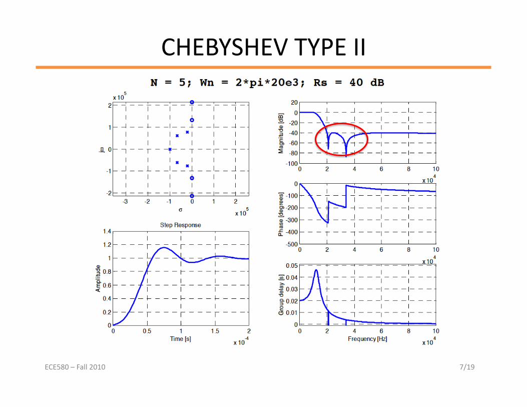
CHEBYSHEV TYPE II
8/19
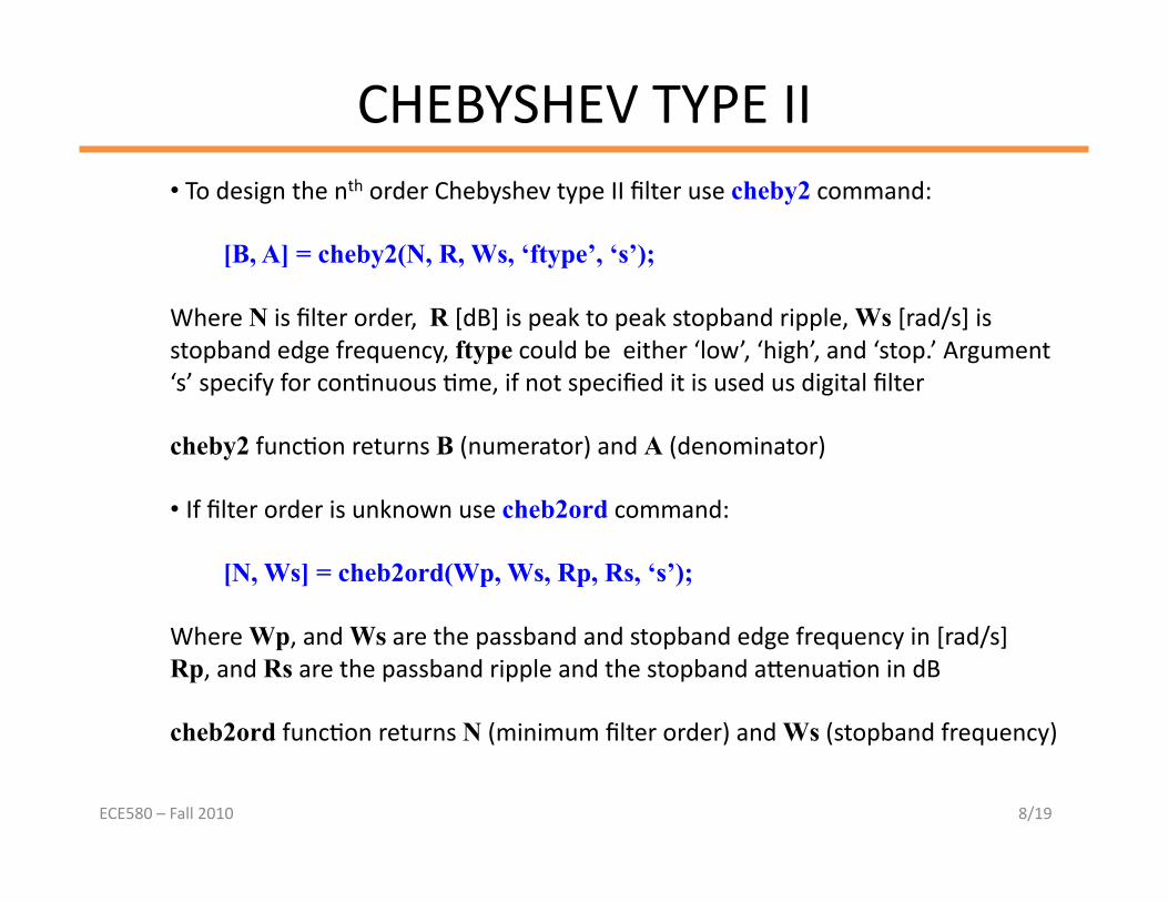
• To design the nth order Chebyshev type II filter use cheby2 command:
[B, A] = cheby2(N, R, Ws, ‘ftype’, ‘s’);
Where N is filter order, R [dB] is peak to peak stopband ripple, Ws [rad/s] is stopband edge frequency, ftype could be either ‘low’, ‘high’, and ‘stop.’ Argument ‘s’ specify for con[nuous [me, if not specified it is used us digital filter
cheby2 func[on returns B (numerator) and A (denominator)
• If filter order is unknown use cheb2ord command:
[N, Ws] = cheb2ord(Wp, Ws, Rp, Rs, ‘s’);
Where Wp, and Ws are the passband and stopband edge frequency in [rad/s] Rp, and Rs are the passband ripple and the stopband aPenua[on in dB
cheb2ord func[on returns N (minimum filter order) and Ws (stopband frequency)
ECE580 – Fall 2010
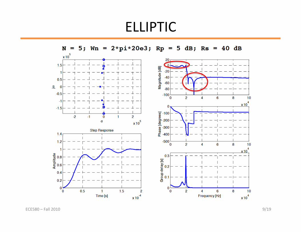
ELLIPTIC
9/19 ECE580 – Fall 2010

ELLIPTIC
10/19
• To design the nth order ellip[c filter use ellip command:
[B, A] = ellip(N, Rp, Rs, Wp, ‘ftype’, ‘s’);
Where N is filter order, Rp and Rs [dB] is peak to peak passband and stopband ripple, Wp [rad/s] is stopband edge frequency, ftype could be either ‘low’, ‘high’, and ‘stop.’ Argument ‘s’ specify for con[nuous [me, if not specified it is used us digital filter
ellip func[on returns B (numerator) and A (denominator)
• If filter order is unknown use ellipord command:
[N, Wp] = ellipord(Wp, Ws, Rp, Rs, ‘s’);
Where Wp, and Ws are the passband and stopband edge frequency in [rad/s] Rp, and Rs are the passband ripple and the stopband aPenua[on in dB
ellipord func[on returns N (minimum filter order) and Wp (passband frequency)
ECE580 – Fall 2010
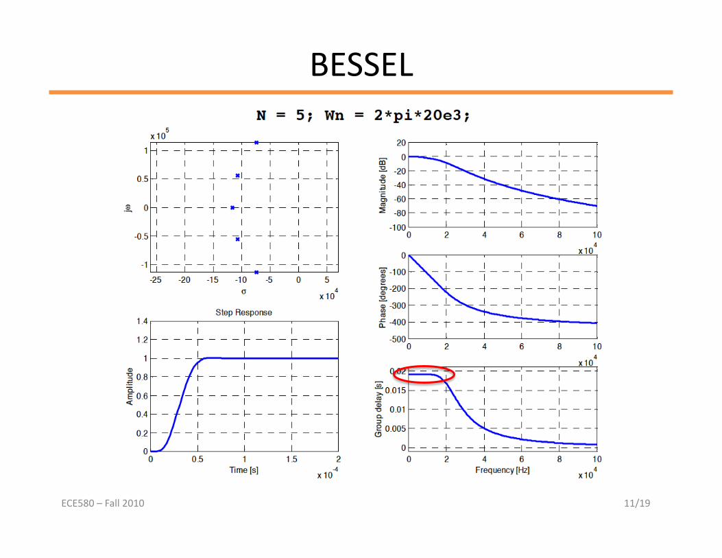
BESSEL
11/19 ECE580 – Fall 2010
BESSEL
12/19
• To design the nth order bessel filter use besself command:
[B, A] = besself(N, Wo);
Where N is filter order, Wo [rad/s] is the frequency up to which the group delay is approximately constant
besself func[on returns B (numerator) and A (denominator)
• besself func[on can only design analog filters
ECE580 – Fall 2010
DISCRETE-‐TIME FILTERS
13/19
• Use same command without ‘s’ op[on
• Frequency are normalized to Fs/2
-‐
ECE580 – Fall 2010
€
Wn =1⇒ f = Fs /2

Z-‐PLANE REPRESENTATION
14/19 ECE580 – Fall 2010
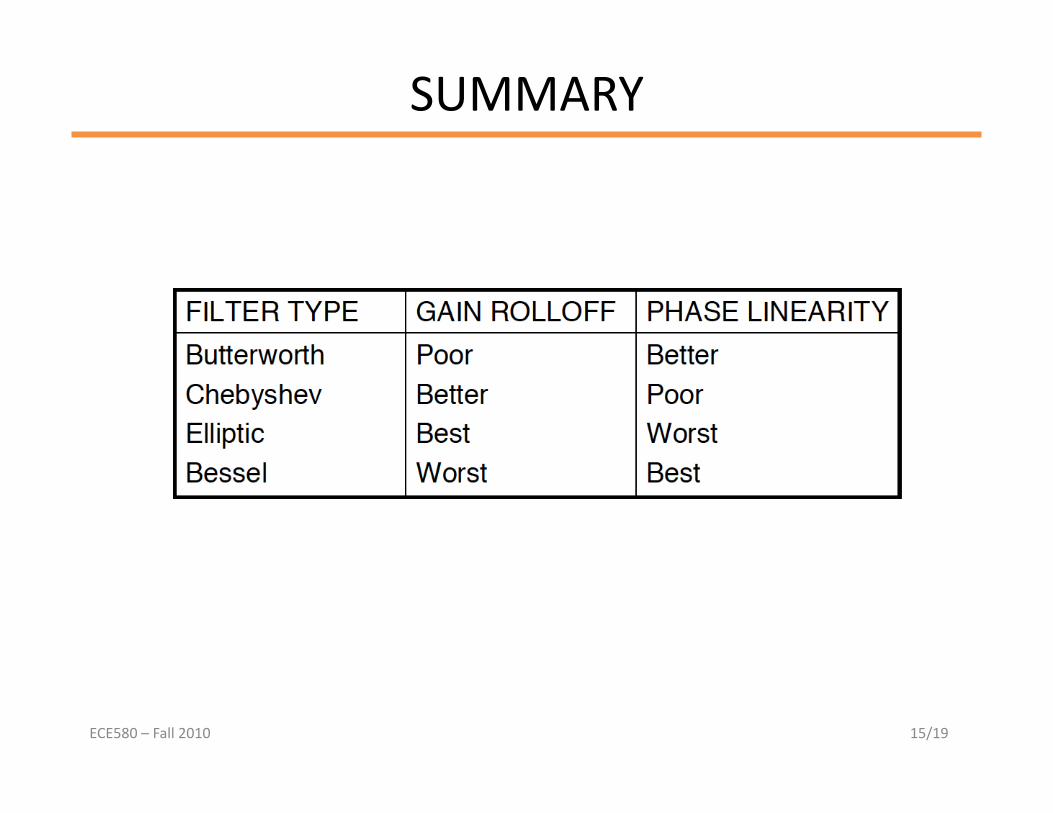
SUMMARY
15/19 ECE580 – Fall 2010
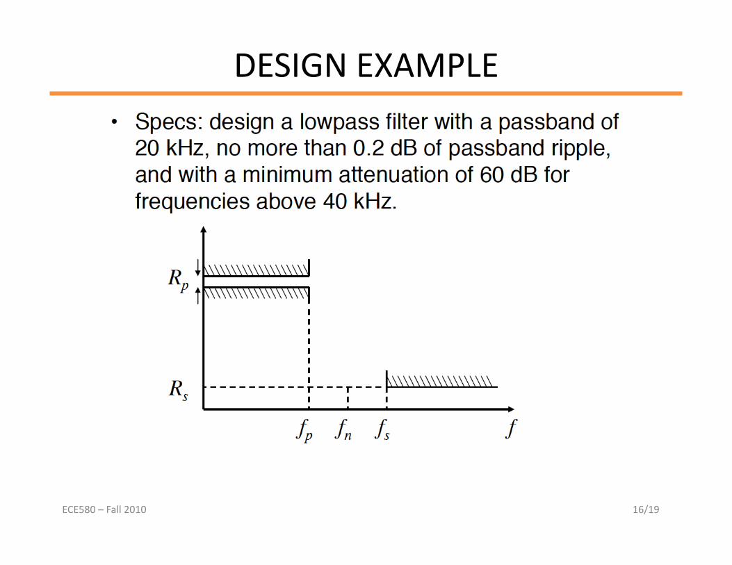
DESIGN EXAMPLE
16/19 ECE580 – Fall 2010
DESIGN EXAMPLE
17/19 ECE580 – Fall 2010
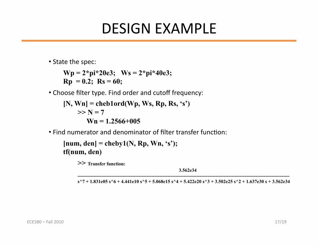
• State the spec: Wp = 2*pi*20e3; Ws = 2*pi*40e3; Rp = 0.2; Rs = 60;
• Choose filter type. Find order and cutoff frequency: [N, Wn] = cheb1ord(Wp, Ws, Rp, Rs, ‘s’) >> N = 7 Wn = 1.2566+005
• Find numerator and denominator of filter transfer func[on:
[num, den] = cheby1(N, Rp, Wn, ‘s’); tf(num, den) >> Transfer function:
3.562e34 ------------------------------------------------------------------------------------------------------------------------------------s^7 + 1.831e05 s^6 + 4.441e10 s^5 + 5.068e15 s^4 + 5.422e20 s^3 + 3.502e25 s^2 + 1.637e30 s + 3.562e34
DESIGN EXAMPLE
18/19 ECE580 – Fall 2010
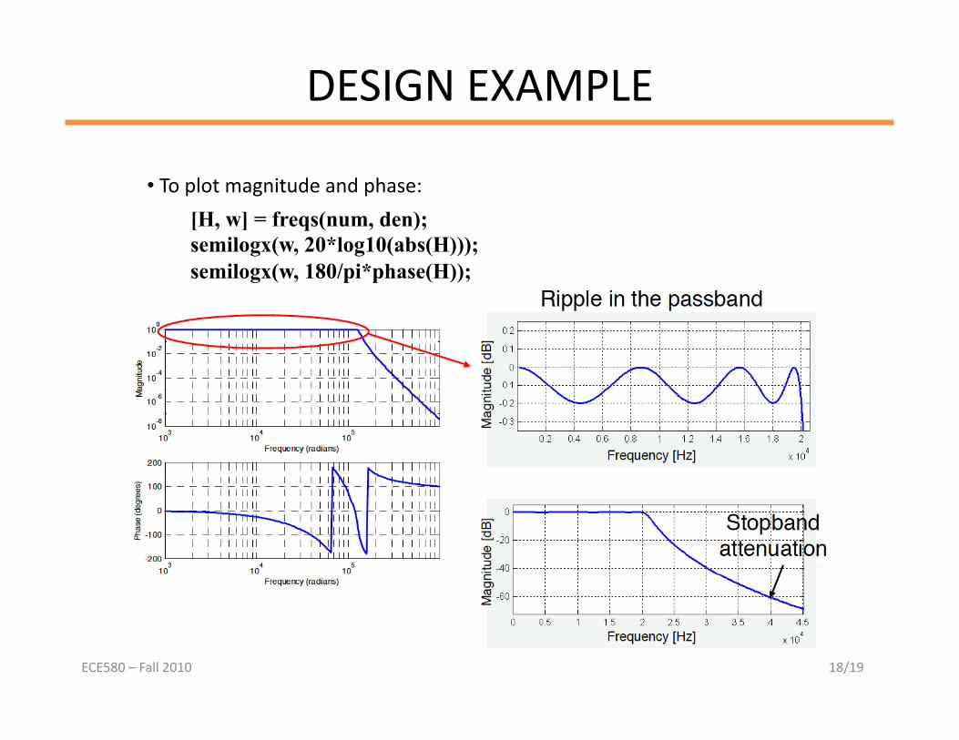
• To plot magnitude and phase:
[H, w] = freqs(num, den); semilogx(w, 20*log10(abs(H))); semilogx(w, 180/pi*phase(H));
DESIGN EXAMPLE
19/19 ECE580 – Fall 2010
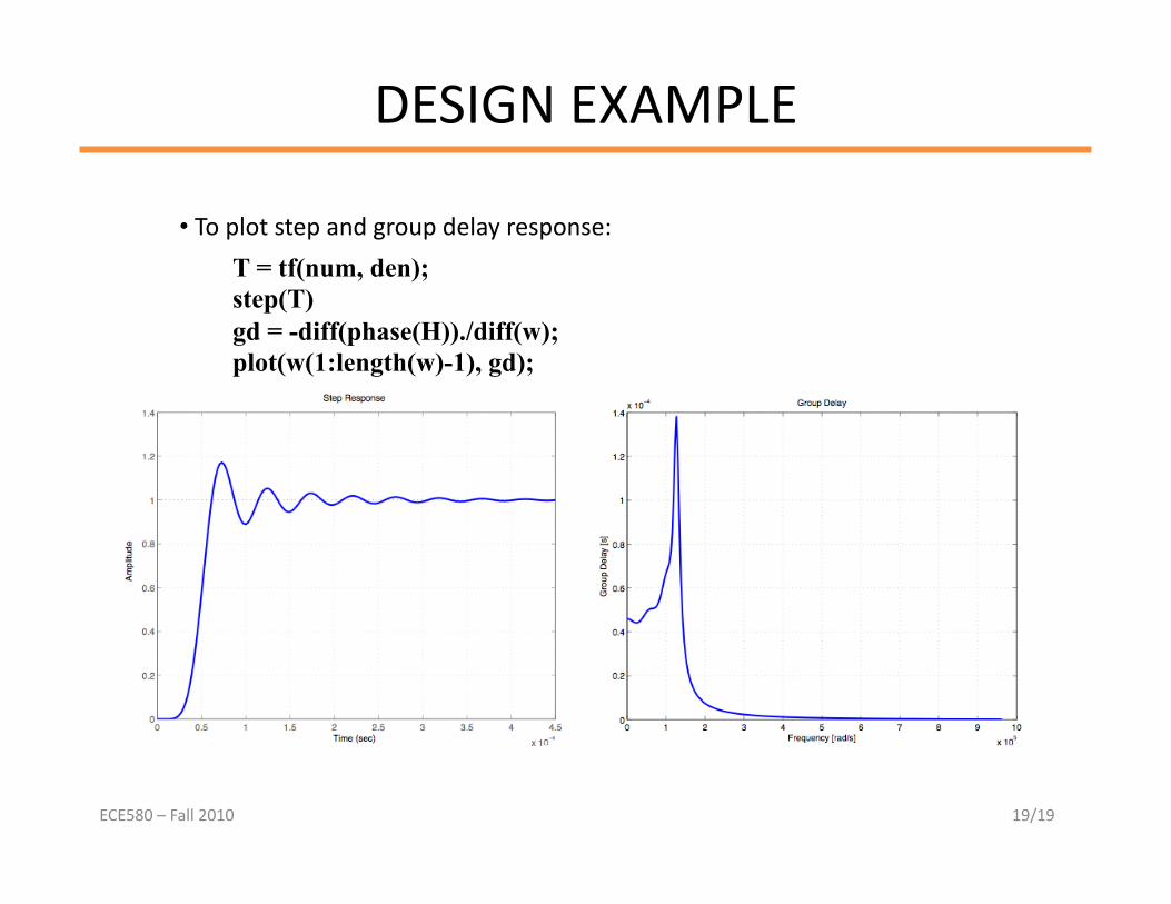
• To plot step and group delay response: T = tf(num, den); step(T) gd = -diff(phase(H))./diff(w); plot(w(1:length(w)-1), gd);