AC 2008-844: MATLAB/SIMULINK LAB EXERCISES DESIGNED FORTEACHING DIGITAL SIGNAL PROCESSING APPLICATIONS

Kathleen Ossman, University of CincinnatiDr. Kathleen Ossman is an associate professor in the Electrical and Computer EngineeringTechnology Department at the University of Cincinnati. She earned a BSEE and MSEE fromGeorgia Tech in 1982 and a Ph.D. from the University of Florida in 1986. Her interests includedigital signal processing and feedback control.

© American Society for Engineering Education, 2008

Page 13.872.1

MATLAB/Simulink Lab Exercises Designed for

Teaching Digital Signal Processing Applications

Abstract

This paper describes a collection of MATLAB/Simulink exercises designed for a sequence of

digital signal processing (DSP) lab courses that run concurrently with lecture courses in DSP.

The labs are designed to introduce electrical and computer engineering technology students to

some of the practical considerations and applications of digital signal processing. The labs

enhance and expand upon the theory discussed in lecture; moving students from mathematical

gswcvkqpu"vq"Ðjcpfu"qpÑ"gzrgtkgpeg"cpf"gzrgtkogpvcvkqp0

Introduction

Digital signal processing theory involves fairly sophisticated mathematics including difference

equations, Z-Transforms, fast Fourier Transforms, and stochastic analysis. For electrical and

computer engineering technology students, this level of mathematics can be daunting. Providing

applications and exercises to illustrate the theory is therefore essential in teaching DSP to

engineering technology students.

Hqwt"ncd"gzgtekugu"yknn"dg"fguetkdgf"kp"vjku"rcrgt0"Kp"vjg"ÐGhhgev"qh"Hknvgt"Eoefficient Wordlengthon Uvcdknkv{"cpf"RgthqtocpegÑ"ncd."uvwfgpvu"fgukip"KKT"hknvgtu"wukpi"vjg"Hknvgt"Fgukip"cpf"Analysis Tool (FDAT) in MATLAB. Students then quantize the filter coefficients to various bit

sizes and explore the effect on filter performance and stability. "Vjg"ÐKocig"Rtqeguukpi"wukpi"Digital"HknvgtuÑ"ncd"knnwuvtcvgu"vjg"ghhgev"qh"uoqqvjkpi"cpf"ujctrgpkpi"hknvgtu"qp"kocigu"cpf"cnuqgzrnqtgu"vjg"LRGI"hqtocv0""ÐTcfct"Tcpig"Rtqeguukpi"wukpi"Ejktr"UkipcnuÑ"kpvtqfwegu"uvwfgpvu"vq"chirp signals and the design of matched filters for determining target range and velocity. Finally,

vjg"ÐHcuv"Eqpxqnwvkqp"wukpi"Qxgtncr-Cff"RtqeguukpiÑ"tgswktgs students to write an m-file for areal-time filtering algorithm using an FIR filter designed in MATLAB and an arbitrary input

signal. These lab exercises are very effective both in illustrating digital signal processing theory

and getting students excited about DSP applications.

Effect of Filter Coefficient Wordlength on Stability and Performance

Digital filters are sensitive to wordlength effects; that is, seemingly small amounts of rounding of

the filter coefficients can lead to significant degradation in the filter performance. For infinite

impulse response (IIR) filters, rounding of the coefficients can result in an unstable filter. The

sensitivity to wordlength effects can be reduced for IIR filters by implementing the filter in 2nd

order sections (biquads) instead of in a single Nthorder block. Students explore the wordlength

effect for IIR filters both in single block and biquad realizations using MATLAB. After

simulating the effects, students download rounded coefficients onto Texas InstrumepvuÓTMS320C6711 DSKs and verify that experimental results correlate with simulation results.

Page 13.872.2

The objectives of this lab exercise are to:

1. Become proficient at using the Filter Design and Analysis Tool to design IIR filters.

2. Understand the format used when exporting filter coefficients to MATLAB for both a full

realization and a biquad realization.

3. Investigate the effect of coefficient wordlength on IIR filter stability and performance for

both a full realization and a biquad realization.

A summary of procedure for this lab exercise is:

1. Design an IIR filter (single block realization) of your choice using the Filter Design and

Analysis Tool in MATLAB.

2. Export the filter coefficient to the MATLAB workspace.

3. Determine the minimum number of bits for the coefficients to ensure stability of the

filter.

4. Plot the frequency response (magnitude) using the minimum number of bits.

5. Determine the number of bits required to give good filter performance (i.e. meet original

specifications.

6. Return to the Filter Design and Analysis Tool and realize the same IIR filter using 2nd

order sections.

7. Determine the minimum number of bits for stability and plot the frequency response

(magnitude) for this minimum number of bits.

8. Determine the number of bits required to give good filter performance for the biquad

realization.

A specific example is used in this paper to illustrate the outcomes of the exercise. Using the

Filter Design and Analysis Tool, an IIR elliptic band-pass filter is designed to meet the following

specifications:

Passband: 8 Î 12 KHz Maximum Passband Ripple: 0.1 dB

Stopband: < 7 KHz and > 13 KHz

Minimum Stopband Attenuation: 30 dB

Sampling Frequency: 48 KHz

The filter turns out to be 10thorder. The minimum number of bits required for stability (in a

single block) is determined using the m-file shown in Figure 1.

Students simply vary the number of bits, B, and look at the resulting filter poles. The filter

becomes unstable when one or more filter poles has a magnitude greater than or equal to 1.0.

For this particular example, the minimum number of bits required for filter stability is 9. The m-

file in Figure 1 is also used to plot the filter frequency response (magnitude) for a specified

number of bits, B. Figure 2 illustrates the filter performance using the minimum number of bits

(poor but stable) and the filter performance using more bits (16) in order to meet specifications. Page 13.872.3

Figure 1: m-file for Stability and Performance - Single Block Realization

Figure 2: IIR Filter Performance for Single Block Realization

Page 13.872.4

Student then return to the Filter Design and Analysis Tool and convert the IIR filter to 2ndorder

sections. Since the filter in this example is 10thorder, the 2

ndorder realization will consist of five

biquads. The filter is then exported to MATLAB as an SOS (Second Order Section) matrix and

a G (Gain) vector. The m-file shown in Figure 3 is used to evaluate stability of each second

order section for B bits (varied by students for their filter) and to plot the frequency response

(magnitude) for a specified number of bits, B.

Figure 3: m-file for Stability and Performance Î Biquad Realization

Results for the example filter in this paper are illustrated in Figure 4. The minimum number of

bits for stability is reduced from 9 bits to 5 bits if 2ndorder sections are used for filter

implementation. Good filter performance can be achieved with only 9 bits for a 2ndorder

implementation while 16 bits are required for a single block realization.

It is important to allow each student to select their own filter for this analysis. Students will then

see a lot of variance in results among the class depending on how stringent the original filter

requirements are. That is, low pass filters with fairly wide transition bands will not require

nearly as many bits for good performance as high Q-factor band-pass filters will.

Following simulation, students implement the IIR filters for a couple of choices of bits (good and

rqqt+"qp"Vgzcu"KpuvtwogpvuÓ"VOU542E8933"FUMu to verify the simulation resultsexperimentally.

Page 13.872.5

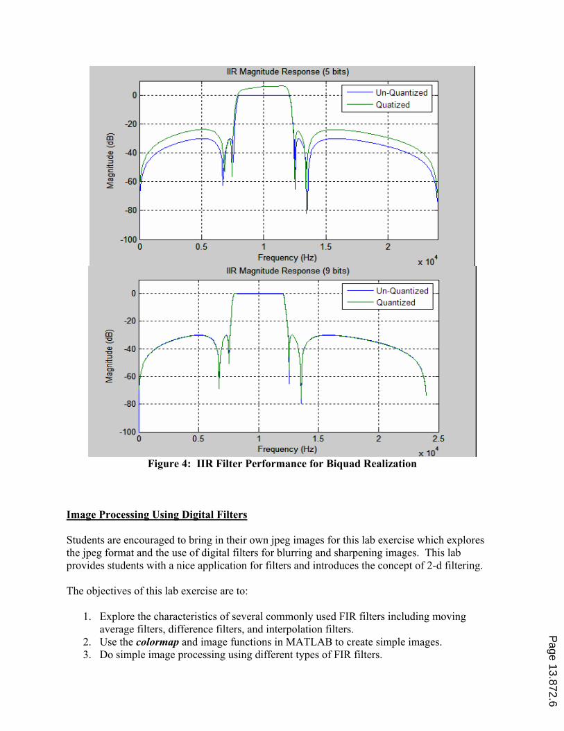
Figure 4: IIR Filter Performance for Biquad Realization

Image Processing Using Digital Filters

Students are encouraged to bring in their own jpeg images for this lab exercise which explores

the jpeg format and the use of digital filters for blurring and sharpening images. This lab

provides students with a nice application for filters and introduces the concept of 2-d filtering.

The objectives of this lab exercise are to:

1. Explore the characteristics of several commonly used FIR filters including moving

average filters, difference filters, and interpolation filters.

2. Use the colormap and image functions in MATLAB to create simple images.

3. Do simple image processing using different types of FIR filters.

Page 13.872.6

Gaussian Filters for Smoothing

Gaussian Filters are commonly used in image processing software to blur or soften an image.

Images are blurred by creating a set of new pixels where each new pixel is a function of the

original pixel and some of the surrounding pixels. A very simple smoothing matrix is given by:

] _3/13/13/1

3/1

3/1

3/1

111

111

111

9

1‚

ÙÙÙ

Ú

×

ÈÈÈ

É

Ç?

ÙÙÙ

Ú

×

ÈÈÈ

É

Ç

This matrix can be used to create a new smoothed image by simply averaging the original pixel

(center of matrix) with the eight pixels surrounding the original pixel. This averaging function is

applied to the entire original image Filtering is accomplished in MATLAB by using the

function conv2 to convolve a 3-point moving average filter with both the rows and the columns

of the original image.

The simple smoothing matrix described above applies equal weight to the original pixel and all

the surrounding pixels. A Gaussian filter puts more weight on the original pixel and smaller

weighting on surrounding pixels. The weightings are determined by a Gaussian function

(perhaps the term bell curve is more familiar). An example of a smoothing matrix using a

Gaussian function is:

0.0278 0.1111 0.1667 0.1111 0.0278 1/16

0.1111 0.4444 0.6667 0.4444 0.1111 4/162

16

6ÕÖÔ

ÄÅÃ

0.1667 0.6667 1.0000 0.6667 0.1667 = 6/16 ズ" ÙÚ×

ÈÉÇ

16

1

16

4

16

6

16

4

16

1

0.1111 0.4444 0.6667 0.4444 0.1111 4/16

0.0278 0.1111 0.1667 0.1111 0.0278 1/16

The original pixel (in center) is weighted the highest while the surrounding pixels receive smaller

weightings. The pixels furthest from the center (original) are weighted the least. Additional

uniform scaling can be added to utilize the full scale available for the image. What is the

advantage of using Gaussian weighting rather than straight averaging on the pixels? Gaussian

filters provide gentler smoothing and preserve the edges in an image better than similar size

mean (averaging) filters.

Students import jpeg images into MATLAB using imread then convert the image to a black and

white image using Y = 0.299RED + 0.587GREEN + 0.114BLUE. Filtering is accomplished in

MATLAB by first creating a Gaussian filter using the function firgauss then convolving this

filter with both the rows and columns of the original image using the two dimensional

convolution function conv2.

Page 13.872.7

Sample results are shown in Figure 5. Notice that the original image appears a bit grainy,

rctvkewnctn{"ctqwpf"vjg"pqug"cpf"vjg"yjkvg"hwt"qp"vjg"fqiÓu"ejguv0""Vjg"kocig"ku"hktuv smoothedusing the 5x5 Gaussian matrix described earlier in this paper. The result is shown in the top right

window of Figure 5. The image is noticeably softened; graininess is reduced but not eliminated.

Next the image is smoothed using a 29x29 Gaussian matrix created in MATLAB using

firgauss(4,8). The resulting image, shown in the bottom left window of Figure 5, is considerably

softened eliminating the graininess in the original image but preserving the edge detail. For

comparison purposes, a similar sized (28x28) mean (averaging) filter is applied to the original

image. The application of an averaging filter to the image results in the loss of edge detail and a

blurrier image.

Figure 5: Smoothing Images through Digital Filtering

Page 13.872.8

Difference Filters for Sharpening Images

A simple filter for sharpening images by enhancing edges is given by:

ÙÙÙ

Ú

×

ÈÈÈ

É

Ç

////////

?8/18/18/1

8/18/1

8/18/18/1

CE

Students again import jpeg images using imread, convert to a black and white image (Y =

0.299RED + 0.587GREEN + 0.114BLUE), and then filter their images using conv2. Varying

the center value, C, in the matrix E affects the degree of sharpening. An example of results is

shown in Figure 6. Choosing C = 1 produces an embossed image with edges showing up white.

Higher values of C enhance the edges in the image.

Figure 6: Sharpening Images using Digital Filtering

Page 13.872.9

Radar Range Processing Using Chirp Signals

In radar range processing, a chirp signal is transmitted. The signal bounces off a target and

returns to the receiver. The time required for the echo signal to arrive at the receiver determines

the range to the target. Since radio waves travel at approximately the speed of light, the equation

to determine range is given by:

R = ½ [cTd]

R = target range in meters

c = 3*108m/s

Td = time delay required for pulse to return in seconds

The objectives of this lab exercise are to:

1. Investigate properties of chirp signals both in the time and frequency domain.

2. Design a matched filter capable of detecting a chirp signal buried in noise.

3. Use SIMULINK to simulate a radar detector that computes the range to a target based on

an echo return chirp signal buried in noise.

An LFM Chirp signal is a constant amplitude signal with a frequency which varies linearly with

time. Students experiment with the parameters of a chirp signal (over-sampling rate, p and pulse

bandwidth product, TW) using the m-file mychirp shown in Figure 6. This m-file calls the

chirp m-file included with MATLAB then adds some useful plots.

Figure 6: m-file for mychirp

Page 13.872.10

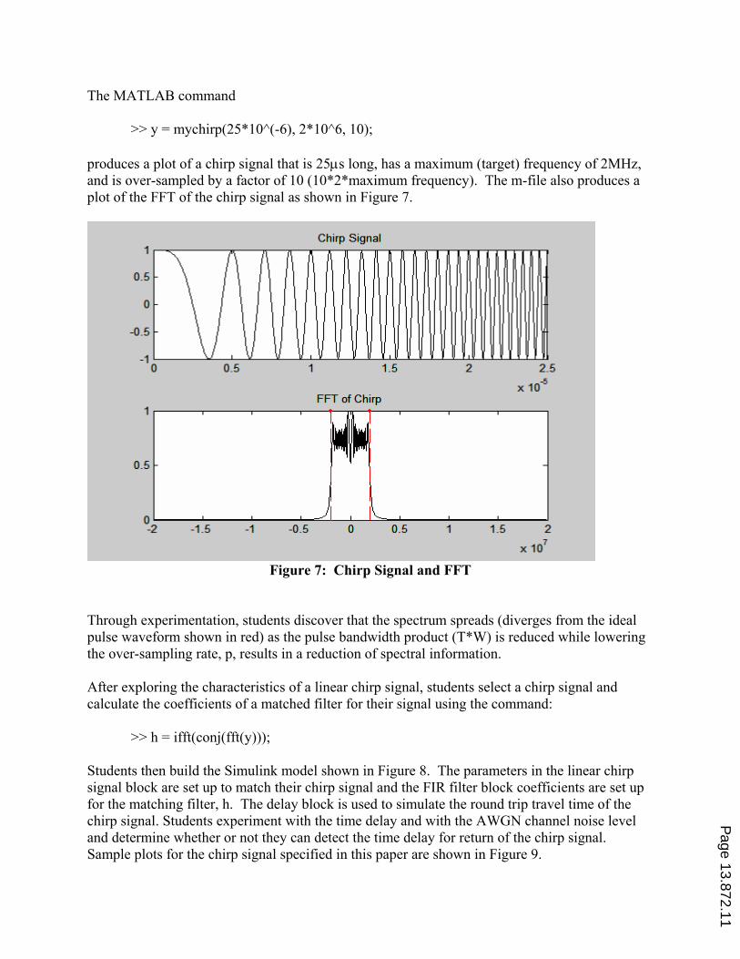
The MATLAB command

>> y = mychirp(25*10^(-6), 2*10^6, 10);

produces a plot of a chirp signal that is 25os long, has a maximum (target) frequency of 2MHz,and is over-sampled by a factor of 10 (10*2*maximum frequency). The m-file also produces a

plot of the FFT of the chirp signal as shown in Figure 7.

Figure 7: Chirp Signal and FFT

Through experimentation, students discover that the spectrum spreads (diverges from the ideal

pulse waveform shown in red) as the pulse bandwidth product (T*W) is reduced while lowering

the over-sampling rate, p, results in a reduction of spectral information.

After exploring the characteristics of a linear chirp signal, students select a chirp signal and

calculate the coefficients of a matched filter for their signal using the command:

>> h = ifft(conj(fft(y)));

Students then build the Simulink model shown in Figure 8. The parameters in the linear chirp

signal block are set up to match their chirp signal and the FIR filter block coefficients are set up

for the matching filter, h. The delay block is used to simulate the round trip travel time of the

chirp signal. Students experiment with the time delay and with the AWGN channel noise level

and determine whether or not they can detect the time delay for return of the chirp signal.

Sample plots for the chirp signal specified in this paper are shown in Figure 9.

Page 13.872.11

Figure 8: SIMULINK Model for Radar Range Processing

Figure 9: Signals from Simulink Model

Page 13.872.12

The output of the matched filter shows a distinct spike at 30 os implying that the time delay is5os (time that spike occurs Î period of chirp signal). Since the sampling rate was 40MHz andthe delay block was set to 200, the actual simulation delay is indeed 5 os (200/40M). Asstudents experiment with raising the noise level (reducing SNR in the AWGN block), they

discover a point at which the output of the matched filter does not produce the distinctive spike

required to calculate the round trip travel time of the chirp signal.

Fast Convolution Using Overlap-Add Processing

Overlap-add is an efficient algorithm for performing real-time convolution calculations. The

algorithm is explained in lecture with several accompanying numerical examples.

The objectives of the lab exercise are to:

1. Write an m-file implementing the overlap add algorithm for fast convolution. Input

parameters to the file should be FIR filter coefficients and an input signal. The file

should produce the filter output signal.

2. Verify the m-file works.

This lab exercise provides a good learning opportunity for the students. It requires an ability to

manipulate data and execute a variety of MATLAB statements. It also requires an in-depth

understanding of how the overlap-add algorithm works. This is the lab that students typically

identify as the most challenging for them.

Student Learning

Digital signal processing theory can be difficult for engineering technology students to grasp, but

it is essential that students understand principles of sampling, aliasing, filter design, etc. before

moving on to hardware-based design projects. Hands on experimentation using

MATLAB/Simulink enables them to visualize the concepts without becoming lost in the

mathematics or in hardware related issues. Including practical applications with music, sound, or

pictures definitely sparks interest.

In the wordlength effects lab, students are often surprised by the number of bits required for a

stable filter and the effect that just a little bit of rounding can actually have on the filter

performance. Because students each design and test their own filter, we end up with a large

variety of filter types and orders so there is a lot of variation in how many bits are needed for

good performance among the student in the lab. In their technical conclusion, students often

comment on these differences.

In the image processing lab, most students comment that they have used photo enhancement

software to blur or sharpen images but had no idea how these tools actually worked until they

tried the 2-d filtering in MATLAB. A moving average filter means a lot more to students after

they have seen its effect on an image. Page 13.872.13

The fast convolution lab has been a really nice addition for my students. As an instructor, I am

continually supplying MATLAB code and m-files to students in my examples and hand-outs.

Many textbooks also provide customized m-files for various applications. While these

customized m-files and codes are very convenient, they can also be detrimental in that they do

not force students to write their own code. The first time I ran this lab exercise, I was shocked

d{"o{"uvwfgpvÓu"kpcdknkv{"vq"ytkvg"vjgkt"qyp"o-files. During the lab, many students reallycomplained about how difficult this exercise was. However, in their technical conclusions, most

students commented that this was one of the most useful labs for them because they were

actually required to write their own code and as a result they felt that their MATLAB skill set

was significantly improved.

As far as test performance goes, I have not seen any diffgtgpeg"kp"uvwfgpvuÓ"rgthqtocpeg"qp"arithmetic problems with the addition of these labs. However, I have seen a significant

improvement in their ability to answer essay type questions that test their understanding of

various digital signal processing concepts.

Conclusion

Four lab exercises are presented in this paper to illustrate important digital signal processing

concepts and applications. The lab exercises are based in MATLAB/Simulink and therefore do

not require specific DSP hardware. MATLAB/Simulink is an excellent tool for allowing

students to explore the critical concepts of sampling, aliasing, interpolation, convolution,

correlation, filter design and realization, wordlength effects, and Fast Fourier transforms. Once

students have a good foundation in the theory, they are then ready to move on and begin design

projects using hardware.

Bibliography

[1] Digital Signal Processing: A Practical Guide for Engineers and Scientist, by Steven W. Smith, Newnes, 2002.

[2] Signal Processing First, by James McClellan, Ronald Schafer, and Mark Yoder, Prentice Hall, 2003.

[3] Digital Signal Processing: A Practical Approach, by Emmanuel Ifeachor and Barrie Jervis, Prentice Hall, 2002.

[4] http://www.foundalis.com/res/imgproc.htm

[5] http://robotics.eecs.berkeley.edu/~mayi/imgproc/index.html

[6] Fundamentals of Radar Signal Processing, by Mark A. Richards, McGraw Hill, 2005.

Page 13.872.14