Maths Probability Random vectors, Joint distributions lec5/8.pdf

7/27/2019 Maths Probability Random vectors, Joint distributions lec5/8.pdf

http://slidepdf.com/reader/full/maths-probability-random-vectors-joint-distributions-lec58pdf 1/8

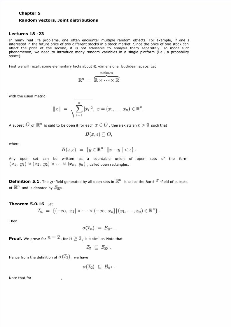
Chapter 5

Random vectors, Joint distributions

Lectures 18 -23

In many real life problems, one often encounter multiple random objects. For example, if one isnterested in the future price of two different stocks in a stock market. Since the price of one stock canaffect the price of the second, it is not advisable to analysis them separately. To model suchphenomenon, we need to introduce many random variables in a single platform (i.e., a probability

space).

First we will recall, some elementary facts about -dimensional Euclidean space. Let

with the usual metric

A subset of is said to be open if for each , there exists an such that

where

Any open set can be written as a countable union of open sets of the form

, called open rectangles.

Definition 5.1. The -field generated by all open sets in is called the Borel -field of subsets

of and is denoted by .

Theorem 5.0.16 Let

Then

Proof. We prove for , for , it is similar. Note that

Hence from the definition of , we have

Note that for ,



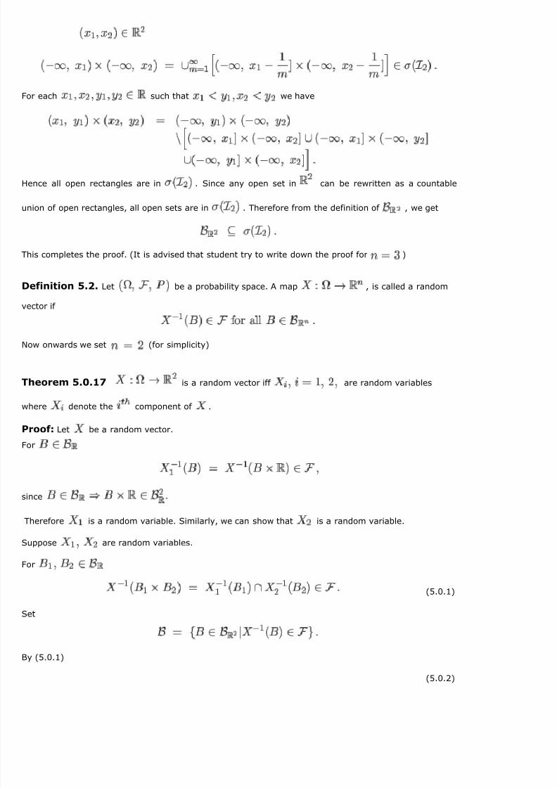
For each such that we have

Hence all open rectangles are in . Since any open set in can be rewritten as a countable

union of open rectangles, all open sets are in . Therefore from the definition of , we get

This completes the proof. (It is advised that student try to write down the proof for )

Definition 5.2. Let be a probability space. A map , is called a random

vector if

Now onwards we set (for simplicity)

Theorem 5.0.17 is a random vector iff are random variables

where denote the component of .

Proof: Let be a random vector.

For

since

Therefore is a random variable. Similarly, we can show that is a random variable.

Suppose are random variables.

For

(5.0.1)

Set

By (5.0.1)

(5.0.2)



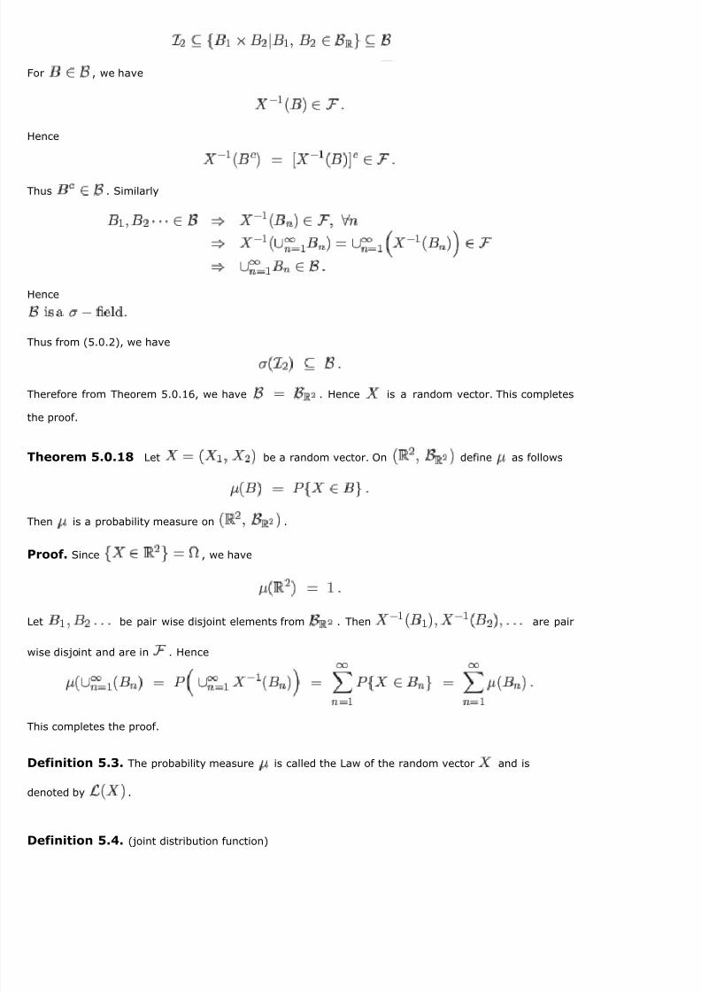
For , we have

Hence

Thus . Similarly

Hence

Thus from (5.0.2), we have

Therefore from Theorem 5.0.16, we have . Hence is a random vector. This completes

the proof.

Theorem 5.0.18 Let be a random vector. On define as follows

Then is a probability measure on .

Proof. Since , we have

Let be pair wise disjoint elements from . Then are pair

wise disjoint and are in . Hence

This completes the proof.

Definition 5.3. The probability measure is called the Law of the random vector and is

denoted by .

Definition 5.4. (joint distribution function)



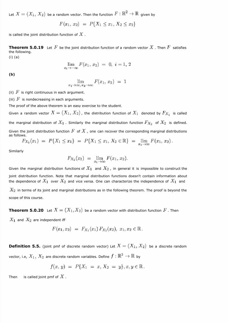
Let be a random vector. Then the function given by

s called the joint distribution function of .

Theorem 5.0.19 Let be the joint distribution function of a random vector . Then satisfies

the following.

(i) (a)

(b)

(ii) is right continuous in each argument.

(iii) is nondecreasing in each arguments.

The proof of the above theorem is an easy exercise to the student.

Given a random vector , the distribution function of denoted by is called

the marginal distribution of . Similarly the marginal distribution function of is defined.

Given the joint distribution function of , one can recover the corresponding marginal distributionsas follows.

Similarly

Given the marginal distribution functions of and , in general it is impossible to construct the

joint distribution function. Note that marginal distribution functions doesn't contain information about

the dependence of over and vice versa. One can characterize the independence of and

in terms of its joint and marginal distributions as in the following theorem. The proof is beyond the

scope of this course.

Theorem 5.0.20 Let be a random vector with distribution function . Then

and are independent iff

Definition 5.5. (joint pmf of discrete random vector) Let be a discrete random

vector, i.e, are discrete random variables. Define by

Then is called joint pmf of .



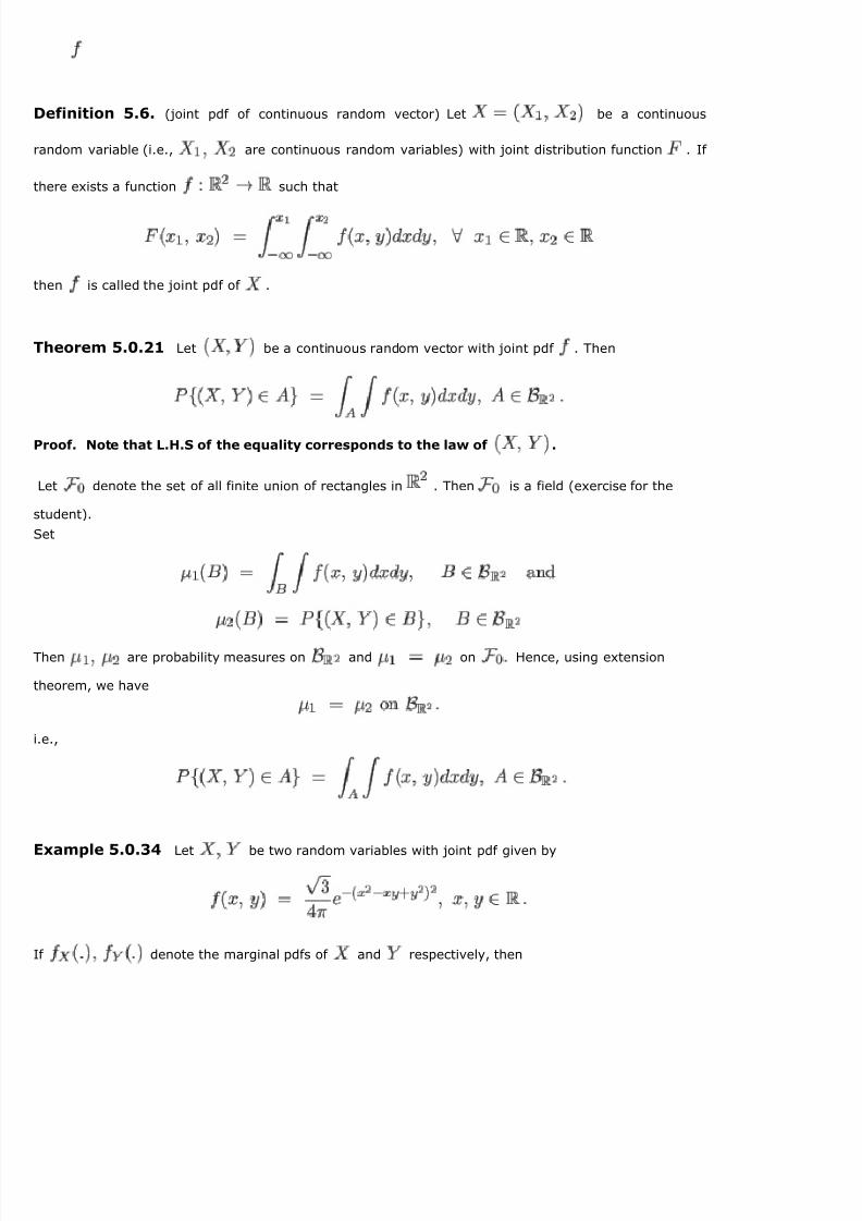
Definition 5.6. (joint pdf of continuous random vector) Let be a continuous

random variable (i.e., are continuous random variables) with joint distribution function . If

there exists a function such that

then is called the joint pdf of .

Theorem 5.0.21 Let be a continuous random vector with joint pdf . Then

Proof. Note that L.H.S of the equality corresponds to the law of .

Let denote the set of all finite union of rectangles in . Then is a field (exercise for the

student).

Set

Then are probability measures on and on Hence, using extension

theorem, we have

.e.,

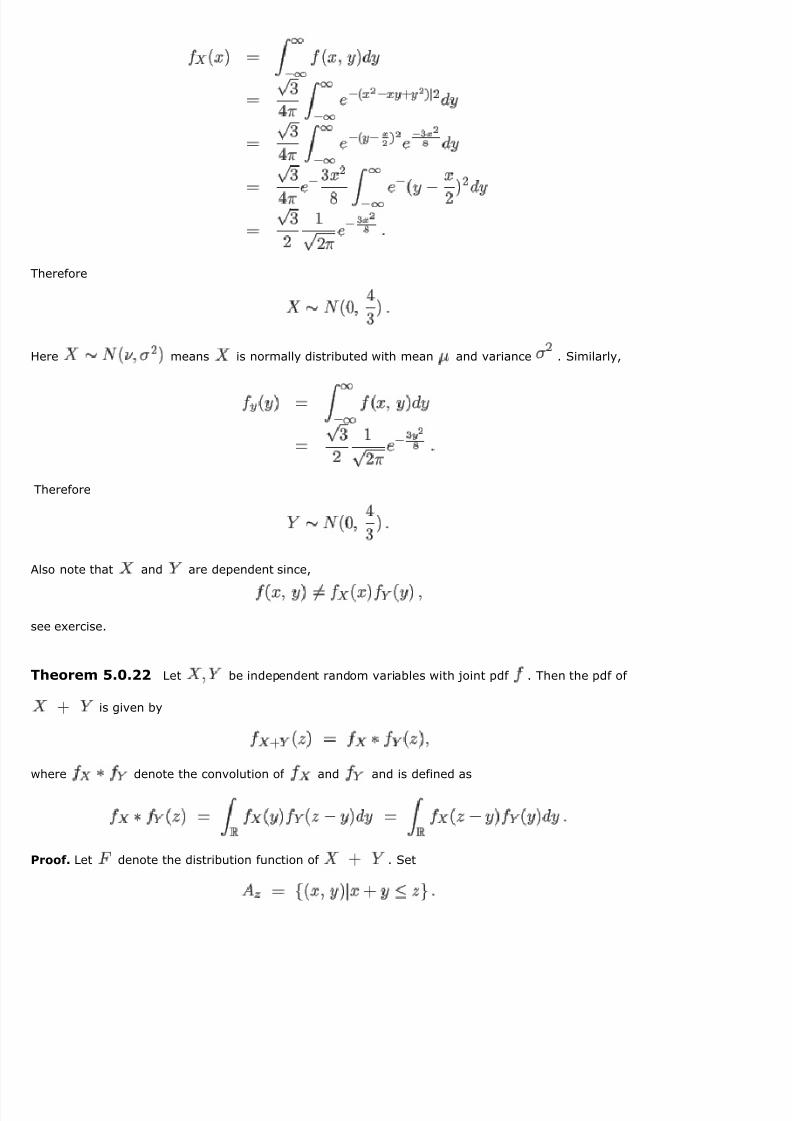
Example 5.0.34 Let be two random variables with joint pdf given by

If denote the marginal pdfs of and respectively, then



Therefore

Here means is normally distributed with mean and variance . Similarly,

Therefore

Also note that and are dependent since,

see exercise.

Theorem 5.0.22 Let be independent random variables with joint pdf . Then the pdf of

is given by

where denote the convolution of and and is defined as

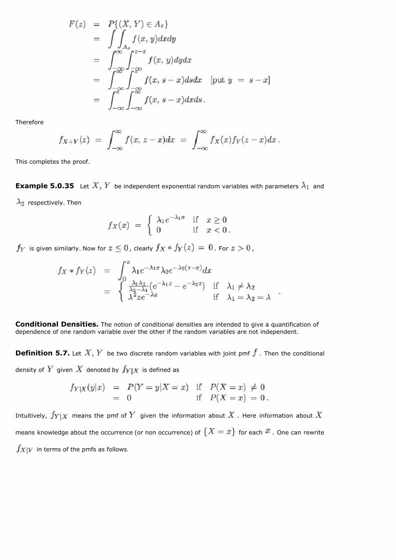
Proof. Let denote the distribution function of . Set



Therefore

This completes the proof.

Example 5.0.35 Let be independent exponential random variables with parameters and

respectively. Then

is given similarly. Now for , clearly . For ,

Conditional Densities. The notion of conditional densities are intended to give a quantification of

dependence of one random variable over the other if the random variables are not independent.

Definition 5.7. Let be two discrete random variables with joint pmf . Then the conditional

density of given denoted by is defined as

Intuitively, means the pmf of given the information about . Here information about

means knowledge about the occurrence (or non occurrence) of for each . One can rewrite

in terms of the pmfs as follows.



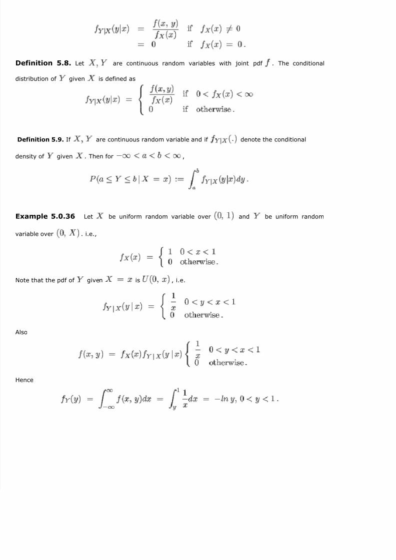
Definition 5.8. Let are continuous random variables with joint pdf . The conditional

distribution of given is defined as

Definition 5.9. If are continuous random variable and if denote the conditional

density of given . Then for ,

Example 5.0.36 Let be uniform random variable over and be uniform random

variable over . i.e.,

Note that the pdf of given is , i.e.

Also

Hence

Documents

Maths Probability Random vectors, Joint distributions lec5/8.pdf