Embed Size (px)
Citation preview

Mathematics of Seismic ImagingPart 1: Modeling and Inverse
Problems
William W. Symes
Rice University
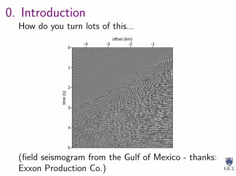
0. IntroductionHow do you turn lots of this...
0
1
2
3
4
5
time
(s)
-4 -3 -2 -1offset (km)
(field seismogram from the Gulf of Mexico - thanks:Exxon Production Co.)

0. Introductioninto this - an image of subsurface structure
0
500
1000
1500
2000
2500
Dep
th in
Met
ers
0 200 400 600 800 1000 1200 1400CDP
TRIP - K. Araya - 1995

0. Introductionresembling actual subsurface structure
WWS - 2013

0. Introduction
Also: what does imaging have to do with
inversion
= construction of a physical model that explainsdata
?
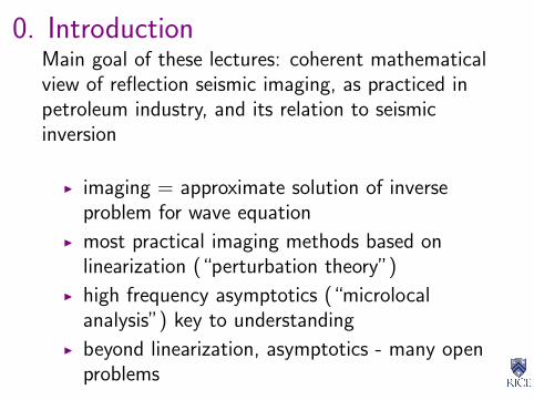
0. IntroductionMain goal of these lectures: coherent mathematicalview of reflection seismic imaging, as practiced inpetroleum industry, and its relation to seismicinversion
I imaging = approximate solution of inverseproblem for wave equation
I most practical imaging methods based onlinearization (“perturbation theory”)
I high frequency asymptotics (“microlocalanalysis”) key to understanding
I beyond linearization, asymptotics - many openproblems

0. Introduction
Lots of mathematics - much yet to becreated - with practical implications!

1. Modeling & Inverse Problems
1.1 Active Source Seismology
1.2 Wave Equations & Solutions
1.3 Inverse Problems

1. Modeling & Inverse Problems
1.1 Active Source Seismology
1.2 Wave Equations & Solutions
1.3 Inverse Problems

Reflection seismology
aka active source seismology, seismicsounding/profiling
uses seismic (elastic) waves to probe the Earth’ssedimentary crust
main exploration tool of oil & gas industry, alsoused in environmental and civil engineering (hazarddetection, bedrock profiling) and academicgeophysics (structure of crust and mantle)

Reflection seismology
highest resolution imaging technology for deepEarth exploration, in comparison with static(gravimetry, resistivity) or diffusive (passive, activesource EM) techniques - works because
waves transfer space-time resolved information fromone place to another with (relatively) little loss
wavelengths at easily accessible frequencies ∼ scaleof important structural features

Reflection seismology
Three components:
I energy/sound source - creates wave travelinginto subsurface
I receivers - record waves (echoes) reflected fromsubsurace
I recording and signal processing instrumentation

Reflection seismology
http://www.glossary.oilfield.slb.com/en/Terms/s/streamer.aspx, 12.07.2013

Reflection seismology
Marine reflection seismology:
I typical energy source: airgun array - releases(array of) supersonically expanding bubbles ofcompressed air, generates sound pulse in water
I typical receivers: hydrophones (waterproofmicrophones) in one or more 5-10 km flexiblestreamer(s) - wired together 500 - 30000groups (each group produces a single channel /time series)
I survey ships - lots of recording, processingcapacity

Reflection seismology
Survey consists of many experiments = shots =source positions xs
Simultaneous recording of reflections at manylocalized receivers, positions xr , time interval =0− O(10)s after initiation of source.
Data acquired on land and at sea (“marine”) - vastbulk (90%+) of data acquired each year is marine.

Reflection seismology
Marine seismic data parameters:
I time t - 0 ≤ t ≤ tmax, tmax = 5− 30s
I source location xs - 100 - 100000 distinctvalues
I receiver location xr
I typically the same range of offsets = xr − xs
for each shot - half offset h = xr−xs2 , h = |h|:
100 - 500000 values (typical: 5000) - few m to30 km (typical: 200 m - 8 km)
I data values: microphone output (volts), filteredversion of local pressure (force/area)

Reflection seismology
www.ogp.org.uk/pubs/448.pdf, 20.02.13

Reflection seismology
Acquisition “manifold”:
Idealized marine “streamer” geometry: xs and xr lieroughly on constant depth plane, source-receiverlines are parallel → 3 spatial degrees of freedom(eg. xs , h): codimension 1.
[Other geometries are interesting, eg. ocean bottomcables, but streamer surveys still prevalent.]

Reflection seismology
How much data? Contemporary surveys mayfeature
I Simultaneous recording by multiple streamers(up to 12!)
I Many (roughly) parallel ship tracks (“lines”)
I Recent development: Wide Angle TowedStreamer (WATS) survey - uses multiple surveyships for areal sampling of source and receiverpositions
I single line (“2D”) ∼ Gbytes; multiple lines(“3D”) ∼ Tbytes; WATS ∼ Pbytes

Reflection seismology
www.youtube.com/watch?v=vrOLWRVGosQ, 20.02.13

Distinguished data subsets
I traces = data for one source, one receiver:t 7→ d(xr , t; xs) - function of t, time series,single channel
I gathers or bins = subsets of traces, extractedfrom data after acquisition. Characterized bycommon value of an acquisition parameter

Distinguished data subsets
Examples:
I shot (or common source) gather: traces w/same shot location xs (previous expls)
I offset (or common offset) gather: traces w/same half offset h
I ...

Shot gather, Mississippi Canyon
0
1
2
3
4
5
time
(s)
-4 -3 -2 -1offset (km)
(thanks: Exxon)

Shot gather, Mississippi Canyon1.0
1.5
2.0
2.5
3.0
-2.5 -2.0 -1.5 -1.0 -0.5
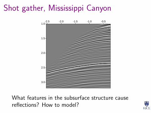
Lightly processed - bandpass filter 4-10-25-40 Hz,mute. Most striking visual characteristic: waves =coherent space-time structures (“reflections”)
Shot gather, Mississippi Canyon
1.0
1.5
2.0
2.5
3.0
-2.5 -2.0 -1.5 -1.0 -0.5
What features in the subsurface structure causereflections? How to model?

Well logs
1000 1200 1400 1600 1800 2000 2200 2400 2600 2800 3000500
1000
1500
2000
2500
3000
3500
4000
4500
depth (m)
Blocked logs from well in North Sea (thanks: MobilR & D). Solid: p-wave velocity (m/s), dashed:s-wave velocity (m/s), dash-dot: density (kg/m3).

Well logs
1000 1200 1400 1600 1800 2000 2200 2400 2600 2800 3000500
1000
1500
2000
2500
3000
3500
4000
4500
depth (m)
“Blocked” means “averaged” (over 30 m windows).Original sample rate of log tool < 1 m. Variance atall scales!

Well logs
0.5
1.0
1.5
2.0
2.5
Dep
th (k
m)
2 3 4 5Velocity (km/sec)
P-wave velocity log fromWest Texas
Thanks: Total E&P USA

Well logs
1000 1200 1400 1600 1800 2000 2200 2400 2600 2800 3000500
1000
1500
2000
2500
3000
3500
4000
4500
depth (m)
I Trends = slow increase in velocities, density -scale of km
I Reflectors = jumps in velocities, density -scale of m or 10s of m

1. Modeling & Inverse Problems
1.1 Active Source Seismology
1.2 Wave Equations & Solutions
1.3 Inverse Problems

The Modeling Task
A useful model of the reflection seismologyexperiment must
I predict wave motion
I produce reflections from reflectors
I accomodate significant variation of wavevelocity, material density,...

The Modeling Task
A really good model will also accomodate
I multiple wave modes, speeds
I material anisotropy
I attenuation, frequency dispersion of waves
I complex source, receiver characteristics

The Acoustic Model
Not really good, but good enough for this week andbasis of most contemporary seismicimaging/inversion
I ρ(x) = material density, κ(x) = bulk modulus
I p(x, t)= pressure, v(x, t) = particle velocity,
I f(x, t)= force density, g(x, t) = constitutivelaw defect (external energy source model)
The Acoustic Model
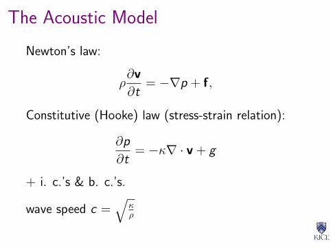
Newton’s law:
ρ∂v
∂t= −∇p + f,
Constitutive (Hooke) law (stress-strain relation):
∂p
∂t= −κ∇ · v + g
+ i. c.’s & b. c.’s.
wave speed c =√
κρ

The Acoustic Model
acoustic field potential u(x, t) =∫ t
−∞ ds p(x, s):
p =∂u
∂t, v =
1
ρ∇u
Equivalent form: second order wave equation forpotential
1
ρc2
∂2u
∂t2−∇· 1
ρ∇u =
g +
∫ t
−∞dt∇ ·
(f
ρ
)≡ f
ρ
plus initial, boundary conditions.

The Acoustic Model
Further idealizations:
I density ρ is constant,
I source force density is isotropic point radiatorwith known time dependence (“source pulse”w(t), typically of compact support)
f (x, t; xs) = w(t)δ(x− xs)
⇒ acoustic potential, pressure depends on sourcelocation xs also.

Homogeneous acousticsSuppose also that
I velocity c is constant
(“homogeneous” acoustic medium - samestress-strain relation everywhere)
Explicit causal ( = vanishing for t << 0) solutionfor 3D [Proof: exercise!]:
u(x, t) =w(t − r/c)
4πr, r = |x− xs |
Nomenclature: outgoing spherical wave

Homogeneous acoustics
Also explicit solution (up to quadrature) in 2D - abit more complicated (Poisson’s formula - exercise:find it! eg. in Courant and Hilbert)
Looks like expanding circular wavefront for typicalw(t)
[MOVIE 1]
Observe: no reflections!!!

Homogeneous acoustics
Upshot: if acoustic model is at all appropriate, mustuse non-constant c to explain observations.
Natural mathematical question: how nonconstantcan c be and still permit “reasonable” solutions ofwave equation?

Heterogeneous acoustics
Weak solution of Dirichlet problem in Ω ⊂ R3
(similar treatment for other b. c.’s):
u ∈ C 1([0,T ]; L2(Ω)) ∩ C 0([0,T ];H10 (Ω))
satisfying for any φ ∈ C∞0 ((0,T )× Ω),∫ T
0
∫Ω
dt dx
1
ρc2
∂u
∂t
∂φ
∂t− 1
ρ∇u · ∇φ +
1
ρf φ
= 0
Heterogeneous acoustics
Theorem (Lions, 1972) log ρ, log c ∈ L∞(Ω),f ∈ L2(Ω× R) ⇒ weak solutions of Dirichletproblem exist; initial data
u(·, 0) ∈ H10 (Ω),
∂u
∂t(·, 0) ∈ L2(Ω)
uniquely determine them.

Key Ideas in Proof
1. Conservation of energy: first assume that f ≡ 0,set
E [u](t) =1
2
∫Ω
(1
ρc2p(·, t)2 + ρ|v(·, t)|2
)= elastic strain energy (potential + kinetic)
=1
2
∫Ω
(1
ρc2
(∂u
∂t(·, t)
)2
+1
ρ|∇u(·, t)|2
)

Key Ideas in Proof
u smooth enough ⇒ integrations by parts &differentiations under integral sign make sense ⇒
dE [u]
dt= 0

Key Ideas in ProofGeneral case (f 6= 0): with help of Cauchy-Schwarz≤,
dE [u]
dt(t) ≤ const.
(E [u](t) +
∫ t
0
ds
∫Ω
dx f 2(x, s)
)whence for 0 ≤ t ≤ T ,
E [u](t) ≤ const.
(E [u](0) +
∫ t
0
ds
∫Ω
dx f 2(x, s)
)(Gronwall’s ≤)
const on RHS bounded by T ,‖ log ρ‖L∞(Ω), ‖ log c‖L∞(Ω)

Key Ideas in Proof
Poincare’s ≤ ⇒ “a priori estimate”∥∥∥∥∂u∂t (·, t)
∥∥∥∥L2(Ω)2
+ ‖u(·, t)‖2H1(Ω)
≤ const.
(∥∥∥∥∂u∂t (·, 0)
∥∥∥∥L2(Ω)2
+ ‖u(·, 0)‖2H1(Ω)
+
∫ t
−∞ds
∫Ω
dx f 2(x, s)
)

Key Ideas in Proof
Derivation presumed more smoothness than weaksolutions have, ex def. First serious result:
Weak solutions obey same a priori estimate
Proof via approximation argument.
Corollary: Weak solutions uniquely determined byt = 0 data

Key Ideas in Proof
2. Galerkin approximation: Pick increasing sequenceof subspaces
W 0 ⊂ W 1 ⊂ W 2 ⊂ ... ⊂ H10 (Ω)
so that∪∞n=0W
n dense in L2(Ω)
Typical example: piecewise linear Finite Elementsubspaces on sequence of meshes, each refinementof preceding.

Key Ideas in Proof
Galerkin principle: find un ∈ C 2([0,T ],W n) so thatfor any φn ∈ C 1([0,T ],W n),∫ T
0
∫Ω
dt dx
1
ρc2
∂un
∂t
∂φn
∂t− 1
ρ∇un · ∇φn +
1
ρf φn
= 0

Key Ideas in ProofIn terms of basis φnm : m = 0, ...,Nn of W n, write
un(t, x) =Nn∑m=0
Unm(t)φnm(x)
Then integration by parts in t ⇒ coefficient vectorUn(t) = (Un
0 (t), ...,UnNn)T satisfies ODE
Mnd2Un
dt2+ K nUn = F n
where
Mni ,j =
∫Ω
1
ρc2φni φ
nj , K
ni ,j =
∫Ω
1
ρ∇φni · ∇φnj
and sim for F n

Key Ideas in Proof
Assume temporarily thatf ∈ C 0([0,T ], L2(Ω)) ⊂ L2([0,T ]× Ω) - thenF n ∈ C 0([0,T ],W n), so...
basic theorem on ODEs ⇒ existence of Galerkinapproximation un.
Energy estimate for Galerkin approximation -
E [un](t) ≤ const.
(E [un](0) +
∫ t
0
‖f (·, t)‖2L2(Ω)
)constant independent of n.
Key Ideas in Proof
Alaoglu Thm ⇒ un weakly precompact inL2([0,T ],H1
0 (Ω)), ∂un/∂t weakly precompact inL2([0,T ], L2(Ω)), so can select weakly convergentsequence, limit u ∈ L2([0,T ],H1
0 (Ω)),∂u/∂t ∈ L2([0,T ], L2(Ω)).

Key Ideas in ProofFinal cleanup of Galerkin existence argument:
I u is weak solution (necessarily the weaksolution!)
I remove regularity assumption on f via densityof C 0([0,T ], L2(Ω)) in L2([0,T ]× Ω), energyestimate
More time regularity of f ⇒ more time regularity ofu. If you want more space regularity, thencoefficients must be more regular! (examples later)
See Stolk 2000 for details, Blazek et al. 2008 forsimilar results re symmetric hyperbolic systems

1. Modeling & Inverse Problems
1.1 Active Source Seismology
1.2 Wave Equations & Solutions
1.3 Inverse Problems

Reflection seismic inverse problem
Forward map F = time history of pressure foreach source location xs at receiver locations xr , asfunction of c
Reality: xs samples finitely many points near surfaceof Earth (z = 0), active receiver locations xr maydepend on source locations and are also discrete
but: sampling is reasonably fine (see plots!) so...
Idealization: (xs , xr) range over 4-diml closedsubmfd with boundary Σ, source and receiverdepths constant.

Reflection seismic inverse problem
(predicted seismic data), depends on velocity fieldc(x):
F [c] = p|Σ×[0,T ]
Inverse problem: given observed seismic datad ∈ L2(Σ× [0,T ]), find c so that
F [c] ' d
(NB: generalizations to elasticity etc., vectordata...)
Reflection seismic inverse problem
This inverse problem is
I large scale - Tbytes of data, Pflops to simulateforward map
I nonlinear
I yields to no known direct attack (no “solutionformula”)
I indirect approach: formulate as optimizationproblem (find “best fit” model)
Reflection seismic inverse problem
Optimization - typically least squares (Tarantola,Lailly,... 1980’s → present):
Given d , find c to minimize
‖F [c]− d‖2 [+regularization]
over suitable class of c
Contemporary alias: full waveform inversion(“FWI”)

Reflection seismic inverse problem
Changing attitudes to FWI:
I 2002: called “academic approach” byprominent exploration geophysicist
I 2013: every major oil and service company hassignificant R & D effort, some deployment
I SEG 2002: 2 technical sessions (out of > 50)inversion and other topics
I SEG 2012: 9 technical sessions on seismic FWI
I 3 major workshops in 2012-13

Reflection seismic inverse problem

Reflection seismic inverse problem
Size, cost ⇒ Newton relative ⇒ compute gradient(perhaps Hessian) - adjoint state method (Ch. 3)
⇒ linearization must make sense, i.e. F must bedifferentiable in some sense