Embed Size (px)
Citation preview
Mathematics of Machine LearningMathematics of Machine Learning
Optimization strategies for supervised learningOptimization strategies for supervised learning
OverviewOverview
From learning to OptimizationIntroduction to OptimizationCurrent trends
Supervised learningSupervised learning
Given �nd a function such that
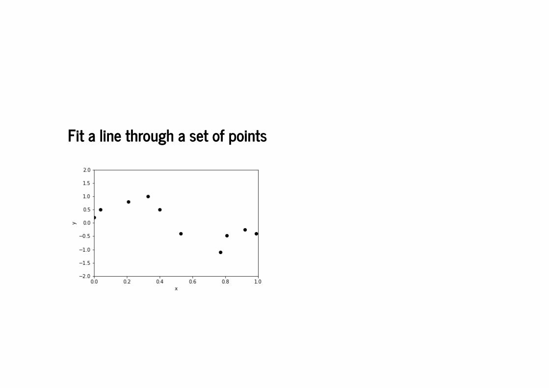
Fit a line through a set of pointsFit a line through a set of points
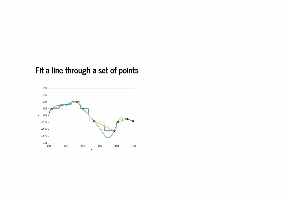
Fit a line through a set of pointsFit a line through a set of points
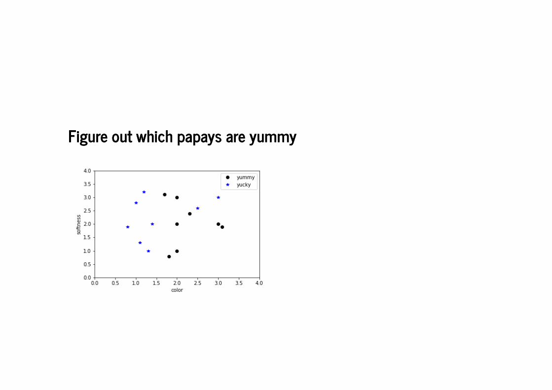
Figure out which papays are yummyFigure out which papays are yummy
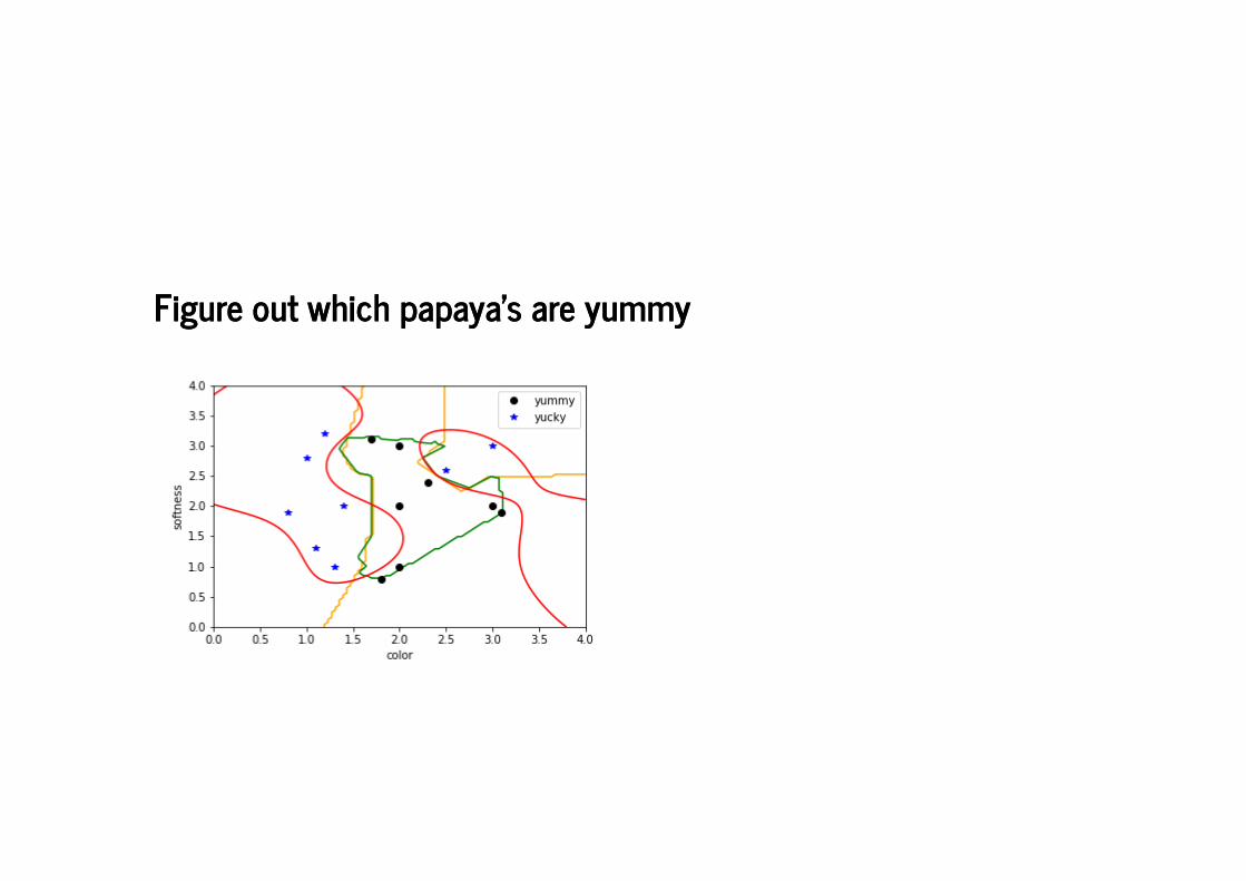
Figure out which papaya's are yummyFigure out which papaya's are yummy
The supervised learning zooThe supervised learning zoo
RegressionNeural networksSupport Vector Machines....
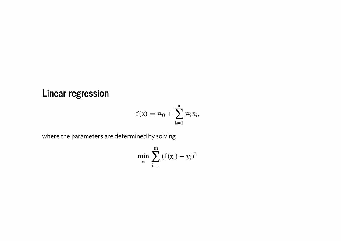
Linear regressionLinear regression
where the parameters are determined by solving
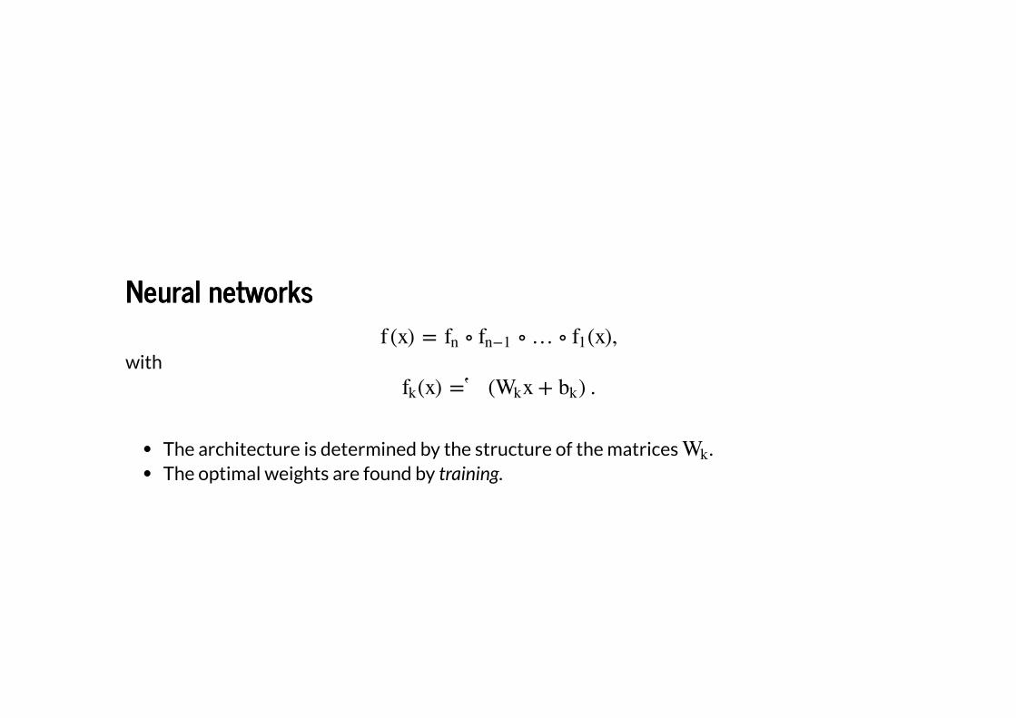
Neural networksNeural networks
with
The architecture is determined by the structure of the matrices .The optimal weights are found by training.
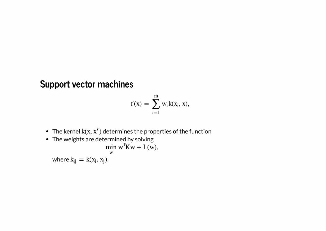
Support vector machinesSupport vector machines
The kernel determines the properties of the functionThe weights are determined by solving
where .
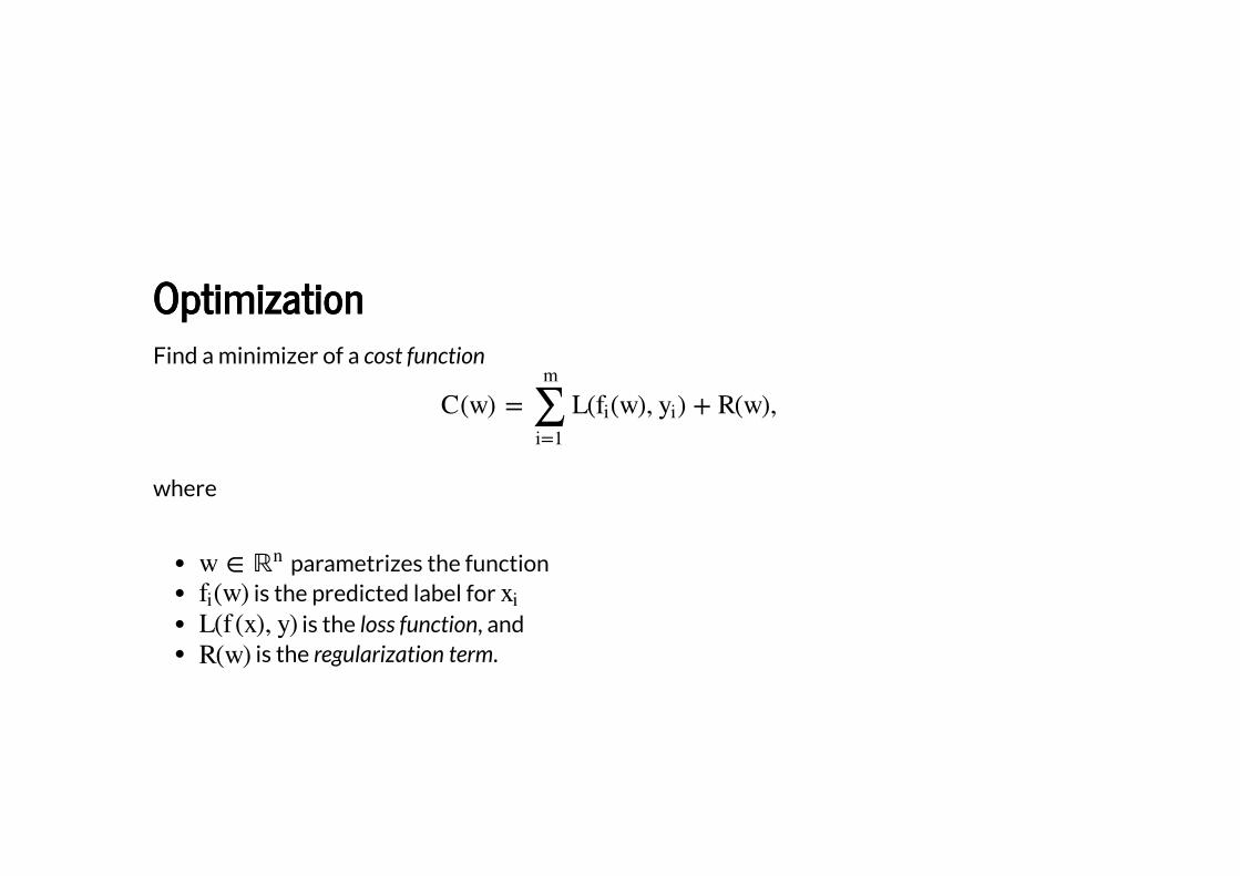
OptimizationOptimization
Find a minimizer of a cost function
where
parametrizes the function is the predicted label for
is the loss function, and is the regularization term.
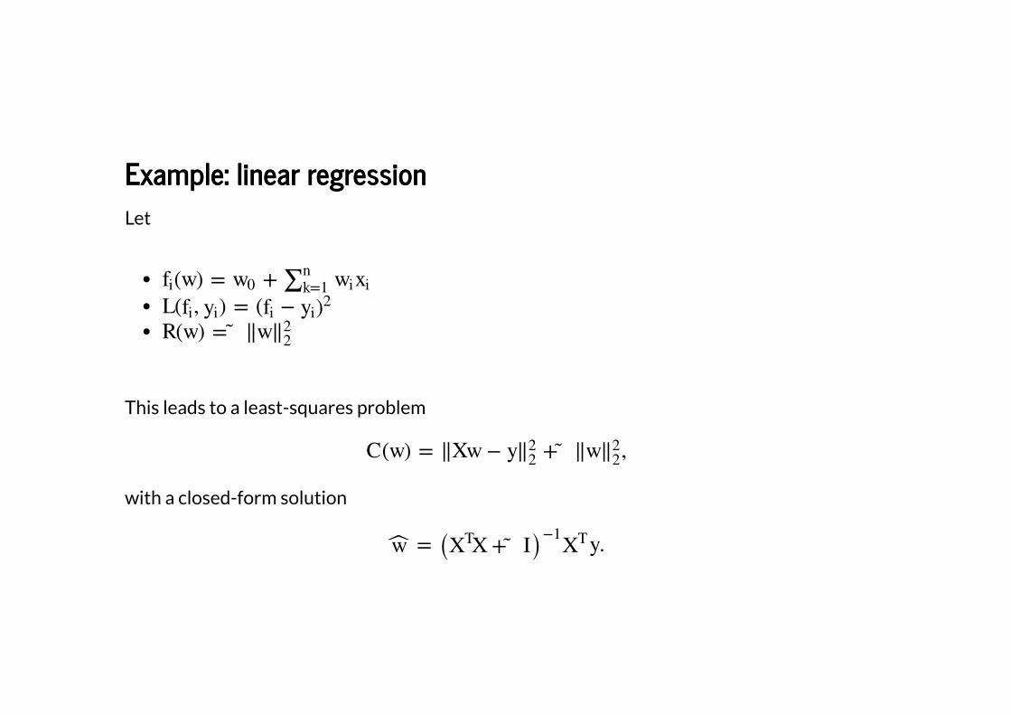
Example: linear regressionExample: linear regression
Let
This leads to a least-squares problem
with a closed-form solution
OptimizationOptimization
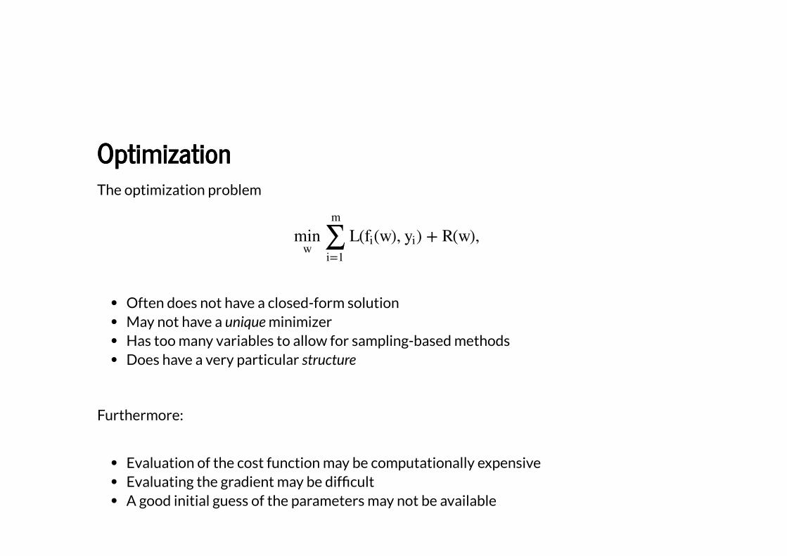
The optimization problem
Often does not have a closed-form solutionMay not have a unique minimizerHas too many variables to allow for sampling-based methodsDoes have a very particular structure
Furthermore:
Evaluation of the cost function may be computationally expensiveEvaluating the gradient may be dif�cultA good initial guess of the parameters may not be available
OptimizationOptimization
Structure of the cost functionOptimality conditionsBasic iterative algorithms
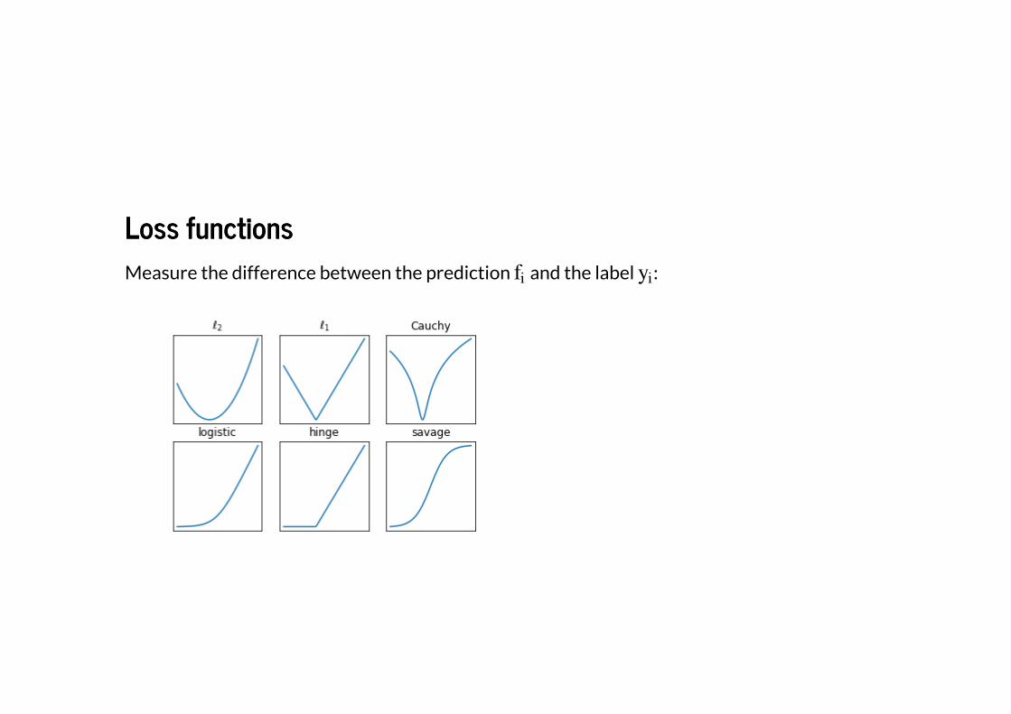
Loss functionsLoss functions
Measure the difference between the prediction and the label :
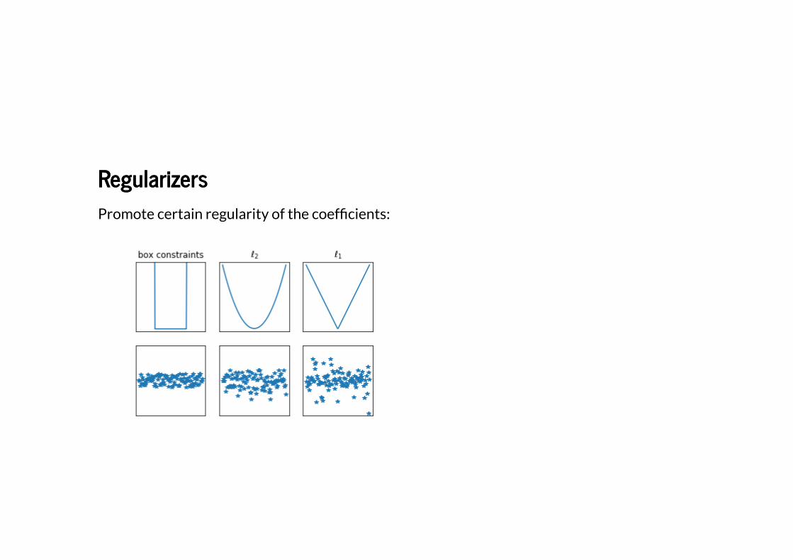
RegularizersRegularizers
Promote certain regularity of the coef�cients:
De�ning propertiesDe�ning properties
Three properties come up frequently in optimization:
ContinuityConvexitySmoothness
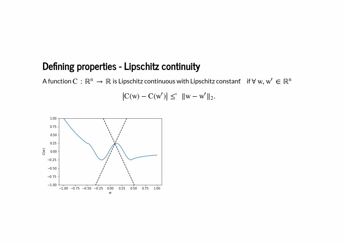
De�ning properties - Lipschitz continuityDe�ning properties - Lipschitz continuity
A function is Lipschitz continuous with Lipschitz constant if
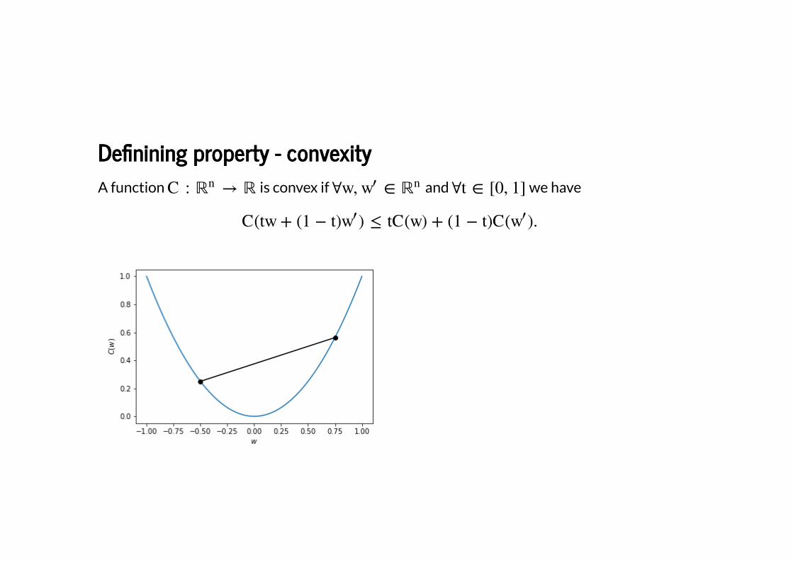
De�nining property - convexityDe�nining property - convexity
A function is convex if and we have
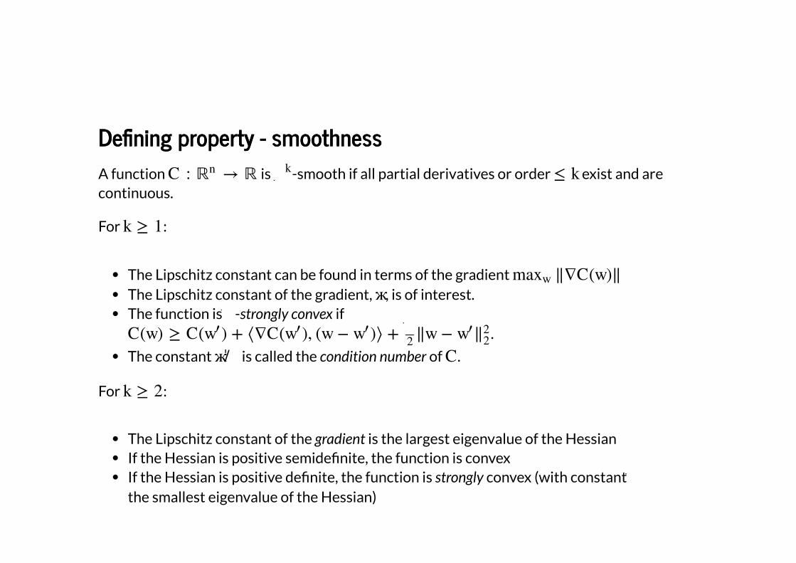
De�ning property - smoothnessDe�ning property - smoothness
A function is -smooth if all partial derivatives or order exist and arecontinuous.
For :
The Lipschitz constant can be found in terms of the gradient The Lipschitz constant of the gradient, , is of interest.The function is -strongly convex if
.
The constant is called the condition number of .
For :
The Lipschitz constant of the gradient is the largest eigenvalue of the HessianIf the Hessian is positive semide�nite, the function is convexIf the Hessian is positive de�nite, the function is strongly convex (with constant the smallest eigenvalue of the Hessian)
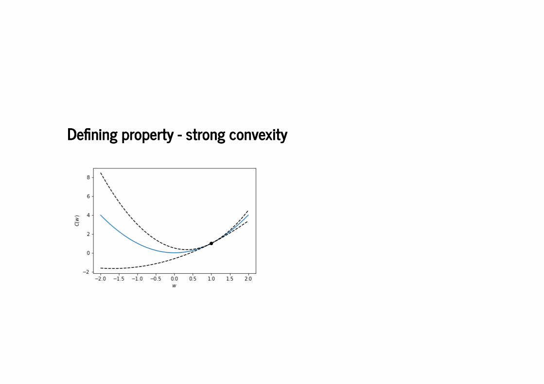
De�ning property - strong convexityDe�ning property - strong convexity
De�ning propertiesDe�ning properties
Note:
It is often not possible to �nd the (global) bounds a-prioriThe objective may not be globally convex/strongly convex, but is usefull to think ofthese as local properties that hold close to a minimizer
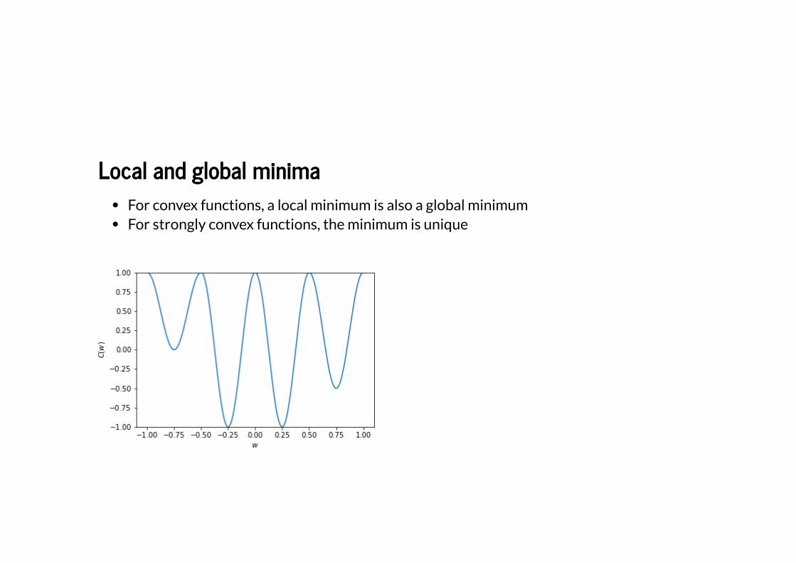
Local and global minimaLocal and global minima
For convex functions, a local minimum is also a global minimumFor strongly convex functions, the minimum is unique
Optimality conditions (for local minima)Optimality conditions (for local minima)
Smooth function:
Gradient is zero, Hessian is positive (semi-)de�nite
Convex function:
Subgradient contains zero
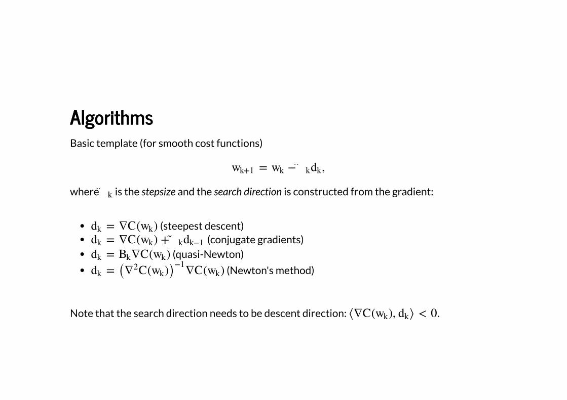
AlgorithmsAlgorithms
Basic template (for smooth cost functions)
where is the stepsize and the search direction is constructed from the gradient:
(steepest descent) (conjugate gradients)
(quasi-Newton)
(Newton's method)
Note that the search direction needs to be descent direction: .
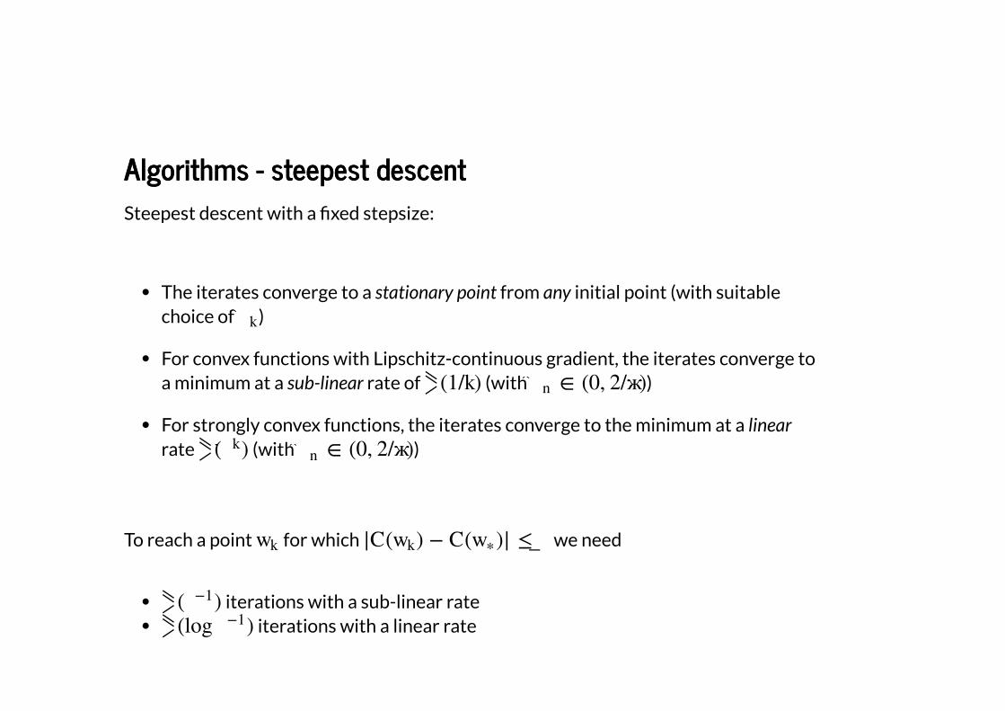
Algorithms - steepest descentAlgorithms - steepest descent
Steepest descent with a �xed stepsize:
The iterates converge to a stationary point from any initial point (with suitablechoice of )
For convex functions with Lipschitz-continuous gradient, the iterates converge toa minimum at a sub-linear rate of (with )
For strongly convex functions, the iterates converge to the minimum at a linearrate (with )
To reach a point for which we need
iterations with a sub-linear rate iterations with a linear rate
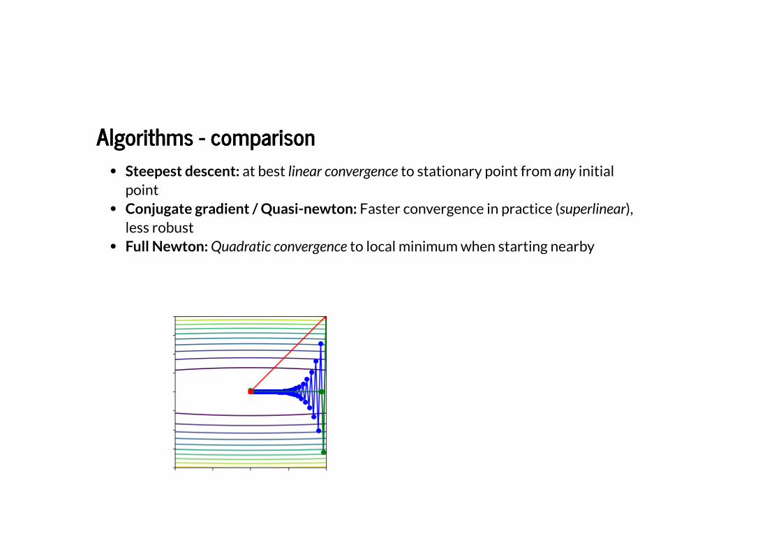
Algorithms - comparisonAlgorithms - comparison
Steepest descent: at best linear convergence to stationary point from any initialpointConjugate gradient / Quasi-newton: Faster convergence in practice (superlinear),less robustFull Newton: Quadratic convergence to local minimum when starting nearby
Algorithms - comparisonAlgorithms - comparison
In practice we need to trade-off convergence rates, robustness and computational cost:
Steepest descent has cheap iterationsQuasi-Newton typically requires some storage to build up curvature informationFull Newton requires the solution of a large system of linear equations at eachiteration
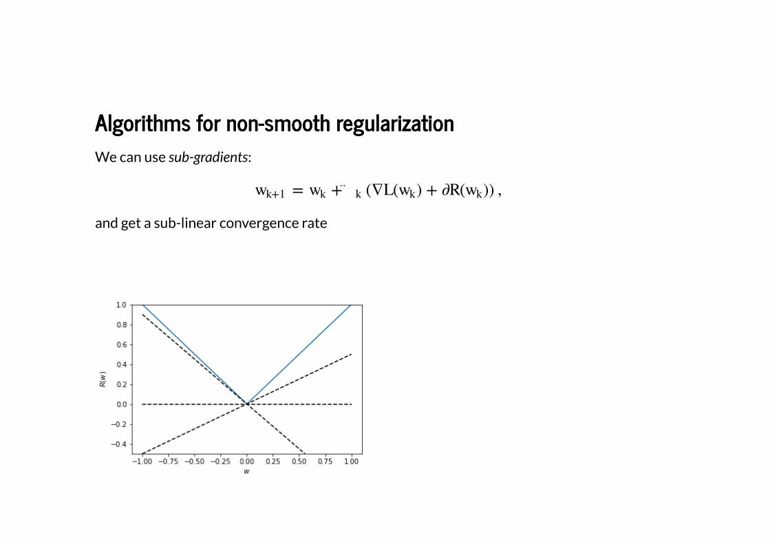
Algorithms for non-smooth regularizationAlgorithms for non-smooth regularization
We can use sub-gradients:
and get a sub-linear convergence rate
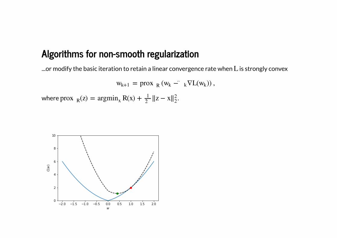
Algorithms for non-smooth regularizationAlgorithms for non-smooth regularization
...or modify the basic iteration to retain a linear convergence rate when is strongly convex
where .
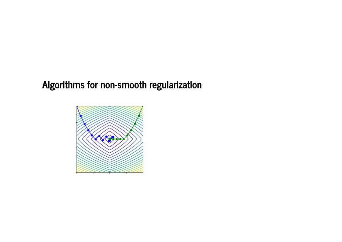
Algorithms for non-smooth regularizationAlgorithms for non-smooth regularization
Algorithms for non-smooth regularizationAlgorithms for non-smooth regularization
Note that when is the indicator of a convex set, the proximal operator projects onto theconvex set.
Box-constraints : 2-norm ball : 1-norm ball :
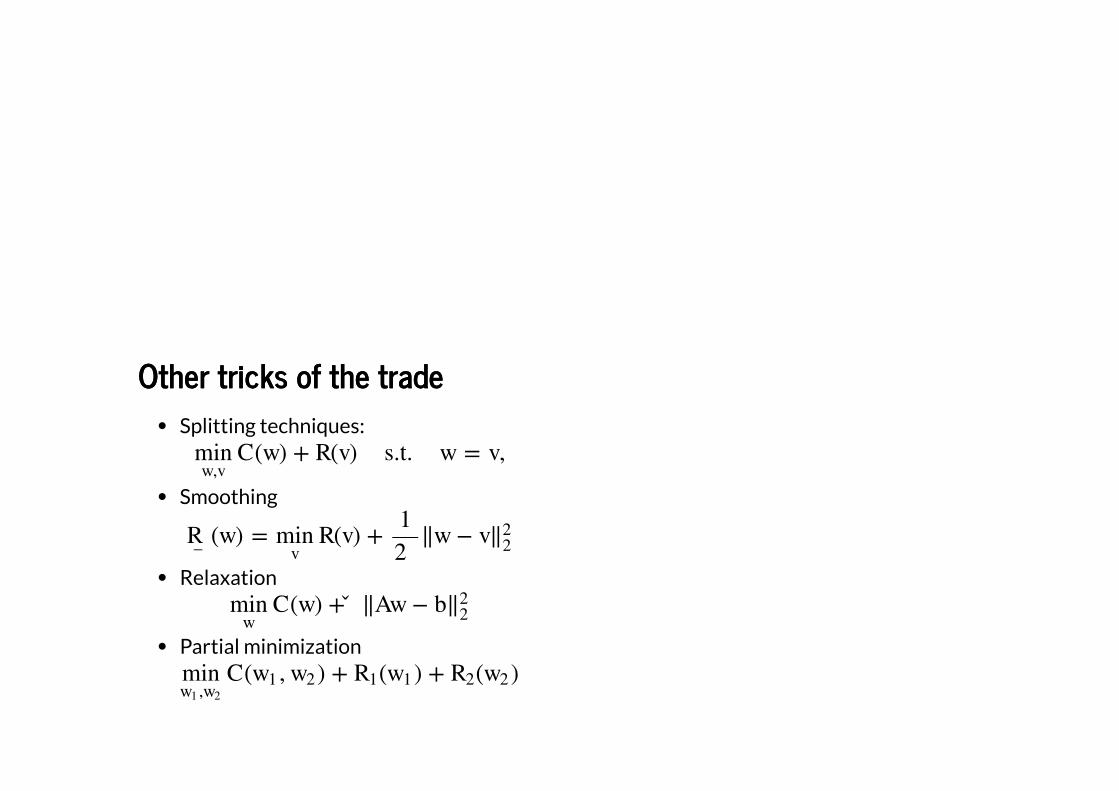
Other tricks of the tradeOther tricks of the trade
Splitting techniques:
Smoothing
Relaxation
Partial minimization
Some practical issuesSome practical issues
Bias-variance trade-offVanishing/exploding gradient in RNN's
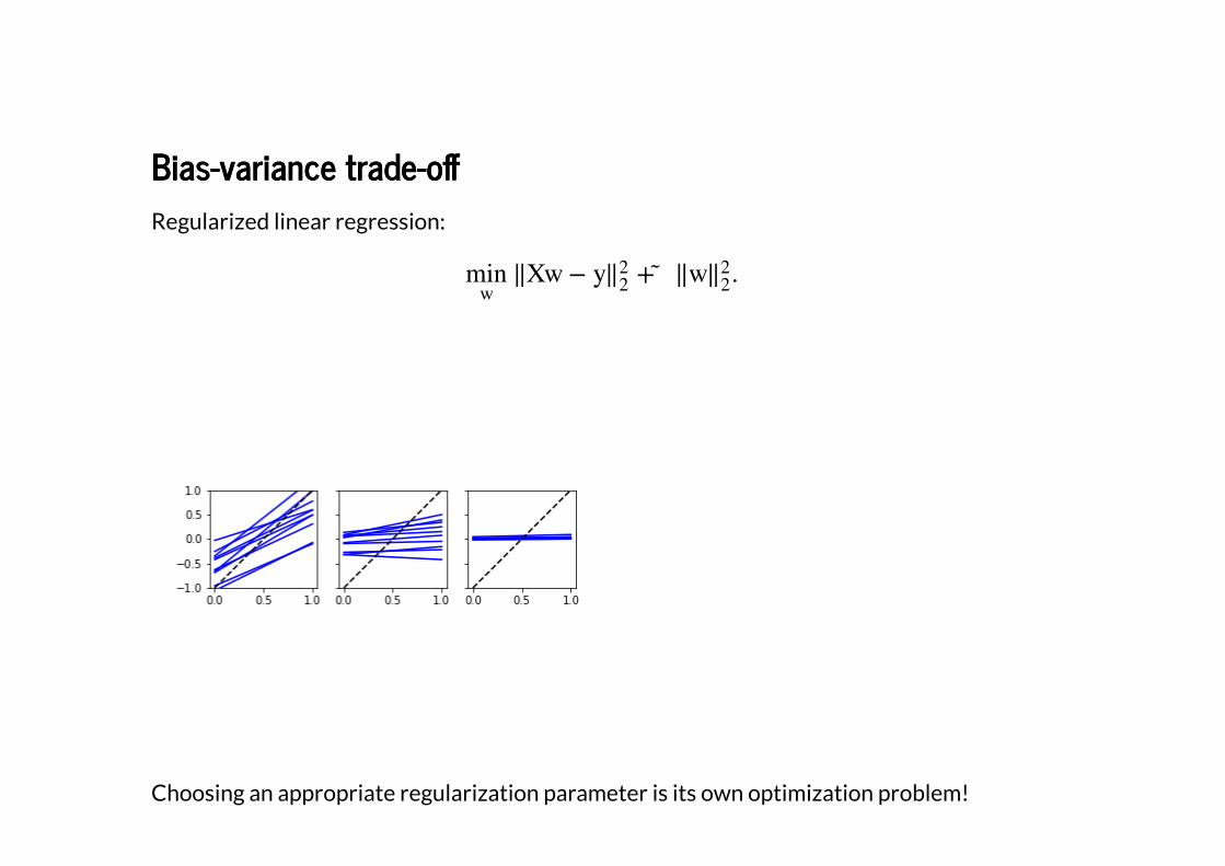
Bias-variance trade-o�Bias-variance trade-o�
Regularized linear regression:
Choosing an appropriate regularization parameter is its own optimization problem!
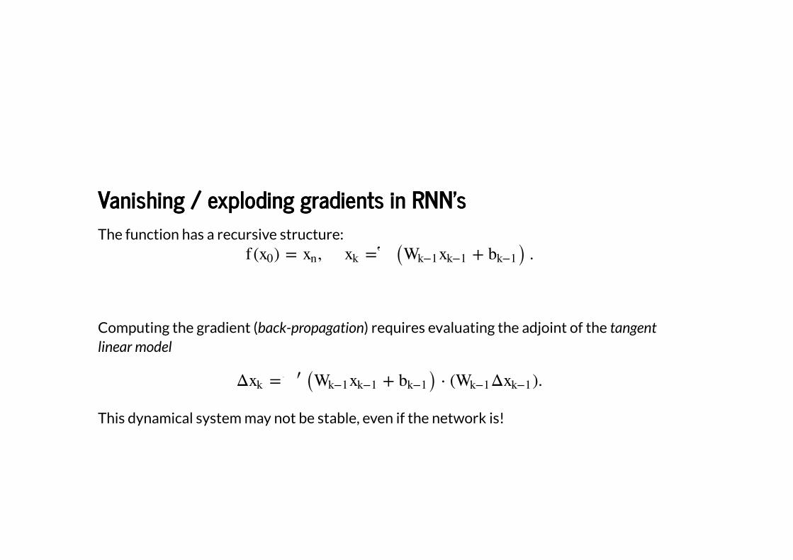
Vanishing / exploding gradients in RNN'sVanishing / exploding gradients in RNN's
The function has a recursive structure:
Computing the gradient (back-propagation) requires evaluating the adjoint of the tangentlinear model
This dynamical system may not be stable, even if the network is!
Some current trendsSome current trends
Stochastic optimization and accelerationVisualization/insight
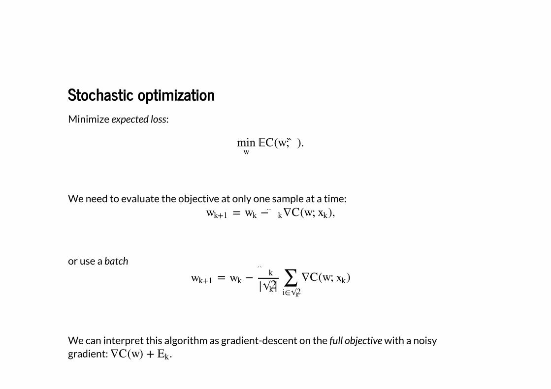
Stochastic optimizationStochastic optimization
Minimize expected loss:
We need to evaluate the objective at only one sample at a time:
or use a batch
We can interpret this algorithm as gradient-descent on the full objective with a noisygradient: .
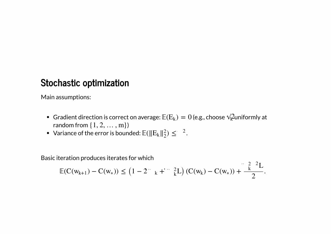
Stochastic optimizationStochastic optimization
Main assumptions:
Gradient direction is correct on average: (e.g., choose uniformly atrandom from )Variance of the error is bounded: .
Basic iteration produces iterates for which
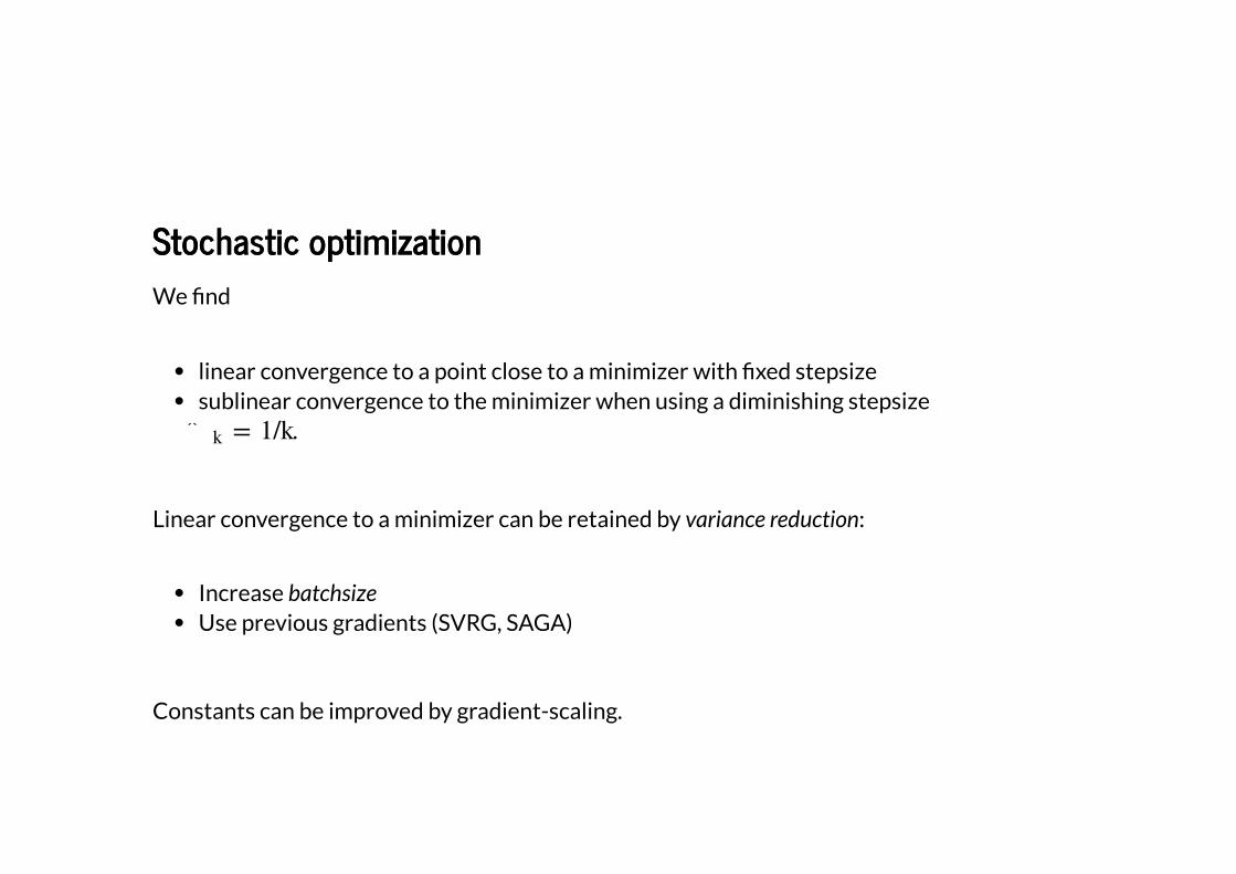
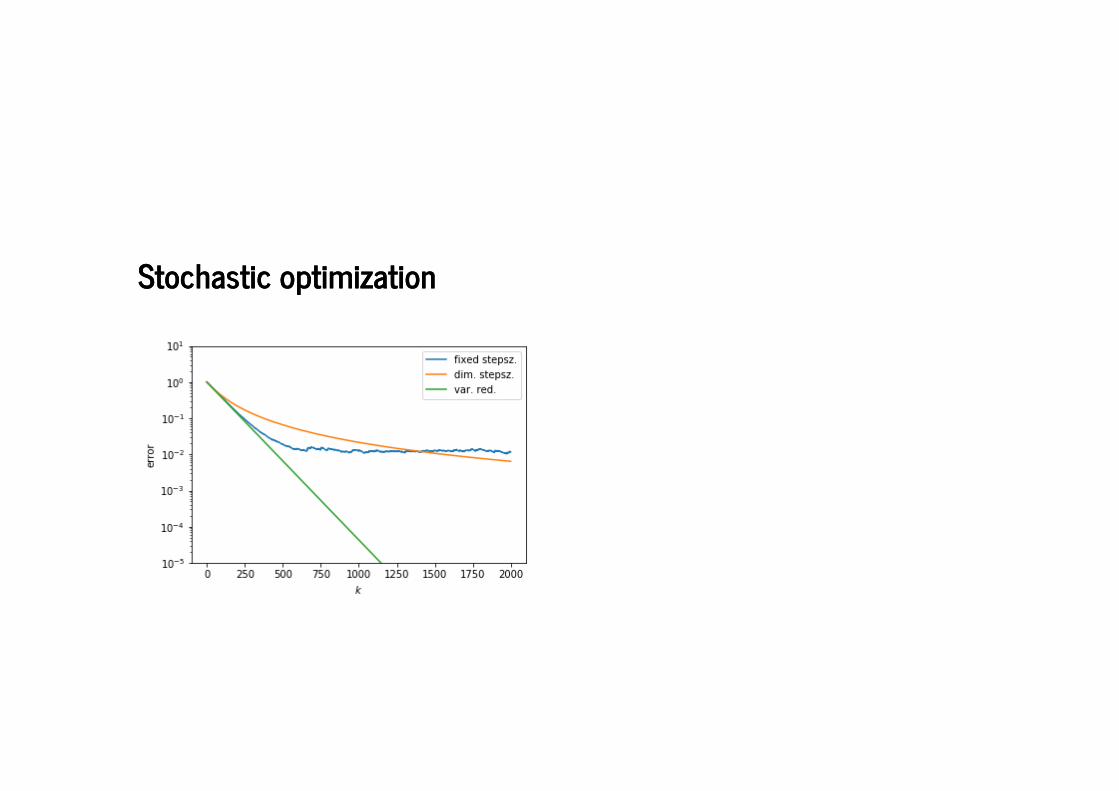
Stochastic optimizationStochastic optimization
We �nd
linear convergence to a point close to a minimizer with �xed stepsizesublinear convergence to the minimizer when using a diminishing stepsize
.
Linear convergence to a minimizer can be retained by variance reduction:
Increase batchsizeUse previous gradients (SVRG, SAGA)
Constants can be improved by gradient-scaling.
Stochastic optimizationStochastic optimization
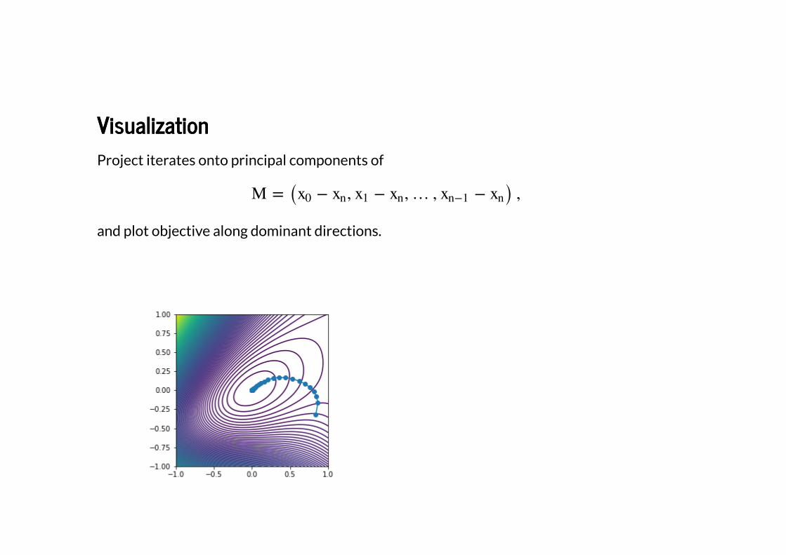
VisualizationVisualization
Project iterates onto principal components of
and plot objective along dominant directions.
SummarySummary
Supervised learning leads to interesting and structured optimization problemsMany specialized algorithms are available to take advantage of this structureStochastic methods can be usefully analyzed as gradient-descent-with-errors
Further readingFurther reading
Extensive overview of optimization methods (http://ruder.io/optimizing-gradient-descenAnother extensive overview(https://www.researchgate.net/pro�le/Frank_E_Curtis/publication/303992986_OptimizScale_Machine_Learning/links/5866da5908aebf17d39aeba7/Optimization-Methods-foLearning.pdf)The effect of regularization in classi�cation (https://thomas-tanay.github.io/post--L2-regWell-posed network architectures (https://arxiv.org/pdf/1705.03341.pdf)Visualizing the loss (https://arxiv.org/pdf/1712.09913.pdf)Partial minimization (https://arxiv.org/abs/1601.05011)