Embed Size (px)
Citation preview
Mathematical problems of General Relativity
Juan A. Valiente Kroon
School of Mathematical SciencesQueen Mary, University of London
LTCC Course LMS
Juan A. Valiente Kroon (QMUL) Mathematical GR 1 / 57
Outline of the course
Outline
1 Outline of the course
2 A review of Differential GeometryBasic notionsManifolds with metric
3 A brief survey of General RelativityBasic notionsExact solutions
4 The Einstein equation as a wave equationThe scalar wave equationThe Maxwell equations as wave equationsThe Einstein equations in wave coordinates
Juan A. Valiente Kroon (QMUL) Mathematical GR 2 / 57
Outline of the course
Objectives and content
Objectives:
Provide a discussion of General Relativity as an initial value problem.
Provide an introduction to applied methods of Differential Geometry andpartial differential equations.
Give an overview of main ideas and methods of mathematical GeneralRelativity;
Topics to be covered
1 A review of Differential Geometry
2 A survey of General Relativity
3 The Einstein equation as a wave equation
4 The 3 + 1 decomposition of General Relativity
5 The constraint equations of General Relativity
6 The ADM evolution equations
7 Time independent solutions
8 Energy and momentum in General Relativity (if time permits)Juan A. Valiente Kroon (QMUL) Mathematical GR 3 / 57
Outline of the course
Resources and further material
Notes:
Available at: www.maths.qmul.ac.uk/∼jav/LTCC
These include notes of the lectures, slides and an extended overview ofDifferential Geometry —all comments abut these welcome!
Problems:
4 problem sheets will be provided.
Mainly to elaborate one calculations briefly discussed in the lectures.
Assessment
The course contains a light assessment consisting of a problem sheet to take homeand to be handed back two weeks after.
Juan A. Valiente Kroon (QMUL) Mathematical GR 4 / 57

Outline of the course
About me
About me:
(Bsc Physics/Maths)
(PhD in General Relativity)
(1st postdoc)(2nd postdoc)
(Reader)(Advanced Research Fellow)
Thursday, 14 February 2013Juan A. Valiente Kroon (QMUL) Mathematical GR 5 / 57
A review of Differential Geometry
Outline
1 Outline of the course
2 A review of Differential GeometryBasic notionsManifolds with metric
3 A brief survey of General RelativityBasic notionsExact solutions
4 The Einstein equation as a wave equationThe scalar wave equationThe Maxwell equations as wave equationsThe Einstein equations in wave coordinates
Juan A. Valiente Kroon (QMUL) Mathematical GR 6 / 57
A review of Differential Geometry Basic notions
Outline
1 Outline of the course
2 A review of Differential GeometryBasic notionsManifolds with metric
3 A brief survey of General RelativityBasic notionsExact solutions
4 The Einstein equation as a wave equationThe scalar wave equationThe Maxwell equations as wave equationsThe Einstein equations in wave coordinates
Juan A. Valiente Kroon (QMUL) Mathematical GR 7 / 57
A review of Differential Geometry Basic notions
Manifolds (I)
Definition:
The basic concept in Differential Geometry is that of a differentiablemanifold (or manifold for short).
A manifold M is essentially a (topological) space that can be covered by acollection of charts (U , φ) where U ⊂M is an open subset and φ : U → Rnfor some n is a smooth injective (one-to-one) mapping.
The notion of a manifold requires certain compatibility between overlappingcharts.
In what follows, for simplicity and unless otherwise stated, it is assumed thatall structures are smooth.
Attention will be restricted to manifolds of dimensions 4 and 3.
Juan A. Valiente Kroon (QMUL) Mathematical GR 8 / 57
A review of Differential Geometry Basic notions
Manifolds (II)
Local coordinates:
Given p ∈ U one writesφ(p) = (x1, . . . , xn).
The (xµ) = (x1, . . . , xn) are called the local coordinates on U .
Orientability:
A manifold M is said to be orientable if the Jacobian of the transformationbetween overlapping charts is positive.
Scalar fields over a manifold:
A scalar field over M is a smooth function f :M→ R. The set of scalar fieldsover M will be denoted by X(M).
Juan A. Valiente Kroon (QMUL) Mathematical GR 9 / 57
A review of Differential Geometry Basic notions
Curves on manifold
Definition:
A curve is a smooth map γ : I →M with I ⊂ R.
In terms of coordinates (xµ) defined over a chart of M one writes the curveas
xµ(λ) = (x1(λ), . . . , xn(λ)),
where λ ∈ I is the parameter of the curve.
Juan A. Valiente Kroon (QMUL) Mathematical GR 10 / 57
A review of Differential Geometry Basic notions
Vectors on a manifold (I)
Tangent vector:
The concept of tangent vector formalises the physical notion of velocity.
In local coordinates, the tangent vector to the curve xµ(λ) is given by
vµ =dxµ
dλ.
In modern Differential Geometry one identifies vectors with homogeneousfirst order differential operators acting on scalar fields over M.
This approach allow to encode in a simple manner the classicaltransformation properties of vectors between charts.
Following this perspective, in local coordinates a vector field will be written as
vµ∂µ.
Juan A. Valiente Kroon (QMUL) Mathematical GR 11 / 57
A review of Differential Geometry Basic notions
Vectors on a manifold (II)
Abstract index notation:
In what follows we will mostly make use of the abstract index notation todenote vectors and tensors.
A generic vector will in this formalism denoted as va.
The role of the superindex in this notation is to indicate the character of theobject in question.
For the components in some coordinate system (xµ) write vµ.
Tangent space and tangent bundle:
The set of vectors at a point p of M is the tangent space at p, TpM.
A (smooth) prescription of a vector at every point of M is called a vectorfield.
The collection of all tangent spaces onM is called the tangent bundle TM.
Juan A. Valiente Kroon (QMUL) Mathematical GR 12 / 57
A review of Differential Geometry Basic notions
Covectors
Definition:
A covector (or 1-form) is real valued function of a vector.
In abstract index notation denoted by ωa.
The action of ωa on va will be denoted by ωava ∈ X(M).
Cotangent space
The set of covectors at a point p ∈M is the cotangent space T ∗pM.
The set of all cotangent spaces on M is the cotangent bundle T ∗M.
Juan A. Valiente Kroon (QMUL) Mathematical GR 13 / 57
A review of Differential Geometry Basic notions
Higher rank tensors
Definition:
Higher rank objects (tensors) can be constructed by analogy.
A tensor of type (m,n) is a real-valued functions of m covectors and nvectors that are linear in all their arguments.
For example, the tensor T abc is of type (2, 1).
Traditionally, superindices in a tensor are called contravariant whilesubindices ones are called covariant.
Symmetric and antisymmetric tensors:
A tensor is symmetric if it remains unchanged under the interchange of twoof its arguments Tab = Tba.
A tensor is antisymmetric if it changes sign with an interchange of a pair ofarguments as in Sabc = −Sacb.The symmetric and antisymmetric parts of a tensor can be constructed byadding together all possible permutations with the appropriate signs. Forexample
T(ab) = 12 (Tab + Tba), T[ab] = 1
2 (Tab − Tba).Juan A. Valiente Kroon (QMUL) Mathematical GR 14 / 57
A review of Differential Geometry Manifolds with metric
Outline
1 Outline of the course
2 A review of Differential GeometryBasic notionsManifolds with metric
3 A brief survey of General RelativityBasic notionsExact solutions
4 The Einstein equation as a wave equationThe scalar wave equationThe Maxwell equations as wave equationsThe Einstein equations in wave coordinates
Juan A. Valiente Kroon (QMUL) Mathematical GR 15 / 57
A review of Differential Geometry Manifolds with metric
Metric tensors (I)
Definition:
A metric on M is a non-degenerate symmetric (0, 2) tensor field gab.
Non-degenerate: if gabuavb = 0 for all ua if and only if va = 0.
The metric encodes the geometric notions of orthogonality and norm of avector.
The norm of a vector is given by |v|2 = gabvavb
If gabvaua = 0, then va and ua are said to be orthogonal.
Riemannian and Lorentzian metrics
In terms of a coordinate system (xµ) the components of gab, gµν , are a n× nmatrix. Because of symmetry, this matrix has n real eigenvalues.
The signature of gab is the difference between the number of positive andnegative eigenvalues.
If the signature is ±n then one has a Riemannian metric.
If the signature is ±(n− 2) then the metric is said to be Lorentzian.
Juan A. Valiente Kroon (QMUL) Mathematical GR 16 / 57
A review of Differential Geometry Manifolds with metric
Metric tensors (II)
Index gymnastics:
A metric gab can be used to define a one-to-one correspondence betweenvectors and covectors.
In local coordinates denote by gµν the inverse of gµν . This defines a (2, 0)tensor which we denote by gab.
By construction gabgbc = δa
c where δac is the Kroneker delta.
Given a vector va one defines va ≡ gabva.
Similarly, given a covector ωa one can define ωa ≡ gabωb.
Juan A. Valiente Kroon (QMUL) Mathematical GR 17 / 57
A review of Differential Geometry Manifolds with metric
Remarks for Lorentzian metrics
Classifying vectors according to their causal nature:
In these lectures all Lorentzian metrics will be defined on a 4-dimensionalmanifold and will be assumed to have signature 2 —that is, one has onenegative eigenvalue and 3 positive ones.
A Lorentzian metric can be used to classify vectors according to the sign oftheir norm.
va is said to be timelike if gabvavb < 0;
va is said to be null if gabvavb = 0;
va is said to be spacelike if gabvavb > 0.
Juan A. Valiente Kroon (QMUL) Mathematical GR 18 / 57
A review of Differential Geometry Manifolds with metric
The Levi-Civita connection (I)
Covariant derivatives
A covariant derivative is a notion of derivative with tensorial properties.
A metric gab allows to define a covariant derivative ∇a over M —theso-called Levi-Civita connection.
The covariant derivative of a vector va is denoted by ∇avb. For a covectorωb one writes ∇aωb.
The Christoffel symbols
Explicit formulae in terms of local coordinates involve the so-calledChristoffel symbols
Γµνλ = 12gµρ(∂νgρλ + ∂λgνρ − ∂ρgνλ).
Notice that Γµνλ = Γµλν .
The Christoffel symbols do not define a tensor. In a neighbourhood of a anyp ∈M there is a coordinate system (normal coordinates) in which thecomponents of the Christoffel symbols vanish at the point.
Juan A. Valiente Kroon (QMUL) Mathematical GR 19 / 57
A review of Differential Geometry Manifolds with metric
The Levi-Civita connection (II)
Explicit coordinate expressions:
In terms of the Christoffel one defines the components of ∇avb as
∇µvν ≡ ∂µvν + Γνλµvλ.
For a covector ωa one can deduce:
∇µων = ∂µων − Γλνµωλ.
These expressions generalise in an obvious way to higher valence tensors. Forexample:
∇µT νλρ = ∂µTνλρ + ΓνσµT
σλρ − ΓσλµT
νσρ − ΓσρµT
νλσ.
The Levi-Civita connection is defined in such a way that ∇agbc = 0.
Juan A. Valiente Kroon (QMUL) Mathematical GR 20 / 57
A review of Differential Geometry Manifolds with metric
Geodesics
Definition:
Let va denote the tangent vector to a curve γ : I →M, then the curve is ageodesic if and only if
va∇avb = fvb,
with f some function of the curve parameter λ.
In the case f = 0, the parameter is called affine. An affine parameter isunique up to an affine transformation λ 7→ aλ+ b for constants a and b.
A vector field ua defined a long a curve γ with tangent va is said to beparallelly transported along γ if va∇aub = 0.
Juan A. Valiente Kroon (QMUL) Mathematical GR 21 / 57
A review of Differential Geometry Manifolds with metric
Lie derivatives
Explicit expressions:
The Lie derivative is another type of derivative defined on a manifold.
It is independent of the metric tensor.
The Lie derivative measures the change of a tensor as it is transported alongthe direction prescribed by a vector field va and it is denoted by Lv.
The Lie derivative of a tensor T abc is given in local coordinates by
LvTµλρ = vσ∂σTµλρ − ∂σvµTσλρ + ∂λv
σTµσρ + ∂ρvσTµλσ,
and can be verified to be a tensor.
Lie derivatives of other tensors can be defined in an analogous way.
Juan A. Valiente Kroon (QMUL) Mathematical GR 22 / 57
A review of Differential Geometry Manifolds with metric
Curvature
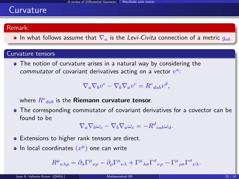
Remark:
In what follows assume that ∇a is the Levi-Civita connection of a metric gab
Curvature tensors
The notion of curvature arises in a natural way by considering thecommutator of covariant derivatives acting on a vector va:
∇a∇bvc −∇b∇avc = Rcdabvd,
where Rcdab is the Riemann curvature tensor.
The corresponding commutator of covariant derivatives for a covector can befound to be
∇a∇bωc −∇b∇aωc = −Rdcabωd.
Extensions to higher rank tensors are direct.
In local coordinates (xµ) one can write
Rµνλρ = ∂λΓµνρ − ∂ρΓµνλ + ΓµλσΓσνρ − ΓµρσΓσνλ.
Juan A. Valiente Kroon (QMUL) Mathematical GR 23 / 57
A review of Differential Geometry Manifolds with metric
Contractions and symmetries of the Riemann tensor
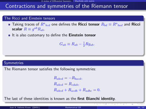
The Ricci and Einstein tensors
Taking traces of Rabcd one defines the Ricci tensor Rbd ≡ Rabad and Ricciscalar R ≡ gabRab.It is also customary to define the Einstein tensor
Gab ≡ Rab − 12Rgab.
Symmetries
The Riemann tensor satisfies the following symmetries:
Rabcd = −Rbacd,Rabcd = Rcdab,
Rabcd +Racdb +Radbc = 0.
The last of these identities is known as the first Bianchi identity.
Juan A. Valiente Kroon (QMUL) Mathematical GR 24 / 57
A review of Differential Geometry Manifolds with metric
Contractions and symmetries (II)
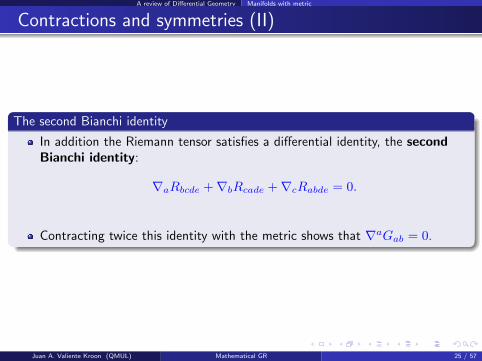
The second Bianchi identity
In addition the Riemann tensor satisfies a differential identity, the secondBianchi identity:
∇aRbcde +∇bRcade +∇cRabde = 0.
Contracting twice this identity with the metric shows that ∇aGab = 0.
Juan A. Valiente Kroon (QMUL) Mathematical GR 25 / 57
A brief survey of General Relativity
Outline
1 Outline of the course
2 A review of Differential GeometryBasic notionsManifolds with metric
3 A brief survey of General RelativityBasic notionsExact solutions
4 The Einstein equation as a wave equationThe scalar wave equationThe Maxwell equations as wave equationsThe Einstein equations in wave coordinates
Juan A. Valiente Kroon (QMUL) Mathematical GR 26 / 57
A brief survey of General Relativity Basic notions
Outline
1 Outline of the course
2 A review of Differential GeometryBasic notionsManifolds with metric
3 A brief survey of General RelativityBasic notionsExact solutions
4 The Einstein equation as a wave equationThe scalar wave equationThe Maxwell equations as wave equationsThe Einstein equations in wave coordinates
Juan A. Valiente Kroon (QMUL) Mathematical GR 27 / 57
A brief survey of General Relativity Basic notions
Introduction
Conceptual framework
General Relativity is a relativistic theory of gravity. It describes thegravitational interaction as a manifestation of the curvature of spacetime.
As it is the case of many other physical theories, General Relativity admits aformulation in terms of an initial value problem (Cauchy problem)whereby one prescribes the geometry of spacetime at some instant of timeand then one purports to reconstruct it from the initial data.
One has to make sense of what it means to prescribe the geometry ofspacetime at an instant of time.
Also how to reconstruct the spacetime from the data.
The initial value problem is the core of mathematical Relativity —an areaof active research with a number of interesting and challenging openproblems.
Juan A. Valiente Kroon (QMUL) Mathematical GR 28 / 57
A brief survey of General Relativity Basic notions
The Einstein field equations (I)
Basic objects:
General Relativity postulates the existence of a 4-dimensional manifold M,the spacetime manifold.
Point on M are called events.
M is endowed with a Lorentzian metric gab which in these lectures isassumed to have signature +2 —i.e. (−+ ++).
Spacetimes:
By a spacetime it will understood the a pair (M, gµν) where the metric gµνsatisfies the Einstein field equations
Rab − 12Rgab + λgab = Tab.
These equations show how matter and energy produce curvature of thespacetime.
λ denotes the so-called Cosmological constant.
Tab is the energy-momentum tensor of the matter model.
Juan A. Valiente Kroon (QMUL) Mathematical GR 29 / 57
A brief survey of General Relativity Basic notions
The Einstein field equations (II)
Conservation equations:
The conservation of energy-momentum is encoded in the condition
∇aTab = 0.
The conservation equation is consistent with the Einstein field equations as aconsequence of the second Bianchi identity:
∇a(Rab − 1
2Rgab + λgab)
= 0.
Test particles:
The geometry of the spacetime can be probed by means of the movement of testparticles:
massive test particles move along timelike geodesics;
rays of light move along null geodesics.
Juan A. Valiente Kroon (QMUL) Mathematical GR 30 / 57
A brief survey of General Relativity Basic notions
Isolated systems and the vacuum field equations
Some simplifying assumptions:
Attention will be restricted to the gravitational field of systems describingisolated bodies. Henceforth we assume that λ = 0.
Moreover, attention is restricted to the vacuum case for which Tab = 0. Thevacuum equations apply in the region external to an astrophysical source, butthey usefulness is not restricted to this.
One of the main properties of the gravitational field as described by GeneralRelativity is that it can be a source of itself —this is a manifestation of thenon-linearity of the Einstein field equations.
This property gives rise to a variety of phenomena that can be analysed bymeans of the so-called vacuum Einstein field equations without having toresort to any further considerations about matter sources:
Rab = 0.
The field equations prescribe the geometry of spacetime locally. However,they do not prescribe the topology of the spacetime manifold.
Juan A. Valiente Kroon (QMUL) Mathematical GR 31 / 57
A brief survey of General Relativity Exact solutions
Outline
1 Outline of the course
2 A review of Differential GeometryBasic notionsManifolds with metric
3 A brief survey of General RelativityBasic notionsExact solutions
4 The Einstein equation as a wave equationThe scalar wave equationThe Maxwell equations as wave equationsThe Einstein equations in wave coordinates
Juan A. Valiente Kroon (QMUL) Mathematical GR 32 / 57
A brief survey of General Relativity Exact solutions
Solutions to the Einstein field equations
Some conceptual questions:
Given the vacuum field equations a natural question is whether there are anysolutions.
What should one understand for a solution to the Einstein field equations?
Some first answers:
In first instance a solution is given by a metric gab expressed in a specificcoordinate system (xµ) —i.e. gµν . We call this an exact solution.
Exact solutions are our main way of acquiring intuition about the behaviourof generic solutions to the Einstein field equations.
Juan A. Valiente Kroon (QMUL) Mathematical GR 33 / 57
A brief survey of General Relativity Exact solutions
The Minkowski spacetime
In a nutshell:
The solution is encoded in the line element
g = ηµνdxµdxν , ηµν = diag(−1, 1, 1, 1).
One clearly verifies that for this metric in these coordinates Rµνλρ = 0 sothat Rµν = 0.
As Rµν are the components of a tensor in a specific coordinate system oneconcludes then Rab = 0.
Any metric related to by a coordinate transformation is a solution to thevacuum field equations.
Observation:
The example in the previous paragraph shows that as a consequence of thetensorial character of the Einstein field equations a solution to the equations is, infact, an equivalence class of solutions related to each other by means ofcoordinate transformations.
Juan A. Valiente Kroon (QMUL) Mathematical GR 34 / 57
A brief survey of General Relativity Exact solutions
Symmetry assumptions
Motivation:
In order to find further explicit solutions to the field equations one needs tomake some sort of assumptions about the spacetime.
A standard assumption is that the spacetime has continuous symmetries.
Continuous symmetries and Killing vectors
The notion of a continuous symmetry is formalised by the notion of adiffeomorphism.
A diffeomorphism is a smooth map φ of M onto itself.
Intuitively the diffeomorphism moves the points in the manifold along curvesin the manifold —the orbits of the symmetry.
Let ξa denote the tangent vector to the orbits. The mapping φ is called anisometry if Lξgab = 0. It can be checked that
∇aξb +∇bξa = 0.
This equation is called the Killing equation.
Juan A. Valiente Kroon (QMUL) Mathematical GR 35 / 57
A brief survey of General Relativity Exact solutions
Properties of the Killing equation:
Restrictions on the spacetime
The Killing equation is overdetermined —i.e. it does not admit a solutionfor a general spacetime.
Thus a solution, if exists, imposes restrictions on the spacetime.
Using the commutator
∇a∇bξc −∇b∇aξc = −Rdcabξd,
together with the Killing equation one obtains
∇a∇bξc = Rdabcξd.
This is an integrability condition for the Killing equation —i.e. a necessarycondition that needs to be satisfied by any solution.
Juan A. Valiente Kroon (QMUL) Mathematical GR 36 / 57
A brief survey of General Relativity Exact solutions
Spherical symmetry
Spherical symmetry in a nutshell:
An important type of symmetry is given by the so-called sphericalsymmetry.
There exists a 3-dimensional group of symmetries with 2-dimensionalspacelike orbits.
Each orbit is an homogeneous and isotropic manifold.
The orbits are required to be compact and to have constant positivecurvature.
Juan A. Valiente Kroon (QMUL) Mathematical GR 37 / 57
A brief survey of General Relativity Exact solutions
The Schwarzschild spacetime
The metric in standard coordinates:
In standard coordinates (t, r, θ, ϕ) by the expression
g = −Å
1− 2m
r
ãdt2 +
Å1− 2m
r
ã−1
dr2 + r2(dθ2 + sin2 θdϕ2).
This solution is spherically symmetric and static —i.e. time independent.
The Schwarzschild solution is of particular interest as it gives the simplestexample of a black hole. The spacetime manifold can be explicitly verified tobe singular at r = 0. This singularity is hidden behind a horizon.
Juan A. Valiente Kroon (QMUL) Mathematical GR 38 / 57
A brief survey of General Relativity Exact solutions
Properties of the Schwarzschild spacetime
Rigidity results:
The Schwarzschild spacetime satisfies a number of rigidity properties —i.e.certain properties about solutions to the Einstein field equations immediatelyimply other properties.
Staticity can be obtained from the assumption of spherical symmetry —theBirkhoff theorem: any spherically symmetric solution to the vacuum fieldequations is locally isometric to the Schwarzschild solution
The Schwarzschild solution can be characterised as the only static solution ofthe vacuum field equations satisfying a certain (reasonable) behaviour atinfinity —asymptotic flatness: the requirement that asymptotically, themetric behaves like the Minkowski metric. This result is known as theno-hair theorem.
Juan A. Valiente Kroon (QMUL) Mathematical GR 39 / 57
A brief survey of General Relativity Exact solutions
Other exact solutions (I)
The Kerr spacetime:
In order to obtain more exact solutions reduce the number of symmetries—accordingly the task of finding solutions becomes harder.
A natural assumption is to look for axially symmetric and stationarysolutions.
stationarity is a form of time independence which is compatible with thenotion of rotation —to be seen in more detail.
The above assumptions lead to the Kerr spacetime describing a timeindependent rotating black hole.
Juan A. Valiente Kroon (QMUL) Mathematical GR 40 / 57
A brief survey of General Relativity Exact solutions
Other exact solutions (II)
Surveys of exact solutions:
Although there are a huge number of explicit solutions to the Einstein fieldequation —see e.g. [Stephani et al], the number of solutions with aphysical/geometric relevance is much more restricted.
For a discussion of some of the physically/geometrically important solutionssee e.g. [Griffiths & Podolski].
For exact solutions describing isolated systems which are time dependent,there are no known solutions without some sort of pathology.
Juan A. Valiente Kroon (QMUL) Mathematical GR 41 / 57
A brief survey of General Relativity Exact solutions
Abstract analysis of the Einstein field equations
An alternative to exact solutions:
Use the general features and structure of the equations to assert existence inan abstract sense.
Proceed in the same way to establish uniqueness and other properties of thesolutions.
In this way can explore more systematically the space of solutions to thetheory.
After this of analysis has been carried out one can proceed to constructsolutions numerically.
Juan A. Valiente Kroon (QMUL) Mathematical GR 42 / 57
The Einstein equation as a wave equation
Outline
1 Outline of the course
2 A review of Differential GeometryBasic notionsManifolds with metric
3 A brief survey of General RelativityBasic notionsExact solutions
4 The Einstein equation as a wave equationThe scalar wave equationThe Maxwell equations as wave equationsThe Einstein equations in wave coordinates
Juan A. Valiente Kroon (QMUL) Mathematical GR 43 / 57
The Einstein equation as a wave equation
Introduction:
A strategy:
A strategy to study generic solutions to the Einstein field equations is toformulate an initial value problem (Cauchy problem) for the Einstein fieldequations.
In order to do so, one needs to bring the equations to some standard form inwhich the methods of the theory of partial differential equations can beapplied.
One expects the Einstein equations to imply some evolution process.
Suitable equations describing evolutive processess are wave equations.
Juan A. Valiente Kroon (QMUL) Mathematical GR 44 / 57
The Einstein equation as a wave equation The scalar wave equation
Outline
1 Outline of the course
2 A review of Differential GeometryBasic notionsManifolds with metric
3 A brief survey of General RelativityBasic notionsExact solutions
4 The Einstein equation as a wave equationThe scalar wave equationThe Maxwell equations as wave equationsThe Einstein equations in wave coordinates
Juan A. Valiente Kroon (QMUL) Mathematical GR 45 / 57
The Einstein equation as a wave equation The scalar wave equation
The scalar wave equation (I)
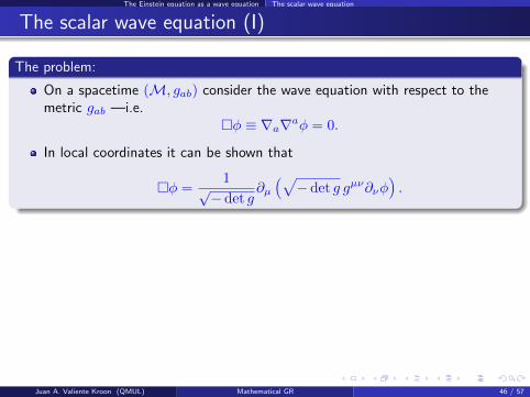
The problem:
On a spacetime (M, gab) consider the wave equation with respect to themetric gab —i.e.
�φ ≡ ∇a∇aφ = 0.
In local coordinates it can be shown that
�φ =1√− det g
∂µÄ√− det g gµν∂νφ
ä.
Principal part:
The principal part of the equation corresponds to the terms containing thehighest order derivatives of the scalar field φ:
gµν∂µ∂νφ.
The structure in this expression is particular of a class of partial differentialequations known as hyperbolic equations.
Juan A. Valiente Kroon (QMUL) Mathematical GR 46 / 57
The Einstein equation as a wave equation The scalar wave equation
The scalar wave equation (I)
The problem:
On a spacetime (M, gab) consider the wave equation with respect to themetric gab —i.e.
�φ ≡ ∇a∇aφ = 0.
In local coordinates it can be shown that
�φ =1√− det g
∂µÄ√− det g gµν∂νφ
ä.
Principal part:
The principal part of the equation corresponds to the terms containing thehighest order derivatives of the scalar field φ:
gµν∂µ∂νφ.
The structure in this expression is particular of a class of partial differentialequations known as hyperbolic equations.
Juan A. Valiente Kroon (QMUL) Mathematical GR 46 / 57
The Einstein equation as a wave equation The scalar wave equation
The scalar wave equation (II)
The scalar wave in Minkowski spacetime
The most well known hyperbolic equation is the wave equation on theMinkowski spacetime.
In standard Cartesian coordinates one has that
�φ = ηµν∂µ∂νφ = ∂2xφ+ ∂2y + ∂2zφ− ∂2t φ = 0.
Cauchy problem for the wave equation
The Cauchy problem for the wave equations and more generally hyperbolicequations is well understood at least in a local setting.
If one prescribes the field φ and its derivative ∂µφ at some fiduciary instantof time t = 0, then the equation �φ = 0 has a solution for suitably smalltimes (local existence).
This solution is unique in its existence interval and it has continuousdependence on the initial data.
The solution exhibits finite speed propagation.
Juan A. Valiente Kroon (QMUL) Mathematical GR 47 / 57
The Einstein equation as a wave equation The Maxwell equations as wave equations
Outline
1 Outline of the course
2 A review of Differential GeometryBasic notionsManifolds with metric
3 A brief survey of General RelativityBasic notionsExact solutions
4 The Einstein equation as a wave equationThe scalar wave equationThe Maxwell equations as wave equationsThe Einstein equations in wave coordinates
Juan A. Valiente Kroon (QMUL) Mathematical GR 48 / 57
The Einstein equation as a wave equation The Maxwell equations as wave equations
The Maxwell equations (I)
The source free equations:
A useful model to discuss certain issues arising in the Einstein field equationsare the source-free Maxwell equations:
∇aFab = 0, ∇[aFbc] = 0,
where Fab = −Fab is the Faraday tensor.
A solution to the second Maxwell equation is given by
Fab = ∇aAb −∇bAa,
where Aa is the so-called gauge potential.
Gauge freedom:
The gauge potential does not determine the the Faraday tensor in a uniqueway as Aa +∇aφ with φ as scalar field gives the same Fab.
Juan A. Valiente Kroon (QMUL) Mathematical GR 49 / 57
The Einstein equation as a wave equation The Maxwell equations as wave equations
The Maxwell equations (II)
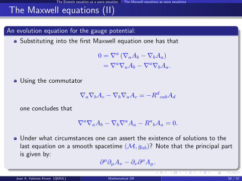
An evolution equation for the gauge potential:
Substituting into the first Maxwell equation one has that
0 = ∇a (∇aAb −∇bAa)
= ∇a∇aAb −∇a∇bAa.
Using the commutator
∇a∇bAc −∇b∇aAc = −RdcabAd
one concludes that
∇a∇aAb −∇b∇aAa −RabAa = 0.
Under what circumstances one can assert the existence of solutions to thelast equation on a smooth spacetime (M, gab)? Note that the principal partis given by:
∂µ∂µAν − ∂ν∂µAµ.
Juan A. Valiente Kroon (QMUL) Mathematical GR 50 / 57
The Einstein equation as a wave equation The Maxwell equations as wave equations
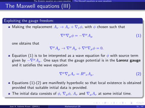
The Maxwell equations (III)
Exploiting the gauge freedom:
Making the replacement Aν → Aν +∇νφ, with φ chosen such that
∇µ∇µφ = −∇µAµ (1)
one obtains that∇µAµ → ∇µAµ +∇µ∇µφ = 0.
Equation (1) is to be interpreted as a wave equation for φ with source termgiven by −∇µAµ. One says that the gauge potential is in the Lorenz gaugeand it satisfies the wave equation
∇µ∇µAν = RµνAµ. (2)
Equations (1)-(2) are manifestly hyperbolic so that local existence is obtainedprovided that suitable initial data is provided.
The initial data consists of φ, ∇µφ, Aν and ∇µAν at some initial time.
Juan A. Valiente Kroon (QMUL) Mathematical GR 51 / 57
The Einstein equation as a wave equation The Einstein equations in wave coordinates
Outline
1 Outline of the course
2 A review of Differential GeometryBasic notionsManifolds with metric
3 A brief survey of General RelativityBasic notionsExact solutions
4 The Einstein equation as a wave equationThe scalar wave equationThe Maxwell equations as wave equationsThe Einstein equations in wave coordinates
Juan A. Valiente Kroon (QMUL) Mathematical GR 52 / 57
The Einstein equation as a wave equation The Einstein equations in wave coordinates
The Einstein equations (I)
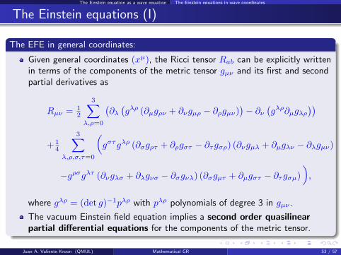
The EFE in general coordinates:
Given general coordinates (xµ), the Ricci tensor Rab can be explicitly writtenin terms of the components of the metric tensor gµν and its first and secondpartial derivatives as
Rµν = 12
3∑λ,ρ=0
(∂λ(gλρ (∂µgρν + ∂νgµρ − ∂ρgµν)
)− ∂ν
(gλρ∂µgλρ
))+ 1
4
3∑λ,ρ,σ,τ=0
Ågστgλρ (∂σgρτ + ∂ρgστ − ∂τgσρ) (∂νgµλ + ∂µgλν − ∂λgµν)
−gρσgλτ (∂νgλσ + ∂λgνσ − ∂σgνλ) (∂σgµτ + ∂µgστ − ∂τgσµ)
ã,
where gλρ = (det g)−1pλρ with pλρ polynomials of degree 3 in gµν .
The vacuum Einstein field equation implies a second order quasilinearpartial differential equations for the components of the metric tensor.
Juan A. Valiente Kroon (QMUL) Mathematical GR 53 / 57
The Einstein equation as a wave equation The Einstein equations in wave coordinates
The Einstein equations (II)
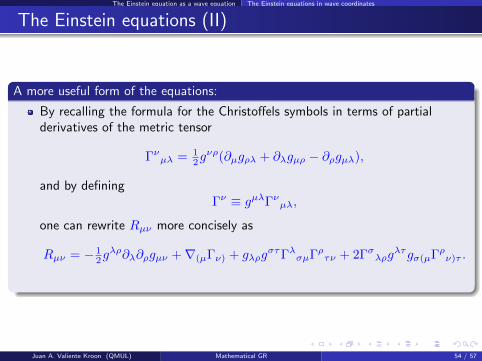
A more useful form of the equations:
By recalling the formula for the Christoffels symbols in terms of partialderivatives of the metric tensor
Γνµλ = 12gνρ(∂µgρλ + ∂λgµρ − ∂ρgµλ),
and by definingΓν ≡ gµλΓνµλ,
one can rewrite Rµν more concisely as
Rµν = − 12gλρ∂λ∂ρgµν +∇(µΓν) + gλρg
στΓλσµΓρτν + 2Γσλρgλτgσ(µΓρν)τ .
Juan A. Valiente Kroon (QMUL) Mathematical GR 54 / 57
The Einstein equation as a wave equation The Einstein equations in wave coordinates
The Einstein equations (II)
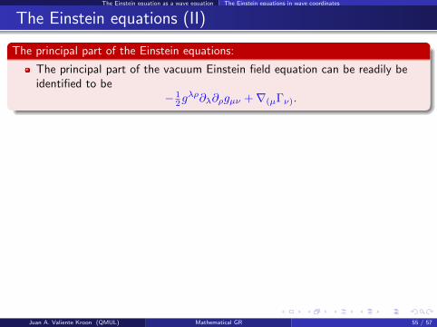
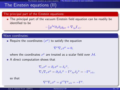
The principal part of the Einstein equations:
The principal part of the vacuum Einstein field equation can be readily beidentified to be
− 12gλρ∂λ∂ρgµν +∇(µΓν).
Wave coordinates:
Require the coordinates (xµ) to satisfy the equation
∇ν∇νxµ = 0,
where the coordinates xµ are treated as a scalar field over M.
A direct computation shows that
∇νxµ = ∂νxµ = δν
µ,
∇λ∇νxµ = ∂λδνµ − Γρλνδρ
µ = −Γµνλ,
so that∇ν∇νxµ = gνλΓµνλ = −Γµ.
Juan A. Valiente Kroon (QMUL) Mathematical GR 55 / 57
The Einstein equation as a wave equation The Einstein equations in wave coordinates
The Einstein equations (II)
The principal part of the Einstein equations:
The principal part of the vacuum Einstein field equation can be readily beidentified to be
− 12gλρ∂λ∂ρgµν +∇(µΓν).
Wave coordinates:
Require the coordinates (xµ) to satisfy the equation
∇ν∇νxµ = 0,
where the coordinates xµ are treated as a scalar field over M.
A direct computation shows that
∇νxµ = ∂νxµ = δν
µ,
∇λ∇νxµ = ∂λδνµ − Γρλνδρ
µ = −Γµνλ,
so that∇ν∇νxµ = gνλΓµνλ = −Γµ.
Juan A. Valiente Kroon (QMUL) Mathematical GR 55 / 57
The Einstein equation as a wave equation The Einstein equations in wave coordinates
The Einstein equations (III)
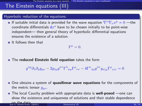
Hyperbolic reduction of the equations:
If suitable initial data is provided for the wave equation ∇ν∇νxµ = 0 —thecoordinate differentials dxa have to be chosen initially to be point-wiseindependent— then general theory of hyperbolic differential equationsensures the existence of a solution.
It follows then thatΓµ = 0.
The reduced Einstein field equation takes the form
gλρ∂λ∂ρgµν − 2gλρgστΓλσµΓρτν − 4Γσλρg
λτgσ(µΓρν)τ = 0
One obtains a system of quasilinear wave equations for the components ofthe metric tensor gµν .
The local Cauchy problem with appropriate data is well-posed —one canshow the existence and uniqueness of solutions and their stable dependenceon the data.
Juan A. Valiente Kroon (QMUL) Mathematical GR 56 / 57
The Einstein equation as a wave equation The Einstein equations in wave coordinates
The Einstein equations (IV)
Some remarks:
The system of equations is called the reduced Einstein field equations andthe procedure a hyperbolic reduction.
For the reduced equation one readily has a developed theory of existence anduniqueness available.
The introduction of a specific system of coordinates breaks the tensorialcharacter of the Einstein field equations.
Given a solution to the reduced Einstein field equations, the latter will alsoimply a solution to the actual EFE as long as (xµ) satisfy the equation∇ν∇νxµ = 0. This requires some delicate analysis —to be seen later.
The domain on which the coordinates (xµ) form a good coordinate systemdepends on the initial data prescribed and the solution gµν itself. There islittle that can be said a priori about the domain of existence of thecoordinates.
The data for the reduced equation consists of a prescription of gµν and ∂λgµνat some initial time t = 0. The next step in our discussion is tounderstand the meaning of this data.
Juan A. Valiente Kroon (QMUL) Mathematical GR 57 / 57