Embed Size (px)
Citation preview

BULLETIN (New Series) OF THEAMERICAN MATHEMATICAL SOCIETYVolume 47, Number 4, October 2010, Pages 567–638S 0273-0979(2010)01304-5Article electronically published on July 30, 2010
MATHEMATICAL GENERAL RELATIVITY: A SAMPLER
PIOTR T. CHRUSCIEL, GREGORY J. GALLOWAY, AND DANIEL POLLACK
Abstract. We provide an introduction to selected recent advances in themathematical understanding of Einstein’s theory of gravitation.
Contents
1. Introduction 5682. Elements of Lorentzian geometry and causal theory 5692.1. Lorentzian manifolds 5692.2. Einstein equations 5712.3. Elements of causal theory 5712.3.1. Pasts and futures 5722.3.2. Causality conditions 5732.3.3. Domains of dependence 5752.4. Submanifolds 5763. Stationary black holes 5773.1. The Schwarzschild metric 5773.2. Rotating black holes 5793.3. Killing horizons 5803.3.1. Surface gravity 5813.3.2. Average surface gravity 5823.4. Asymptotically flat metrics 5823.5. Asymptotically flat stationary metrics 5833.6. Domains of outer communications, event horizons 5833.7. Uniqueness theorems 5844. The Cauchy problem 5864.1. The local evolution problem 5874.1.1. Wave-coordinates 5874.2. Cauchy data 5894.3. Solutions global in space 5905. Initial data sets 5925.1. The constraint equations 5925.2. Mass inequalities 5955.2.1. The Positive Mass Theorem 595
Received by the editors September 11, 2008 and, in revised form, November 6, 2008.2010 Mathematics Subject Classification. Primary 83-02.Support by the Banff International Research Station (Banff, Canada), and by Institut Mittag-
Leffler (Djursholm, Sweden) is gratefully acknowledged. The research of the second author hasbeen supported in part by an NSF grant DMS 0708048.
c©2010 American Mathematical SocietyReverts to public domain 28 years from publication
567

568 PIOTR T. CHRUSCIEL, GREGORY J. GALLOWAY, AND DANIEL POLLACK
5.2.2. Riemannian Penrose Inequality 5965.2.3. Quasi-local mass 5975.3. Applications of gluing techniques 5975.3.1. The linearized constraint equations and KIDs 5975.3.2. Corvino’s result 5985.3.3. Conformal gluing 5995.3.4. Initial data engineering 6006. Evolution 6016.1. Strong cosmic censorship 6016.1.1. Gowdy toroidal metrics 6036.1.2. Other U(1)× U(1)-symmetric models 6046.1.3. Spherical symmetry 6046.2. Weak cosmic censorship 6056.3. Stability of vacuum cosmological models 6066.3.1. U(1) symmetry 6066.3.2. Future stability of hyperbolic models 6076.4. Stability of Minkowski space-time 6076.4.1. The Christodoulou–Klainerman proof 6076.4.2. The Lindblad–Rodnianski proof 6086.5. Toward stability of Kerr: Wave equations on black hole backgrounds 6106.6. Bianchi A metrics 6106.7. The mixmaster conjecture 6137. Marginally trapped surfaces 6157.1. Null hypersurfaces 6157.2. Trapped and marginally trapped surfaces 6177.3. Stability of MOTSs 6207.4. On the topology of black holes 6217.5. Existence of MOTSs 623Appendix A. Open problems 625Acknowledgments 627About the authors 627References 627
1. Introduction
Mathematical general relativity is, by now, a well-established vibrant branch ofmathematics. It ties fundamental problems of gravitational physics with beautifulquestions in mathematics. The object is the study of manifolds equipped with aLorentzian metric satisfying the Einstein field equations. Some highlights of its his-tory include the discovery by Choquet-Bruhat of a well-posed Cauchy problem [140],subsequently globalized by Choquet-Bruhat and Geroch [75], the singularity the-orems of Penrose and Hawking [151, 238], the proof of the positive mass theoremby Schoen and Yau [257], and the proof of stability of Minkowski space-time byChristodoulou and Klainerman [88].
There has recently been spectacular progress in the field on many fronts, includ-ing the Cauchy problem, stability, cosmic censorship, construction of initial data,

MATHEMATICAL GENERAL RELATIVITY 569
and asymptotic behaviour, many of which will be described here. Mutual bene-fits are drawn, and progress is being made, from the interaction between generalrelativity and geometric analysis and the theory of elliptic and hyperbolic partialdifferential equations. The Einstein equation shares issues of convergence, collapse,and stability with other important geometric PDEs, such as the Ricci flow and themean curvature flow. A steadily growing overlap between the relevant scientificcommunities can be seen. For all these reasons it appeared timely to provide amathematically oriented reader with an introductory survey of the field. This isthe purpose of the current work.
In Section 2 we survey the Lorentzian causality theory, the basic language for de-scribing the structure of space-times. In Section 3 the reader is introduced to blackholes, perhaps the most fascinating prediction of Einstein’s theory of gravitation,and the source of many deep (solved or unsolved) mathematical problems. In Sec-tion 4 the Cauchy problem for the Einstein equations is considered, laying down thefoundations for a systematic construction of general space-times. Section 5 exam-ines initial data sets, as needed for the Cauchy problem, and their global properties.In Section 6 we discuss the dynamics of the Einstein equations, including questionsof stability and predictability; the latter question is known under the baroque nameof “strong cosmic censorship”. Section 7 deals with trapped and marginally trappedsurfaces, which signal the presence of black holes and have tantalizing connectionswith classical minimal surface theory. The paper is sprinkled with open problems,which are collected in Appendix A.
2. Elements of Lorentzian geometry and causal theory
2.1. Lorentzian manifolds. In general relativity, and related theories, the spaceof physical events is represented by a Lorentzian manifold. A Lorentzian manifoldis a smooth (Hausdorff, paracompact) manifold M = M n+1 of dimension n + 1,equipped with a Lorentzian metric g. A Lorentzian metric is a smooth assignmentto each point p ∈ M of a symmetric, nondegenerate bilinear form on the tangentspace TpM of signature (− + · · ·+). Hence, if {e0, e1, . . . , en} is an orthonormalbasis for TpM with respect to g, then, perhaps after reordering the basis, the matrix[g(ei, ej)] equals diag (−1,+1, . . . ,+1). A vector v =
∑vαeα then has square norm,
(2.1) g(v, v) = −(v0)2 +∑
(vi)2 ,
which can be positive, negative or zero. This leads to the causal character of vectors,and indeed to the causal theory of Lorentzian manifolds, which we shall discuss inSection 2.3.
On a coordinate neighborhood (U, xα)= (U, x0, x1, . . . , xn), the metric g is com-pletely determined by its metric component functions on U , gαβ := g( ∂
∂xα ,∂
∂xβ ),
0 ≤ α, β ≤ n: For v = vα ∂∂xα , w = wβ ∂
∂xβ ∈ TpM , p ∈ U , g(v, w) = gαβvαwβ .
(Here we have used the Einstein summation convention: if, in a coordinate chart, anindex appears repeated, once up and once down, then summation over that indexis implied.) Classically the metric in coordinates is displayed via the line element,ds2 = gαβdx
αdxβ .The prototype Lorentzian manifold is Minkowski space R
1,n, the space-time ofspecial relativity. This is R
n+1, equipped with the Minkowski metric, which, withrespect to Cartesian coordinates (x0, x1, . . . , xn), is given by
ds2 = −(dx0)2 + (dx1)2 + · · ·+ (dxn)2 .

570 PIOTR T. CHRUSCIEL, GREGORY J. GALLOWAY, AND DANIEL POLLACK
Each tangent space of a Lorentzian manifold is isometric to Minkowski space, andin this way the local accuracy of special relativity is built into general relativity.
Every Lorentzian manifold (or, more generally, pseudo-Riemannian manifold)(M n+1, g) comes equipped with a Levi-Civita connection (or covariant differentia-tion operator) ∇ that enables one to compute the directional derivative of vectorfields. Hence, for smooth vector fields X,Y ∈ X(M ), ∇XY ∈ X(M ) denotes the co-variant derivative of Y in the direction X. The Levi-Civita connection is the uniqueconnection ∇ on (M n+1, g) that is (i) symmetric (or torsion free), i.e., that satisfies∇XY −∇Y X = [X,Y ] for all X,Y ∈ X(M), and (ii) compatible with the metric,i.e. that obeys the metric product rule, X(g(Y, Z)) = g(∇XY, Z) + g(Y,∇XZ), forall X,Y, Z ∈ X(M).
In a coordinate chart (U, xα) one has
(2.2) ∇XY = (X(Y μ) + ΓμαβX
αY β)∂μ ,
where Xα, Y α are the components of X and Y , respectively, with respect to thecoordinate basis ∂α = ∂
∂xα , and where the Γμαβ ’s are the classical Christoffel symbols
given in terms of the metric components by
(2.3) Γμαβ =
1
2gμν(∂βgαν + ∂αgβν − ∂νgαβ) .
Note that the coordinate expression (2.2) can also be written as
(2.4) ∇XY = Xα∇αYμ∂μ ,
where ∇αYμ (often written classically as Y μ
;α) is given by
(2.5) ∇αYμ = ∂αY
μ + ΓμαβY
β .
We shall feel free to interchange between coordinate and coordinate-free notation.The Levi-Civita connection∇ extends in a natural way to a covariant differentiationoperator on all tensor fields.
The Riemann curvature tensor of (M n+1, g) is the map R : X(M) × X(M) ×X(M) → X(M), (X,Y, Z) → R(X,Y )Z, given by
(2.6) R(X,Y )Z = ∇X∇Y Z −∇Y ∇XZ −∇[X,Y ]Z .
This expression is linear in X,Y, Z ∈ X(M ) with respect to C∞(M ). This impliesthat R is indeed tensorial, i.e., that the value of R(X,Y )Z at p ∈ M depends onlyon the value of X,Y, Z at p.
Equation (2.6) shows that the Riemann curvature tensor measures the extentto which covariant differentiation fails to commute. This failure to commute maybe seen as an obstruction to the existence of parallel vector fields. By Riemann’stheorem, a Lorentzian manifold is locally Minkowskian if and only if the Riemanncurvature tensor vanishes.
The components Rμγαβ of the Riemann curvature tensor R in a coordinate chart
(U, xα) are determined by the equations R(∂α, ∂β)∂γ = Rμγαβ∂μ. Equations (2.2)
and (2.6) then yield the following explicit formula for the curvature components interms of the Christoffel symbols:
(2.7) Rμγαβ = ∂αΓ
μγβ − ∂βΓ
μγα + Γν
γβΓμνα − Γν
γαΓμνβ .
The Ricci tensor, Ric, is a bilinear form obtained by contraction of the Riemanncurvature tensor, i.e., its components Rμν = Ric(∂μ, ∂ν) are determined by tracing,Rμν = Rα
μαν . Symmetries of the Riemann curvature tensor imply that the Ricci

MATHEMATICAL GENERAL RELATIVITY 571
tensor is symmetric, Rμν = Rνμ. By tracing the Ricci tensor, we obtain the scalarcurvature R = gμνRμν , where gμν denotes the matrix inverse to gμν .
2.2. Einstein equations. The Einstein equation (with cosmological constant Λ),the field equation of general relativity, is the tensor equation
(2.8) Ric− 1
2Rg + Λg = 8πT ,
where T is the energy-momentum tensor (see, e.g., Section 6.4.2 for an example ofan energy-momentum tensor). When expressed in terms of coordinates, the Einsteinequation becomes a system of second-order equations for the metric components gμνand the nongravitational field variables introduced through the energy-momentumtensor. We say that space-time obeys the vacuum Einstein equation if it obeys theEinstein equation with T = 0.
The Riemann curvature tensor has a number of symmetry properties, one ofwhich is the so-called first Bianchi identity:
Rαβγδ +Rαγδβ +Rαδβγ = 0 .
The curvature tensor also obeys a differential identity known as the second Bianchiidentity:
(2.9) ∇σRαβγδ +∇αRβσγδ +∇βRσαγδ = 0 .
When twice contracted, (2.9) yields the following divergence identity:
(2.10) ∇α
(
Rαβ − R
2gαβ
)
= 0 .
This plays a fundamental role in general relativity, as, in particular, it implies, inconjunction with the Einstein equation, local conservation of energy, ∇αT
αβ = 0. Italso plays an important role in the mathematical analysis of the Einstein equations;see Section 4 for further discussion.
2.3. Elements of causal theory. Many concepts and results in general relativitymake use of the causal theory of Lorentzian manifolds. The starting point for causaltheory is the causal classification of tangent vectors. Let (M n+1, g) be a Lorentzianmanifold. A vector v ∈ TpM is timelike (resp., spacelike, null) provided g(v, v) < 0(resp., g(v, v) > 0, g(v, v) = 0). The collection of null vectors forms a double coneVp in TpM (recall (2.1)), called the null cone at p; see Figure 2.1.
The timelike vectors at p point inside the null cone and the spacelike vectorspoint outside. We say that v ∈ TpM is causal if it is timelike or null. We define the
length of causal vectors as |v| =√−g(v, v). Causal vectors v, w ∈ TpM that point
into the same half-cone of the null cone Vp obey the reverse triangle inequality,|v + w| ≥ |v|+ |w|. Geometrically, this is the source of the twin paradox.
These notions of causality extend to curves. Let γ : I → M , t → γ(t), be asmooth curve in M , then γ is said to be timelike (resp., spacelike, null, causal)provided each of its velocity vectors γ′(t) is timelike (resp., spacelike, null, causal).Heuristically, in accordance with relativity, information flows along causal curves,and so such curves are the focus of attention in causal theory. The notion of acausal curve extends in a natural way to piecewise smooth curves, and we willnormally work within this class. As usual, we define a geodesic to be a curvet → γ(t) of zero covariant acceleration, ∇γ′γ′ = 0. Since geodesics γ are constant

572 PIOTR T. CHRUSCIEL, GREGORY J. GALLOWAY, AND DANIEL POLLACK
p
future pointing timelike
past pointing timelike
future pointing nullpast pointing null
Figure 2.1. The light cone at p.
speed curves (g(γ′, γ′) = const.), each geodesic in a Lorentzian manifold is eithertimelike, spacelike or null.
The length of a causal curve γ : [a, b] → M is defined as
L(γ) = Length of γ =
∫ b
a
|γ′(t)|dt =∫ b
a
√−g(γ′(t), γ′(t)) dt .
If γ is timelike, one can introduce an arc length parameter along γ. In generalrelativity, a timelike curve corresponds to the history of an observer, and the arclength parameter, called proper time, corresponds to time kept by the observer.Using the existence and properties of geodesically convex neighborhoods [232] onecan show that causal geodesics are locally maximal (i.e., locally longest amongcausal curves).
Each null cone Vp consists of two half-cones, one of which may designated asthe future cone and the other as the past cone at p. If the assignment of a pastand future cone at each point of M can be carried out in a continuous mannerover M , then M is said to be time-orientable. There are various ways to makethe phrase “continuous assignment” precise, but they all result in the followingfact: a Lorentzian manifold (M n+1, g) is time-orientable if and only if it admitsa smooth timelike vector field Z. If M is time-orientable, the choice of a smoothtimelike vector field Z fixes a time orientation on M : For any p ∈ M , a causalvector v ∈ TpM is future directed (resp. past directed) provided g(v, Z) < 0 (resp.g(v, Z) > 0). Thus, v is future directed if it points into the same null half-coneat p as Z. We note that a Lorentzian manifold that is not time-orientable alwaysadmits a double cover that is. By a space-time we mean a connected time-orientedLorentzian manifold (M n+1, g). Henceforth, we restrict our attention to space-times.
2.3.1. Pasts and futures. Let (M , g) be a space-time. A timelike (resp. causal)curve γ : I → M is said to be future directed provided each tangent vector γ′(t),t ∈ I, is future directed. (Past-directed timelike and causal curves are defined in atime-dual manner.) I+(p), the timelike future of p ∈ M , is the set consisting ofall points q ∈ M for which there exists a future-directed timelike curve from p toq. J+(p), the causal future of p ∈ M , is the set consisting of p and all points q forwhich there exists a future-directed causal curve from p to q. In Minkowski space

MATHEMATICAL GENERAL RELATIVITY 573
R1,n these sets have a simple structure: For each p ∈ R
1,n, ∂I+(p) = J+(p) \ I+(p)is the future cone at p generated by the future-directed null rays emanating fromp. I+(p) consists of the points inside the cone, and J+(p) consists of the pointson and inside the cone. In general, the curvature and topology of space-time canstrongly influence the structure of these sets.
Since a timelike curve remains timelike under small smooth perturbations, it isheuristically clear that the sets I+(p) are in general open; a careful proof makes useof properties of geodesically convex sets. On the other hand, the sets J+(p) neednot be closed in general, as can be seen by considering the space-time obtained byremoving a point from Minkowski space.
It follows from variational arguments that, for example, if q ∈ I+(p) and r ∈J+(q), then r ∈ I+(p). This and related claims are in fact a consequence of thefollowing fundamental causality result [232].
Proposition 2.1. If q ∈ J+(p)\ I+(p), i.e., if q is in the causal future of p but notin the timelike future of p, then any future-directed causal curve from p to q mustbe a null geodesic.
Given a subset S ⊂ M , I+(S), the timelike future of S, consists of all pointsq ∈ M for which there exists a future-directed timelike curve from a point in S toq. J+(S), the causal future of S, consists of the points of S and all points q ∈ Mfor which there exists a future-directed causal curve from a point in S to q. Notethat I+(S) =
⋃p∈S I+(p). Hence, as a union of open sets, I+(S) is always open.
The timelike and causal pasts I−(p), J−(p), I−(S), J−(S) are defined in a time-dual manner in terms of past-directed timelike and causal curves. It is sometimesconvenient to consider pasts and futures within some open subset U of M . Forexample, I+(p, U) denotes the set consisting of all points q ∈ U for which thereexists a future-directed timelike curve from p to q contained in U .
Sets of the form ∂I±(S) are called achronal boundaries and have nice structuralproperties: they are achronal Lipschitz hypersurfaces, ruled, in a certain sense, bynull geodesics [232]. (A set is achronal if no two of its points can be joined by atimelike curve.)
2.3.2. Causality conditions. A number of results in Lorentzian geometry and gen-eral relativity require some sort of causality condition. It is perhaps natural onphysical grounds to rule out the occurrence of closed timelike curves. Physically,the existence of such a curve signifies the existence of an observer who is able totravel into his/her own past, which leads to a variety of paradoxical situations.A space-time M satisfies the chronology condition provided there are no closedtimelike curves in M . It can be shown that all compact space-times violate thechronology condition, and for this reason compact space-times have been of limitedinterest in general relativity.
A somewhat stronger condition than the chronology condition is the causalitycondition. A space-time M satisfies the causality condition provided there areno closed (nontrivial) causal curves in M . A slight weakness of this condition isthat there are space-times which satisfy the causality condition, but contain causalcurves that are almost closed ; see, e.g., [154, p. 193].
It is useful to have a condition that rules out almost closed causal curves. Aspace-time M is said to be strongly causal at p ∈ M provided there are arbitrarilysmall neighborhoods U of p such that any causal curve γ which starts in and leaves

574 PIOTR T. CHRUSCIEL, GREGORY J. GALLOWAY, AND DANIEL POLLACK
U never returns to U . M is strongly causal if it is strongly causal at each ofits points. Thus, heuristically speaking, M is strongly causal provided there areno closed or almost closed causal curves in M . Strong causality is the standardcausality condition of space-time geometry, and although there are even strongercausality conditions, it is sufficient for most applications. A very useful fact aboutstrongly causal space-times is the following: If M is strongly causal, then any future(or past) inextendible causal curve γ cannot be imprisoned or partially imprisonedin a compact set. That is to say, if γ starts in a compact set K, it must eventuallyleave K for good.
We now come to a fundamental condition in space-time geometry, that of globalhyperbolicity. Mathematically, global hyperbolicity is a basic niceness conditionthat often plays a role analogous to geodesic completeness in Riemannian geom-etry. Physically, global hyperbolicity is connected to the notion of strong cosmiccensorship, the conjecture that, generically, space-time solutions to the Einsteinequations do not admit naked (i.e., observable) singularities; see Section 6.1 forfurther discussion.
A space-time M is said to be globally hyperbolic provided:
(1) M is strongly causal.(2) (Internal Compactness) The sets J+(p)∩J−(q) are compact for all p, q ∈ M.
Condition (2) says roughly that M has no holes or gaps. For example, Minkowskispace R
1,n is globally hyperbolic but the space-time obtained by removing onepoint from it is not. Leray [194] was the first to introduce the notion of globalhyperbolicity (in a somewhat different but equivalent form) in connection with hisstudy of the Cauchy problem for hyperbolic PDEs.
We mention a couple of basic consequences of global hyperbolicity. Firstly, glob-ally hyperbolic space-times are causally simple, by which is meant that the setsJ±(A) are closed for all compact A ⊂ M . This fact and internal compactnessimply that the sets J+(A) ∩ J−(B) are compact for all compact A,B ⊂ M .
Analogously to the case of Riemannian geometry, one can learn much about theglobal structure of space-time by studying its causal geodesics. Global hyperbolicityis the standard condition in Lorentzian geometry that guarantees the existence ofmaximal timelike geodesic segments joining timelike related points. More precisely,one has the following.
Proposition 2.2. If M is globally hyperbolic and q ∈ I+(p), then there existsa maximal timelike geodesic segment γ from p to q, where by maximal, we meanL(γ) ≥ L(σ) for all future-directed causal curves σ from p to q.
Contrary to the situation in Riemannian geometry, geodesic completenessdoes not guarantee the existence of maximal segments, as is well illustrated byanti-de Sitter space; see, e.g., [27].
Global hyperbolicity is closely related to the existence of certain ideal initialvalue hypersurfaces, called Cauchy (hyper)surfaces. There are slight variations inthe literature in the definition of a Cauchy surface. Here we adopt the followingdefinition: A Cauchy surface for a space-time M is a subset S that is met exactlyonce by every inextendible causal curve in M . It can be shown that a Cauchysurface for M is necessarily a C0 (in fact, Lipschitz) hypersurface in M . Note alsothat a Cauchy surface is acausal, that is, no two of its points can be joined by acausal curve. The following result is fundamental.

MATHEMATICAL GENERAL RELATIVITY 575
Proposition 2.3 (Geroch [146]). M is globally hyperbolic if and only if M admitsa Cauchy surface. If S is a Cauchy surface for M , then M is homeomorphic toR× S.
With regard to the implication that global hyperbolicity implies the existence ofa Cauchy surface, Geroch, in fact, proved something substantially stronger. (Wewill make some comments about the converse in Section 2.3.3.) A time function onM is a C0 function t on M such that t is strictly increasing along every future-directed causal curve. Geroch established the existence of a time function t, all ofwhose level sets t = t0, t0 ∈ R, are Cauchy surfaces. This result can be strengthenedto the smooth category. By a smooth time function we mean a smooth functiont with everywhere past-pointing timelike gradient. This implies that t is strictlyincreasing along all future directed causal curves, and that its level sets are smoothspacelike1 hypersurfaces. It has been shown that a globally hyperbolic space-timeadmits a smooth time function, all of whose levels sets are Cauchy surfaces [42, 265].In fact, one obtains a diffeomorphism M ≈ R× S, where the R-factor correspondsto a smooth time function, such that each slice St = {t} × S, t ∈ R, is a Cauchysurface.
Given a Cauchy surface S to begin with, to simply show that M is homeomorphicto R× S, consider a complete timelike vector field Z on M and observe that eachintegral curve of Z, when maximally extended, meets S in a unique point. This leadsto the desired homeomorphism. (If S is smooth, this will be a diffeomorphism.)In a similar vein, one can show that any two Cauchy surfaces are homeomorphic.Thus, the topology of a globally hyperbolic space-time is completely determined bythe common topology of its Cauchy surfaces.
The following result is often useful.
Proposition 2.4. Let M be a space-time.
(1) If S is a compact acausal C0 hypersurface and M is globally hyperbolic,then S must be a Cauchy surface for M .
(2) If t is a smooth time function on M all of whose level sets are compact,then each level set is a Cauchy surface for M , and hence M is globallyhyperbolic.
We will comment on the proof shortly, after Proposition 2.6.
2.3.3. Domains of dependence. The future domain of dependence of an acausal setS is the set D+(S) consisting of all points p ∈ M such that every past inextendiblecausal curve2 from p meets S. In physical terms, since information travels alongcausal curves, a point in D+(S) only receives information from S. Thus, in princi-ple, D+(S) represents the region of space-time to the future of S that is predictablefrom S. H +(S), the future Cauchy horizon of S, is defined to be the future bound-
ary of D+(S); in precise terms, H +(S) = {p ∈ D+(S) : I+(p) ∩ D+(S) = ∅}.Physically, H +(S) is the future limit of the region of space-time predictable fromS. Some examples of domains of dependence, and Cauchy horizons, can be foundin Figure 2.2.
1A hypersurface is called spacelike if the induced metric is Riemannian; see Section 2.4.2We note that some authors use past inextendible timelike curves to define the future domain
of dependence, which results in some small differences in certain results.

576 PIOTR T. CHRUSCIEL, GREGORY J. GALLOWAY, AND DANIEL POLLACK
M
D+(M)
D−(M)
M
D+(M)M
remove
D+(M)
D−(M)
Figure 2.2. Examples of domains of dependence and Cauchyhorizons.
It follows almost immediately from the definition that H +(S) is achronal. Infact, Cauchy horizons have structural properties similar to achronal boundaries, asindicated in the following.
Proposition 2.5. Let S be an acausal subset of a space-time M . Then H +(S)\S,if nonempty, is an achronal C0 hypersurface of M ruled by null geodesics, calledgenerators, each of which is either past inextendible in M or has past endpoint onS.
The past domain of dependence D−(S) of S and the past Cauchy horizon H −(S)of S are defined in a time-dual manner. The total domain of dependence D(S) andthe total Cauchy horizon H (S) are defined, respectively, as D(S) = D+(S)∪D−(S)and H (S) = H +(S) ∪ H −(S).
Domains of dependence may be used to characterize Cauchy surfaces. In fact,it follows easily from the definitions that an acausal subset S ⊂ M is a Cauchysurface for M if and only if D(S) = M . Using the fact that ∂D(S) = H (S), weobtain the following.
Proposition 2.6. Let S be an acausal subset of a space-time M . Then, S is aCauchy surface for M if and only if D(S) = M if and only if H (S) = ∅.
Part 1 of Proposition 2.4 can now be readily proved by showing, with the aid ofProposition 2.5, that H (S) = ∅. Indeed if H +(S) �= ∅, then there exists a pastinextendible null geodesic η ⊂ H +(S) with future endpoint p imprisoned in thecompact set J+(S)∩J−(p) which, as already mentioned, is not possible in stronglycausal space-times. Part 2 is proved similarly; compare [60, 143].
The following basic result ties domains of dependence to global hyperbolicity.
Proposition 2.7. Let S ⊂ M be acausal.
(1) Strong causality holds at each point of intD(S).(2) Internal compactness holds on intD(S); i.e., for all p, q ∈ intD(S), J+(p)∩
J−(q) is compact.
Propositions 2.6 and 2.7 immediately imply that if S is a Cauchy surface for aspace-time M , then M is globally hyperbolic, as claimed in Proposition 2.3.
2.4. Submanifolds. In addition to curves, one may also speak of the causal char-acter of higher-dimensional submanifolds. Let V be a smooth submanifold of a

MATHEMATICAL GENERAL RELATIVITY 577
space-time (M , g). For p ∈ V , we say that the tangent space TpV is spacelike(resp. timelike, null) provided g restricted to TpV is positive definite (resp., hasLorentzian signature, is degenerate). Then V is said to be spacelike (resp., time-like, null) provided each of its tangent spaces is spacelike (resp., timelike, null).Hence, if V is spacelike (resp., timelike), then, with respect to its induced metric(i.e., the metric g restricted to the tangent spaces of V ), V is a Riemannian (resp.,Lorentzian) manifold.
3. Stationary black holes
Perhaps the first thing which comes to mind when general relativity is mentionedare black holes. These are among the most fascinating objects predicted by Ein-stein’s theory of gravitation. In this section we focus attention on stationary blackholes that are solutions of the vacuum Einstein equations with vanishing cosmologi-cal constant, with one exception: the static electro-vacuum Majumdar–Papapetrousolutions, an example of physically significant multiple black holes. By definition, astationary space-time is an asymptotically flat space-time which is invariant underan action of R by isometries, such that the associated generator — referred to asthe Killing vector — is timelike in the asymptotically flat region. These modelsteady-state solutions. Stationary black holes are the simplest to describe, andmost mathematical results on black holes, such as the uniqueness theorems dis-cussed in Section 3.7, concern those. It should, however, be kept in mind that oneof the major open problems in mathematical relativity is the understanding of thedynamical behavior of black hole space-times, about which not much is yet known(compare Section 6.5).
3.1. The Schwarzschild metric. The simplest stationary solutions describingcompact isolated objects are the spherically symmetric ones. According toBirkhoff’s theorem [45], any (n + 1)-dimensional, n ≥ 3, spherically symmetricsolution of the vacuum Einstein equations belongs to the family of Schwarzschildmetrics, parameterized by a mass parameter m:
g = −V 2dt2 + V −2dr2 + r2dΩ2 ,(3.1)
V 2 = 1− 2mrn−2 , t ∈ R , r ∈ (2m,∞) .(3.2)
Here dΩ2 denotes the metric of the standard (n− 1)-sphere. (This is true withoutassuming stationarity.)
From now on we assume n = 3, though identical results hold in higher dimen-sions.
We will assume
m > 0
because m < 0 leads to metrics which are called nakedly singular ; this deserves acomment. For Schwarzschild metrics we have
(3.3) RαβγδRαβγδ =
48m2
r6
in dimension 3 + 1, which shows that the geometry becomes singular as r = 0 isapproached; this remains true in higher dimensions. As we shall see shortly, form > 0 the singularity is hidden behind an event horizon, while this is not the casefor m < 0.

578 PIOTR T. CHRUSCIEL, GREGORY J. GALLOWAY, AND DANIEL POLLACK
One of the first features one notices is that the metric (3.1) is singular as r = 2mis approached. It turns out that this singularity is related to an unfortunate choiceof coordinates (one talks about a coordinate singularity); the simplest way to seethis is to replace t by a new coordinate v defined as
(3.4) v = t+ f(r) , f ′ =1
V 2,
leading to
v = t+ r + 2m ln(r − 2m) .
This brings g to the form
(3.5) g = −(1− 2m
r)dv2 + 2dvdr + r2dΩ2 .
We have det g = −r4 sin2 θ, with all coefficients of g smooth, which shows that g isa well-defined Lorentzian metric on the set
(3.6) v ∈ R , r ∈ (0,∞) .
More precisely, (3.5)–(3.6) provides an analytic extension of the original space-time(3.1).
It is easily seen that the region {r ≤ 2m} for the metric (3.5) is a black holeregion, in the sense that
(3.7) observers, or signals, can enter this region, but can never leave it.
In order to see that, recall that observers in general relativity always move onfuture-directed timelike curves, that is, curves with a timelike future-directed tan-gent vector. For signals, the curves are causal future directed. Let, then, γ(s) =(v(s), r(s), θ(s), ϕ(s)) be such a timelike curve; for the metric (3.5) the timelikenesscondition g(γ, γ) < 0 reads
−(1− 2m
r)v2 + 2vr + r2(θ2 + sin2 θϕ2) < 0 .
This implies that
v(− (1− 2m
r)v + 2r
)< 0 .
It follows that v does not change sign on a timelike curve. The usual choice of timeorientation corresponds to v > 0 on future-directed curves, leading to
−(1− 2m
r)v + 2r < 0 .
For r ≤ 2m the first term is nonnegative, which enforces r < 0 on all future-directed timelike curves in that region. Thus, r is a strictly decreasing functionalong such curves, which implies that future-directed timelike curves can cross thehypersurface {r = 2m} only if coming from the region {r > 2m}. This motivatesthe name black hole event horizon for {r = 2m, v ∈ R}. The same conclusion (3.7)applies for causal curves: it suffices to approximate a causal curve by a sequence oftimelike ones.
The transition from (3.1) to (3.5) is not the end of the story, as further exten-sions are possible. For the metric (3.1) a maximal analytic extension has beenfound independently by Kruskal [192], Szekeres [270], and Fronsdal [142]; for someobscure reason Fronsdal is almost never mentioned in this context. This extension

MATHEMATICAL GENERAL RELATIVITY 579
is depicted3 in Figure 3.1. The region I there corresponds to the space-time (3.1),while the extension just constructed corresponds to the regions I and II.
−i−i
Singularity (r = 0)
r = 2M
t = constant
i
r = constant > 2M
r = 2M
r = constant < 2M
t = constant
r = 2M
+i
i0
+i
r = constant > 2M
t = constant
r = 2M
r = constant < 2M
Singularity (r = 0)
I
II
III
IV
0
r = infinity
r = infinity
r = infinity
r = infinity
Figure 3.1. The Carter–Penrose diagram3 for the Kruskal–Szekeres space-time with mass M . There are actually two asymp-totically flat regions, with corresponding event horizons definedwith respect to the second region. Each point in this diagram rep-resents a two-dimensional sphere, and coordinates are chosen sothat light-cones have slopes plus minus one.
The Kruskal–Szekeres extension is singled out by being maximal in the classof vacuum, analytic, simply connected space-times, with all maximally extendedgeodesics γ either complete or with the curvature scalar RαβγδR
αβγδ divergingalong γ in finite affine time.
An alternative convenient representation of the Schwarzschild metrics, whichmakes the space-part of g manifestly conformally flat, is given by
(3.8) g = −(1−m/2|x|n−2
1 +m/2|x|n−2
)2
dt2 +
(
1 +m
2|x|n−2
) 4n−2
(n∑
1=1
(dxi)2
)
.
3.2. Rotating black holes. Rotating generalizations of the Schwarzschild metricsare given by the family of Kerr metrics, parameterized by a mass parameter m andan angular momentum parameter a. One explicit coordinate representation of theKerr metric is
g = −(1− 2mr
Σ
)dv2 + 2drdv +Σdθ2 − 2a sin2 θdφdr(3.9)
+(r2 + a2)2 − a2Δsin2 θ
Σsin2 θdφ2 − 4amr sin2 θ
Σdφdv ,
where
Σ = r2 + a2 cos2 θ , Δ = r2 + a2 − 2mr .
3We are grateful to J.-P. Nicolas for allowing us to use his figure from [229].

580 PIOTR T. CHRUSCIEL, GREGORY J. GALLOWAY, AND DANIEL POLLACK
Note that (3.9) reduces to the Schwarzschild solution in the representation (3.5)when a = 0. The reader is referred to [65, 233] for a thorough analysis. All Kerrmetrics satisfying
m2 ≥ a2
provide, when appropriately extended, vacuum space-times containing a rotatingblack hole. Higher-dimensional analogues of the Kerr metrics have been constructedby Myers and Perry [225].
A fascinating class of black hole solutions of the (4 + 1)-dimensional station-ary vacuum Einstein equations has been found by Emparan and Reall [133] (seealso [97, 98, 132, 134, 135, 241]). The solutions, called black rings, are asymptot-ically Minkowskian in spacelike directions, with an event horizon having S1 × S2
cross-sections. The “ring” terminology refers to the S1 factor in S1 × S2.
3.3. Killing horizons. Before continuing, some general notions are in order. Bydefinition, aKilling field is a vector field, the local flow of which preserves the metric.Killing vectors are solutions of the over-determined system of Killing equations
(3.10) ∇αXβ +∇βXα = 0 .
One of the features of the metric (3.1) is its stationarity, with Killing vector fieldX = ∂t: As already pointed out, a space-time is called stationary if there exists aKilling vector field X which approaches ∂t in the asymptotically flat region (wherer goes to ∞; see Section 3.4 for precise definitions) and generates a one-parametergroup of isometries. A space-time is called static if it is stationary and if the distri-bution of hyperplanes orthogonal to the stationary Killing vector X is integrable.
A space-time is called axisymmetric if there exists a Killing vector field Y whichgenerates a one-parameter group of isometries and which behaves like a rotation:this property is captured by requiring that all orbits be 2π-periodic, and that theset {Y = 0}, called the axis of rotation, be nonempty.
Let X be a Killing vector field on (M , g), and suppose that M contains anull hypersurface (see Sections 2.4 and 7.1) N0 = N0(X) which coincides with aconnected component of the set
N (X) := {p ∈ M | g(Xp, Xp) = 0 , Xp �= 0} ,
with X tangent to N0. Then N0 is called a Killing horizon associated to the Killingvector X. The simplest example is provided by the boost Killing vector field
(3.11) K = z∂t + t∂z
in four-dimensional Minkowski space-time R1,3: N (K) has four connected compo-
nents
N (K)εδ := {t = εz , δt > 0} , ε, δ ∈ {±1} .
The closure N (K) of N (K) is the set {|t| = |z|}, which is not a manifold, becauseof the crossing of the null hyperplanes {t = ±z} at t = z = 0. Horizons of this typeare referred to as bifurcate Killing horizons.
A very similar behavior is met in the extended Schwarzschild space-time: the set{r = 2m} is a null hypersurface E , the Schwarzschild event horizon. The stationary
Killing vector X = ∂t extends to a Killing vector X, which becomes tangent to andnull on E in the extended space-time, except at the bifurcation sphere right in themiddle of Figure 3.1, where X vanishes.

MATHEMATICAL GENERAL RELATIVITY 581
A last noteworthy example in Minkowski space-time R1,3 is provided by the
Killing vector
(3.12) X = y∂t + t∂y + x∂y − y∂x = y∂t + (t+ x)∂y − y∂x .
Thus, X is the sum of a boost y∂t + t∂y and a rotation x∂y − y∂x. Note that Xvanishes if and only if
y = t+ x = 0 ,
which is a two-dimensional null submanifold of R1,3. The vanishing set of the
Lorentzian length of X,g(X,X) = (t+ x)2 = 0 ,
is a null hyperplane in R1,3. It follows that, e.g., the set
{t+ x = 0 , y > 0 , t > 0}is a Killing horizon with respect to two different Killing vectors, the boost Killingvector x∂t + t∂x, and the Killing vector (3.12).
3.3.1. Surface gravity. The surface gravity κ of a Killing horizon is defined by theformula
(3.13) d(g(X,X)
)= −2κX ,
where X is the one-form metrically dual to X, i.e., X = gμν Xνdxμ. Two com-
ments are in order: First, since g(X,X) = 0 on N (X), the differential of g(X,X)annihilates TN (X). Now, simple algebra shows that a one-form annihilating anull hypersurface is proportional to g(�, ·), where � is any null vector tangent toN (those are defined uniquely up to a proportionality factor; see Section 7.1). Wethus obtain that d(g(X,X)) is proportional to X, whence (3.13). Next, the namesurface gravity stems from the following: using the Killing equations (3.10) and(3.13), one has
(3.14) Xμ∇μXσ = −Xμ∇σXμ = κXσ .
Since the left-hand side of (3.14) is the acceleration of the integral curves of X, theequation shows that, in a certain sense, κ measures the gravitational field at thehorizon.
A key property is that the surface gravity κ is constant on bifurcate [181, p. 59]Killing horizons. Furthermore, κ [158, Theorem 7.1] is constant for all Killinghorizons, whether bifurcate or not, in space-times satisfying the dominant energycondition: this means that
(3.15) TμνXμY ν ≥ 0 for causal future-directed vector fields X and Y .
As an example, consider the Killing vector K of (3.11). We have
d(g(K,K)) = d(−z2 + t2) = 2(−zdz + tdt) ,
which equals twice K on N (K)εδ. On the other hand, for the Killing vector X of(3.12) one obtains
d(g(X,X)) = 2(t+ x)(dt+ dx) ,
which vanishes on each of the Killing horizons {t = −x , y �= 0}. This shows thatthe same null surface can have zero or nonzero values of surface gravity, dependingupon which Killing vector has been chosen to calculate κ.
The surface gravity of black holes plays an important role in black hole thermo-dynamics; see [59] and the references therein.

582 PIOTR T. CHRUSCIEL, GREGORY J. GALLOWAY, AND DANIEL POLLACK
A Killing horizon N0(X) is said to be degenerate, or extreme, if κ vanishesthroughout N0(X); it is called nondegenerate if κ has no zeros on N0(X). Thus,the Killing horizons N (K)εδ are nondegenerate, while both Killing horizons of Xgiven by (3.12) are degenerate. The Schwarzschild black holes have surface gravity
κm =1
2m.
So there are no degenerate black holes within the Schwarzschild family. In fact[110], there are no regular, degenerate, static vacuum black holes at all.
In Kerr space-times we have κ = 0 if and only if m = |a|.
3.3.2. Average surface gravity. Following [223], near a smooth null hypersurfaceone can introduce Gaussian null coordinates, in which the metric takes the form
(3.16) g = rϕdv2 + 2dvdr + 2rχadxadv + habdx
adxb .
The hypersurface is given by the equation {r = 0}. Let S be any smooth compactcross-section of the horizon. Then the average surface gravity 〈κ〉S is defined as
(3.17) 〈κ〉S = − 1
|S|
∫
S
ϕdμh ,
where dμh is the measure induced by the metric h on S, and |S| is the volume ofS. We emphasize that this is defined regardless of whether or not the stationaryKilling vector is tangent to the null generators of the hypersurface; on the otherhand, 〈κ〉S coincides with κ when κ is constant and the Killing vector equals ∂v.
3.4. Asymptotically flat metrics. In relativity one often needs to consider ini-tial data on noncompact manifolds, with natural restrictions on the asymptoticgeometry. The most commonly studied such examples are asymptotically flat man-ifolds, which model isolated gravitational systems. Now, there exist several waysof defining asymptotic flatness, all of them roughly equivalent in vacuum. We willadapt a Cauchy data point of view, as it appears to be the least restrictive; thediscussion here will also be relevant for Section 5.
So, a space-time (M , g) will be said to possess an asymptotically flat end if Mcontains a spacelike hypersurface Mext diffeomorphic to R
n \B(R), where B(R) isa coordinate ball of radius R. An end comes thus equipped with a set of Euclidean
coordinates {xi, i = 1, . . . , n}, and one sets r = |x| :=(∑n
i=1(xi)2
)1/2. One then
assumes that there exists a constant α > 0 such that, in local coordinates on Mext
obtained from Rn \ B(R), the metric h induced by g on Mext, and the second
fundamental form K of Mext (compare (4.15) below), satisfy the fall-off conditions,for some k > 1,
hij − δij = Ok(r−α) , Kij = Ok−1(r
−1−α) ,(3.18)
where we write f = Ok(rβ) if f satisfies
(3.19) ∂k1· · · ∂k�
f = O(rβ−�) , 0 ≤ � ≤ k .
In applications one needs (h,K) to lie in a certain weighted Holder or Sobolev spacedefined on M , with the former better suited for the treatment of the evolution asdiscussed in Section 6.4
4The analysis of elliptic operators such as the Laplacian on weighted Sobolev spaces wasinitiated by Nirenberg and Walker [230] (see also [20, 72, 202, 203, 204, 205, 215, 216, 217] as well

MATHEMATICAL GENERAL RELATIVITY 583
3.5. Asymptotically flat stationary metrics. For simplicity we assume thatthe space-time is vacuum, though similar results hold in general under appropriateconditions on matter fields; see [30, 108] and the references therein.
Along any spacelike hypersurface M , a Killing vector field X of (M , g) can bedecomposed as
X = Nn+ Y ,
where Y is tangent to M , and n is the unit future-directed normal to M . Thefields N and Y are called Killing initial data, or KID for short. The vacuum fieldequations, together with the Killing equations, imply the following set of equationson M :
DiYj +DjYi = 2NKij ,(3.20)
Rij(h) +KkkKij − 2KikK
kj −N−1(LY Kij +DiDjN) = 0 ,(3.21)
where Rij(h) is the Ricci tensor of h. These equations play an important role inthe gluing constructions described in Section 5.3.
Under the boundary conditions (3.18), an analysis of these equations providesdetailed information about the asymptotic behavior of (N, Y ). In particular onecan prove that if the asymptotic region Mext is contained in a hypersurface Msatisfying the requirements of the positive energy theorem (see Section 5.2.1), andif X is timelike along Mext, then (N, Y i) →r→∞ (A0, Ai), where the Aμ’s areconstants satisfying (A0)2 >
∑i(A
i)2 [31, 108]. Further, in the coordinates of(3.18),
Y i −Ai = Ok(r−α) , N −A0 = Ok(r
−α) .(3.22)
As discussed in more detail in [32], in h-harmonic coordinates, and in, e.g., amaximal (i.e., mean curvature zero) time-slicing, the vacuum equations for g forma quasi-linear elliptic system with diagonal principal part, with principal symbolidentical to that of the scalar Laplace operator. It can be shown that, in this“gauge”, all metric functions have a full asymptotic expansion in terms of powersof ln r and inverse powers of r. In the new coordinates we can in fact take
(3.23) α = n− 2 .
By inspection of the equations one can further infer that the leading-order correc-tions in the metric can be written in the Schwarzschild form (3.8).
3.6. Domains of outer communications, event horizons. A key notion in thetheory of asymptotically flat black holes is that of the domain of outer communica-tions, defined for stationary space-times as follows: For t ∈ R, let φt[X] : M → Mdenote the one-parameter group of diffeomorphisms generated by X; we will writeφt for φt[X] whenever ambiguities are unlikely to occur. Let Mext be as in Sec-tion 3.4, and assume that X is timelike along Mext. The exterior region Mext andthe domain of outer communications 〈〈Mext〉〉 are then defined as5
(3.24) Mext :=⋃
t
φt(Mext) , 〈〈Mext〉〉 = I+(Mext) ∩ I−(Mext) .
as [71]). A readable treatment of analysis on weighted spaces (not focusing on relativity) can befound in [235].
5See Section 2.3.1 for the definition of I±(Ω).

584 PIOTR T. CHRUSCIEL, GREGORY J. GALLOWAY, AND DANIEL POLLACK
�����������������������������������������������������������������������������
�����������������������������������������������������������������������������Mext
Mext
I−(Mext)
∂I−(Mext)
������������������������������������������������������������������������������������
������������������������������������������������������������������������������������Mext
∂I+(Mext)
Mext
I+(Mext)
Figure 3.2. Mext, Mext, together with the future and the past ofMext. One has Mext ⊂ I±(Mext), even though this is not immedi-ately apparent from the figure. The domain of outer communica-tions is the intersection I+(Mext)∩I−(Mext); compare Figure 3.3.
The black hole region B and the black hole event horizon H + are defined as (seeFigures 3.2 and 3.3)
(3.25) B = M \ I−(Mext) , H + = ∂B .
The white hole region W and the white hole event horizon H − are defined as aboveafter changing the time orientation:
W = M \ I+(Mext) , H − = ∂W .
It follows that the boundaries of 〈〈Mext〉〉 are included in the event horizons. Weset
(3.26) E ± = ∂〈〈Mext〉〉 ∩ I±(Mext) , E = E + ∪ E − .
The sets E ± are achronal boundaries and so, as mentioned in Section 2, they areruled by null geodesics, called generators.
In general, each asymptotically flat end of M determines a different domain ofouter communications. Although there is considerable freedom in choosing the as-ymptotic regionMext giving rise to a particular end, it can be shown that I±(Mext),and hence 〈〈Mext〉〉, H ± and E ±, are independent of the choice of Mext.
3.7. Uniqueness theorems. It is widely expected that the Kerr metrics providethe only stationary, regular, vacuum, four-dimensional black holes. In spite of manyworks on the subject (see [1, 66, 99, 226, 158, 168, 227, 252, 281] and the referencestherein), the question is far from being settled.
To describe the current state of affairs, some terminology is needed. A Killingvector X is said to be complete if its orbits are complete; i.e., for every p ∈ M , theorbit φt[X](p) of X is defined for all t ∈ R. X is called stationary if it is timelikeat large distances in the asymptotically flat region.
A key definition for the uniqueness theory is the following:
Definition 3.1. Let (M , g) be a space-time containing an asymptotically flat endMext, and let X be a stationary Killing vector field on M . We will say that(M , g,X) is I+-regular if X is complete, if the domain of outer communications〈〈Mext〉〉 is globally hyperbolic, and if 〈〈Mext〉〉 contains a spacelike, connected,acausal hypersurface M ⊃ Mext, the closure M of which is a topological manifoldwith boundary, consisting of the union of a compact set and of a finite number of

MATHEMATICAL GENERAL RELATIVITY 585
Mext∂M
M〈〈Mext〉〉
E +
Figure 3.3. The hypersurface M from the definition of I+-regularity. To avoid ambiguities, we note that Mext is a subsetof 〈〈Mext〉〉.
asymptotically flat ends, such that the boundary ∂M := M \M satisfies
(3.27) ∂M ⊂ E +
(see (3.26)) with ∂M meeting every generator of E + precisely once; see Figure 3.3.
Some comments might be helpful. First, one requires completeness of the or-bits of the stationary Killing vector because one needs an action of R on M byisometries. Next, one requires global hyperbolicity of the domain of outer commu-nications to guarantee its simple connectedness and to avoid causality violations.Further, the existence of a well-behaved spacelike hypersurface gives reasonable con-trol of the geometry of 〈〈Mext〉〉 and is a prerequisite to any elliptic PDE analysis,as is extensively needed for the problem at hand. The existence of compact cross-sections of the future event horizon E + prevents singularities on the future partof the boundary of the domain of outer communications and eventually guaranteesthe smoothness of that boundary.
The event horizon in a stationary space-time will be said to be rotating if thestationary Killing vector is not tangent to the generators of the horizon; it will besaid to be mean nondegenerate if 〈κ〉∂M �= 0 (compare (3.17)). The proof of thefollowing can be found in [99] in the mean nondegenerate case and in [109] in thedegenerate rotating one:
Theorem 3.2. Let (M , g) be an I+-regular, vacuum, analytic, asymptotically flat,four-dimensional stationary space-time. If E + is connected and either mean non-degenerate or rotating, then 〈〈Mext〉〉 is isometric to the domain of outer commu-nications of a Kerr space-time.
Theorem 3.2 finds its roots in work by Carter [66] and Robinson [252], withfurther key steps due to Hawking [152] and Sudarsky and Wald [268]. It shouldbe emphasized that the hypotheses of connectedness, analyticity and nondegen-eracy in the case of nonrotating configurations are highly unsatisfactory, and onebelieves that they are not needed for the conclusion. Recent progress on the con-nectedness question has been done by Neugebauer and Hennig [226], who excludedtwo-component configurations under a nondegeneracy condition whose meaning re-mains to be explored; see also [196, 282] for previous results.
The analyticity restriction has been removed by Alexakis, Ionescu and Klainer-man in [1] for near-Kerrian configurations, but the general case remains open.
586 PIOTR T. CHRUSCIEL, GREGORY J. GALLOWAY, AND DANIEL POLLACK
Partial results concerning uniqueness of higher-dimensional black holes have beenobtained by Hollands and Yazadjiev [163, 161, 162]; compare [58, 149, 150, 224].
4. The Cauchy problem
The component version of the vacuum Einstein equations with cosmological con-stant Λ (2.8) reads
(4.1) Gαβ + Λgαβ = 0 ,
where Gαβ is the Einstein tensor defined as
(4.2) Gαβ := Rαβ − 1
2Rgαβ ,
while Rαβ is the Ricci tensor and R the scalar curvature. We will refer to thoseequations as the vacuum Einstein equations, regardless of whether or not the cos-mological constant vanishes, and in this work we will mostly assume Λ = 0. Takingthe trace of (4.1), one obtains
(4.3) R =2(n+ 1)
n− 1Λ ,
where, as elsewhere, n+1 is the dimension of space-time. This leads to the followingequivalent version of (4.1):
(4.4) Ric =2Λ
n− 1g .
Thus the Ricci tensor of the metric is proportional to the metric. Pseudo-Riemann-ian manifolds with metrics satisfying equation (4.4) are called Einstein manifoldsin the mathematical literature; see, e.g., [43].
Given a manifold M , equation (4.1) or, equivalently, equation (4.4) forms asystem of second-order partial differential equations for the metric, linear in thesecond derivatives of the metric, with coefficients which are rational functions ofthe gαβ ’s, quadratic in the first derivatives of g, again with coefficients rational in g.Equations linear in the highest-order derivatives are called quasi-linear; hence thevacuum Einstein equations constitute a second-order system of quasi-linear partialdifferential equations for the metric g.
In the discussion above we assumed that the manifold M has been given. In theevolutionary point of view, which we adapt in most of this work, all space-timesof main interest have topology R×M , where M is an n-dimensional manifold car-rying initial data. Thus, solutions of the Cauchy problem (as defined precisely byTheorem 6.1 below) have topology and differential structure which are determinedby the initial data. As will be discussed in more detail in Section 6.1, the space-times obtained by evolution of the data are sometimes extendible; there is then alot of freedom in the topology of the extended space-time, and we are not awareof conditions which would guarantee uniqueness of the extensions. So in the evo-lutionary approach the manifold is best thought of as being given a priori, namelyM = R×M , but it should be kept in mind that there is no a priori known natu-ral time-coordinate which can be constructed by evolutionary methods, and whichleads to the decomposition M = R×M .
Now, there exist standard classes of partial differential equations which areknown to have good properties. They are determined by looking at the algebraic

MATHEMATICAL GENERAL RELATIVITY 587
properties of those terms in the equations which contain derivatives of highest or-der, in our case of order two. Inspection of (4.1) shows that this equation doesnot fall in any of the standard classes, such as hyperbolic, parabolic, or elliptic. Inretrospect this is not surprising, because equations in those classes typically leadto unique solutions. On the other hand, given any solution g of the Einstein equa-tions (4.4) and any diffeomorphism Φ, the pull-back metric Φ∗g is also a solution of(4.4), so whatever uniqueness there might be will hold only up to diffeomorphisms.An alternative way of describing this, often found in the physics literature, is thefollowing: suppose that we have a matrix gμν(x) of functions satisfying (4.1) insome coordinate system xμ. If we perform a coordinate change xμ → yα(xμ), thenthe matrix of functions gαβ(y) defined as
(4.5) gμν(x) → gαβ(y) = gμν(x(y))∂xμ
∂yα∂xν
∂yβ
will also solve (4.1) if the x-derivatives there are replaced by y-derivatives. Thisproperty is known under the name of diffeomorphism invariance, or coordinateinvariance, of the Einstein equations. Physicists say that “the diffeomorphismgroup is the gauge group of Einstein’s theory of gravitation.”
Somewhat surprisingly, Choquet-Bruhat [140] proved in 1952 that there exists aset of hyperbolic equations underlying (4.2). This proceeds by the introduction ofso-called harmonic coordinates, to which we turn our attention in the next section.
4.1. The local evolution problem.
4.1.1. Wave-coordinates. A set of coordinates {yμ} is called harmonic if each of thefunctions yμ satisfies
(4.6) �gyμ = 0 ,
where �g is the d’Alembertian associated with g acting on scalars
(4.7) �gf := trgHess f =1
√| det g|
∂μ
(√| det g|gμν∂νf
).
One also refers to these as wave-coordinates. Assuming that (4.6) holds, (4.4) canbe written as
0 = Eαβ := �ggαβ − gεφ
(2gγδΓα
γεΓβδφ + (gαγΓβ
γδ + gβγΓαγδ)Γ
δεφ
)(4.8)
− 4Λ
n− 1gαβ .
Here the Γαβγ ’s should be calculated in terms of the gαβ ’s and their derivatives as in
(2.3), and the wave operator �g is as in (4.7). So, in wave-coordinates, the Einsteinequation forms a second-order quasi-linear wave-type system of equations (4.8) forthe metric functions gαβ . (This can of course be rewritten as a set of quasi-linearequations for the gαβ ’s by algebraic manipulations.)
The standard theory of hyperbolic PDEs [136] gives:6
6If k is an integer, then the Sobolev spaces Hkloc are defined as spaces of functions which are in
L2(K) for any compact set K, with their distributional derivatives up to order k also in L2(K). Inthe results presented here, one can actually allow noninteger k’s; the spaces Hk
loc are then defined
rather similarly using the Fourier transformation.

588 PIOTR T. CHRUSCIEL, GREGORY J. GALLOWAY, AND DANIEL POLLACK
Theorem 4.1. For any initial data
(4.9) gαβ(0, yi) ∈ Hk+1loc , ∂0g
αβ(0, yi) ∈ Hkloc , k > n/2 ,
prescribed on an open subset O ⊂ {0}×Rn ⊂ R×R
n there exists a unique solutiongαβ of (4.8) defined on an open neighborhood U ⊂ R × R
n of O. The set U canbe chosen so that (U , g) is globally hyperbolic with Cauchy surface O.
Remark 4.2. The results in [188, 189, 190, 267] and the references therein allow oneto reduce the differentiability threshold above.
Equation (4.8) would establish the hyperbolic, evolutionary character of the Ein-stein equations if not for the following problem: Given initial data for an equationas in (4.8) there exists a unique solution, at least for some short time. But there isa priori no reason to expect that the solution will satisfy (4.6); if it does not, thena solution of (4.8) will not solve the Einstein equation. In fact, if we set
(4.10) λμ := �gyμ ,
then
(4.11) Rαβ =1
2(Eαβ −∇αλβ −∇βλα) +
2Λ
n− 1gαβ ,
so that it is precisely the vanishing (or not) of λ which decides whether or not asolution of (4.8) is a solution of the vacuum Einstein equations.
This problem has been solved by Choquet-Bruhat [140]. The key observation isthat (4.11) and the Bianchi identity imply a wave equation for the λα’s. In orderto see that, recall the twice-contracted Bianchi identity (2.10):
∇α
(Rαβ − R
2gαβ
)= 0 .
Assuming that (4.8) holds, one finds
0 = −∇α
(∇αλβ +∇βλα −∇γλ
γgαβ)
= −(�gλ
β +Rβαλ
α).
This shows that λα necessarily satisfies the second-order hyperbolic system of equa-tions
�gλβ +Rβ
αλα = 0 .
Now, it is a standard fact in the theory of hyperbolic equations that we will have
λα ≡ 0
on the domain of dependence D(O), provided that both λα and its derivatives van-ish at O. To see how these initial conditions on λα can be ensured, it is convenientto assume that y0 is the coordinate along the R factor of R×R
n, so that the initialdata surface {0} × O is given by the equation y0 = 0. We have
�gyα =
1√| det g|
∂β
(√| det g|gβγ∂γyα
)
=1
√| det g|
∂β
(√| det g|gβα
).

MATHEMATICAL GENERAL RELATIVITY 589
Clearly, a necessary condition for the vanishing of �gyα is that it vanishes at y0 = 0,
and this allows us to calculate some time derivatives of the metric in terms of spaceones:
(4.12) ∂0
(√| det g|g0α
)= −∂i
(√| det g|giα
).
This implies that the initial data (4.9) for the equation (4.8) cannot be chosenarbitrarily if we want both (4.8) and the Einstein equation to be simultaneouslysatisfied.
Now, there is still freedom left in choosing the wave-coordinates. Using thisfreedom, one can show that there is no loss of generality in assuming that on theinitial hypersurface {y0 = 0} we have
(4.13) g00 = −1 , g0i = 0 ,
and this choice simplifies the algebra considerably. Equation (4.12) determinesthe time-derivatives ∂0g
0μ|{y0=0} needed in Theorem 4.1 once gij |{y0=0} and∂0gij |{y0=0} are given. So, from this point of view, the essential initial data forthe evolution problem are the space metric
h := gijdyidyj
together with its time-derivatives.It turns out that further constraints arise from the requirement of the vanishing of
the derivatives of λ. Supposing that (4.12) holds at y0 = 0 (equivalently, supposingthat λ vanishes on {y0 = 0}), we then have
∂iλα = 0
on {y0 = 0}. To obtain the vanishing of all derivatives initially, it remains toensure that some transverse derivative vanishes. A convenient transverse directionis provided by the field n of unit timelike normals to {y0 = 0}, and the vanishingof ∇nλ
α is guaranteed by requiring that
(4.14)(Gμν + Λgμν
)nμ = 0 .
This follows by simple algebra from the equation Eαβ = 0 and (4.11),
Gμν + Λgμν = −(∇μλν +∇νλμ −∇αλαgμν
),
using that λμ|y0=0 = ∂iλμ|y0=0 = 0.Equations (4.14) are called the Einstein constraint equations and will be dis-
cussed in detail in Section 5.Summarizing, we have proved:
Theorem 4.3. Under the hypotheses of Theorem 4.1, suppose that the initial data(4.9) satisfy (4.12), (4.13) as well as the constraint equations (4.14). Then themetric given by Theorem 4.1 satisfies the vacuum Einstein equations.
4.2. Cauchy data. In Theorem 4.1 we consider initial data given in a single coordi-nate patch O ⊂ R
n. This suffices for applications such as the Lindblad–Rodnianskistability theorem discussed in Section 6.4 below, where O = R
n. But a correctgeometric picture is to start with an n-dimensional hypersurface M , and prescribeinitial data there; the case where M is O is thus a special case of this construction.At this stage there are two attitudes one may wish to adopt: the first is that M is a

590 PIOTR T. CHRUSCIEL, GREGORY J. GALLOWAY, AND DANIEL POLLACK
subset of the space-time M ; this is essentially what we assumed in Section 4.1. Thealternative is to consider M as a manifold of its own, equipped with an embedding
i : M → M .
The most convenient approach is to go back and forth between those points of view,and this is the strategy that we will follow.
A vacuum initial data set (M,h,K) is a triple, where M is an n-dimensionalmanifold, h is a Riemannian metric on M , and K is a symmetric two-covarianttensor field on M . Further, (h,K) are supposed to satisfy the vacuum constraintequations that result from (4.14) and which are written explicitly in terms of Kand h in Section 5.1. Here the tensor field K will eventually become the secondfundamental form of M in the resulting space-time M , obtained by evolving theinitial data. Recall that the second fundamental form of a spacelike hypersurfaceM is defined as
(4.15) ∀X ∈ TM K(X,Y ) = g(∇Xn, Y ) ,
where n is the future-pointing unit normal to M , and K is often referred to asthe extrinsic curvature tensor of M in the relativity literature. Specifying K isequivalent to prescribing the time-derivatives of the space-part gij of the resultingspace-time metric g; this can be seen as follows: Suppose, indeed, that a space-time (M , g) has been constructed (not necessarily vacuum) such that K is theextrinsic curvature tensor of M in (M , g). Consider any domain of coordinatesO ⊂ M , and construct coordinates yμ in a space-time neighborhood U such thatM ∩ U = O; those coordinates could be wave-coordinates obtained by solving thewave equations (4.6), but this is not necessary at this stage. Since y0 is constant onM , the one-form dy0 annihilates TM ⊂ TM , as does the one-form g(n, ·). SinceM has codimension one, it follows that dy0 must be proportional to g(n, ·):
nαdyα = n0dy
0
on O. The normalization −1 = g(n, n) = gμνnμnν = g00(n0)2 gives
nαdyα =
1√|g00|
dy0 .
We then have, by (4.15),
Kij = −1
2g0σ
(∂jgσi + ∂igσj − ∂σgij
)n0 .(4.16)
This shows that the knowledge of gμν and ∂0gij at {y0 = 0} allows one to calculateKij . Reciprocally, (4.16) can be rewritten as
∂0gij =2
g00n0Kij + terms determined by the gμν ’s and their space-derivatives ,
so that the knowledge of the gμν ’s and of the Kij ’s at y0 = 0 allows one to calculate
∂0gij . Thus, Kij is the geometric counterpart of the ∂0gij ’s.
4.3. Solutions global in space. In order to globalize the existence Theorem 4.1in space, the key point is to show that two solutions differing only by the valuesg0α|{y0=0} are (locally) isometric. So suppose that g and g both solve the vacuumEinstein equations in a globally hyperbolic region U , with the same Cauchy data

MATHEMATICAL GENERAL RELATIVITY 591
(h,K) on O := U ∩ M . One can then introduce wave coordinates in a globallyhyperbolic neighborhood of O both for g and g, satisfying (4.13), by solving
(4.17) �gyμ = 0 , �g y
μ = 0 ,
with the same initial data for yμ and yμ. Transforming both metrics to theirrespective wave-coordinates, one obtains two solutions of the reduced equation (4.8)with the same initial data.
The question then arises whether the resulting metrics will be sufficiently differ-entiable to apply the uniqueness part of Theorem 4.1. Now, the metrics obtainedso far are in a space C1([0, T ], Hs), where the Sobolev space Hs involves the space-derivatives of the metric. The initial data for the solutions yμ or yμ of (4.17) maybe chosen to be in Hs+1 ×Hs. However, a rough inspection of (4.17) shows thatthe resulting solutions will be only in C1([0, T ], Hs), because of the low regular-ity of the metric. But then (4.5) implies that the transformed metrics will be inC1([0, T ], Hs−1), and uniqueness can only be invoked provided that s−1 > n/2+1,which is one degree of differentiability more than what was required for existence.This was the state of affairs for some fifty-five years until the following simple argu-ment of Planchon and Rodnianski [240]: To make it clear that the functions yμ areconsidered to be scalars in (4.17), we shall write y for yμ. Commuting derivativeswith �g one finds, for metrics satisfying the vacuum Einstein equations,
�g∇αy = ∇μ∇μ∇αy = [∇μ∇μ,∇α]y = Rσμαμ
︸ ︷︷ ︸=Rσ
α=0
∇σy = 0 .
Commuting once more, one obtains an evolution equation for the field ψαβ :=∇α∇βy:
�gψαβ +∇σRβλασ
︸ ︷︷ ︸=0
∇λy + 2Rβλασψσλ = 0 ,
where the underbraced term vanishes, for vacuum metrics, by a contracted Bianchiidentity. So the most offending term in this equation for ψαβ , involving threederivatives of the metric, disappears when the metric is vacuum. Standard theoryof hyperbolic PDEs shows now that the functions ∇α∇βy are in C1([0, T ], Hs−1),hence y ∈ C1([0, T ], Hs+1), and the transformed metrics are regular enough toinvoke uniqueness without having to increase s.
Suppose, now, that an initial data set (M,h,K) as in Theorem 4.1 is given.Covering M by coordinate neighborhoods Op, p ∈ M , one can use Theorem 4.1 toconstruct globally hyperbolic developments (Up, gp) of (Up, h,K). By the argumentjust given, the metrics so obtained will coincide, after performing a suitable coor-dinate transformation, wherever simultaneously defined. This allows one to patchthe (Up, gp)’s together to a globally hyperbolic Lorentzian manifold, with Cauchysurface M . Thus:
Theorem 4.4. Any vacuum initial data set (M,h,K) of differentiability classHs+1 ×Hs, s > n/2, admits a globally hyperbolic development.
The solutions are locally unique, in a sense made clear by the proof. The impor-tant question of uniqueness in the large will be addressed in Section 6.1.

592 PIOTR T. CHRUSCIEL, GREGORY J. GALLOWAY, AND DANIEL POLLACK
5. Initial data sets
We now turn our attention to an analysis of the constraint equations, returningto the evolution problem in Section 6.
An essential part of the mathematical analysis of the Einstein field equations ofgeneral relativity is the rigourous formulation of the Cauchy problem, which is ameans to describe solutions of a dynamical theory via the specification of initial dataand the evolution of that data. In this section we will be concerned mainly withthe initial data sets for the Cauchy problem, which have to satisfy the relativisticconstraint equations (4.14). This leads to the following questions: What are thesets of allowable initial data? Is it possible to parameterize them in a useful way?What global properties of the space-time can be seen in the initial data sets? Howdoes one engineer initial data so that the associated space-time has some specificproperties?
5.1. The constraint equations. As explained in Section 4.2, an initial data setfor a vacuum space-time consists of an n-dimensional manifold M together with aRiemannian metric h and a symmetric tensor K. In the nonvacuum case we alsohave a collection of nongravitational fields which we collectively label F (usuallythese are sections of a bundle over M). We have already seen the relativisticvacuum constraint equations expressed as the vanishing of the normal componentsof the Einstein equations (4.14). Now, if h is the metric induced on a spacelikehypersurface in a Lorentzian manifold, it has its own curvature tensor Ri
jk�. If wedenote byKij the second fundamental form ofM in M , and by Ri
jk� the space-timecurvature tensor, the Gauss–Codazzi equations provide the following relationships:
Rijk� = Ri
jk� +Ki�Kjk −Ki
kKj� ,(5.1)
DiKjk −DjKik = Rijkμnμ .(5.2)
Here n is the timelike normal to the hypersurface, and we are using a coordinatesystem in which the ∂i’s are tangent to the hypersurface M .
Contractions of (5.1)–(5.2) and simple algebra allow one to reexpress (4.14)in the following form, where we have now allowed for the additional presence ofnongravitational fields:
divK − d(trK) = 8πJ ,(5.3)
R(h)− 2Λ− |K|2h + (trK)2 = 16πρ ,(5.4)
C(F , h) = 0 ,(5.5)
where R(h) is the scalar curvature of the metric h, J is the momentum density ofthe nongravitational fields, ρ is the energy density,7 and C(F , h) denotes the setof additional constraints that might come from the nongravitational part of thetheory. The first of these equations is known as the momentum constraint andis a vector field equation on M . The second, a scalar equation, is referred to asthe scalar, or Hamiltonian, constraint, while the last are collectively labeled thenongravitational constraints. These are what we shall henceforth call the Einstein
7If T is the stress-energy tensor of the nongravitational fields and n denotes the unit timelikenormal to a hypersurface M embedded in a space-time, with induced data (M,h,K,F), thenJ = −T (n, ·) and ρ = T (n, n). However, in terms of the initial data set itself we shall regard(5.3)–(5.4) as the definitions of the quantities J and ρ.

MATHEMATICAL GENERAL RELATIVITY 593
constraint equations, or simply the constraint equations if ambiguities are unlikelyto occur.
As an example, for the Einstein–Maxwell theory in (3+ 1)-dimensions, the non-gravitational fields consist of the electric and magnetic vector fields E and B. Inthis case we have ρ = 1
2 (|E|2h + |B|2h), J = (E × B)h, and we have the extra(nongravitational) constraints divh E = 0 and divh B = 0.
Equations (5.3)–(5.5) form an underdetermined system of partial differentialequations. In the classical vacuum setting of n = 3 dimensions, these are locallyfour equations for the twelve unknowns given by the components of the symmetrictensors h and K. This section will focus primarily on the vacuum case with a zerocosmological constant.
The most successful approach so far for studying the existence and uniquenessof solutions to (5.3)–(5.5) is through the conformal method of Lichnerowicz [197],Choquet-Bruhat and York [81]. The idea is to introduce a set of unconstrainedconformal data, which are freely chosen, and find (h,K) by solving a system ofdetermined partial differential equations. In the vacuum case with vanishing cos-mological constant [81], the free conformal data consist of a manifold M , a Rie-
mannian metric h on M , a trace-free symmetric tensor σ, and the mean curvaturefunction τ . The initial data (h,K) defined as
h = φqh , q =4
n− 2,(5.6)
K = φ−2(σ + DW ) +τ
nφqh ,(5.7)
where φ is positive, will then solve (5.3)–(5.4) if and only if the function φ and thevector field W solve the equations
(5.8) divh(DW + σ) =n− 1
nφq+2Dτ ,
(5.9) Δh φ− 1
q(n− 1)R(h)φ+
1
q(n− 1)|σ + DW |2
hφ−q−3 − 1
qnτ2φq+1 = 0 .
We use the symbol D to denote the covariant derivative of h; D is the conformalKilling operator:
(5.10) DWab = DaWb + DbWa −2
nhabDcW
c .
Vector fields W annihilated by D are called conformal Killing vector fields, and arecharacterized by the fact that they generate (perhaps local) conformal diffeomor-phisms of (M,h). The semilinear scalar equation (5.9) is often referred to as theLichnerowicz equation.
Equations (5.8)–(5.9) form a determined system of equations for the n+1 func-
tions (φ,W ). The operator divh(D ·) is a linear, formally selfadjoint, elliptic oper-ator on vector fields. What makes the study of the system (5.8)–(5.9) difficult ingeneral is the nonlinear coupling between the two equations.
The explicit choice of (5.6)–(5.7) is motivated by the two identities (for h = φqh)
(5.11) R(h) = −φ−q−1(q(n− 1)Δhφ−R(h)φ) ,

594 PIOTR T. CHRUSCIEL, GREGORY J. GALLOWAY, AND DANIEL POLLACK
where q = 4n−2 , which is the unique exponent that does not lead to supplementary
|Dφ|2 terms in (5.11), and
(5.12) Dah(φ−2Bab) = φ−q−2Da
hBab,
which holds for any trace-free tensor B. Equation (5.11) is the well-known identityrelating the scalar curvatures of two conformally related metrics.
In the space-time evolution (M , g) of the initial data set (M,h,K), the functionτ = trhK is the mean curvature of the hypersurface M ⊂ M . The assumption thatthe mean curvature function τ is constant on M significantly simplifies the analysisof the vacuum constraint equations because it decouples equations (5.8) and (5.9).One can then attempt to solve (5.8) forW , and then solve the Lichnerowicz equation(5.9).
The existence and uniqueness of solutions of this problem for constant mean cur-vature (CMC) data has been studied extensively. For compact manifolds this wasexhaustively analysed by Isenberg [169], building upon a large amount of previouswork [81, 197, 231, 287]; the proof was simplified by Maxwell in [213]. If we letY([h]) denote the Yamabe invariant of the conformal class [h] of metrics determinedby h (see [193]), the result reads as follows:
Theorem 5.1 ([169]). Consider a smooth conformal initial data set (h, σ, τ ) on acompact manifold M , with constant τ . Then there always exists a solution W of
(5.8). Setting σ = DW + σ, the existence, or not, of a positive solution φ of theLichnerowicz equation is shown in Table 5.1.
Table 5.1. Existence of solutions in the conformal method forCMC data on compact manifolds.
σ ≡ 0, τ = 0 σ ≡ 0, τ �= 0 σ �≡ 0, τ = 0 σ �≡ 0, τ �= 0
Y([h]) < 0 No Yes No YesY([h]) = 0 Yes No No YesY([h]) > 0 No No Yes Yes
More recently, work has been done on analyzing these equations for metrics oflow differentiability [69, 213]; this was motivated in part by recent work on theevolution problem for rough initial data [188, 189, 190, 267]. Exterior boundaryvalue problems for the constraint equations, with nonlinear boundary conditionsmotivated by black holes, were considered in [122, 214].
The conformal method easily extends to CMC constraint equations for somenonvacuum initial data, e.g., the Einstein–Maxwell system [169] where one obtainsresults very similar to those of Theorem 5.1. However, other important examples,such as the Einstein-scalar field system [77, 78, 79, 155], require more effort andare not as fully understood.
Conformal data close to being CMC (e.g., via a smallness assumption on |∇τ |)are usually referred to as near-CMC . Classes of near-CMC conformal data solutionshave been constructed [2, 76, 174, 175], and there is at least one example of anonexistence theorem [178] for a class of near-CMC conformal data. However,due to the nonlinear coupling in the system (5.8)–(5.9), the question of existence

MATHEMATICAL GENERAL RELATIVITY 595
for unrestricted choices of the mean curvature τ appears to be significantly moredifficult, and until recently all results assumed strong restrictions on the gradient ofτ . The first general result in this context is due to Holst, Nagy, and Tsogtgerel [164,165], who construct solutions with freely specified mean curvature in the presenceof matter. In [212], Maxwell provides a sufficient condition, with no restrictionson the mean curvature, for the conformal method to generate solutions to thevacuum constraint equations on compact manifolds. As an application, Maxwelldemonstrates the existence of a large class of solutions to the vacuum constraintequations with freely specified mean curvature. These results together represent asignificant advance in our understanding of how the conformal method may be usedto generate solutions of the vacuum constraint equations. However, the existencequestion for generic classes of large conformal data remains wide open; compare[211].
The analysis of the conformal constraint equations (5.8)–(5.9) discussed aboveproceeds either via the method of sub- and super-solutions (which is a barrier argu-ment exploiting the maximum principle) or a perturbation or fixed point method.In [155], Hebey, Pacard and Pollack used the mountain pass lemma to analyseLichnerowicz-type equations arising in certain cases of the Einstein-scalar field sys-tem. Such arguments may conceivably prove useful in studying (5.8)–(5.9) forgeneral τ ’s.
A natural question is whether the set of solutions to the constraint equationsforms a manifold. This was first considered by Fischer and Marsden [139], who pro-vided a Frechet manifold structure; Banach manifold structures have been obtainedin [102], and a Hilbert manifold structure (for asymptotically flat initial data sets)in [24].
In [26], the reader will find a presentation of alternative approaches to construct-ing solutions of the constraints, covering work done up to 2003.
5.2. Mass inequalities. Among the deepest results in mathematical general rela-tivity are the global mass inequalities for asymptotically flat manifolds. Those havebeen discussed extensively in the existing literature [50, 51, 56, 193, 253, 255], andtherefore will only be given the minimum amount of attention, as needed for theremaining purposes of this work.
5.2.1. The Positive Mass Theorem. Using the coordinate system of (3.18), onedefines the Arnowitt–Deser–Misner [15] mass of (M,h) of an asymptotically flatend as
(5.13) m =1
16πlimr→∞
∫
Sr
∑
i,j
(∂hij
∂xi− ∂hii
∂xj
)
dSi .
Here Sr is the coordinate sphere at radius r and dSi = ∂i�dμ, and dμ is theRiemannian volume form of h. The factor 16π is a matter of convention and isnatural in space-dimension three. The integral converges to a finite, coordinate-independent limit if, for some α > n−2
2 ,
(5.14) |hij − δij | ≤ cr−α, |∂h| ≤ cr−α−1 and R(h) ∈ L1(Mext),
with those conditions being essentially optimal [20, 92].For time-symmetric initial data the vacuum constraint equations (5.3)–(5.4) re-
duce to the condition that the metric h be scalar-flat, i.e. R(h) = 0. On the otherhand, if one considers time-symmetric data for a nonvacuum space-time, then from

596 PIOTR T. CHRUSCIEL, GREGORY J. GALLOWAY, AND DANIEL POLLACK
(5.4) we see that the scalar curvature is twice the energy density of the matterfields. The nonnegativity of R, assuming a vanishing cosmological constant Λ, isthen a consequence of the dominant energy condition for initial data (which followsfrom (3.15)),
(5.15) ρ ≥ |J |h ,
where ρ and J are defined in (5.3)–(5.4); see also Section 7.5. One checks that thedominant energy condition (3.15) holds on M if and only if (5.15) holds relativeto each spacelike hypersurface in M .
Now, the ADM mass is thought to represent the total mass of the system asviewed on M , which contains contributions from the matter fields, the gravitationalfield, as well as their binding energy. The long-standing question of its positivitywas resolved by Schoen and Yau [257] in dimension three and is now known as thePositive Mass Theorem:
Theorem 5.2. Let (M,h) be an asymptotically flat Riemannian manifold withnonnegative scalar curvature. Suppose that either M is spin, or the dimensionn ≤ 7, or that h is conformally flat. Then the total ADM mass m satisfies m ≥ 0,with equality if and only if (M,h) is isometric to Euclidean space (Rn, δ).
As remarked in the Introduction, this theorem, and its generalizations, standsas one of the cornerstones of mathematical relativity. Accessible introductions tothe Positive Mass Theorem may be found in [51, 96, 193, 253]. The restriction onthe dimension arises from the use of area-minimizing hypersurfaces [253], which areknown to sometimes possess singularities in higher dimensions, and it is expectedthat positivity is true in all dimensions. The Positive Mass Theorem was provenin all dimensions for conformally flat manifolds by Schoen and Yau [262] by adifferent argument, and in all dimensions for spin manifolds by Witten [285] (seealso [20, 68, 236]). The result was generalized in [259, 260] (compare [255]) toasymptotically flat initial data sets (M,h,K,F) satisfying the dominant energycondition (5.15).
5.2.2. Riemannian Penrose Inequality. An important generalization of the PositiveMass Theorem is given by the Riemannian Penrose Inequality.
Theorem 5.3. Let (M,h) be a complete, smooth, asymptotically flat three-manifoldwith nonnegative scalar curvature with total mass m and which has an outermostminimal surface Σ0 of area A0. Then
(5.16) m ≥√
A0
16π,
with equality if and only if (M,h) is isometric to the Schwarzschild metric(R3 \ {0}, (1 + m
2|x| )4δ) outside their respective outermost minimal surfaces.
Theorem 5.3 was first proved by Huisken and Ilmanen [167] under the restric-tion that A0 is connected, or assuming instead that A0 is the area of the largestconnected component of Σ0. The version above, with a proof that uses completelydifferent methods, is due to Bray [48]. The proofs are beautiful applications of

MATHEMATICAL GENERAL RELATIVITY 597
geometric flows to a fundamental problem in relativity. A number of accessible re-views has been written on these important results, to which we refer the interestedreader [50, 49, 51, 56, 208]. A generalization of Theorem 5.3 to dimensions n ≤ 7has been established in [54].
One expects that some form of (5.16) holds for general relativistic initial data sets(h,K) satisfying the dominant energy condition. A suggestion how one could provethis has been put forward by Bray and Khuri in [52, 53]; compare [57, 64, 141, 209].An inequality in the spirit of (5.16) but involving some further geometric constants,has been proved by Herzlich [157] in the Riemannian case.
5.2.3. Quasi-local mass. In the context of asymptotically flat space-times, there arewell-defined global notions of mass and energy, and these are central to the cele-brated Positive Mass Theorem discussed in Section 5.2.1. One would, however, liketo have a well-defined useful local notion of mass or energy, with natural proper-ties, e.g., monotonicity, that one has in other physical theories. Such a definitionhas been elusive despite a great deal of effort by many people, and this remainsan important open problem. We refer the reader to the Living Reviews article bySzabados [269] for a survey and note that there have been interesting recent math-ematical developments in the area [55, 218, 266, 278, 279, 280], not described inthe currently available version of [269].
5.3. Applications of gluing techniques. Over the past 25 years, gluing tech-niques have become a standard tool in geometric analysis. Since the constructionby Taubes of self-dual Yang–Mills connections on four-manifolds [274], which playeda crucial role in Donaldson’s construction of exotic smooth structures in four di-mensions [127], gluing has been applied in important ways across a very wide rangeof areas. What gluing typically refers to is a construction in which solutions of anonlinear partial differential equation or system, which correspond to some geomet-ric quantity of interest, e.g., self-dual connections, are fused together to create newsolutions. This is done by a mix of geometry and analysis in which one ultimatelystudies the linearization of the relevant PDEs, and in most cases one has to over-come the analytic degeneracy introduced in the gluing procedure. Thus, from ananalytic point of view, gluing should be regarded as a singular perturbation method.Part of the usefulness of the technique lies in the fact that, away from the smallset about which one fuses the two solutions, the new solution is very close to theoriginal ones. The fact that the original solutions are usually not exactly preservedis a reflection of the fact that the relevant equations satisfy a unique continuationproperty: any two solutions which agree on an open set must agree everywhere.This is a well-known property for, say, a scalar semi-linear elliptic equation. Theconstraint equations, however, are underdetermined. As explained below, Corvinoand Schoen have introduced gluing techniques which exploit this and show the fail-ure (to a high degree) of unique continuation. This leads to localized gluings ofinitial data sets, which has proven very valuable.
5.3.1. The linearized constraint equations and KIDs. The starting point of gluingconstructions for the constraint equations is the linearization of these equationsabout a given solution (M,h,K). We let P∗
(h,K) denote the L2 adjoint of the lin-
earization of the constraint equations at this solution. Viewed as an operator acting

598 PIOTR T. CHRUSCIEL, GREGORY J. GALLOWAY, AND DANIEL POLLACK
on a scalar function N and a vector field Y , P∗(h,K) takes the explicit form [101]
(5.17) P∗(h,K)(N, Y ) =
⎛
⎜⎜⎜⎜⎝
2(∇(iYj) −∇lYlgij −KijN + trK Ngij)
∇lYlKij − 2Kl(i∇j)Yl +Kq
l∇qYlgij
−ΔNgij +∇i∇jN + (∇pKlpgij −∇lKij)Yl
−NRic (g)ij + 2NKliKjl − 2N(tr K)Kij
⎞
⎟⎟⎟⎟⎠
.
Now this operator does not, on first inspection, appear to be very “user friendly”.However, our immediate concern is solely with its kernel, and the pairs (N, Y ) whichlie in its kernel have a very straightforward geometric and physical characterization.In particular, let Ω be an open subset of M . By definition, the set of KIDs on Ω,denoted K (Ω), is the set of all solutions of the equation
(5.18) P∗(γ,K)|Ω(N, Y ) = 0 .
Such a solution (N, Y ), if nontrivial, generates a space-time Killing vector field inthe domain of dependence of (Ω, h|Ω,K|Ω) [219]; compare Section 3.4.
From a geometric point of view one expects that solutions with symmetriesshould be rare. This was made rigorous in [33], where it is shown that the genericbehaviour among solutions of the constraint equations is the absence of KIDs onany open set. On the other hand, one should note that essentially every explicitsolution has symmetries. In particular, both the flat initial data for Minkowskispace and the initial data representing the constant time slices of Schwarzschildhave KIDs.
5.3.2. Corvino’s result. As we have already pointed out, the Einstein constraintequations form an underdetermined system of equations, and as such, it is un-reasonable to expect that they (or their linearizations) should satisfy the uniquecontinuation property. In 2000, Corvino established a gluing result for asymp-totically flat metrics with zero scalar curvature which dramatically illustrated thispoint [113]. In the special case when one considers initial data with vanishing secondfundamental form K ≡ 0, the momentum constraint equation (5.3) becomes trivialand the Hamiltonian constraint equation (5.3) reduces to simply R(h) = 0, i.e., ascalar flat metric. Such initial data sets are referred to as time-symmetric becausethe space-time obtained by evolving them possesses a time-reversing isometry whichleaves the initial data surface fixed. Beyond Euclidean space itself, the constanttime slices of the Schwarzschild space-time form the most basic examples of asymp-totically flat, scalar flat manifolds. One long-standing open problem [23, 263] in thefield had been whether there exist scalar flat metrics on R
n which are not globallyspherically symmetric but which are spherically symmetric in a neighborhood ofinfinity and hence, by Birkhoff’s theorem, Schwarzschild there.
Corvino resolved this by showing that he could deform any asymptotically flat,scalar flat metric to one which is exactly Schwarzschild outside of a compact set.
Theorem 5.4 ([113]). Let (M,h) be a smooth Riemannian manifold with zeroscalar curvature containing an asymptotically flat end Mext = {|x| > r > 0}. Thenthere is an R > r and a smooth metric h on M with zero scalar curvature such thath is equal to h in M \Mext and h coincides on {|x| > R} with the metric inducedon a standard time-symmetric slice in the Schwarzschild solution. Moreover, themass of h can be made arbitrarily close to that of h by choosing R sufficiently large.

MATHEMATICAL GENERAL RELATIVITY 599
Underlying this result is a gluing construction where the deformation has com-pact support. The ability to do this is a reflection of the underdetermined natureof the constraint equations. In this setting, since K ≡ 0, the operator takes a muchsimpler form, as a two-covariant tensor-valued operator acting on a scalar functionu by
P∗u = −(Δhu)h+Hess hu− uRic(h) .
An elementary illustration of how an underdetermined system can lead to compactlysupported solutions is given by the construction of compactly supported transverse-traceless tensors on R
3 in Appendix B of [114] (see also [29, 123]).An additional challenge in proving Theorem 5.4 is the presence of KIDs on the
standard slice of the Schwarzschild solution. If the original metric had ADM massm(h), a naive guess could be that the best fitting Schwarzschild solution wouldbe the one with precisely the same mass. However the mass, and the coordinatesof the center of mass, are in one-to-one correspondence with obstructions arisingfrom KIDs. To compensate for this cokernel in the linearized problem, Corvinouses these (n+ 1 in dimension n) degrees of freedom as effective parameters in thegeometric construction. The final solution can be chosen to have its ADM massarbitrarily close to the initial one.
The method uncovered in Corvino’s thesis has been applied and extended in anumber of important ways. The asymptotic simplicity model for isolated gravita-tional systems proposed by Penrose [237] has been very influential. This modelassumes existence of smooth conformal completions to study global properties ofasymptotically flat space-times. The question of existence of such vacuum space-times was open until Chrusciel and Delay [100], and subsequently Corvino [114],used this type of gluing construction to demonstrate the existence of infinite-dimensional families of vacuum initial data sets which evolve to asymptoticallysimple space-times. The extension of the gluing method to non-time-symmetricdata was done in [101, 115]. This allowed for the construction of space-times whichare exactly Kerr outside of a compact set, as well as showed that one can specifyother types of useful asymptotic behavior.
5.3.3. Conformal gluing. In [171], Isenberg, Mazzeo and Pollack developed a gluingconstruction for initial data sets satisfying certain natural nondegeneracy assump-tions. The perspective taken there was to work within the conformal method, andthereby establish a gluing theorem for solutions of the determined system of PDEsgiven by (5.8) and (5.9). This was initially done only within the setting of constantmean curvature initial data sets and in dimension n = 3 (the method was extendedto all higher dimensions in [170]). The construction of [171] allowed one to com-bine initial data sets by taking a connected sum of their underlying manifolds, toadd wormholes (by performing codimension-three surgery on the underlying, con-nected, three-manifold) to a given initial data set, and to replace arbitrary smallneighborhoods of points in an initial data set with asymptotically hyperbolic ends.
In [172], this gluing construction was extended to only require that the meancurvature be constant in a small neighborhood of the point about which one wantedto perform a connected sum. This extension enabled the authors to show that onecan replace an arbitrary small neighborhood of a generic point in any initial dataset with an asymptotically flat end. Since it is easy to see that CMC solutions ofthe vacuum constraint equations exist on any compact manifold [284], this leads

600 PIOTR T. CHRUSCIEL, GREGORY J. GALLOWAY, AND DANIEL POLLACK
to the following result which asserts that there are no topological obstructions toasymptotically flat solutions of the constraint equations.
Theorem 5.5 ([172]). Let M be any closed n-dimensional manifold, and let p ∈ M .Then M \ {p} admits an asymptotically flat initial data set satisfying the vacuumconstraint equations.
5.3.4. Initial data engineering. The gluing constructions of [171] and [172] are per-formed using a determined elliptic system provided by the conformal method, whichnecessarily leads to a global deformation of the initial data set, small away from thegluing site. Now, the ability of the Corvino gluing technique to establish compactlysupported deformations invited the question of whether these conformal gluingscould be localized. This was answered in the affirmative in [101] for CMC initialdata under the additional, generically satisfied [33], assumption that there are noKIDs in a neighborhood of the gluing site.
In [105, 106], this was substantially improved upon by combining the gluingconstruction of [171] together with the Corvino gluing technique of [100, 113], toobtain a localized gluing construction in which the only assumption is the absence ofKIDs near points. For a given n-manifold M (which may or may not be connected)
and two points pa ∈ M , a = 1, 2, we let M denote the manifold obtained byreplacing small geodesic balls around these points by a neck Sn−1 × I. When M isconnected, this corresponds to performing codimension-n surgery on the manifold.When the points pa lie in different connected components of M , this correspondsto taking the connected sum of those components.
Theorem 5.6 ([105, 106]). Let (M,h,K) be a smooth vacuum initial data set withM not necessarily connected, and consider two open sets Ωa ⊂ M , a = 1, 2, withcompact closure and smooth boundary such that
the set of KIDs, K (Ωa), is trivial.
Then for all pa ∈ Ωa, ε > 0, and k ∈ N there exists a smooth vacuum initial dataset (M, h(ε),K(ε)) on the glued manifold M such that (h(ε),K(ε)) is ε-close to(h,K) in a Ck ×Ck topology away from B(p1, ε) ∪B(p2, ε). Moreover (h(ε),K(ε))coincides with (h,K) away from Ω1 ∪ Ω2.
This result is sharp in the following sense: First note that, by the positive masstheorem, initial data for Minkowski space-time cannot locally be glued to anythingwhich is nonsingular and vacuum. This meshes with the fact that for Minkowskianinitial data, we have K (Ω) �= {0} for any open set Ω. Next, recall that by the resultsin [33], the no KIDs hypothesis in Theorem 5.6 is generically satisfied. Thus, theresult can be interpreted as the statement that for generic vacuum initial data sets,the local gluing can be performed around arbitrarily chosen points pa. In particularthe collection of initial data with generic regions Ωa satisfying the hypotheses ofTheorem 5.6 is not empty.
The proof of Theorem 5.6 is a mixture of gluing techniques developed in [170, 171]and those of [101, 113, 115]. In fact, the proof proceeds initially via a generalizationof the analysis in [171] to compact manifolds with boundary. In order to have CMCinitial data near the gluing points, which the analysis based on [171] requires, onemakes use of the work of Bartnik [21] on the plateau problem for prescribed meancurvature spacelike hypersurfaces in a Lorentzian manifold.

MATHEMATICAL GENERAL RELATIVITY 601
An application of the gluing techniques concerns the question of the existence ofCMC slices in space-times with compact Cauchy surfaces. In [22], Bartnik showedthat there exist maximally extended, globally hyperbolic solutions of the Einsteinequations with dust which admit no CMC slices. Later, Eardley and Witt (un-published) proposed a scheme for showing that similar vacuum solutions exist, buttheir argument was incomplete. It turns out that these ideas can be implementedusing Theorem 5.6, which leads to
Corollary 5.7 ([105, 106]). There exist maximal globally hyperbolic vacuum space-times with compact Cauchy surfaces which contain no compact spacelike hypersur-faces with constant mean curvature.
6. Evolution
In Section 4 we have seen that solutions of the vacuum Einstein equations canbe constructed by solving a Cauchy problem. It is then of interest to inquire aboutthe global properties of the resulting space-times. A key example to keep in mind inthis context is provided by the Taub–NUT metrics [228, 273], which exhibit incom-plete geodesics within compact sets, closed causal curves, inequivalent extensions ofmaximal globally hyperbolic regions (to be defined shortly) and inequivalent con-formal boundary completions at infinity. In particular they provide an example ofnonuniqueness of solutions of the Cauchy problem, a problem that we address inthe next section.
6.1. Strong cosmic censorship. The strong cosmic censorship (SCC) problemconcerns predictability: Indeed, a fundamental requirement of physically relevantequations is that solutions should be uniquely determined by initial data. So it isimportant to inquire about predictability in general relativity.
In other words, we would like to know whether or not the solutions provided byTheorem 4.4 are unique. Now, it is easy to see that there can be no uniquenessunless some restrictions on the development are imposed: consider for example(−∞, 1)×R
n, R×Rn and (R×R
n)\{(1,�0)} equipped with the obvious flat metric.All three space-times contain the spacelike surface ({0} × R
n, δ, 0), where δ is theEuclidean metric on R
n. The first two are globally hyperbolic developments of thegiven initial data, but the third is not, as it is not globally hyperbolic. Obviouslythese are not isometric: e.g., the second is geodesically complete, while the othertwo are not. So to guarantee uniqueness, some further conditions are needed.
The key existence and uniqueness theorem in this context is due to Choquet-Bruhat and Geroch [75] (compare [81, 95, 154]). Some terminology is needed: aspace-time (M , g) is said to be a development of an initial data set (M,h,K) ifthere exists an embedding i : M → M such that i(M) is a Cauchy surface for(M , g), with
i∗g = h ,
and with K being the pull-back to M of the extrinsic curvature tensor (secondfundamental form) of i(M). We will say that a development (M , g) is maximalglobally hyperbolic if the following implication holds: if ψ : M → M ′ is an iso-metric embedding of M into (M ′, g′) and if ψ(M ) �= M ′, then M ′ is not globallyhyperbolic.
Note that we are not imposing any field equations on (M ′, g′). One could simi-larly define a notion of maximality within the class of vacuum space-times, but this

602 PIOTR T. CHRUSCIEL, GREGORY J. GALLOWAY, AND DANIEL POLLACK
would lead to a weaker statement of the Choquet-Bruhat–Geroch theorem, whichfor simplicity is presented in the smooth case:
Theorem 6.1 (Existence of maximal globally hyperbolic developments [75]). Forany smooth vacuum initial data (M,h,K) there exists a unique, up to isometricdiffeomorphism, vacuum development (M , g), which is inextendible in the class ofsmooth globally hyperbolic Lorentzian manifolds.
This theorem can be thought of as the equivalent of the usual ODE theorem ofexistence of maximal solutions. The generalization is, however, highly nontrivialbecause while the proof for ODEs deals with subsets of R, Theorem 6.1 deals withmanifolds which are dynamically obtained by patching together local solutions. Themain difficulty is to prove that the patching leads to a Hausdorff topological space.The argument makes use of Lorentzian causality theory, which in turn relies heavilyon C2 differentiability of the metric. To obtain a version of Theorem 6.1 with lowerdifferentiability, as in Theorem 4.4 or in Remark 4.2, one would need to show thatthe relevant parts of causal theory can be repeated in the wider setting.
While Theorem 6.1 is highly satisfactory, it does not quite prove what one wants,because uniqueness is claimed in the globally hyperbolic class only. However, theTaub–NUT metrics provide an example of vacuum space-times with nonuniqueextensions of a maximal globally hyperbolic region. In such examples the space-time (M , g) of Theorem 6.1 is unique in the class of globally hyperbolic space-times,but it can be extended in more than one way to strictly larger vacuum solutions.In such cases the extension always takes place across a Cauchy horizon, as definedin Section 2.3.3
So one cannot expect uniqueness in general. However, it has been suggested byPenrose [239] that nonuniqueness happens only in very special circumstances. Thefollowing result of Isenberg and Moncrief [173, 177, 223] (compare [160]) indicatesthat this might indeed be the case:
Theorem 6.2. Let (M , g) be a vacuum analytic space-time containing an analyticcompact Cauchy horizon H . If the null geodesics threading H are closed, then theCauchy horizon is a Killing horizon; in particular, the isometry group of (M , g) isat least one dimensional.
The hypotheses of analyticity, compactness, and closed generators are of coursehighly restrictive. In any case it is conceivable that some kind of local isometriesneed to occur in space-times with Cauchy horizons when those conditions are notimposed; indeed, all known examples have this property. But of course existenceof local isometries is a highly nongeneric property, even when vacuum equationsare imposed [33], so a version of Theorem 6.2 without those undesirable hypotheseswould indeed establish SCC.
Whether or not Cauchy horizons require Killing vector fields, a loose mathemati-cal formulation of strong cosmic censorship, as formulated in [94] following Moncriefand Eardley [222] and Penrose [239], is the following:
Consider the collection of initial data for, say, vacuum or electro-vacuum
space-times, with the initial data surface M being compact or with
asymptotically flat initial data (M,h,K). For generic such data the
maximal globally hyperbolic development is inextendible.

MATHEMATICAL GENERAL RELATIVITY 603
Because of the difficulty of the strong cosmic censorship problem, a full under-standing of the issues which arise in this context seems to be completely out ofreach at this stage. There is therefore some interest in trying to understand thatquestion under various restrictive hypotheses, e.g., symmetry. The simplest case, ofspatially homogeneous space-times, has turned out to be surprisingly difficult, be-cause of the intricacies of the dynamics of some of the Bianchi models discussed inSection 6.6, and has been settled in the affirmative in [111] (compare Theorem 6.8below).
6.1.1. Gowdy toroidal metrics. The next simplest case is that of Gowdy metrics onT3 := S1 × S1 × S1: by definition,
(6.1) g = e(τ−λ)/2(−e−2τdτ2+dθ2)+e−τ [eP dσ2+2ePQdσdδ+(ePQ2+e−P )dδ2],
where τ ∈ R and (θ, σ, δ) are coordinates on T3, with the functions P,Q and λ de-
pending only on τ and θ. The metric of a maximal globally hyperbolic U(1)×U(1)-symmetric vacuum space-time with T
3-Cauchy surfaces can be globally written [93]in the form (6.1) provided that the twist constants vanish:
(6.2) ca := εαβγδXα1 X
β2 ∇γXδ
a = 0 , a = 1, 2 ,
where the Xa’s are the Killing vectors generating the U(1) × U(1) action. Thecondition c1 = c2 = 0 is equivalent to the requirement that the family of planesspan{X1, X2}⊥ is integrable.
For metrics of the form (6.1), the Einstein vacuum equations become a set ofwave-map equations
Pττ − e−2τPθθ − e2P (Q2τ − e−2τQ2
θ) = 0,(6.3)
Qττ − e−2τQθθ + 2(PτQτ − e−2τPθQθ) = 0,(6.4)
which are supplemented by ODEs for the function λ,
λτ = P 2τ + e−2τP 2
θ + e2P (Q2τ + e−2τQ2
θ),(6.5)
λθ = 2(PθPτ + e2PQθQτ ).(6.6)
Here we write Pτ for ∂τP , etc.Initial data on T
3 for P and Q have to satisfy an integral constraint,
(6.7)
∫
S1
(PθPτ + e2PQθQτ )dθ = 0 ,
which is a consequence of (6.6) and of periodicity in θ. The metric function λ isobtained by integrating (6.5)–(6.6). Global existence of solutions to (6.3)–(6.4) wasproved in [220] when the initial data are given on a hypersurface {τ = const}, andin [93] for general U(1)× U(1)-symmetric Cauchy surfaces.
The question of SCC in this class of metrics has been settled by Ringstrom, whoproved that the set of smooth initial data for Gowdy models on T
3 that do notlead to the formation of Cauchy horizons contains a set which is open and densewithin the set of all smooth initial data. More precisely, Ringstrom’s main result(see [250, 251] and the references therein) is the following:
Theorem 6.3. Let τ0 ∈ R and let S = {(Q(τ0), P (τ0), Qτ (τ0), Pτ (τ0))} be the setof smooth initial data for (6.3)–(6.4) satisfying (6.7). There is a subset G of Swhich is open with respect to the C2 × C1 topology, and dense with respect to theC∞ topology, such that the space-times of the form (6.1) corresponding to initial

604 PIOTR T. CHRUSCIEL, GREGORY J. GALLOWAY, AND DANIEL POLLACK
data in G are causally geodesically complete in one time direction, incomplete in theother time direction, and the Kretschmann scalar, RαβγδR
αβγδ, becomes unboundedin the incomplete direction of causal geodesics.
This result does indeed establish SCC in this class of metrics: to see that theresulting space-times are inextendible in the category of C3 manifolds with C2
Lorentzian metrics, note that the existence of any such extension would implyexistence of geodesics which are incomplete in the original space-time, and alongwhich every curvature scalar is bounded.
Theorem 6.3 is complemented by the results in [67, 104, 221], where infinite-dimensional families of (nongeneric) solutions, which are extendible across a Cauchyhorizon, are constructed.
The key to the understanding of the global structure of the Gowdy space-timesis the analysis of the behavior of the functions P and Q as τ → ±∞. The asymp-totic behavior of those functions, established by Ringstrom, can then be translatedinto statements about the behavior of the space-time geometry as those limits areapproached. A central element of the proof is the existence of a velocity function
v(θ) := limτ→∞
√P 2τ + e2PQ2
τ .
Essential steps in Ringstrom’s analysis are provided by the work on Fuchsian PDEsof Kichenassamy and Rendall [182, 245], as well as the study of the action of Gerochtransformations by Rendall and Weaver [247] (compare [67]). See also [107] for therelated problem of an exhaustive description of Cauchy horizons in those models.
6.1.2. Other U(1) × U(1)-symmetric models. The existence of two Killing vectorsis also compatible with S3, L(p, q) (lens spaces), and S1 × S2 topologies. Thus, toachieve a complete understanding of the set of spatially compact initial data withprecisely two Killing vectors, one needs to extend Ringstrom’s analysis to thosecases. There is an additional difficulty that arises because of the occurrence of axesof symmetry, where the (1+1)-reduced equations have the usual singularity associ-ated with polar coordinates. Nevertheless, in view of the analysis by Christodoulouand Tahvildar-Zadeh [90, 91] (see also [93]), the global geometry of generic maximalglobally hyperbolic solutions with those topologies is reasonably well understood.This leads one to expect that one should be able to achieve a proof of SCC in thosemodels using simple abstract arguments, but this remains to be seen.
Recall, finally, that general models with two Killing vectors X1 and X2 on T3
have nonvanishing twist constants (6.2). The Gowdy metrics are actually zeromeasure in the set of all U(1)× U(1)-symmetric metrics on T
3 because ca ≡ 0 forthe Gowdy models. The equations for the resulting metrics are considerably morecomplicated when the ca’s do not vanish, and only scant rigorous information isavailable on the global properties of the associated solutions [36, 179, 242]. It seemsurgent to study the dynamics of those models, as they are expected to display [37]oscillatory behavior as the singularity is approached, in the sense of Section 6.7.Thus, they should provide the simplest model in which to study this behavior.
6.1.3. Spherical symmetry. One could think that the simplest possible asymptoti-cally flat model for studying the dynamics of the gravitational field will be obtainedby requiring spherical symmetry, since then the equations should reduce to waveequations in only two variables, t and r. Unfortunately, for vacuum space-times thisturns out to be useless for this purpose because of Birkhoff’s theorem [45], which

MATHEMATICAL GENERAL RELATIVITY 605
asserts that spherically symmetric vacuum metrics are static. So, if one wishes tomaintain spherical symmetry, supplementary fields are needed. The case of a scalarfield was studied in a series of intricate papers over 13 years by Christodoulou, be-ginning with [83], and culminating in [85] with the verification of the strong cosmiccensorship conjecture within the model. Christodoulou further established weakcosmic censorship in this class, an issue to which we return in the next section,and exhibited nongeneric examples for which the conclusions of these conjecturesfail [84].
The situation changes when electromagnetic fields are introduced. The analysisby Dafermos [116, 117] of the spherically symmetric Einstein–Maxwell scalar fieldequations yields a detailed picture of the interior of the black hole for this model,in terms of initial data specified on the event horizon and on an ingoing null hy-persurface. When combined with the work by Dafermos and Rodnianski [118] onPrice’s law, one obtains the following global picture: initial data with a compactlysupported scalar field and containing a trapped surface (see Section 7.2 below) leadto space-times which either contain a degenerate (extremal) black hole or develop aCauchy horizon, with a space-time metric that can be continued past this horizon ina C0 but not C1 manner. It seems that not much is known about the properties ofthe degenerate solutions, which are presumably nongeneric; it would be of interestto clarify that. In any case, the work shows that strong cosmic censorship holdswithin the class of nondegenerate solutions with trapped surfaces, at the C1 level,leaving behind the perplexing possibility of continuous extendability of the metric.
The reader is referred to [3, 94, 244] and the references therein for further readingon SCC.
6.2. Weak cosmic censorship. The strong cosmic censorship conjecture is anattempt to salvage predictability of Einstein’s theory of gravitation. There existsa variant thereof which addresses the fact that we do not seem to observe any ofthe singularities that are believed to accompany gravitational collapse. The hopeis then that, generically, in asymptotically flat space-times, any singular behaviorthat might form as a result of gravitational collapse, such as causality violations,lack of predictability, or curvature singularities, will be clothed by an event horizon.For this, one introduces the notion of future null infinity, which is an idealizedboundary attached to space-time that represents, loosely speaking, the endpointsof null geodesics escaping to infinity. (In stationary situations this is closely relatedto the region Mext of (3.24).) The black hole event horizon is then the boundaryof the past of null infinity; compare (3.25) and (3.26). One then wishes the partof the space-time that lies outside the black hole region to be well-behaved and“sufficiently large”. This is the content of the weak cosmic censorship conjecture,originally due to Penrose [239], as made precise by Christodoulou [86]: for genericasymptotically flat initial data, the maximal globally hyperbolic development has acomplete future null infinity. Heuristically this means that, disregarding exceptionalsets of initial data, no singularities are observed at large distances, even when theobservations are continued indefinitely. One should remark that, despite the names,the strong and weak cosmic censorship conjectures are logically independent; nei-ther follows from the other. Note also that some predictability of Einstein’s theorywould be salvaged if strong cosmic censorship failed with weak cosmic censorshipbeing verified, since then the failure of predictability would be invisible to outsideobservers.

606 PIOTR T. CHRUSCIEL, GREGORY J. GALLOWAY, AND DANIEL POLLACK
∞
singularity
collapsing matter
Figure 6.1. Light-cones in the Oppenheimer-Snyder collapse.
Both cosmic censorship conjectures are intimately related to the issue of grav-itational collapse, the dynamical formation of black holes and singularities, firstobserved for a homogeneous dust model by Oppenheimer and Snyder in 1939 [234],visualized in Figure 6.1.
So far the only complete analysis of weak cosmic censorship in a field-theo-retical model is that of the spherically symmetric scalar field model studied byChristodoulou [84, 85], already mentioned in Section 6.1.3.
6.3. Stability of vacuum cosmological models. Not being able to understandthe dynamics of all solutions, one can ask whether some features of certain par-ticularly important solutions persist under small perturbations of initial data. Forexample, will geodesic completeness still hold for space-times arising from smallperturbations of Minkowskian initial data? Or, will a global, all encompassing,singularity persist under perturbations of Bianchi IX initial data (see Section 6.6).Such questions are the object of stability studies.
6.3.1. U(1) symmetry. Our understanding of models with exactly one Killing vectoris dramatically poorer than that of U(1)× U(1)-symmetric space-times. Here oneonly has stability results, for small perturbations within the U(1) isometry classin the expanding direction (“away from the singularity”): In [70], Choquet-Bruhatconsiders U(1)-symmetric initial data (h,K) for the vacuum Einstein equations ona manifold of the form M × S1, where M is a compact surface of genus g > 1. Itis assumed that trhK is constant, and that (h,K) are sufficiently close to (h0,K0),where h0 is a product metric
h0 = γ + dx2 ,
with γ being a metric of constant Gauss curvature on M , and with K0 proportionalto h0. The sign of the trace of K0 determines an expanding time direction and acontracting one. Under those conditions, Choquet-Bruhat proves that the solutionexists for an infinite proper time in the expanding direction. The analysis buildsupon previous work by Choquet-Bruhat and Moncrief [80], where a supplementary

MATHEMATICAL GENERAL RELATIVITY 607
polarization condition has been imposed. Not much is known in the contractingdirection in the U(1)-symmetric models (see, however, [176]), where mixmasterbehavior8 is expected [35, 39]; compare [40].
6.3.2. Future stability of hyperbolic models. The proof of the above result bearssome similarity to the future stability theorem of Andersson and Moncrief [13], asgeneralized in [11], for spatially compact hyperbolic models without any symmetries.Those authors consider initial data near a negatively curved compact space form,with the extrinsic curvature being close to a multiple of the metric, obtaining futuregeodesic completeness in the expanding direction. The control of the solution isobtained by studying the Bel-Robinson tensor and its higher-derivatives analogues.A striking ingredient of the proof is an elliptic-hyperbolic system of equations, usedto obtain local existence in time [12].
6.4. Stability of Minkowski space-time.
6.4.1. The Christodoulou–Klainerman proof. One of the flagship results in mathe-matical general relativity is nonlinear stability of Minkowski space-time, first provedby Christodoulou and Klainerman [88]. One starts with an asymptotically flat vac-uum initial data set (h,K) on R
3. Under standard asymptotic flatness conditions,for (h,K) sufficiently close to Minkowskian data, the maximal globally hyperbolicdevelopment (M , g) of the data contains a maximal hypersurface, i.e., a hypersur-face satisfying trhK = 0; this follows from the results in [19, 25, 89]. So withoutloss of generality one can, in the small data context, assume that the initial dataset is maximal.
The precise notion of smallness needed for the Christodoulou–Klainerman theo-rem is defined as follows: For p ∈ Σ ≈ R
3, a > 0, consider the quantity
(6.8) Q(a, p) = a−1
∫
Σ
{1∑
�=0
(d2p + a2)�+1|∇�Ric|2 +2∑
�=1
(d2p + a2)�|∇�K|2}dμg ,
where dp is the geodesic distance function from p, Ric is the Ricci tensor of themetric g, dμg is the Riemannian measure of the metric g, and ∇ is the Riemannianconnection of g. Let
Q∗ = infa>0, p∈Σ
Q(a, p) .
Christodoulou and Klainerman prove causal geodesic completeness of (M , g) pro-vided that Q∗ is sufficiently small. The proof proceeds via an extremely involvedbootstrap argument involving a foliation by maximal hypersurfaces Σt togetherwith an analysis of the properties of an optical function u. In the context here thisis a solution of the eikonal equation
gαβ∂au∂βu = 0 ,
the level sets Cu of which intersect Σt in spheres which expand as t increases. Wehave:
Theorem 6.4 (Global stability of Minkowski space-time). Assume that (M,h,K)is maximal, with9
(6.9) hij = δij + o3(r−1/2), Kij = o2(r
−3/2) .
8See the discussion after Theorem 6.7, and Section 6.7.9A function f on M is ok(r
−λ) if rλ+i∇if → 0 as r → ∞ for all i = 0, . . . , k.

608 PIOTR T. CHRUSCIEL, GREGORY J. GALLOWAY, AND DANIEL POLLACK
There is an ε > 0 such that if Q∗ < ε, then the maximal globally hyperbolic devel-opment (M , g) of (M,h,K) is geodesically complete.
The above version of Theorem 6.4 is due to Bieri [44]. The original formulationin [88] assumes moreover that
(6.10) h = (1 + 2M/r)δ + o4(r−3/2), K = o3(r
−5/2) ,
and in the definition (6.8) a term involving K with � = 0 is added.By definition, asymptotically flat initial data sets approach the Minkowskian
ones as one recedes to infinity. One therefore expects that at sufficiently largedistances, one should obtain global existence, in the sense that the maximal globallyhyperbolic development contains complete outgoing null geodesics. This questionhas been addressed by Klainerman and Nicolo [185, 186, 187]; the reader is referredto those references for precise statements of the hypotheses made:
Theorem 6.5. Consider an asymptotically flat initial data set (M,h,K) with max-imal globally hyperbolic development (M , g). Let Ωr denote a conditionally compactdomain bounded by a coordinate sphere Sr ⊂ Mext. There exists R > 0 such thatfor all r ≥ R the generators of the boundary ∂J+(Ωr) of the domain of influenceJ+(Ωr) of Ωr are future-complete.
Both in [88] and in [186] one can find detailed information concerning the be-havior of null hypersurfaces as well as the rate at which various components of theRiemann curvature tensor approach zero along timelike and null geodesics.
6.4.2. The Lindblad–Rodnianski proof. A completely new proof of stability ofMinkowski space-time has been given by Lindblad and Rodnianski [200, 201]. Themethod provides less detailed asymptotic information than [88] and [186] on variousquantities of interest but is much simpler. The argument is flexible enough to allowthe inclusion of a scalar field or of a Maxwell field [206, 207] (compare [44] for ananalysis along the lines of the Christodoulou–Klainerman approach), and general-izes to higher dimensions [73]. Further it allows the following, less restrictive thanthat in [88, 186], asymptotic behavior of the initial data, for some α > 0:
(6.11) h = (1 + 2m/r)δ +O(r−1−α) , K = O(r−2−α) .
Lindblad and Rodnianski consider the Einstein–Maxwell equations with a neutralscalar field:
(6.12) Rμν − R
2gμν = Tμν + Tμν ,
with
Tμν = ∂μψ ∂νψ − 1
2gμν
(gαβ∂αψ ∂βψ
), Tμν = 2(FμλF
λν − 1
4gμνF
λρFλρ) .
The initial data are prescribed on Rn, so that the Maxwell field F has a global
potential A, Fμν = ∂μAν − ∂νAμ. The matter field equations read
(6.13) DμFμν = 0 , �gψ = 0 .
The initial data, denoted by (h, K, A, E, ψ0, ψ1) (where, roughly speaking, A is the
initial value for the Maxwell potential and E is the initial value for the electric field)

MATHEMATICAL GENERAL RELATIVITY 609
satisfy the following asymptotic conditions, for r = |x| → ∞, with some α > 0:
(6.14)
hij =
{(1 + 2m
r )δij +O(r−1−α) , for n = 3 ,
δij +O(r1−n2 −α) , for n ≥ 4 ,
A = O(r1−n2 −α) , Kij = O(r−
n+12 −α) , E = O(r−
n+12 −α) ,
ψ0 := ψ|t=0 = O(r1−n2 −α) , ψ1 := ∂tψ|t=0 = O(r−
n+12 −α).
The strategy is to impose globally the wave coordinates condition
(6.15) ∂μ
(gμν
√|det g|
)= 0 ∀ν = 0, . . . , n,
as well as the Lorenz gauge for the electromagnetic potential Aμ,
∂μ
(√|det g|Aμ
)= 0 .(6.16)
The initial data are decomposed as
(6.17) h1μν = hμν − h0
μν , with h0μν(t) =
{χ(r/t)χ(r) 2mr δμν for n = 3 ,
0 for n ≥ 4 ,
where χ ∈ C∞ is any function such that χ(s) equals 1 for s ≥ 3/4 and 0 for s ≤ 1/2.The proof relies heavily on the structure of the nonlinear terms in wave coordinates.
Recall that there exists an extensive literature on wave equations in 3+1 dimen-sions with nonlinearities satisfying the null condition [183, 184], but the nonlinear-ities that arise do not satisfy that condition. The argument works only becausedifferent components of h can be treated on a different footing. Indeed, for solu-tions of the wave equation on Minkowski space-time, the derivatives in directionstangent to the light-cones decay faster than the transverse ones. But the wavecoordinates condition (6.15) can be used to express the transverse derivatives ofsome components of gμν in terms of tangential derivatives of the remaining ones.This provides control of the nonlinearities.
We also note the small data global existence results of [166, 195] on Rn+1, n ≥ 4,
and of [82] for odd n ≥ 5. The structure conditions there are general enough tocover the Einstein equations in wave coordinates, but the assumptions on the fall-offof initial data exclude nontrivial solutions of the vacuum constraint equations.10
We have:
Theorem 6.6. Consider smooth initial data (h, K, A, E, ψ0, ψ1) on Rn, n ≥ 3,
satisfying (6.14) together with the Einstein-Maxwell constraint equations. Let N ∈N, suppose that Nn := N + [n+2
2 ]− 2 ≥ 6 + 2[n+22 ], and set
ENn,γ(0) =∑
0≤|I|≤Nn
(||(1 + r)1/2+γ+|I|∇∇Ih1
0||2L2 + ||(1 + r)1/2+γ+|I|∇IK||2L2
(6.18)
+||(1 + r)1/2+γ+|I|∇∇IA||2L2 + ||(1 + r)1/2+γ+|I|∇IE||2L2
+‖(1 + r)1/2+γ+|I|∇∇Iψ0‖L2 + ‖(1 + r)1/2+γ+|I|∇Iψ1‖L2
).
10In [166, 195], compactly supported data are considered. In the theorem for general quasi-linear systems given in [82] the initial data are in a Sobolev space which requires fall-off at infinity
faster than r−n−3/2. In both cases the positive energy theorem implies that such initial data leadto Minkowski space-time.

610 PIOTR T. CHRUSCIEL, GREGORY J. GALLOWAY, AND DANIEL POLLACK
Let m be the ADM mass of h. For every γ0 > 0 there exists ε0 > 0, with γ0(ε0) → 0as ε0 → 0, such that if
(6.19)√ENn,γ(0) +m ≤ ε0
for some γ > γ0, then the maximal globally hyperbolic development of the initialdata is geodesically complete.
6.5. Toward stability of Kerr: Wave equations on black hole backgrounds.Since the pioneering work of Christodoulou and Klainerman on stability ofMinkowski space-time, many researchers have been looking into ways to addressthe question of stability of Kerr black holes. The first naive guess would be tostudy stability of Schwarzschild black holes, but those cannot be stable since ageneric small perturbation will introduce angular momentum. The current strat-egy is to study, as a first step, linear wave equations on black hole backgrounds,with the hope that sufficiently robust linear decay estimates can be bootstrappedto produce a nonlinear stability proof. Due to limited space we will not reviewthose results, referring the reader to recent important papers on the subject [4, 46,47, 119, 120, 121, 210, 271, 272, 128]; see also [138] and the references therein.
6.6. Bianchi A metrics. Another important example of the intricate dynamicalbehavior of solutions of the Einstein equations is provided by the Bianchi A vacuummetrics. The key insight provided by these space-times is the supposedly chaoticbehavior of large families of metrics in this class when a singularity is approached.This dynamics has been conjectured to be generic; we will return to this issuein Section 6.7. As will be seen shortly, in Bianchi A space-times, the Einsteinevolution equations reduce to a polynomial dynamical system on an algebraic four-dimensional submanifold of R5. The spatial parts of the Bianchi geometries providea realization of six, out of eight, homogeneous geometries in three dimensions whichform the basis of Thurston’s geometrization program.
For our purposes here we define the Bianchi space-times as maximal globallyhyperbolic vacuum developments of initial data which are invariant under a simplytransitive group of isometries. Here the transitivity of the isometry group is meantat the level of initial data, and not for the space-time. The name is a tributeto Bianchi, who gave the classification of three-dimensional Lie algebras whichunderline the geometry here. These metrics split into two classes, Bianchi A andBianchi B, as follows. LetG be a three-dimensional Lie group, and let Zi, i = 1, 2, 3,denote a basis of left-invariant vector fields on G. Define the structure constantsγkij by the formula
[Zi, Zj ] = γijkZk .
The Lie algebra and Lie group are said to be of class A if γikk = 0; class B are the
remaining ones. The classes A and B correspond in mathematical terminology tothe unimodular and nonunimodular Lie algebras. A convenient parameterization ofthe structure constants is provided by the symmetric matrix nij defined as
(6.20) nij =1
2γkl
(iεj)kl.
This implies that γijk = εijmnkm. The Bianchi A metrics are then divided into six
classes, according to the eigenvalues of the matrix nij , as described in Table 6.1.For the Bianchi IX metrics, of particular interest to us here, the group G is SU(2).

MATHEMATICAL GENERAL RELATIVITY 611
Table 6.1. Lie groups of Bianchi class A.
Bianchi type n1 n2 n3 Simply connected groupI 0 0 0 Abelian R
3
II + 0 0 HeisenbergVI0 0 + − Sol (isometries of the Minkowski plane R
1,1)VII0 0 + + universal cover of Euclid (isometries of R2)VIII − + + universal cover of SL(2,R)IX + + + SU(2)
Let G be any three-dimensional Lie group, the Lie algebra of which belongsto the Bianchi A class. (The G’s are closely related to the Thurston geometries;see Table 6.1 and compare [3, Table 2].) Denote by {σi} the basis dual to {Zi}.It is not too difficult to show that both A and B Bianchi metrics can be globallywritten as
(6.21) g = −dt2 + hij(t)σiσj , t ∈ I ,
with a maximal time interval I.There are various ways to write the Einstein equations for a metric of the form
(6.21). We use the formalism introduced by Wainwright and Hsu [276], which hasproven to be most useful for analytical purposes [243, 248, 249], and we follow thepresentation in [248]. Let
σij = Kij −1
3trhKhij , θ := trhK ,
be the trace-free part of the extrinsic curvature tensor of the level sets of t. Awayfrom the (isolated) points at which θ vanishes, one can introduce
Σij = σij/θ ,
Nij = nij/θ ,
Bij = 2N ki Nkj −Nk
kNij ,
Sij = Bij −1
3Bk
kδij .
Set Σ+ = 32 (Σ22+Σ33) and Σ− =
√3(Σ22−Σ33)/2. If we let Ni be the eigenvalues
of Nij , the vacuum Einstein equations (a detailed derivation of which can be foundin [248]) lead to the following autonomous, polynomial dynamical system:
N ′1 = (q − 4Σ+)N1 ,
N ′2 = (q + 2Σ+ + 2
√3Σ−)N2 ,
N ′3 = (q + 2Σ+ − 2
√3Σ−)N3 ,(6.22)
Σ′+ = −(2− q)Σ+ − 3S+ ,
Σ′− = −(2− q)Σ− − 3S− ,
where a prime denotes derivation with respect to a new time coordinate τ definedby
(6.23)dt
dτ=
3
θ.

612 PIOTR T. CHRUSCIEL, GREGORY J. GALLOWAY, AND DANIEL POLLACK
Further,
q = 2(Σ2+ +Σ2
−) ,
S+ =1
2[(N2 −N3)
2 −N1(2N1 −N2 −N3)] ,(6.24)
S− =
√3
2(N3 −N2)(N1 −N2 −N3) .
The vacuum constraint equations reduce to one equation,
(6.25) Σ2+ +Σ2
− +3
4[N2
1 +N22 +N2
3 − 2(N1N2 +N2N3 +N3N1)] = 1 .
The points (N1, N2, N3,Σ+,Σ−) can be classified according to the values ofN1, N2, N3 in the same way as the ni’s in Table 6.1. The sets Ni > 0, Ni < 0,and Ni = 0 are invariant under the flow determined by (6.22), and one can there-fore classify solutions to (6.22)–(6.25) accordingly. Bianchi IX solutions correspond,up to symmetries of the system, to points with all Ni’s positive, while for BianchiVIII solutions one can assume that two Ni’s are positive and the third is negative.
Points with N1 = N2 = N3 = 0 correspond to Bianchi I models. The associatedvacuum metrics were first derived by Kasner and take the form
(6.26) ds2 = −dt2 +3∑
i=1
t2pidxi ⊗ dxi , p1 + p2 + p3 = p21 + p22 + p23 = 1 .
An important role in the analysis of (6.22) is played by the Kasner circle, definedas the set {q = 2}. These points belong to the configuration space, as determinedby (6.25), for Bianchi I models, but the equation q = 2 is incompatible with (6.25)for Bianchi IX metrics. Nevertheless, we shall see shortly that the Kasner circleplays an essential role in the analysis of the Bianchi IX dynamics.
The set Σ− = 0, N2 = N3, together with its permutations, is invariant underthe flow of (6.22)–(6.25). In the Bianchi IX case, these are the Taub solutions.In the Bianchi VIII case, the corresponding explicit solutions, known as the NUTmetrics, have been found by Newman, Tamburino and Unti [228], and they exhibitproperties similar to the Bianchi IX Taub solutions.
The ω-limit of an orbit γ of a dynamical system is defined as the set of accumu-lation points of that orbit. In [248, 249], Ringstrom proves the following:
Theorem 6.7. The ω-limit set of each non-NUT Bianchi VIII orbit contains atleast two distinct points on the Kasner circle. Similarly, non-Taub–NUT BianchiIX orbits have at least three distinct ω-limit points on the Kasner circle.
The picture which emerges from a numerical analysis of (6.22) (see [38, 112]and the references therein) is the following: Every non-Taub–NUT Bianchi IXorbit approaches some point on the Kasner circle; there it performs a “bounce”,after which it eventually approaches another point on the Kasner circle, and soon. Theorem 6.7 establishes the validity of this picture. The numerical analysisfurther suggests that generic orbits will have a dense ω-limit set on the Kasnercircle; this is compatible with, but does not follow from, Ringstrom’s analysis. Ithas been argued that the map which associates to each bounce the nearest point onthe Kasner circle possesses chaotic features; this is at the origin of the mixmasterbehavior terminology, sometimes used in this context. Major progress concerningthis issue has been achieved in [199, 28, 246], where existence of orbits exhibiting

MATHEMATICAL GENERAL RELATIVITY 613
Figure 6.2. A few “bounces” in a typical Bianchi IX orbit; figuresand numerics by Woei-Chet Lim. The vertical axis represents N1
(red), N2 (green), N3 (blue), with only the biggest of the Ni’splotted. The Kasner circle and the triangle for the Kasner billiardin the (Σ+,Σ−)-plane are shown. The projected trajectories canbe seen to approach the billiard ones.
the above behavior has been established, but the question of what happens for all,or for generic, orbits remains open.
The following result of Ringstrom [248] provides further insight into the geometryof Bianchi IX space-times:
Theorem 6.8. In all maximal globally hyperbolic developments (M , g) of non-Taub–NUT Bianchi IX vacuum initial data or of non-NUT Bianchi VIII vacuuminitial data, the Kretschmann scalar
RαβγδRαβγδ
is unbounded along inextendible causal geodesics.
Note that the observation of curvature blow-up provides a proof, alternative tothat of [111], of the nonexistence of Cauchy horizons in generic Bianchi IX models.
We close this section by mentioning that no similar rigorous results are knownconcerning the global dynamical properties of Bianchi models of class B; com-pare [159].
6.7. The mixmaster conjecture. The most important question in the study ofthe Cauchy problem is that of the global properties of the resulting space-times.So far we have seen examples of geodesically complete solutions (e.g., small per-turbations of Minkowski space-time), or all-encompassing singularities (e.g., genericBianchi models), or of Cauchy horizons (e.g., Taub–NUT metrics). The geodesicallycomplete solutions are satisfying but dynamically uninteresting, while the strongcosmic censorship conjecture expresses the hope that Cauchy horizons will almostnever occur. So it appears essential to have a good understanding of the remainingcases, presumably corresponding to singularities. Belinski, Khalatnikov and Lifs-chitz [35] suggested that, near singularities, at each space point the dynamics of thegravitational field resembles that of generic Bianchi metrics, as described in Sec-tion 6.6. Whether or not this is true, and in which sense, remains to be seen; in anycase the idea, known as the BKL conjecture, provided guidance (and still does) to

614 PIOTR T. CHRUSCIEL, GREGORY J. GALLOWAY, AND DANIEL POLLACK
a significant body of research on general relativistic singularities; see [18, 124, 129]and the references therein. This then leads to the mathematical challenge of makingsense of the associated slogan, namely that the singularity in generic gravitationalcollapse is spacelike, local, and oscillatory. Here spacelike is supposed to mean thatstrong cosmic censorship holds. The term local refers to the idea that, near genericsingularities, there should exist coordinate systems in which the metric asymptotesare to a solution of equations in which spatial derivatives of appropriately chosenfields have been neglected.11 Finally, oscillatory is supposed to convey the idea thatthe approximate solutions will actually be provided by the Bianchi IX metrics.
The main rigorous evidence for a relatively large class of vacuum12 space-timeswith singularities which are spacelike and local in the sense described above isRingstrom’s Theorem 6.3, describing generic Gowdy metrics, but the resulting sin-gularities are not oscillatory. This is not in contradiction with the conjecture, sincethe Gowdy metrics are certainly not generic, whether in the space of all metrics orin the space of U(1)×U(1)-symmetric ones. (As mentioned in Section 6.3.1, genericU(1)×U(1) metrics have nonvanishing twist constants ca as defined by (6.2).) Thenumerical studies of [37] suggest that the switching-on of the twist constants willindeed generically lead to some kind of oscillatory behavior.
In fact, BKL put emphasis on Bianchi IX models, while some other authors seemto favor Bianchi VI−1/9, or not-necessarily Bianchi, oscillations [35, 39, 124, 156,275]. Moreover, it has been suggested that the oscillatory behavior disappears inspace-time dimensions higher than 10 [124, 126], and large families of nonoscilla-tory solutions with singularities have indeed been constructed in [125]. This leadsnaturally to the following, somewhat loose, conjecture:
Conjecture 6.9 (Mixmaster conjecture). Let n+1 ≤ 10. There exist open sets ofvacuum metrics for which some natural geometric variables undergo oscillations ofincreasing complexity along inextendible geodesics of unbounded curvature.
The BKL conjecture would thus be a more precise version of the above, claimingmoreover genericity of the behavior and pointing to the Bianchi dynamics as theright model. Those properties are so speculative that we decided not to includethem in Conjecture 6.9.
The only examples so far of oscillatory singularities which are not spatially ho-mogeneous have been constructed by Berger and Moncrief [40]. There, a solution-generating transformation is applied to Bianchi IX metrics, resulting in nonho-mogeneous solutions governed by the oscillatory functions arising from a non-TaubBianchi IX metric. The resulting metrics have at least one but not more than twoKilling vectors. The analysis complements the numerical evidence for oscillatorybehavior in U(1)-symmetric models presented in [41].
11The resulting truncated equations should then presumably resemble the equations satisfiedby spatially homogeneous metrics. However, different choices of quantities which are expected tobe time-independent will lead to different choices of the associated notion of homogeneity. Forinstance, in [35] the Bianchi VIII and IX types are singled out, and the notion of genericity ofthose types within the Bianchi A class is read from Table 6.1 as: “something that can be non-zerois more generic than something that is”. On the other hand, the analysis in [156] seems to singleout Bianchi VI−1/9 metrics.
12See, however, [14, 125] for a class of space-times with sources; [125] also covers vacuum inspace dimensions n ≥ 10.

MATHEMATICAL GENERAL RELATIVITY 615
7. Marginally trapped surfaces
There have been some interesting recent developments at the interface of space-time geometry and the theory of black holes associated with the notion ofmarginallyouter trapped surfaces. Let Σ be a codimension-two spacelike submanifold of aspace-time M . Under suitable orientation assumptions, there exist two families offuture-directed null geodesics issuing orthogonally from Σ. If one of the families hasvanishing expansion along Σ, then Σ is called a marginally outer trapped surface(or an apparent horizon). The notion of a marginally outer trapped surface wasintroduced early in the development of the theory of black holes, as the occurrenceof the former signals the presence of the latter. More recently, marginally outertrapped surfaces have played a fundamental role in quasi-local descriptions of blackholes and have been useful in numerical simulations of black hole space-times; see,e.g., [17]. Marginally outer trapped surfaces arose in a more purely mathematicalcontext in the work of Schoen and Yau [260] concerning the existence of solutionsto the Jang equation, in connection with their proof of the positivity of mass.
Mathematically, marginally outer trapped surfaces may be viewed as space-timeanalogues of minimal surfaces in Riemannian manifolds. Despite the absence of avariational characterization such as that for minimal surfaces,13 marginally trappedsurfaces have recently been shown to satisfy a number of analogous properties; cf.,in particular, [7, 8, 9, 10, 16, 131, 145] and the recent review [5]. The aim of thissection is to describe some of these mathematical developments.
7.1. Null hypersurfaces. Each family of null geodesics issuing orthogonally fromΣ, as described above, forms a smooth null hypersurface near Σ. It would beuseful at this stage to discuss some general aspects of such hypersurfaces. Nullhypersurfaces have an interesting geometry and play an important role in generalrelativity. In particular, as we have seen, they represent horizons of various sorts,such as the event horizons discussed in Section 3.
Let (M n+1, g) be a space-time, with n ≥ 2. A smooth null hypersurface in M isa smooth codimension-one submanifold N = N n of M such that the restriction ofg to each tangent space TpN of N is degenerate. This, together with the Lorentzsignature, implies that there is a unique direction of degeneracy in each tangentspace TpN . Thus, every null hypersurface N comes equipped with a smoothfuture-directed null vector field K (g(K,K) = 0) defined on, and tangent to, Nsuch that the normal space of K at each p ∈ N coincides with the tangent space ofN at p, i.e., K⊥
p = TpN for all p ∈ N . Tangent vectors to N , transverse to K,are then necessarily spacelike. The null vector field K associated to N is uniqueup to positive pointwise rescaling. However, there is, in general, no canonical wayto set the scaling.
Two simple examples arise in Minkowski space R1,n. The past and future cones
∂I−(p) and ∂I+(p) are smooth null hypersurfaces away from the vertex p. Eachnonzero null vector v ∈ TpR
1,n determines a null hyperplane Π = {q ∈ R1,n :
η(−→pq, v) = 0}, where η is the Minkowski metric, and −→pq is the tangent vector at prepresenting the displacement from p to q.
13There seems to be no analogue of the area functional.
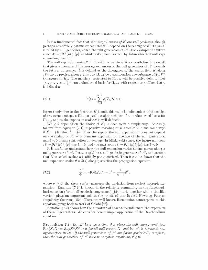
616 PIOTR T. CHRUSCIEL, GREGORY J. GALLOWAY, AND DANIEL POLLACK
It is a fundamental fact that the integral curves of K are null geodesics, thoughperhaps not affinely parameterized; this will depend on the scaling of K. Thus Nis ruled by null geodesics, called the null generators of N . For example the futurecone N = ∂I+(p) \ {p} in Minkowski space is ruled by future-directed null raysemanating from p.
The null expansion scalar θ of N with respect to K is a smooth function on Nthat gives a measure of the average expansion of the null generators of N towardsthe future. In essence, θ is defined as the divergence of the vector field K alongN . To be precise, given p ∈ N , let Πn−1 be a codimension-one subspace of TpN n
transverse to Kp. The metric g, restricted to Πn−1, will be positive definite. Let{e1, e2, . . . , en−1} be an orthonormal basis for Πn−1 with respect to g. Then θ at pis defined as
(7.1) θ(p) =n−1∑
i=1
g(∇eiK, ei) .
Interestingly, due to the fact that K is null, this value is independent of the choiceof transverse subspace Πn−1 as well as of the choice of an orthonormal basis forΠn−1, and so the expansion scalar θ is well defined.
While θ depends on the choice of K, it does so in a simple way. As easilyfollows from equation (7.1), a positive rescaling of K rescales θ in the same way:
if K = fK, then θ = fθ. Thus the sign of the null expansion θ does not dependon the scaling of K: θ > 0 means expansion on average of the null generators,and θ < 0 means contraction on average. In Minkowski space, the future null coneN = ∂I+(p) \ {p} has θ > 0, and the past cone N = ∂I−(p) \ {p} has θ < 0.
It is useful to understand how the null expansion varies as one moves along anull generator of N . Let s → η(s) be a null geodesic generator of N , and assumethat K is scaled so that η is affinely parameterized. Then it can be shown that thenull expansion scalar θ = θ(s) along η satisfies the propagation equation
(7.2)dθ
ds= −Ric(η′, η′)− σ2 − 1
n− 1θ2 ,
where σ ≥ 0, the shear scalar, measures the deviation from perfect isotropic ex-pansion. Equation (7.2) is known in the relativity community as the Raychaud-huri equation (for a null geodesic congruence) [154], and, together with a timelikeversion, plays an important role in the proofs of the classical Hawking–Penrosesingularity theorems [154]. There are well-known Riemannian counterparts to thisequation, going back to work of Calabi [63].
Equation (7.2) shows how the curvature of space-time influences the expansionof the null generators. We consider here a simple application of the Raychaudhuriequation.
Proposition 7.1. Let M be a space-time that obeys the null energy condition,Ric (X,X) = RαβX
αXβ ≥ 0 for all null vectors X, and let N be a smooth nullhypersurface in M . If the null generators of N are future geodesically complete,then the null generators of N have nonnegative expansion, θ ≥ 0.

MATHEMATICAL GENERAL RELATIVITY 617
Proof. Suppose θ < 0 at p ∈ N . Let η : [0,∞) → N , s → η(s), be the nullgeodesic generator of N passing through p = η(0). By rescaling K if necessary, wecan assume that η is affinely parameterized. Let θ = θ(s), s ∈ [0,∞), be the nullexpansion of N along η; hence θ(0) < 0. Raychaudhuri’s equation and the nullenergy condition imply that θ = θ(s) obeys the inequality
(7.3)dθ
ds≤ − 1
n− 1θ2 ,
and hence θ < 0 for all s > 0. Dividing through by θ2 then gives
(7.4)d
ds
(1
θ
)
≥ 1
n− 1,
which implies that 1/θ → 0, i.e., θ → −∞ in finite affine parameter time, contra-dicting the smoothness of θ. �
We wish to indicate the connection of Proposition 7.1 with the theory of blackholes. In fact, this proposition is the most rudimentary form of Hawking’s famousarea theorem [154]. Let M be a standard black hole space-time as defined, forexample, in [154]. It is not necessary to go into the technical details of the definition.It suffices to say that in M there exists a region B, the black hole region, from whichsignals (future-directed causal curves) cannot escape to infinity (recall the exampleof the Schwarzschild solution discussed in Section 3.1). The boundary of this regionis the event horizon E , which, in general, is a Lipschitz hypersurface ruled by futureinextendible null geodesics, called its null generators. If E is smooth and if itsgenerators are future-complete, then Proposition 7.1 implies that E has nonnegativenull expansion. This in turn implies that cross-sections of E are nondecreasing inarea as one moves towards the future, as asserted by the area theorem. In thecontext of black hole thermodynamics, the area theorem is referred to as the secondlaw of black mechanics, and provides a link between gravity and quantum physics.As it turns out, the area theorem remains valid without imposing any smoothnessassumptions; for a recent study of the area theorem, which focuses on these issuesof regularity, see [103].
7.2. Trapped and marginally trapped surfaces. We begin with some defini-tions. Let Σ = Σn−1, n ≥ 3, be a spacelike submanifold of codimension two in aspace-time (M n+1, g). Regardless of the dimension of space-time, we shall refer toΣ as a surface, which it actually is in the 3 + 1 case. We are primarily interestedin the case where Σ is compact (without boundary), and so we simply assume thisfrom the outset.
Each normal space of Σ, [TpΣ]⊥, p ∈ Σ, is timelike and two dimensional, and
hence, admits two future-directed null directions orthogonal to Σ. Thus, if thenormal bundle is trivial, Σ admits two smooth nonvanishing future-directed nullnormal vector fields l+ and l−, which are unique up to positive pointwise scaling;see Figure 7.1. By convention, we refer to l+ as outward pointing and l− as inwardpointing.14 In relativity it is standard to decompose the second fundamental formof Σ into two scalar-valued null second forms χ+ and χ−, associated to l+ and l−,respectively. For each p ∈ Σ, χ± : TpΣ× TpΣ → R is the bilinear form defined by
(7.5) χ±(X,Y ) = g(∇X l±, Y ) for all X,Y ∈ TpΣ .
14In many situations, there is a natural choice of inward and outward.

618 PIOTR T. CHRUSCIEL, GREGORY J. GALLOWAY, AND DANIEL POLLACK
l− l+
Figure 7.1. The null future normals l± to Σ.
A standard argument shows that χ± is symmetric. Hence, χ+ and χ− can be tracedwith respect to the induced metric γ on Σ to obtain the null mean curvatures (ornull expansion scalars)
(7.6) θ± = trγ χ± = γij(χ±)ij = divΣl± .
θ± depends on the scaling of l± in a simple way. As follows from equation (7.5),multiplying l± by a positive function f simply scales θ± by the same function.Thus, the sign of θ± does not depend on the scaling of l±. Physically, θ+ (resp.,θ−) measures the divergence of the outgoing (resp., ingoing) light rays emanatingfrom Σ.
It is useful to note the connection between the null expansion scalars θ± and theexpansion of the generators of a null hypersurface, as discussed in Section 7.1. LetN+ be the null hypersurface, defined and smooth near Σ, generated by the nullgeodesics passing through Σ with initial tangents l+. Then θ+ is the null expansionof N+ restricted to Σ. θ− may be described similarly.
Let M be a spacelike hypersurface in a space-time (M , g) with induced metrich and second fundamental form K, and suppose Σ is embedded as a two-sidedhypersurface in M . Then the null expansions θ± can be expressed in terms of theinitial data (M,h,K) as follows. Since Σ is two-sided in M , it admits a smoothunit normal field ν in M , unique up to sign. By convention, we refer to such achoice as outward pointing. Letting u denote the future-directed unit normal toM , l+ = u+ν (resp., l− = u−ν) is a future-directed outward (resp., future-directedinward) pointing null normal vector field along Σ. Let θ± be the null expansionwith respect to the null normal l±. Then
(7.7) θ± = trΣK ±H ,
where trΣK is the trace of the projection of K into Σ with respect to the inducedmetric on Σ, and H is the mean curvature of Σ in M .
For round spheres in Euclidean slices of Minkowski space, with the obvious choiceof inside and outside, one has θ− < 0 and θ+ > 0. In fact, this is the case in generalfor large radial spheres in asymptotically flat spacelike hypersurfaces. However, inregions of space-time where the gravitational field is strong, one may have bothθ− < 0 and θ+ < 0, in which case Σ is called a trapped surface. For example,the black hole region, 0 < r < 2m, in (n + 1)-dimensional Schwarzschild space-time (see Section 3.1) is foliated by spherically symmetric (n − 1)-spheres, all ofwhich are trapped surfaces. Under appropriate energy and causality conditions,the occurrence of a trapped surface signals the onset of gravitational collapse. Thisis the implication of the Penrose singularity theorem [238], the first of the famoussingularity theorems.

MATHEMATICAL GENERAL RELATIVITY 619
Theorem 7.2 (Penrose [238]). Let M be a globally hyperbolic space-time withnoncompact Cauchy surfaces satisfying the null energy condition. If M contains atrapped surface Σ, then M is future null geodesically incomplete.
Recall from Section 7.1 that the null energy condition is the curvature require-ment, Ric (X,X) = RαβX
αXβ ≥ 0 for all null vectors X. If a space-time M obeysthe Einstein equation (2.8), then one can express the null energy condition in termsof the energy momentum tensor: M obeys the null energy condition if and only ifT (X,X) = TijX
iXj ≥ 0 for all null vectors X.In studying an isolated gravitating system, such as the gravitational collapse of a
star, it is customary to model the situation by a space-time which is asymptoticallyflat. In this context the assumption of Theorem 7.2 that the space-time admits anoncompact Cauchy surface is natural. The conclusion in the theorem of futurenull geodesic incompleteness is an indication that space-time “comes to an end” ordevelops a singularity somewhere in the causal future. However, the theorem givesno information about the nature of the singularity.
The existence of vacuum asymptotically flat initial data sets, with one asymptoticregion and containing compact trapped surfaces, has been established by Beig andO Murchadha [34].
An intriguing question that arises in this context is whether a trapped surfacecan develop dynamically from initial data that did not contain any. This has beenaddressed by Christodoulou in [87], where a formidable analysis of the focusingeffect of sufficiently strong incoming gravitational waves is presented. Some furtherdevelopments can be found in [191].
To continue our discussion, consider again the general setting of a spacelikesurface Σn−1 in a space-time M n+1 with future-directed null normal fields l± andassociated null expansion scalars θ±. Focusing attention on just the outward nullnormal l+, we say that Σ is an outer trapped surface (resp., weakly outer trappedsurface) if θ+ < 0 (resp., θ+ ≤ 0). If θ+ vanishes, we say that Σ is a marginallyouter trapped surface, or MOTS for short. In what follows we will be primarilyconcerned with properties of MOTSs.
MOTSs arise naturally in a number of situations. As an outgrowth of theirwork on the positive energy theorem, Schoen and Yau [261] showed that suitableconditions on the energy density and momentum density of an asymptotically flatinitial data set ensure the presence of a MOTS; see also [286]. Next, as followsfrom our comments about the area theorem in Section 7.1, cross-sections of theevent horizon in black hole space-times have nonnegative expansion θ ≥ 0. (By across-section, we mean a smooth intersection of the event horizon with a spacelikehypersurface.) In the steady state limit this expansion goes to zero. Thus, it is abasic fact that cross-sections of the event horizon in stationary black hole space-times are MOTSs. For dynamical black hole space-times, MOTSs typically occurin the black hole region, i.e., the region inside the event horizon. While there areheuristic arguments for the existence of MOTSs in this situation, based on looking atthe boundary of the trapped region [154, 277] within a given spacelike slice, using anapproach put forth by Schoen [254], their existence has been rigorously establishedunder natural physical conditions, first by Andersson and Metzger [10] in dimensionthree, and then by Eichmair [131] up to dimension seven; see Section 7.5.
As noted earlier, MOTSs may be viewed as space-time analogues of minimalsurfaces in Riemannian geometry. In fact, as follows from equation (7.7), in the

620 PIOTR T. CHRUSCIEL, GREGORY J. GALLOWAY, AND DANIEL POLLACK
time-symmetric case (K = 0) a MOTS is simply a minimal surface in M . Ofimportance for certain applications is the fact, first discussed by Andersson, Marsand Simon [7, 8], that MOTSs admit a notion of stability analogous to that forminimal surfaces.
7.3. Stability of MOTSs. In Riemannian geometry, a minimal surface (surfacewith vanishing mean curvature) is stable provided, for a suitable class of variations,the second variation of area is nonnegative, δ2A ≥ 0. Stability of minimal surfacescan also be characterized in terms of the associated stability operator. This latterapproach extends to MOTSs, as we now describe.
Let Σ be a MOTS inM with outward unit normal ν. Consider a normal variationof Σ in M , i.e., a map F : (−ε, ε) × Σ → M , such that (i) F (0, ·) = idΣ and(ii) ∂F
∂t
∣∣t=0
= φν, φ ∈ C∞(Σ). Let θ(t) denote the null expansion of Σt := F (t,Σ)with respect to lt = u + νt, where u is the future-directed timelike unit normal toM and νt is the outer unit normal to Σt in M . A computation shows
(7.8)∂θ
∂t
∣∣∣∣t=0
= L(φ) ,
where L : C∞(Σ) → C∞(Σ) is the operator [8, 145]
(7.9) L(φ) = −�φ+ 2〈X,∇φ〉+(1
2S − (ρ+ J(ν))− 1
2|χ|2 + divX − |X|2
)
φ .
In the above, �, ∇, and div are the Laplacian, gradient and divergence operator,respectively, on Σ, S is the scalar curvature of Σ, ρ and J are the energy densityand momentum density, respectively, as defined in equations (5.3), (5.4), X is thevector field on Σ defined by taking the tangential part of ∇νu along Σ, and 〈 , 〉denotes the induced metric on Σ.
In the time-symmetric case, θ in (7.8) becomes the mean curvature H, the vectorfield X vanishes, and L reduces to the classical stability operator (linearizationof the mean curvature operator) of minimal surface theory. In analogy with theminimal surface case, we refer to L in (7.9) as the stability operator associatedwith variations in the null expansion θ. Although in general L is not self-adjoint,its principal eigenvalue (eigenvalue with smallest real part) λ1(L) is real. Moreover,there exists an associated eigenfunction φ which is positive on Σ. Continuing theanalogy with the minimal surface case, we say that a MOTS is stable providedλ1(L) ≥ 0. (In the minimal surface case this is equivalent to the second variationof area being nonnegative.) It follows from basic properties of L that a MOTS Σis stable if and only if there exists a normal variation of Σ, with φ > 0, such that∂θ∂t
∣∣t=0
≥ 0.Stable MOTSs arise naturally in physical situations, for example, as outermost
MOTSs. We say that Σ is an outermost MOTS in M provided there are no weaklyouter trapped (θ+ ≤ 0) surfaces outside of, and homologous to, Σ. We say that Σis a weakly outermost MOTS in M provided there are no outer trapped (θ+ < 0)surfaces outside of, and homologous to, Σ. Clearly, “outermost” implies “weaklyoutermost”. Moreover we have the following [7, 8]:
Proposition 7.3. Weakly outermost MOTSs are stable.
To see this, consider a variation {Σt} of a weakly outermost MOTS Σ withvariation vector field V = φν, where φ is a positive eigenfunction associated to theprincipal eigenvalue λ1 = λ1(L). If λ1 < 0, then equation (7.8) implies ∂θ
∂t
∣∣t=0
=

MATHEMATICAL GENERAL RELATIVITY 621
λ1φ < 0. Since θ(0) = 0, this implies that, for small t > 0, Σt is outer trapped,contrary to Σ being weakly outermost.
A standard fact in the theory of black holes is that, for black hole space-timesobeying the null energy condition, there can be no weakly outer trapped surfacescontained in the domain of outer communications (the region outside of all blackholes and white holes). It follows that compact cross-sections of the event horizonin stationary black hole space-times obeying the null energy condition are stableMOTSs. Moreover, results of Andersson and Metzger [9, 10] provide natural criteriafor the existence of outermost MOTSs in initial data sets containing trapped regions;see Section 7.5.
Stable MOTSs share a number of properties in common with stable minimalsurfaces. This sometimes depends on the following fact. Consider the symmetrizedoperator L0 : C∞(Σ) → C∞(Σ),
(7.10) L0(φ) = −�φ+
(1
2S − (ρ+ J(ν))− 1
2|χ|2
)
φ ,
formally obtained by setting X = 0 in (7.9). The key argument in [145] shows thefollowing (see also [8, 144]).
Proposition 7.4. λ1(L0) ≥ λ1(L).
In the next subsection we consider an application of stable MOTS to the topologyof black holes.
7.4. On the topology of black holes. A useful step in the proof of black holeuniqueness (see Section 3.7) is Hawking’s theorem on the topology of black holes[154], which asserts that compact cross-sections of the event horizon in (3 + 1)-dimensional, appropriately regular, asymptotically flat stationary black hole space-times obeying the dominant energy condition are topologically two-spheres. Asshown by Hawking [153], this conclusion also holds for outermost MOTSs in space-times that are not necessarily stationary. The proof in both cases is variational innature and relies on the classical Gauss–Bonnet theorem. Developments in physicsrelated to string theory have led to an increased interest in the study of gravity, andin particular black holes, in higher dimensions; see, e.g., [134] for a recent review.The remarkable example of Emparan and Reall [133] of a 4 + 1 asymptoticallyflat stationary vacuum black space-time with horizon topology S1 × S2, the so-called black ring, shows that horizon topology need not be spherical in higherdimensions. This example naturally led to the question of what are the allowablehorizon topologies in higher-dimensional black hole space-times. This questionwas addressed in the papers of [144, 145], resulting in a natural generalization ofHawking’s topology theorem to higher dimensions, which we now discuss.
Consider a space-time (M n+1, g), n ≥ 3, satisfying the Einstein equations (notnecessarily vacuum), and for simplicity assume that the cosmological constant van-ishes, Λ = 0. Let M be a spacelike hypersurface in M , which gives rise to the initialdata set (M,h,K), as in Section 7.3. Recall from equation (5.15) that the dominantenergy condition holds with respect to this initial data set provided ρ ≥ |J | alongM , where ρ and J are the energy density and momentum density, respectively, asdefined in Section 5.1 (but with Λ set to zero).
The following result, obtained in [145], gives a natural extension of Hawking’sblack hole topology theorem to higher dimensions. Recall that a Riemannian man-ifold Σ is of positive Yamabe type if it admits a metric of positive scalar curvature.

622 PIOTR T. CHRUSCIEL, GREGORY J. GALLOWAY, AND DANIEL POLLACK
Theorem 7.5. Let Σn−1 be a stable MOTS in an initial data set (Mn, h,K),n ≥ 3.
(1) If ρ > |J | along Σ, then Σ is of positive Yamabe type.(2) If ρ ≥ |J | along Σ, then Σ is of positive Yamabe type unless Σ is Ricci flat
(flat if n = 2, 3), χ = 0 and ρ+ J(ν) = 0 along Σ.
In the time-symmetric case, Theorem 7.5 reduces to the classical result of Schoenand Yau [258], critical to their study of manifolds of positive scalar curvature, thata compact stable minimal hypersurface in a Riemannian manifold of positive scalarcurvature is of positive Yamabe type.
The key to the proof of Theorem 7.5 is Proposition 7.4, which, since Σ is assumedstable, implies that λ1(L0) ≥ 0, where L0 is the operator given in (7.10). Now,in effect, the proof has been reduced to the Riemannian case. Consider Σ in the
conformally related metric, γ = φ2
n−2 γ, where γ is the induced metric on Σ and φis a positive eigenfunction corresponding to λ1(L0). The scalar curvatures S andS of the metrics γ and γ, respectively, are related by (compare (5.11))
S = φ− nn−2
(
−2�φ+ Sφ+n− 1
n− 2
|∇φ|2φ
)
= φ− 2n−2
(
2λ1(L0) + 2(ρ+ J(ν)) + |χ|2 + n− 1
n− 2
|∇φ|2φ2
)
,
where for the second equation we have used (7.10). Since ρ + J(ν) ≥ ρ − |J | ≥ 0,
we have that S ≥ 0. By further standard metric deformations, the scalar curvatureof Σ can be made strictly positive, unless various quantities vanish identically.
According to Theorem 7.5, apart from certain exceptional circumstances, a stablemarginally outer trapped surface Σ in a space-time M obeying the dominant energycondition is of positive Yamabe type. Assume for the following discussion that Σis orientable. Then, in the standard case: dimM = 3 + 1 (and hence dimΣ = 2),Gauss–Bonnet tells us that if Σ is positive Yamabe, then Σ is topologically a two-sphere, and we recover Hawking’s theorem. In higher dimensions, much is nowknown about topological obstructions to the existence of metrics of positive scalarcurvature. While the first major result along these lines is the famous theoremof Lichnerowicz [198] concerning the vanishing of the A genus, a key advance inour understanding was made in the late 1970s and early 1980s by Schoen andYau [256, 258] and Gromov and Lawson [147, 148]. Let us focus on the case:dim M = 4 + 1, and hence dim Σ = 3. Then by results of Schoen–Yau andGromov-Lawson, in light of the resolution of the Poincare conjecture, Σ must bediffeomorphic to a finite connected sum of spherical spaces (spaces which are coveredby the three-sphere) and S2 × S1’s. Indeed, by the prime decomposition theorem,Σ can be expressed as a connected sum of spherical spaces, S2 × S1’s, and K(π, 1)manifolds (manifolds whose universal covers are contractible). But as Σ admitsa metric of positive scalar curvature, it cannot have any K(π, 1)’s in its primedecomposition. Hence, the basic horizon topologies in dim M = 4 + 1 are S3
and S2 × S1 (in the sense that Σ is “built up” from such spaces), both of whichare realized by nontrivial black hole space-times. It remains an interesting openquestion which topologies of positive Yamabe type can be realized as outermostMOTSs; see [264] for examples involving products of spheres.
A drawback of Theorem 7.5 is that it allows certain possibilities that one wouldlike to rule out. For example, the theorem does not rule out the possibility of a

MATHEMATICAL GENERAL RELATIVITY 623
vacuum black hole space-time with toroidal horizon topology (this borderline casealso arises in the proof of Hawking’s theorem). In fact, one can construct examplesof stable toroidal MOTSs in space-times obeying the dominant energy condition.Such MOTSs cannot, however, be outermost, as the following theorem asserts.
Theorem 7.6 ([144]). Let Σ be an outermost MOTS in the spacelike hypersur-face M and assume the dominant energy condition (3.15) holds in a space-timeneighborhood of Σ.15 Then Σ is of positive Yamabe type.
As an immediate corollary, we have that compact cross-sections of event horizonsin regular stationary black hole space-times obeying the dominant energy conditionare of positive Yamabe type. In particular, there can be no toroidal horizons.
Theorem 7.6 is an immediate consequence of the following rigidity result.
Theorem 7.7 ([144]). Let Σ be a weakly outermost MOTS in the spacelike hy-persurface M and assume the dominant energy condition holds in a space-timeneighborhood of Σ. If Σ is not of positive Yamabe type, then there exists an outerneighborhood U ≈ [0, ε)× Σ of Σ in M such that each slice Σt = {t} × Σ, t ∈ [0, ε)is a MOTS.
Theorem 7.7 is proved in two stages. The first stage, and the main effort, is toestablish Theorem 7.7 subject to the additional assumption that M has nonpositivemean curvature, τ ≤ 0. This is a purely initial data result, and the proof is carriedout in two steps. The first step involves an inverse function theorem argument toshow that an outer neighborhood of Σ can be foliated by surfaces Σt of constantnull expansion, θ(t) = ct. This uses the stability of Σ in a critical way. In thesecond step it is shown that all of these constants are zero, ct = 0. It is here wherethe sign of the mean curvature of M needs to be controlled. Once having provedTheorem 7.7, subject to the condition, τ ≤ 0, the next stage, which is actually easy,is a deformation argument (specifically, a deformation of M near Σ) that reducesthe problem to the case τ ≤ 0.
We remark that Riemannian versions of Theorem 7.7 had previously been con-sidered in [61, 62].
7.5. Existence of MOTSs. As mentioned earlier, compact cross-sections of theevent horizon in regular stationary black hole space-times are necessarily MOTSs.In dynamical black hole space-times, it is typical for trapped or outer trappedsurfaces to form in the black hole region. But the occurrence of an outer trappedsurface in a spacelike hypersurface that obeys a mild asymptotic flatness conditionleads to the existence of a MOTS. This follows from the existence result alluded tonear the end of Section 7.2, and which we now discuss [10, 131, 254].
Let Ω be a relatively compact domain in a spacelike hypersurface M with smoothboundary ∂Ω. We assume that ∂Ω decomposes as a disjoint union of components,∂Ω = Σinn ∪ Σout, where we think of Σinn as the inner boundary and Σout as theouter boundary of Ω in M . We choose the normal along Σinn that points into Ω,and the normal along Σout that points out of Ω, so that both normals point towardsthe region exterior to Σout. Thus, Σinn is outer trapped if θ < 0 with respect to thefuture-directed null normal field along Σinn that projects into Ω. We say that Σout
15Note that since we are assuming Λ = 0 here, the dominant energy condition is equivalentto the condition, GρνXρY ν ≥ 0 for all future-directed causal vectors X,Y , where Gμν is the
Einstein tensor.

624 PIOTR T. CHRUSCIEL, GREGORY J. GALLOWAY, AND DANIEL POLLACK
is outer untrapped if θ > 0 with respect to the future-directed null normal alongΣout that projects out of Ω. Heuristically, if Σout is lying in a region where M isflattening out, then we expect Σout to be outer untrapped.
With this notation and terminology we have the following existence result forMOTS.
Theorem 7.8 ([10, 131]). Let Mn be a spacelike hypersurface in a space-time(M n+1, g), with n ≤ 7. Let Ω be a relatively compact domain in M , with smoothboundary ∂Ω = Σinn ∪Σout, such that the inner boundary Σinn is outer trapped andthe outer boundary Σout is outer untrapped, as described above. Then there existsa smooth compact MOTS in Ω homologous to Σinn.
Moreover, it has been shown that the MOTS constructed in Theorem 7.8 isstable ([10, 5]).
In the time-symmetric case, Theorem 7.8 reduces to a well-known existence re-sult for stable minimal surfaces. In this case the barrier conditions in Theorem7.8 simply say that Ω is a mean convex domain. One can then minimize area inthe homology class of a surface in Ω parallel to Σinn and apply standard compact-ness and regularity results of geometric measure theory [137] to obtain a smooth(provided dimM ≤ 7) stable minimal surface in Ω homologous to Σinn. However,since MOTSs do not arise as stationary points of some elliptic functional, such aprocedure does not work for general initial data. A completely different approachmust be taken.
In fact, the proof of Theorem 7.8 is based on Jang’s equation [180], which isclosely related to the MOTS condition θ+ = 0. Given an initial data set (M, g,K),
consider the Riemannian product manifold, M = R×M , g = dt2 + g, and extendK to M by taking it to be constant along the t-lines. Given a function f on M ,consider its graph, Nf = graph f = {(t, x) ∈ M : t = f(x), x ∈ M}, equipped withthe induced metric. Then Jang’s equation is the equation
(7.11) (H + P )(f) = H(f) + P (f) = 0 ,
where H(f) = the mean curvature of Nf and P = trNfK (compare with equation
(7.7)).Schoen and Yau [260] established existence and regularity for Jang’s equation
with respect to asymptotically flat initial sets as part of their approach to provingthe positive mass theorem for general, nonmaximal, initial data sets. In the processthey discovered an obstruction to global existence: solutions to Jang’s equation tendto blow up in the presence of MOTS in the initial data (M, g,K). This problematicblow-up behavior that Schoen and Yau had to contend with has now been turned onits head to become a feature of Jang’s equation: in order to establish the existenceof MOTS, one induces a blowup of the Jang equation. This is the approach takenin [10, 131] in a somewhat different situation.
In order to obtain solutions to Jang’s equation, one considers the regularizedequation
(7.12) (H + P )(ft) = tft .
In [131], Eichmair uses a Perron method to obtain solutions ft to (7.12) for tsufficiently small, with values that tend to infinity in a small collared neighborhoodof Σout, and that tend to minus infinity in a small collared neighborhood of Σinn,as t → 0. The construction of Perron subsolutions and supersolutions makes use of

MATHEMATICAL GENERAL RELATIVITY 625
the barrier conditions. Using the almost minimizing property [131] of the graphsNt := graph ft, one is able to pass to a smooth subsequential limit manifold N ,bounded away from ∂Ω, each component of which is either a cylinder or a graphthat asymptotes to a cylinder. The projection into M of such a cylinder producesthe desired MOTS.
Under the barrier conditions of Theorem 7.8, Andersson and Metzger [10] wereable to make use of this basic existence result to establish, for three-dimensionalinitial data sets, the existence of an outermost MOTS, thereby providing a rigorousproof of a long held “folk belief” in the theory of black holes that the boundary ofthe so-called outer trapped region in a time slice of space-time is a smooth MOTS.The key to proving the existence of an outermost MOTS is a compactness resultfor stable MOTS which follows from the extrinsic curvature estimates obtainedby Andersson and Metzger in [9], together with an area bound obtained in [10].This area bound follows from an outer injectivity radius estimate for a certainclass of MOTS, established by an interesting surgery procedure. The powerfulmethods developed by Eichmair in [130, 131] can be used to extend this result ton-dimensional initial data sets, 3 ≤ n ≤ 7.
Consider, now, a foliation {Mt}, a < t < b, of a region of a space-time (M n+1, g)by spacelike hypersurfaces Mt. If each slice Mt admits an outermost MOTS Σt,then the family of MOTSs {Σt} may form a hypersurface in space-time. A smoothspacelike hypersurface H in a space-time (M n+1, g) foliated by MOTS is called amarginally outer trapped tube (MOTT). In [7, 8], Andersson, Mars and Simon haveobtained a rigorous existence result for MOTTs. Consider a spacelike foliation{Mt}, a < t < b, and suppose Σt0 is a MOTS in Mt0 . They prove that if Σt0 isstrictly stable, i.e., if the principal eigenvalue of the associated stability operator(7.9) is strictly positive, then there exists a MOTT H such that for t close to t0,Σt := H ∩Mt is a MOTS. For further related results see [6].
Many challenging questions concerning the global existence and behavior ofMOTTs remain open. Building on the analysis of Dafermos [117], Williams [283]gave sufficient conditions on spherically symmetric black hole space-times satisfyingthe dominant energy condition, insuring that a spherically symmetric MOTT ex-ists, is achronal, and is asymptotic to the event horizon. Understanding the genericasymptotic behavior of MOTTs in the nonspherically symmetric case remains aninteresting open problem.
A MOTT satisfying certain supplementary conditions gives rise to the notionof a dynamical horizon, which provides an alternative, quasi-local description of ablack hole. For an extensive review of dynamical horizons and related concepts,including physical applications, see [17].
Appendix A. Open problems
We compile here a list of interesting open problems discussed in the paper. Theyall appear to be difficult, of varying degrees of difficulty, with some most likelyintractable in the foreseeable future.
(1) Remove the hypotheses of analyticity, nondegeneracy, and connectednessin the black hole uniqueness Theorem 3.2, p. 585.
(2) Construct a five-dimensional, stationary, I+-regular vacuum black hole withtwo-dimensional group of isometries, or show that there are no such blackholes. More generally, classify such black holes. Compare p. 586.

626 PIOTR T. CHRUSCIEL, GREGORY J. GALLOWAY, AND DANIEL POLLACK
(3) Prove that the positive energy theorem holds in all dimensions without thespin assumption. Compare p. 596.
(4) Find the optimal differentiability conditions for Theorem 4.1. More gen-erally, construct a coherent local well-posedness theory for the evolutionand constraint equations for metrics with low differentiability. CompareRemark 4.2, p. 588.
(5) Describe in a constructive way the set of solutions of the vacuum constraintequations on compact, asymptotically flat, and asymptotically hyperbolicmanifolds, with arbitrary smooth initial data. Compare p. 594.
(6) Formulate, and prove, a precise version of Conjecture 6.9, p. 614. Moregenerally, formulate and prove a precise version of the BKL conjecture, orfind an open set of metrics developing a singularity which do not exhibit aBKL-type behavior.
(7) Show that generic Bianchi IX orbits have a dense ω-limit set on the Kasnercircle. Compare p. 612.
(8) Show that uniqueness and existence of maximal globally hyperbolic devel-opments (Theorem 6.1, p. 602) holds in an optimal weak differentiabilityclass. This requires revisiting the whole causality theory for metrics of lowdifferentiability.
(9) Remove the condition of closed generators in Theorem 6.2, p. 602. Moregenerally, show that existence of Cauchy horizons, not necessarily compactor analytic, implies existence of local isometries, or construct a counterex-ample.
(10) Generalize Ringstrom’s Theorem 6.3, p. 603, to Gowdy models on S2×S1,on S3, and on lens spaces L(p, q).
(11) Show that some twisting U(1)×U(1)-symmetric vacuum models on T3 have
mixmaster behavior. More generally, find an open set of such models withmixmaster behavior. Even better, analyze exhaustively the asymptoticbehavior of those models; see Section 6.1.2, p. 604.
(12) Show that degenerate asymptotically flat spherically symmetric Einstein–Maxwell scalar field solutions are nongeneric. Compare Section 6.1.3, p. 605.Analyze what happens in solutions in which trapped surfaces do not form.More generally, prove weak and strong cosmic censorship within this classof space-times.
(13) Find an open set of U(1)-symmetric metrics where the dynamics can beanalyzed in the contracting direction. More generally, analyze exhaustivelythe dynamics of those models; see Section 6.3.1, p. 606.
(14) Show that polyhomogeneous initial data in Theorem 6.6, p. 609, lead tosolutions with polyhomogeneous behavior at null infinity.
(15) Show that the Kerr solution is stable against small vacuum perturbations.Compare Section 6.5, p. 610.
(16) Determine what topologies of positive Yamabe type can be realized as out-ermost MOTSs in space-times satisfying the dominant energy condition.Compare p. 622.
(17) Prove initial data equivalents of Theorems 7.6 and 7.7, p. 623.(18) Describe the generic behavior near the event horizon of marginally trapped
tubes in black hole space-times; see p. 625.

MATHEMATICAL GENERAL RELATIVITY 627
Acknowledgments
We are grateful to the Banff International Research Station and to the Mittag-Leffler Institute for hospitality at various stages of work on this project. Thefirst and third authors acknowledge the friendly hospitality of the University ofMiami during part of the work on this paper. We are indebted to Jim Isenbergand Catherine Williams for many useful comments on a previous version of themanuscript. Further thanks are due to Catherine Williams for providing somefigures and for helping with others and to Woei-Chet Lim for providing Figure 6.2.
About the authors
Piotr T. Chrusciel is professor of gravitational physics at the University of Vi-enna. His research focuses on global problems arising in Einstein’s theory of gravi-tation. Greg Galloway is professor of mathematics at the University of Miami. Hisprimary research interests are in space-time geometry and mathematical relativity.Daniel Pollack is professor of mathematics at the University of Washington. Hisresearch areas include geometric analysis, partial differential equations, and generalrelativity.
References
1. S. Alexakis, A.D. Ionescu, and S. Klainerman, Hawking’s local rigidity theorem withoutanalyticity, (2009), arXiv:0902.1173.
2. P. Allen, A. Clausen, and J. Isenberg, Near-constant mean curvature solutions of the Einsteinconstraint equations with non-negative Yamabe metrics, Class. Quantum Grav. 25 (2008),075009, 15 pp., arxiv:0710.0725v1[gr-qc]. MR2404418 (2009a:83009)
3. L. Andersson, The global existence problem in general relativity, The Einstein Equationsand the Large Scale Behavior of Gravitational Fields (P.T. Chrusciel and H. Friedrich, eds.),Birkhauser, Basel, 2004, arXiv:gr-qc/9911032v4, pp. 71–120. MR2098914 (2005k:58054)
4. L. Andersson and P. Blue, Hidden symmetries and decay for the wave equation on the Kerrspacetime, (2009), arXiv:0908.2265 [math.AP].
5. L. Andersson, M. Eichmair, and J. Metzger, Jang’s equation and its applications tomarginally trapped surfaces (2010), arXiv:1006.4601.
6. L. Andersson, M. Mars, J. Metzger, and W. Simon, The time evolution of marginally trappedsurfaces, Class. Quant. Grav. 26 (2009), 085018.
7. L. Andersson, M. Mars, and W. Simon, Local existence of dynamical and trapping horizons,Phys. Rev. Lett. 95 (2005), 111102.
8. , Stability of marginally outer trapped surfaces and existence of marginally outertrapped tubes, Adv. Theor. Math. Phys. 12 (2008), 853–888. MR2420905 (2010a:83005)
9. L. Andersson and J. Metzger, Curvature estimates for stable marginally trapped surfaces,(2005), arXiv:gr-qc/0512106.
10. , The area of horizons and the trapped region, arXiv:0708.4252 [gr-qc]. Comm. Math.Phys. 290 (2009), 941–972. MR2525646 (2010f:53118)
11. L. Andersson and V. Moncrief, Einstein spaces as attractors for the Einstein flow, in prepa-ration.
12. , Elliptic-hyperbolic systems and the Einstein equations, Ann. Henri Poincare 4(2003), 1–34, arXiv:gr-qc/0110111. MR1967177 (2004c:58060)
13. , Future complete vacuum space-times, The Einstein Equations and the Large ScaleBehavior of Gravitational Fields (P.T. Chrusciel and H. Friedrich, eds.), Birkhauser, Basel,2004, pp. 299–330, arXiv:gr–qc/0303045. MR2098919 (2006c:83004)
14. L. Andersson and A.D. Rendall, Quiescent cosmological singularities, Commun. Math. Phys.218 (2001), 479–511, arXiv:gr-qc/0001047. MR2002h:83072
15. R. Arnowitt, S. Deser, and C.W. Misner, The dynamics of general relativity, Gravitation: Anintroduction to current research, Wiley, New York, 1962, pp. 227–265. MR0143629 (26:1182)

628 PIOTR T. CHRUSCIEL, GREGORY J. GALLOWAY, AND DANIEL POLLACK
16. A. Ashtekar and G.J. Galloway, Some uniqueness results for dynamical horizons, Adv. Theor.Math. Phys. 9 (2005), 1–30. MR2193368 (2006k:83101)
17. A. Ashtekar and B. Krishnan, Isolated and dynamical horizons and their applications, LivingRev. Rel. 7 (2004), gr-qc/0407042.
18. J.D. Barrow and F.J. Tipler, Analysis of the generic singularity studies by Belinskiı, Kha-latnikov, and Lifschitz, Phys. Rep. 56 (1979), 371–402. MR555355 (83c:83005)
19. R. Bartnik, The existence of maximal hypersurfaces in asymptotically flat space-times, Com-
mun. Math. Phys. 94 (1984), 155–175. MR761792 (86b:53063)20. , The mass of an asymptotically flat manifold, Commun. Pure Appl. Math. 39 (1986),
661–693. MR849427 (88b:58144)21. , Regularity of variational maximal surfaces, Acta Math. 161 (1988), 145–181.
MR971795 (90b:58255)22. , Remarks on cosmological spacetimes and constant mean curvature surfaces, Com-
mun. Math. Phys. 117 (1988), 615–624. MR953823 (89g:53094)23. , Some open problems in mathematical relativity, Conference on Mathematical Rela-
tivity (Canberra, 1988), Proc. Centre Math. Anal. Austral. Nat. Univ., vol. 19, Austral. Nat.Univ., Canberra, 1989, pp. 244–268. MR1020805 (90g:83001)
24. , Phase space for the Einstein equations, Commun. Anal. Geom. 13 (2005), 845–885,arXiv:gr-qc/0402070. MR2216143 (2007d:83012)
25. R. Bartnik, P.T. Chrusciel, and N. O Murchadha, On maximal surfaces in asymptoticallyflat space-times., Commun. Math. Phys. 130 (1990), 95–109. MR1055687 (91b:53078)
26. R. Bartnik and J. Isenberg, The constraint equations, The Einstein equations and thelarge scale behavior of gravitational fields, Birkhauser, Basel, 2004, pp. 1–38. MR2098912(2005j:83007)
27. J.K. Beem, P.E. Ehrlich, and K.L. Easley, Global Lorentzian geometry, Second ed., MarcelDekker Inc., New York, 1996. MR1384756 (97f:53100)
28. F. Beguin, Aperiodic oscillatory asymptotic behavior for some Bianchi spacetimes, (2010),arXiv:1004.2984 [gr-qc].
29. R. Beig, TT-tensors and conformally flat structures on 3-manifolds, Mathematics of Grav-itation, Part I (Warsaw, 1996), Banach Center Publ., vol. 41, Polish Acad. Sci., Warsaw,1997, pp. 109–118. MR1466511 (98k:53040)
30. R. Beig and P.T. Chrusciel, Killing Initial Data, Class. Quantum. Grav. 14 (1997), A83–A92, A special issue in honour of Andrzej Trautman on the occasion of his 64th Birthday,J.Tafel, editor. MR1691888 (2000c:83011)
31. , Killing vectors in asymptotically flat space-times: I. Asymptotically translationalKilling vectors and the rigid positive energy theorem, Jour. Math. Phys. 37 (1996), 1939–1961, arXiv:gr-qc/9510015. MR1380882 (97d:83033)
32. , The asymptotics of stationary electro-vacuum metrics in odd space-time dimensions,Class. Quantum Grav. 24 (2007), 867–874. MR2297271
33. R. Beig, P.T. Chrusciel, and R. Schoen, KIDs are non-generic, Ann. Henri Poincare 6 (2005),155–194, arXiv:gr-qc/0403042. MR2121280 (2005m:83013)
34. R. Beig and N. O Murchadha, Vacuum spacetimes with future trapped surfaces, Class. Quan-tum Grav. 13 (1996), 739–751. MR1383704 (97e:83005)
35. V.A. Belinski, I.M. Khalatnikov, and E.M. Lifshtitz, Oscillatory approach to a singular pointin the relativistic cosmology, Adv. Phys. 19 (1970), 525–573.
36. B. Berger, P.T. Chrusciel, J. Isenberg, and V. Moncrief, Global foliations of vacuum space-times with T 2 isometry, Ann. Phys. (NY) 260 (1997), 117–148. MR1474313 (98j:83005)
37. B. Berger, J. Isenberg, and M. Weaver, Oscillatory approach to the singularity in vac-
uum space-times with T 2 isometry, Phys. Rev. D64 (2001), 084006, arXiv:gr-qc/0104048,erratum-ibid. D67, 129901 (2003).
38. B.K. Berger, Hunting local mixmaster dynamics in spatially inhomogeneous cosmologies,Class. Quantum Grav. 21 (2004), S81–S95, A space-time safari: Essays in honour of VincentMoncrief. MR2053000 (2005f:83066)
39. B.K. Berger, D. Garfinkle, J. Isenberg, V. Moncrief, and M. Weaver, The singularity ingeneric gravitational collapse is spacelike, local, and oscillatory, Mod. Phys. Lett. A13(1998), 1565–1574, arXiv:gr-qc/9805063. MR1633408 (99j:83052)
40. B.K. Berger and V. Moncrief, Exact U(1) symmetric cosmologies with local Mixmaster dy-namics, Phys. Rev. D62 (2000), 023509, arXiv:gr-qc/0001083. MR1790740 (2001f:83027)

MATHEMATICAL GENERAL RELATIVITY 629
41. , Signature for local mixmaster dynamics in U(1) symmetric cosmologies, Phys. Rev.D 62 (2000), 123501, 9, arXiv:gr-qc/0006071. MR1813870 (2001k:83027)
42. A.N. Bernal and M. Sanchez, Smoothness of time functions and the metric splitting ofglobally hyperbolic space-times, Commun. Math. Phys. 257 (2005), 43–50. MR2163568(2006g:53105)
43. A.L. Besse, Einstein manifolds, Ergebnisse der Mathematik und ihrer Grenzgebiete. 3. Folge,vol. 10, Springer Verlag, Berlin, New York, Heidelberg, 1987. MR867684 (88f:53087)
44. L. Bieri and N. Zipser, Extensions of the stability theorem of the Minkowski space in generalrelativity. AMS/IP Studies in Advanced Mathematics, vol. 45, Amer. Math. Soc., Providence,RI, 2009. MR2531716
45. G. D. Birkhoff, Relativity and modern physics, Harvard University Press, 1923.46. P. Blue, Decay of the Maxwell field on the Schwarzschild manifold, arXiv:0710.4102
[math.AP]. J. Hyperbolic Differ. Equ. 5 (2008), 807–856. MR2475482 (2010d:35371)47. P. Blue and J. Sterbenz, Uniform decay of local energy and the semi-linear wave equation
on Schwarzchild space, arXiv:math.AP/0510315. Comm. Math. Phys. 268 (2006), 481–504.MR2259204 (2007i:58037)
48. H.L. Bray, Proof of the Riemannian Penrose inequality using the positive mass theorem,Jour. Diff. Geom. 59 (2001), 177–267. MR1908823 (2004j:53046)
49. , Black holes and the Penrose inequality in general relativity, Proceedings of theInternational Congress of Mathematicians, Vol. II (Beijing, 2002), Higher Ed. Press, 2002,pp. 257–271. MR1957038 (2004b:83056)
50. , Black holes, geometric flows, and the Penrose inequality in general relativity, No-tices Amer. Math. Soc. 49 (2002), 1372–1381. MR1936643 (2003j:83052)
51. H.L. Bray and P.T. Chrusciel, The Penrose inequality, The Einstein Equations and the LargeScale Behavior of Gravitational Fields (P.T. Chrusciel and H. Friedrich, eds.), Birkhauser,Basel, 2004, pp. 39–70, arXiv:gr–qc/0312047. MR2098913 (2005m:83014)
52. H.L. Bray and M.A. Khuri, A Jang Equation Approach to the Penrose Inequality, (2009),arXiv:0910.4785 [math.DG].
53. , PDE’s which imply the Penrose conjecture, (2009), arXiv:0905.2622 [math.DG].54. H.L. Bray and D.A. Lee, On the Riemannian Penrose inequality in dimensions less than
eight, Duke Math. Jour. 148 (2009), 81–106, arXiv:0705.1128. MR251510155. H.L. Bray and P. Miao, On the capacity of surfaces in manifolds with nonnegative scalar
curvature, Invent. Math. 172 (2008), 459–475. MR239307656. H.L. Bray and R. Schoen, Recent proofs of the Riemannian Penrose conjecture, Current
Developments in Mathematics, 1999 (Cambridge, MA), Int. Press, Somerville, MA, 1999,pp. 1–36. MR1990246 (2004j:53047)
57. Hubert Bray, Sean Hayward, Marc Mars, and Walter Simon, Generalized inverse mean cur-vature flows in spacetime, Commun. Math. Phys. 272 (2007), 119–138, arXiv:gr-qc/0603014.MR2291804 (2008c:53065)
58. P. Breitenlohner, D. Maison, and G. Gibbons, 4-dimensional black holes from Kaluza-Kleintheories, Commun. Math. Phys. 120 (1988), 295–333. MR973537 (89j:83018)
59. R. Brout, S. Massar, R. Parentani, and P. Spindel, A primer for black hole quantum physics,Phys. Rept. 260 (1995), 329–454. MR1353182 (97g:83064)
60. R. Budic, J. Isenberg, L. Lindblom, and P. Yasskin, On the determination of the Cauchysurfaces from intrinsic properties, Commun. Math. Phys. 61 (1978), 87–95. MR0489695(58:9089)
61. M. Cai, Volume minimizing hypersurfaces in manifolds of nonnegative scalar curvature,Minimal Surfaces, Geometric Analysis and Symplectic Geometry (Baltimore, MD, 1999),Adv. Stud. Pure Math., vol. 34, Math. Soc. Japan, Tokyo, 2002, pp. 1–7. MR1925731(2003f:53104)
62. M. Cai and G.J. Galloway, Rigidity of area minimizing tori in 3-manifolds of nonnegativescalar curvature, Commun. Anal. Geom. 8 (2000), 565–573. MR1775139 (2001j:53051)
63. E. Calabi, On Ricci curvature and geodesics, Duke Math. J. 34 (1967), 667–676. MR0216429
(35:7262)64. A. Carrasco and M. Mars, A counter-example to a recent version of the Penrose conjecture,
(2009), arXiv:0911.0883 [gr-qc].65. B. Carter, Global structure of the Kerr family of gravitational fields, Phys. Rev. 174 (1968),
1559–1571.

630 PIOTR T. CHRUSCIEL, GREGORY J. GALLOWAY, AND DANIEL POLLACK
66. , Black hole equilibrium states, Black Holes (C. de Witt and B. de Witt, eds.), Gordon& Breach, New York, London, Paris, 1973, Proceedings of the Les Houches Summer School.MR0465047 (57:4960)
67. M. Chae and P.T. Chrusciel, On the dynamics of Gowdy space times, Commun. Pure Appl.Math. 57 (2004), 1015–1074, arXiv:gr-qc/0305029. MR2053758 (2005i:83085)
68. Y. Choquet-Bruhat, Positive-energy theorems, Relativity, groups and topology, II (LesHouches, 1983) (B.S. deWitt and R. Stora, eds.), North-Holland, Amsterdam, 1984, pp. 739–
785. MR830248 (87g:83054)69. , Einstein constraints on compact n-dimensional manifolds, Class. Quantum Grav.
21 (2004), S127–S151, arXiv:gr-qc/0311029. MR2053003 (2005g:83011)70. , Future complete U(1) symmetric Einsteinian space-times, the unpolarized case, The
Einstein Equations and the Large Scale Behavior of Gravitational Fields (P.T. Chrusciel andH. Friedrich, eds.), Birkhauser, Basel, 2004, pp. 251–298. MR2098918 (2006b:83015)
71. , General relativity and the Einstein equations, Oxford University Press, Oxford, UK,2009. MR2473363
72. Y. Choquet-Bruhat and D. Christodoulou, Elliptic systems in Hs,δ spaces on manifoldswhich are Euclidean at infinity, Acta Math. 146 (1981), 129–150. MR594629 (82c:58060)
73. Y. Choquet-Bruhat, P.T. Chrusciel, and J. Loizelet, Global solutions of the Einstein–Maxwell equations in higher dimension, Class. Quantum Grav. (2006), 7383–7394, arXiv:gr-qc/0608108. MR2279722 (2008i:83022)
74. Y. Choquet-Bruhat, P.T. Chrusciel, and J.M. Martın-Garcıa, The light-cone theorem, Class.Quantum Grav. 26 (2009), 135011 (22 pp.), arXiv:0905.2133 [gr-qc]. MR2515694
75. Y. Choquet-Bruhat and R. Geroch, Global aspects of the Cauchy problem in general relativ-ity, Commun. Math. Phys. 14 (1969), 329–335. MR0250640 (40:3872)
76. Y. Choquet-Bruhat, J. Isenberg, and V. Moncrief, Solutions of constraints for Einsteinequations, C. R. Acad. Sci. Paris Ser. I Math. 315 (1992), 349–355. MR1179734 (93h:58151)
77. Y. Choquet-Bruhat, J. Isenberg, and D. Pollack, The Einstein-scalar field constraints onasymptotically Euclidean manifolds, Chinese Ann. Math. Ser. B 27 (2006), 31–52, arXiv:gr-qc/0506101. MR2209950 (2007h:58049)
78. , Applications of theorems of Jean Leray to the Einstein-scalar field equations, Jour.
Fixed Point Theory Appl. 1 (2007), 31–46, arXiv:gr-qc/0611009. MR228234279. , The constraint equations for the Einstein-scalar field system on compact manifolds,
Class. Quantum Grav. 24 (2007), 809–828, arXiv:gr-qc/0610045. MR229726880. Y. Choquet-Bruhat and V. Moncrief, Future global in time Einsteinian space-times with
U(1) isometry group., Ann. Henri Poincare 2 (2001), 1007–1064. MR1877233 (2003g:53123)81. Y. Choquet-Bruhat and J. York, The Cauchy problem, General Relativity (A. Held, ed.),
Plenum Press, New York, 1980, pp. 99–172. MR583716 (82k:58028)82. D. Christodoulou, Global solutions of nonlinear hyperbolic equations for small initial data,
Commun. Pure Appl. Math. 39 (1986), 267–282. MR820070 (87c:35111)83. , The problem of a self-gravitating scalar field, Commun. Math. Phys. 105 (1986),
337–361. MR848643 (87i:83009)84. , Examples of naked singularity formation in the gravitational collapse of a scalar
field, Ann. of Math. (2) 140 (1994), 607–653. MR1307898 (95j:83100)85. , The instability of naked singularities in the gravitational collapse of a scalar field,
Ann. of Math. (2) 149 (1999), 183–217. MR1680551 (2000a:83086)86. , On the global initial value problem and the issue of singularities, Class. Quantum
Grav. 16 (1999), A23–A35. MR1728432 (2001a:83010)87. , The Formation of Black Holes in General Relativity, arXiv:0805.3880 [gr-qc]. Eu-
ropean Mathematical Society, Zurich, 2009. MR2488976 (2009k:83010)88. D. Christodoulou and S. Klainerman, The global nonlinear stability of the Minkowski space,
Princeton University Press, 1993. MR1316662 (95k:83006)
89. D. Christodoulou and N. O Murchadha, The boost problem in general relativity, Commun.Math. Phys. 80 (1981), 271–300. MR623161 (84e:83011)
90. D. Christodoulou and A. Shadi Tahvildar-Zadeh, On the asymptotic behavior of sphericallysymmetric wave maps, Duke Math. Jour. 71 (1993), 31–69. MR1230285 (94j:58044)
91. , On the regularity of spherically symmetric wave maps, Commun. Pure Appl. Math.46 (1993), 1041–1091. MR1223662 (94e:58030)

MATHEMATICAL GENERAL RELATIVITY 631
92. P.T. Chrusciel, Boundary conditions at spatial infinity from a Hamiltonian point of view,Topological Properties and Global Structure of Space–Time (P. Bergmann and V. de Sab-bata, eds.), Plenum Press, New York, 1986, pp. 49–59, URL http://www.phys.univ-tours.
fr/~piotr/scans.93. , On space-times with U(1)×U(1) symmetric compact Cauchy surfaces, Ann. Phys.
202 (1990), 100–150. MR1067565 (91h:83007)94. , On uniqueness in the large of solutions of Einstein equations (“strong cosmic cen-
sorship”), Contemp. Math. 132 (1992), 235–273. MR1188443 (93g:83078)95. , On completeness of orbits of Killing vector fields, Class. Quantum Grav. 10 (1993),
2091–2101, arXiv:gr-qc/9304029. MR1242398 (94i:53063)96. , Beijing lecture notes on mathematical relativity, www.phys.univ-tours.fr/~piotr/
papers/BeijingAll.pdf, 2006.97. P.T. Chrusciel and J. Cortier, On the geometry of Emparan-Reall black rings, (2008),
arXiv:0807.2309 [gr-qc].98. P.T. Chrusciel, J. Cortier, and A. Garcia-Parrado, On the global structure of the Pomeransky-
Senkov black holes, (2009), arXiv:0911.0802 [gr-qc].99. P.T. Chrusciel and J. Lopes Costa, On uniqueness of stationary black holes, Asterisque No.
321 (2008), 195–265, arXiv:0806.0016v2 [gr-qc]. MR2521649100. P.T. Chrusciel and E. Delay, Existence of non-trivial, vacuum, asymptotically simple space-
times, Class. Quantum Grav. 19 (2002), L71–L79, arXiv:gr-qc/0203053, erratum-ibid, 3389.MR1902228 (2003e:83024a); MR1920322 (2003e:83024b)
101. , On mapping properties of the general relativistic constraints operator in weightedfunction spaces, with applications, Mem. Soc. Math. de France. 94 (2003), vi+103, arXiv:gr-qc/0301073v2. MR2031583 (2005f:83008)
102. , Manifold structures for sets of solutions of the general relativistic constraintequations, Jour. Geom. Phys. 51 (2004), 442–472, arXiv:gr-qc/0309001v2. MR2085346(2005i:83008)
103. P.T. Chrusciel, E. Delay, G. Galloway, and R. Howard, Regularity of horizons and thearea theorem, Ann. Henri Poincare 2 (2001), 109–178, arXiv:gr-qc/0001003. MR1823836(2002e:83045)
104. P.T. Chrusciel, J. Isenberg, and V. Moncrief, Strong cosmic censorship in polarised Gowdyspace–times, Class. Quantum Grav. 7 (1990), 1671–1680. MR1075858 (91i:83042)
105. P.T. Chrusciel, J. Isenberg, and D. Pollack, Gluing initial data sets for general relativity,Phys. Rev. Lett. 93 (2004), 081101, arXiv:gr-qc/0409047.
106. , Initial data engineering, Commun. Math. Phys. 257 (2005), 29–42, arXiv:gr-qc/0403066. MR2163567 (2007d:83013)
107. P.T. Chrusciel and K. Lake, Cauchy horizons in Gowdy space times, Class. Quantum Grav.21 (2004), S153–S170, arXiv:gr-qc/0307088. MR2053004 (2005d:83092)
108. P.T. Chrusciel and D. Maerten, Killing vectors in asymptotically flat space-times: II. Asymp-totically translational Killing vectors and the rigid positive energy theorem in higher di-mensions, Jour. Math. Phys. 47 (2006), 022502, 10 pp., arXiv:gr-qc/0512042. MR2208148(2007b:83054)
109. P.T. Chrusciel and L. Nguyen, A uniqueness theorem for degenerate Kerr-Newman blackholes, (2010), arXiv:1002.1737 [gr-qc].
110. P.T. Chrusciel, H.S. Reall, and K.P. Tod, On non-existence of static vacuum black holeswith degenerate components of the event horizon, Class. Quantum Grav. 23 (2006), 549–554, arXiv:gr-qc/0512041. MR2196372 (2007b:83090)
111. P.T. Chrusciel and A. Rendall, Strong cosmic censorship in vacuum space-times with com-pact, locally homogeneous Cauchy surfaces, Ann. Physics 242 (1995), 349–385. MR1349391(96f:83085)
112. N.J. Cornish and J.J. Levin, The mixmaster universe: A chaotic Farey tale, Phys. Rev. D55(1997), 7489–7510, arXiv:gr-qc/9612066.
113. J. Corvino, Scalar curvature deformation and a gluing construction for the Einstein con-
straint equations, Commun. Math. Phys. 214 (2000), 137–189. MR1794269 (2002b:53050)114. , On the existence and stability of the Penrose compactification, Ann. Henri Poincare
8 (2007), 597–620. MR2329363 (2008e:53050)115. J. Corvino and R.M. Schoen, On the asymptotics for the vacuum Einstein constraint equa-
tions, Jour. Diff. Geom. 73 (2006), 185–217, arXiv:gr-qc/0301071. MR2225517 (2007e:58044)
632 PIOTR T. CHRUSCIEL, GREGORY J. GALLOWAY, AND DANIEL POLLACK
116. M. Dafermos, Stability and instability of the Cauchy horizon for the spherically symmetricEinstein-Maxwell-scalar field equations, Ann. of Math. (2) 158 (2003), 875–928. MR2031855(2005f:83009)
117. , The interior of charged black holes and the problem of uniqueness in general rel-ativity, Commun. Pure Appl. Math. 58 (2005), 445–504, arXiv:gr-qc/0307013. MR2119866(2006e:83087)
118. M. Dafermos and I. Rodnianski, A proof of Price’s law for the collapse of a self-gravitating
scalar field, Invent. Math. 162 (2005), 381–457, arXiv:gr-qc/0309115. MR2199010(2006i:83016)
119. , A proof of the uniform boundedness of solutions to the wave equation on slowlyrotating Kerr backgrounds, (2008), arXiv:0805.4309 [gr-qc].
120. , Lectures on black holes and linear waves, (2008), arXiv:0811.0354 [gr-qc].121. , The red-shift effect and radiation decay on black hole spacetimes, Commun. Pure
Appl. Math. 62 (2009), 859–919. MR2527808122. S. Dain, Trapped surfaces as boundaries for the constraint equations, Class. Quantum Grav.
21 (2004), 555–574, Corrigendum ib. 22 (2005), p. 769; arXiv:gr-qc/0308009. MR2030884(2004m:83060); MR2118199 (2005j:83076)
123. S. Dain and H. Friedrich, Asymptotically flat initial data with prescribed regularity at infinity,Commun. Math. Phys. 222 (2001), no. 3, 569–609. MR1888089 (2003f:58057)
124. T. Damour, M. Henneaux, and H. Nicolai, Cosmological billiards, Class. Quantum Grav. 20(2003), R145–R200. MR1981434 (2004e:83124)
125. T. Damour, M. Henneaux, A. D. Rendall, and M. Weaver, Kasner-like behaviour for sub-critical Einstein-matter systems, Ann. Henri Poincare 3 (2002), 1049–1111. MR1957378(2004g:83092)
126. J. Demaret, J.-L. Hanquin, M. Henneaux, and P. Spindel, Nonoscillatory behaviour in vac-uum Kaluza-Klein cosmologies, Phys. Lett. B 164 (1985), 27–30. MR815631 (87e:83060)
127. S.K. Donaldson, An application of gauge theory to four-dimensional topology, Jour. Diff.Geom. 18 (1983), 279–315. MR710056 (85c:57015)
128. R. Donninger, W. Schlag, and A. Soffer, A proof of Price’s Law on Schwarzschild black holemanifolds for all angular momenta, (2009), arXiv:0908.4292 [gr-qc].
129. D. Eardley, E. Liang, and R. Sachs, Velocity-dominated singularities in irrotational dustcosmologies, Jour. Math. Phys. 13 (1972), 99–106.
130. M. Eichmair, Existence, regularity, and properties of generalized apparent horizons,arXiv:0805.4454 [math.DG]. Comm. Math. Phys. 294 (2010), 745–760. MR2585986
131. , The plateau problem for apparent horizons, 2007, arXiv:0711.4139 [math.DG].132. R. Emparan, Rotating circular strings, and infinite non-uniqueness of black rings, J. High
Energy Phys. 03 (2004), 064. MR2061590 (2004m:83090)133. R. Emparan and H.S. Reall, A rotating black ring in five dimensions, Phys. Rev. Lett. 88
(2002), 101101, arXiv:hep-th/0110260. MR1901280 (2003e:83060)134. , Black rings, Class. Quantum Grav. 23 (2006), R169–R197, arXiv:hep-th/0608012.
MR2270099 (2008a:83100)135. , Black holes in higher dimensions, Living Rev. Rel. 11 (2008), 6, arXiv:0801.3471
[hep-th].136. L.C. Evans, Partial differential equations, Graduate Studies in Mathematics, vol. 19, Amer-
ican Mathematical Society, Providence, RI, 1998. MR1625845 (99e:35001)137. H. Federer, Geometric measure theory, Springer-Verlag, New York, 1969 (Die Grundlehren
der mathematischen Wissenschaften, Vol. 153). MR0257325 (41:1976)138. F. Finster, N. Kamran, J. Smoller, and S.-T. Yau, Linear waves in the Kerr geometry: A
mathematical voyage to black hole physics, Bull. Amer. Math. Soc. (N.S.) 46 (2009), 635–659,arXiv:0801.1423 [math-ph]. MR2525736
139. A.E. Fischer and J.E. Marsden, The initial value problem and the dynamical formulationof general relativity, Einstein Centenary Volume (Hawking and Israel, eds.), CambridgeUniversity Press, Cambridge, 1979, pp. 138–211.
140. Y. Foures-Bruhat, Theoreme d’existence pour certains systemes d’equations aux deriveespartielles non lineaires, Acta Math. 88 (1952), 141–225. MR0053338 (14:756g)
141. J. Frauendiener, On the Penrose inequality, Phys. Rev. Lett. 87 (2001), 101101, 4 pp.,arXiv:gr-qc/0105093. MR1854297 (2002f:83054)

MATHEMATICAL GENERAL RELATIVITY 633
142. C. Fronsdal, Completion and embedding of the Schwarzschild solution, Phys. Rev. (2) 116(1959), 778–781. MR0110524 (22:1402)
143. G.J. Galloway, Some results on Cauchy surface criteria in Lorentzian geometry, Illinois Jour.Math. 29 (1985), 1–10. MR769754 (86c:53043)
144. , Rigidity of marginally trapped surfaces and the topology of black holes, Commun.Anal. Geom. 16 (2008), 217–229, gr-qc/0608118. MR2411473 (2009e:53087)
145. G.J. Galloway and R. Schoen, A generalization of Hawking’s black hole topology theo-
rem to higher dimensions, Comm. Math. Phys. 266 (2005), 571–576, arXiv:gr-qc/0509107.MR2238889 (2007i:53078)
146. R. Geroch, Domain of dependence, Jour. Math. Phys. 11 (1970), 437–449. MR0270697(42:5585)
147. M. Gromov and H.B. Lawson, Jr., Spin and scalar curvature in the presence of a fundamentalgroup. I, Ann. of Math. (2) 111 (1980), 209–230. MR569070 (81g:53022)
148. , Positive scalar curvature and the Dirac operator on complete Riemannian mani-
folds, Inst. Hautes Etudes Sci. Publ. Math. (1983), 83–196. MR720933 (85g:58082)149. T. Harmark, Stationary and axisymmetric solutions of higher-dimensional general relativity,
Phys. Rev. D (3) 70 (2004), 124002, 25, arXiv:hep-th/0408141. MR2124693 (2005k:83136)150. T. Harmark and P. Olesen, Structure of stationary and axisymmetric metrics, Phys. Rev. D
(3) 72 (2005), 124017, 12, hep-th/0408141. MR2198031 (2007i:83042)151. S. W. Hawking and R. Penrose, The singularities of gravitational collapse and cosmology,
Proc. Roy. Soc. London Ser. A 314 (1970), 529–548. MR0264959 (41:9548)152. S.W. Hawking, Black holes in general relativity, Commun. Math. Phys. 25 (1972), 152–166.
MR0293962 (45:3037)153. , The event horizon, Black holes/Les astres occlus (B.S. DeWitt, ed.), Gordon and
Breach Science Publishers, 1973, pp. xii+552+176. MR0408678 (53:12441)
154. S.W. Hawking and G.F.R. Ellis, The large scale structure of space-time, Cambridge Uni-versity Press, Cambridge, 1973, Cambridge Monographs on Mathematical Physics, No. 1.MR0424186 (54:12154)
155. E. Hebey, F. Pacard, and D. Pollack, A variational analysis of Einstein-scalar field Lich-nerowicz equations on compact Riemannian manifolds, Commun. Math. Phys. 278 (2008),no. 1, 117–132, arXiv:gr-qc/0702031. MR2367200
156. J.M. Heinzle, C. Uggla, and N. Rohr, The cosmological billiard attractor, arXiv:gr-qc/0702141. Adv. Theor. Math. Phys. 13 (2009), 293–407. MR2481269
157. M. Herzlich, A Penrose-like inequality for the mass of Riemannian asymptotically flat man-ifolds, Commun. Math. Phys. 188 (1997), 121–133. MR1471334 (99a:53039)
158. M. Heusler, Black hole uniqueness theorems, Cambridge University Press, Cambridge, 1996.MR1446003 (98b:83057)
159. C.G. Hewitt, J.T. Horwood, and J. Wainwright, Asymptotic dynamics of the excep-tional Bianchi cosmologies, Class. Quantum Grav. 20 (2003), 1743–1756. MR1981447(2004g:83027)
160. S. Hollands, A. Ishibashi, and R.M. Wald, A higher dimensional stationary rotatingblack hole must be axisymmetric, Commun. Math. Phys. 271 (2007), 699–722, arXiv:gr-qc/0605106. MR2291793 (2008c:83031)
161. S. Hollands and S. Yazadjiev, A Uniqueness theorem for 5-dimensional Einstein-Maxwellblack holes, Class. Quantum Grav. 25 (2008), 095010, arXiv:0711.1722 [gr-qc]. MR2417776(2009c:83061)
162. , A uniqueness theorem for stationary Kaluza-Klein black holes, (2008),arXiv:0812.3036 [gr-qc].
163. , Uniqueness theorem for 5-dimensional black holes with two axial Killing fields,Commun. Math. Phys. 283 (2008), 749–768, arXiv:0707.2775 [gr-qc]. MR2434746
164. M. Holst, G. Nagy, and G. Tsogtgerel, Rough solutions of the Einstein constraints onclosed manifolds without near-CMC conditions, Commun. Math. Phys. 288 (2009), 547–613. MR2500992
165. , Far-from-constant mean curvature solutions of Einstein’s constraint equationswith positive Yamabe metrics, Phys. Rev. Lett. 100 (2008), 161101, 4 pp. MR2403263(2009c:53112)

634 PIOTR T. CHRUSCIEL, GREGORY J. GALLOWAY, AND DANIEL POLLACK
166. L. Hormander, On the fully nonlinear Cauchy problem with small data. II, Microlocal anal-ysis and nonlinear waves (Minneapolis, MN, 1988–1989), IMA Vol. Math. Appl., vol. 30,Springer, New York, 1991, pp. 51–81. MR1120284 (94c:35127)
167. G. Huisken and T. Ilmanen, The inverse mean curvature flow and the Riemannian Penroseinequality, Jour. Diff. Geom. 59 (2001), 353–437. MR1916951 (2003h:53091)
168. A.D. Ionescu and S. Klainerman, On the uniqueness of smooth, stationary black holes in vac-uum, arXiv:0711.0040 [gr-qc]. Invent. Math. 175 (2009), 35–102. MR2461426 (2009j:83053)
169. J. Isenberg, Constant mean curvature solutions of the Einstein constraint equations on closedmanifolds, Class. Quantum Grav. 12 (1995), 2249–2274. MR1353772 (97a:83013)
170. J. Isenberg, D. Maxwell, and D. Pollack, Gluing of non-vacuum solutions of the Einsteinconstraint equations, Adv. Theor. Math. Phys. 9 (2005), 129–172. MR2193370 (2006j:83004)
171. J. Isenberg, R. Mazzeo, and D. Pollack, Gluing and wormholes for the Einstein constraintequations, Commun. Math. Phys. 231 (2002), 529–568, arXiv:gr-qc/0109045. MR1946448(2004a:83006)
172. , On the topology of vacuum spacetimes, Ann. Henri Poincare 4 (2003), 369–383.MR1985777 (2004h:53053)
173. J. Isenberg and V. Moncrief, Symmetries of cosmological Cauchy horizons with exceptionalorbits, Jour. Math. Phys. 26 (1985), 1024–1027. MR787349 (86k:83023)
174. , Some results on nonconstant mean curvature solutions of the Einstein constraintequations, Physics on Manifolds (M. Flato, R. Kerner, and A. Lichnerowicz, eds.). Mathemat-ical Physics Studies, 15, Kluwer Academic Publishers, Dordrecht, 1994, Y. Choquet–BruhatFestschrift, pp. 295–302. MR1267081 (95h:58133)
175. , A set of nonconstant mean curvature solutions of the Einstein constraint equationson closed manifolds, Class. Quantum Gravity 13 (1996), 1819–1847. MR1400943 (97h:83010)
176. , Asymptotic behavior of polarized and half-polarized U(1) symmetric vacuum space-times, Class. Quantum Grav. 19 (2002), 5361–5386, arXiv:gr-qc/0203042. MR1939922(2003h:83035)
177. , Symmetries of higher dimensional black holes, Class. Quantum Grav. 25 (2008),195015, arXiv:0805.1451. MR2438980 (2009g:83081)
178. J. Isenberg and N. O Murchadha, Non-CMC conformal data sets which do not producesolutions of the Einstein constraint equations, Class. Quantum Grav. 21 (2004), S233–S241,A space-time safari: Essays in honour of Vincent Moncrief; arXiv:gr-qc/0311057. MR2053007(2005c:83003)
179. J. Isenberg and M. Weaver, On the area of the symmetry orbits in T 2 symmetric space-times, Class. Quantum Grav. 20 (2003), 3783–3796, arXiv:gr-qc/0304019. MR2001695(2004f:83049)
180. P. S. Jang, On the positivity of energy in general relativity, J. Math. Phys. 19 (1978), 1152–1155. MR488515 (80b:83012a)
181. B.S. Kay and R.M. Wald, Theorems on the uniqueness and thermal properties of stationary,
nonsingular, quasi-free states on space-times with a bifurcate horizon, Phys. Rep. 207 (1991),49–136. MR1133130 (93b:81189)
182. S. Kichenassamy and A. Rendall, Analytic description of singularities in Gowdy space-times,Class. Quantum Grav. 15 (1998), 1339–1355. MR1623091 (99d:83077)
183. S. Klainerman, Uniform decay estimates and the Lorentz invariance of the classical waveequation, Commun. Pure Appl. Math. 38 (1985), 321–332. MR784477 (86i:35091)
184. , The null condition and global existence to nonlinear wave equations, NonlinearSystems of Partial Differential Equations in Applied Mathematics, Part 1 (Santa Fe, N.M.,1984), Lectures in Appl. Math., vol. 23, Amer. Math. Soc., Providence, RI, 1986, pp. 293–326.MR837683 (87h:35217)
185. S. Klainerman and F. Nicolo, On local and global aspects of the Cauchy problem in generalrelativity, Class. Quantum Grav. 16 (1999), R73–R157. MR1709123 (2000h:83006)
186. , The evolution problem in general relativity, Progress in Mathematical Physics,vol. 25, Birkhauser, Boston, MA, 2003. MR1946854 (2004f:58036)
187. , Peeling properties of asymptotically flat solutions to the Einstein vacuum equations,Class. Quantum Grav. 20 (2003), 3215–3257. MR1992002 (2005b:83038a)
188. S. Klainerman and I. Rodnianski, Ricci defects of microlocalized Einstein metrics, Jour.Hyperbolic Differ. Equ. 1 (2004), 85–113. MR2052472 (2005f:58048)

MATHEMATICAL GENERAL RELATIVITY 635
189. , The causal structure of microlocalized rough Einstein metrics, Ann. of Math. (2)161 (2005), 1195–1243. MR2180401 (2007d:58052)
190. , Rough solutions of the Einstein-vacuum equations, Ann. of Math. (2) 161 (2005),1143–1193. MR2180400 (2007d:58051)
191. , On emerging scarred surfaces for the Einstein vacuum equations, (2010),arXiv:1002.2656 [gr-qc].
192. M.D. Kruskal, Maximal extension of Schwarzschild metric, Phys. Rev. (2) 119 (1960), 1743–
1745. MR0115757 (22:6555)193. J.M. Lee and T.H. Parker, The Yamabe problem, Bull. Amer. Math. Soc. (N.S.) 17 (1987),
37–91. MR888880 (88f:53001)194. J. Leray, Hyperbolic differential equations, The Institute for Advanced Study, Princeton, NJ,
1953. MR0063548 (16:139a)195. T.-T. Li and Y.M Chen, Global classical solutions for nonlinear evolution equations, Pitman
Monographs and Surveys in Pure and Applied Mathematics, vol. 45, Longman Scientific &Technical, Harlow, 1992. MR1172318 (93g:35002)
196. Y. Li and G. Tian, Nonexistence of axially symmetric, stationary solution of Einstein vac-uum equation with disconnected symmetric event horizon, Manuscripta Math. 73 (1991),83–89. MR1124312 (92m:83022)
197. A. Lichnerowicz, L’integration des equations de la gravitation relativiste et le probleme desn corps, Jour. Math. Pures Appl. (9) 23 (1944), 37–63. MR0014298 (7:266d)
198. A. Lichnerowicz, Spineurs harmoniques, C.R. Acad. Sci. Paris Ser. A-B 257 (1963), 7–9.MR0156292 (27:6218)
199. S. Liebscher, J. Harterich, K. Webster, and M. Georgi, Ancient Dynamics in Bianchi Models:Approach to Periodic Cycles, (2010), arXiv:1004.1989 [gr-qc].
200. H. Lindblad and I. Rodnianski, The global stability of the Minkowski space-time in harmonicgauge, (2004), arXiv:math.ap/0411109.
201. , Global existence for the Einstein vacuum equations in wave coordinates, Commun.Math. Phys. 256 (2005), 43–110, arXiv:math.ap/0312479. MR2134337 (2006b:83020)
202. R.B. Lockhart, Fredholm properties of a class of elliptic operators on noncompact manifolds,Duke Math. J. 48 (1981), 289–312. MR610188 (82j:35050)
203. R.B. Lockhart and R.C. McOwen, On elliptic systems in Rn, Acta Math. 150 (1983), 125–135. MR697610 (84d:35048)
204. , Correction to: “On elliptic systems in Rn” [Acta Math. 150 (1983), no. 1-2,125–135], Acta Math. 153 (1984), 303–304. MR766267 (86a:35049)
205. , Elliptic differential operators on noncompact manifolds, Ann. Scuola Norm. Sup.Pisa Cl. Sci. (4) 12 (1985), 409–447. MR837256 (87k:58266)
206. J. Loizelet, Solutions globales des equations d’Einstein-Maxwell en jauge harmonique etjauge de Lorenz, C. R. Acad. Sci. Ser. I 342 (2006), 479–482. MR2214599 (2007f:83026)
207. , Problemes globaux en relativite generale, Ph.D. thesis, Universite de Tours, 2008,www.phys.univ-tours.fr/~piotr/papers/TheseTitreComplet.pdf.
208. E. Malec, Isoperimetric inequalities in the physics of black holes, Acta Phys. Polon. B 22(1991), 829–858. MR1151689 (93e:83046)
209. E. Malec, M. Mars, and W. Simon, On the Penrose inequality for general horizons, Phys.Rev. Lett. 88 (2002), 121102, arXiv:gr-qc/0201024. MR1901724 (2003d:83029)
210. J. Marzuola, J. Metcalfe, D. Tataru, and M. Tohaneanu, Strichartz estimates onSchwarzschild black hole backgrounds, arXiv:0802.3942v2 [math.AP]. Comm. Math. Phys.293 (2010), 37–83. MR2563798
211. D. Maxwell, A model problem for conformal parameterizations of the Einstein constraintequations, (2009), arXiv:0909.5674 [gr-qc].
212. , A class of solutions of the vacuum Einstein constraint equations with freely specifiedmean curvature, arXiv:0804.0874v1 [gr-qc]. Math. Res. Lett. 16 (2009), 627–645. MR2525029
213. , Rough solutions of the Einstein constraint equations on compact manifolds, Jour.Hyperbolic Diff. Equ. 2 (2005), 521–546, arXiv:gr-qc/0506085. MR2151120 (2006d:58027)
214. , Solutions of the Einstein constraint equations with apparent horizon bound-aries, Commun. Math. Phys. 253 (2005), 561–583, arXiv:gr-qc/0307117. MR2116728(2006c:83008)
215. R.C. McOwen, The behavior of the Laplacian on weighted Sobolev spaces, Commun. PureAppl. Math. 32 (1979), 783–795. MR539158 (81m:47069)

636 PIOTR T. CHRUSCIEL, GREGORY J. GALLOWAY, AND DANIEL POLLACK
216. , Fredholm theory of partial differential equations on complete Riemannian manifolds,Pacific J. Math. 87 (1980), 169–185. MR590874 (82g:58082)
217. , On elliptic operators in Rn, Commun. Partial Differential Equations 5 (1980), 913–933. MR584101 (81k:35058)
218. P. Miao, Y. Shi, and L.-F. Tam, On geometric problems related to Brown-York and Liu-Yauquasilocal mass, 2009, arXiv.org:0906.5451 [math.DG].
219. V. Moncrief, Spacetime symmetries and linearization stability of the Einstein equations. I,
Jour. Mathematical Phys. 16 (1975), 493–498. MR0363398 (50:15836)220. , Global properties of Gowdy spacetimes with T 3×R topology, Ann. Phys. 132 (1981),
87–107. MR615961 (83e:83007)221. , Infinite-dimensional family of vacuum cosmological models with Taub-
NUT (Newman-Unti-Tamburino)-type extensions, Phys. Rev. D 23 (1981), 312–315.MR82b:83024
222. V. Moncrief and D. Eardley, The global existence problem and cosmic censorship in generalrelativity, Gen. Rel. Grav. 13 (1981), 887–892. MR640355 (83b:83006)
223. V. Moncrief and J. Isenberg, Symmetries of cosmological Cauchy horizons, Commun. Math.Phys. 89 (1983), 387–413. MR709474 (85c:83026)
224. Y. Morisawa and D. Ida, A boundary value problem for the five-dimensional stationaryrotating black holes, Phys. Rev. D69 (2004), 124005, arXiv:gr-qc/0401100. MR2095953(2005d:83079)
225. R.C. Myers and M.J. Perry, Black holes in higher dimensional space-times, Ann. Phys. 172(1986), 304–347. MR868295 (88a:83074)
226. G. Neugebauer and J. Hennig, Non-existence of stationary two-black-hole configurations,Gen. Relativity Gravitation 41 (2009), no. 9, 2113–2130. MR2534657
227. G. Neugebauer and R. Meinel, Progress in relativistic gravitational theory using the in-verse scattering method, Jour. Math. Phys. 44 (2003), 3407–3429, arXiv:gr-qc/0304086.MR2006757 (2004k:83056)
228. E. Newman, L. Tamburino, and T. Unti, Empty-space generalization of the Schwarzschildmetric, Jour. Math. Phys. 4 (1963), 915–923. MR0152345 (27:2325)
229. J.-P. Nicolas, Dirac fields on asymptotically flat space-times, Dissertationes Math. (Rozprawy
Mat.) 408 (2002), 1–85. MR1952742 (2004c:83068)230. L. Nirenberg and H.F. Walker, The null spaces of elliptic partial differential operators in
Rn, J. Math. Anal. Appl. 42 (1973), 271–301, Collection of articles dedicated to SalomonBochner. MR0320821 (47:9354)
231. N. O Murchadha and J.W. York, Jr., Existence and uniqueness of solutions of the Hamil-tonian constraint of general relativity on compact manifolds, Jour. Mathematical Phys. 14(1973), 1551–1557. MR0332094 (48:10421)
232. B. O’Neill, Semi–Riemannian geometry, Academic Press, New York, 1983. MR0719023(85f:53002)
233. , The geometry of Kerr black holes, A.K. Peters, Wellesley, Mass., 1995. MR1328643(96c:83052)
234. J. R. Oppenheimer and H. Snyder, On continued gravitational contraction, Phys. Rev. 56(1939), 455–459.
235. F. Pacard and T. Riviere, Linear and nonlinear aspects of vortices, The Ginzburg-Landaumodel, Progress in Nonlinear Differential Equations and their Applications, 39, BirkhauserBoston Inc., Boston, MA, 2000. MR1763040 (2001k:35066)
236. T. Parker and C.H. Taubes, On Witten’s proof of the positive energy theorem, Commun.Math. Phys. 84 (1982), 223–238. MR661134 (83m:83020)
237. R. Penrose, Asymptotic properties of fields and space–times, Phys. Rev. Lett. 10 (1963),66–68. MR0149912 (26:7397)
238. , Gravitational collapse and space-time singularities, Phys. Rev. Lett. 14 (1965),57–59. MR0172678 (30:2897)
239. , Gravitational collapse—the role of general relativity, Riv. del Nuovo Cim. (numerospeziale) 1 (1969), 252–276.
240. F. Planchon and I. Rodnianski, On uniqueness for the Cauchy problem in general relativity,(2007), in preparation.
241. A.A. Pomeransky and R.A. Sen’kov, Black ring with two angular momenta, (2006), hep-th/0612005.

MATHEMATICAL GENERAL RELATIVITY 637
242. A.D. Rendall, Existence of constant mean curvature foliations in space-times with two-dimensional local symmetry, Comm. Math. Phys. 189 (1997), 145–164, arXiv:gr-qc/9605022.MR1478534 (99c:53075)
243. , Global dynamics of the mixmaster model, Class. Quantum Grav. 14 (1997), 2341–2356. MR1468587 (98j:83024)
244. , Local and global existence theorems for the Einstein equations, Living Reviews inRelativity 1 (1998), URL http://www.livingreviews.org. MR1711494 (2000g:58044)
245. , Fuchsian analysis of singularities in Gowdy space-times beyond analyticity, Class.Quantum Grav. 17 (2000), 3305–3316, arXiv:gr-qc/0004044. MR1779512 (2002e:83066)
246. M. Reiterer and E. Trubowitz, The BKL Conjectures for Spatially Homogeneous Spacetimes,(2010), arXiv:1005.4908 [gr-qc].
247. A.D. Rendall and M. Weaver, Manufacture of Gowdy space-times with spikes, Class. Quan-tum Grav. 18 (2001), 2959–2975, arXiv:gr-qc/0103102. MR1847897 (2002e:83010)
248. H. Ringstrom, Curvature blow up in Bianchi VIII and IX vacuum space-times, Class. Quan-tum Grav. 17 (2000), 713–731, arXiv:gr-qc/9911115. MR1744051 (2001d:83070)
249. , The Bianchi IX attractor, Ann. Henri Poincare 2 (2001), 405–500, arXiv:gr-qc/0006035. MR1846852 (2002h:83075)
250. , Existence of an asymptotic velocity and implications for the asymptotic behaviorin the direction of the singularity in T 3-Gowdy, Commun. Pure Appl. Math. 59 (2006),977–1041. MR2222842
251. , Strong cosmic censorship in T 3-Gowdy space-times, Ann. of Math. (2) 170 (2008),1181–1240. MRMR2600872
252. D.C. Robinson, Uniqueness of the Kerr black hole, Phys. Rev. Lett. 34 (1975), 905–906.253. R. Schoen, Variational theory for the total scalar curvature functional for Riemannian met-
rics and related topics, Topics in Calculus of Variations (Montecatini Terme, 1987), LectureNotes in Math., vol. 1365, Springer, Berlin, 1989, pp. 120–154. MR994021 (90g:58023)
254. , Lecture at the Miami Waves Conference, January 2004.255. , Mean curvature in Riemannian geometry and general relativity, Global Theory
of Minimal Surfaces, Clay Math. Proc., vol. 2, Amer. Math. Soc., Providence, RI, 2005,pp. 113–136. MR2167257 (2006f:53044)
256. R. Schoen and S.-T. Yau, Existence of incompressible minimal surfaces and the topologyof three-dimensional manifolds with nonnegative scalar curvature, Ann. of Math. (2) 110(1979), 127–142. MR541332 (81k:58029)
257. , On the proof of the positive mass conjecture in general relativity, Commun. Math.Phys. 65 (1979), 45–76. MR526976 (80j:83024)
258. , On the structure of manifolds with positive scalar curvature, Manuscripta Math. 28(1979), 159–183. MR535700 (80k:53064)
259. , The energy and the linear momentum of space-times in general relativity, Commun.Math. Phys. 79 (1981), 47–51. MR609227 (82j:83045)
260. , Proof of the positive mass theorem. II, Commun. Math. Phys. 79 (1981), 231–260.MR612249 (83i:83045)
261. , The existence of a black hole due to the condensation of matter, Commun. Math.Phys. 90 (1983), 575–579. MR719436 (84k:83005)
262. , Conformally flat manifolds, Kleinian groups and scalar curvature, Invent. Math.92 (1988), 47–71. MR931204 (89c:58139)
263. , Lectures on differential geometry, Conference Proceedings and Lecture Notes in Ge-ometry and Topology, I, International Press, Cambridge, MA, 1994. MR1333601 (97d:53001)
264. F. Schwartz, Existence of outermost apparent horizons with product of spheres topol-ogy, arXiv:0704.2403 [gr-qc]. Comm. Anal. Geom. 16 (2008), 799–817. MR2471370(2009m:53100)
265. H.J. Seifert, Smoothing and extending cosmic time functions, Gen. Rel. Grav. 8 (1977),815–831. MR0484260 (58:4185)
266. Y. Shi and L.-F. Tam, Quasi-local mass and the existence of horizons, Comm. Math. Phys.
274 (2007), 277–295, arXiv:math.DG/0511398. MR2322904 (2008g:53095)267. H.F. Smith and D. Tataru, Sharp local well-posedness results for the nonlinear wave equation,
Ann. of Math. (2) 162 (2005), 291–366. MR2178963 (2006k:35193)

638 PIOTR T. CHRUSCIEL, GREGORY J. GALLOWAY, AND DANIEL POLLACK
268. D. Sudarsky and R.M. Wald, Extrema of mass, stationarity and staticity, and solutionsto the Einstein–Yang–Mills equations, Phys. Rev. D46 (1993), 1453–1474. MR1182084(93k:83008)
269. L. Szabados, Quasi-local energy-momentum and angular momentum in GR: A review article,Living Rev. 4 (2004), URL http://relativity.livingreviews.org/Articles/lrr-2004-4.
270. Gy. Szekeres, On the singularities of a Riemannian manifold, Gen. Rel. Grav. 34 (2002),2001–2016, Reprinted from Publ. Math. Debrecen 7 (1960), 285–301 MR0125541 (23:A2842),
MR1945497 (2003j:83073a)271. D. Tataru, Local decay of waves on asymptotically flat stationary space-times, (2008),
arXiv:0910.5290 [math.AP].272. D. Tataru and M. Tohaneanu, Local energy estimate on Kerr black hole backgrounds, (2008),
arXiv:0810.5766 [math.AP].273. A.H. Taub, Empty space-times admitting a three parameter group of motions, Ann. of Math.
(2) 53 (1951), 472–490. MR0041565 (12:865b)274. C.M. Taubes, Self-dual Yang-Mills connections on non-self-dual 4-manifolds, Jour. Diff.
Geom. 17 (1982), 139–170. MR658473 (83i:53055)275. C. Uggla, H. van Elst, J. Wainwright, and G.F.R. Ellis, The past attractor in inhomogeneous
cosmology, Phys. Rev. D68 (2003), 103502 (22 pp.), arXiv:gr-qc/0304002.276. J. Wainwright and L. Hsu, A dynamical systems approach to Bianchi cosmologies: Orthogo-
nal models of class A, Class. Quantum Grav. 6 (1989), 1409–1431. MR1014971 (90h:83033)277. R.M. Wald, General relativity, University of Chicago Press, Chicago, 1984. MR757180
(86a:83001)278. M.-T. Wang and S.-T. Yau, A generalization of Liu-Yau’s quasi-local mass, Commun. Anal.
Geom. 15 (2007), 249–282. MR2344323 (2008h:53046)279. , Isometric embeddings into the Minkowski space and new quasi-local mass, Commun.
Math. Phys. 288 (2009), no. 3, 919–942. MR2504860 (2010d:53077)280. , Quasilocal mass in general relativity, Phys. Rev. Lett. 102 (2009), no. 2, no. 021101,
4 pp. MR2475769 (2010b:83015)281. G. Weinstein, On rotating black-holes in equilibrium in general relativity, Commun. Pure
Appl. Math. XLIII (1990), 903–948. MR1072397 (91h:83063)
282. , On the force between rotating coaxial black holes, Trans. Amer. Math. Soc. 343(1994), 899–906. MR1214787 (94h:83087)
283. C. Williams, Asymptotic behavior of spherically symmetric marginally trapped tubes, Ann.Henri Poincare 9 (2008) 1029–1067. arXiv:gr-qc/0702101. MR2453255 (2009h:83095)
284. D.M. Witt, Vacuum space-times that admit no maximal slice, Phys. Rev. Lett. 57 (1986),1386–1389. MR857257 (87h:83008)
285. E. Witten, A new proof of the positive energy theorem, Commun. Math. Phys. 80 (1981),381–402. MR626707 (83e:83035)
286. S.-T. Yau, Geometry of three manifolds and existence of black hole due to boundary effect,Adv. Theor. Math. Phys. 5 (2001), 755–767. MR1926294 (2003j:53052)
287. J.W. York, Jr., Covariant decompositions of symmetric tensors in the theory of gravitation,Ann. Inst. H. Poincare Sect. A (N.S.) 21 (1974), 319–332. MR0373548 (51:9748)
LMPT, Federation Denis Poisson, Tours; Mathematical Institute and Hertford Col-
lege, Oxford
Current address: Hertford College, Oxford OX1 3BW, UKE-mail address: [email protected]
Department of Mathematics, University of Miami
Current address: Coral Gables, Florida 33124E-mail address: [email protected]
Department of Mathematics, University of Washington
Current address: Box 354350, Seattle, Washington 98195-4350, USAE-mail address: [email protected]


![Mathematical topics in General Relativity Mihalis …md384/ma9nma2005.pdf1. The IVP in general relativity References [1] Yvonne Choquet-Bruhat and Robert Geroch Global aspects of the](https://img.pdfslide.us/doc/110x75/5eaf0d1eab0d122d6f02b306/mathematical-topics-in-general-relativity-mihalis-md384-1-the-ivp-in-general-relativity.jpg)