Mathematical Models t

Mathematical Models to Describe Antioxidant Depletion in Polyethylene

Nanocomposites under Thermal Aging

A Thesis

Submitted to the Faculty

of

Drexel University

by

Iftekhar Ahmad

in partial fulfilment of the

requirements for the degree

of

Doctor of Philosophy

December, 2014

lyethylene-Clay

©Copyright 2014

Iftekhar Ahmad. All Rights Reserved

ii

Dedication

I would like to dedicate this Doctoral dissertation to Allah, the creator of all power, the protecting

friend, and the responder to prayer

iii

Acknowledgements

First and foremost I would like to express my special appreciation and thanks to my research

advisor, Dr. Richard A. Cairncross, who has supported me throughout my PhD and have been an

exceptional mentor. I would like to thank him for his encouragement, friendly advice and invaluably

constructive criticism through his exceptional knowledge in transport phenomena and computational

modeling. He also provided regular insightful discussions that helped me organize this research.

Together with the strong support he also gave me freedom to pursue independent work. Without his

constant help I could not have completed this dissertation.

I am also very thankful to my co-advisor, Dr. Grace Hsuan, for her scientific advice and

suggestions. I appreciate all her contributions of time, ideas, funding and collaboration. The

enthusiasm she had for this research was motivational for me. I also thank her student Dr. Connie

Wong together with Dr. Christopher Li and his student Dr. Shan Cheng for their collaboration on this

research. I thank Connie for providing the preliminary experimental results that were later taken up by

Shan which guided the development of models in this research. I am grateful to all of them for their

insightful discussions, comments and suggestions.

Special thanks to my committee, Dr. Giuseppe Palmese, Dr. Christopher Li, Dr. Nily Dan and Dr.

Yossef Elabd for their support, guidance and helpful suggestions.

Several graduate student fellows and many friends were sources of joy and support while

adjusting with American lifestyle. Among the graduate students, a special thanks to Dr. An Du, Dr.

Mona Bavarian, Taha Mohseni, Dr. Nazanin Moghadam, Megan Hums and Yuriy Smolin, and among

my friends, a special thanks to Junaid Ahmad, Dr. Ehtesham Arif and his family, Mobarak Hossain

and his family, Saiful Islam and his family, Mohammad Baker and Asad Khatri.

I wish to thank my parents (Tasleemuddin Ahmad and Khaleda Banu) for their unconditional love

and occasional financial help. I appreciate their patience in bearing the pain of being separated from

me throughout my academic career and their encouragement in pursuing higher education. I also want

to thank my wife (Gulshan Azmee) whom I married in 2nd year of my PhD program and my baby

daughter (Aishah Ahmad) who relieved me from a lonesome life and filled my life with joy.

iv

Table of Contents

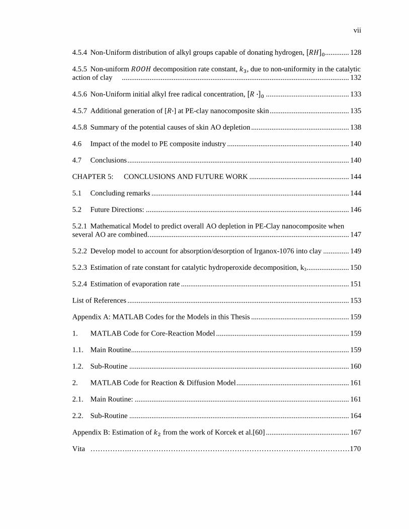
List of Tables ................................................................................................................................ viii

List of Figures ................................................................................................................................. ix

Abstract .......................................................................................................................................... xv

CHAPTER 1: INTRODUCTION ............................................................................................... 1

1.1 Background and Motivation ................................................................................................... 1

1.2 Research problem and methodology ...................................................................................... 6

1.3 Justification for the research .................................................................................................. 9

1.4 Research objectives and outline ........................................................................................... 11

1.5 Key Assumptions used in Models in this Thesis.................................................................. 13

1.6 Glossary of important terms used in this research ............................................................... 13

CHAPTER 2: CHEMICAL REACTIONS IN DEGRADATION OF POLYETHYLENE AND PE-CLAY NANOCOMPOSITES CAUSING ANTIOXIDANT DEPLETION ........................... 15

2.1 Introduction .......................................................................................................................... 15

2.2 Brief history of models describing polymer degradation and stability ................................ 15

2.3 Reactions Leading to Degradation/Stabilization of PE & PE-clay ...................................... 17

2.3.1 Initiation: Alkyl free-radical generation and their transfer .................................................. 19

2.3.2 Propagation-I: Oxidation of alkyl free-radicals and production of hydroperoxides ............ 21

2.3.3 Propagation-II: Decomposition of hydroperoxides .............................................................. 21

2.3.4 Propagation-III: Chain scission (β-Scission) ....................................................................... 23

2.3.5 Termination-I: Bimolecular combination of free-radicals ................................................... 24

2.3.6 Stabilization of free-radicals with phenolic AO ................................................................... 24

2.3.7 Termination-II: Combination of free-radicals with phenoxyl radical .................................. 27

2.4 Summary of reaction assumptions and their rate constants ................................................. 28

2.5 Reaction parameters ............................................................................................................. 30

2.6 Physical parameters determining mobility of various species within the polymeric samples31

v

2.7 Conclusions .......................................................................................................................... 34

CHAPTER 3: REACTION MODEL DESCRIBING ANTIOXIDANT DEPLETION IN SAMPLE CORE 35

3.1 Introduction .......................................................................................................................... 35

3.2 Model Equations and Assumptions ...................................................................................... 39

3.2.1 Oxygen Concentration ......................................................................................................... 39

3.2.2 Antioxidant Degradation ...................................................................................................... 40

3.2.3 Reactions of Polymer Species .............................................................................................. 41

3.3 Determination of initial concentration of alkyl groups ����� ............................................. 42

3.4 Cyclic reactions during Phase-I ........................................................................................... 44

3.5 Justification of a high hydroperoxide decomposition rate constant k�� in nanocomposites . 46

3.6 Results & Discussions .......................................................................................................... 47

3.6.1 Model Predictions for a base case ‘Comp.1010’ .................................................................. 47

3.6.2 Estimation of k�� from initial linear AO Depletion in the R.1-R.10-R.3 Reaction Cycle. ... 53

3.6.3 Analysis of Alternatives for Hydroperoxide Decomposition ............................................... 55

3.6.4 Significance of various bimolecular free-radical terminations during later times of Phase-I57

3.7 Comparison of Model to Accelerated Aging Experiments .................................................. 59

3.7.1 Neat PE with Irganox-1010 Exhibits Blooming/Exudation ................................................. 61

3.7.2 Nanocomposites with Irganox-1010 Exhibits Linear followed by Asymptotic Depletion .. 62

3.7.3 No Depletion in ‘NeatPE1076’ ............................................................................................ 67

3.7.4 Slow Core Depletion in Comp.1076 .................................................................................... 68

3.8 Additional Analysis .............................................................................................................. 71

3.8.1 Description of AO Depletion in the R.1-R.10-R.5 Reaction Cycle ..................................... 71

3.8.2 Significance of considering AO and oxygen to be present only in amorphous phase ......... 73

3.8.3 Is the assumption of constant oxygen concentration causing abrupt changes during the transition between Phase-I and Phase-II valid? ............................................................................. 76

3.8.4 Parameters determining abruptness during phase shift ........................................................ 77

vi

3.8.5 Parametric Study of Termination-II Reactions (R.15 – R.18) ............................................. 78

3.8.6 Importance of initial alkyl free radical concentration, �� ·�� ............................................... 81

3.8.7 Estimation of initial concentration of various species and influence of �� ·�� and ����� on AO depletion behavior .............................................................................................................. 82

3.9 Conclusions .......................................................................................................................... 85

CHAPTER 4: REACTION-DIFFUSION MODEL DESCRIBING ANTIOXIDANT DEPLETION THROUGHOUT THE SAMPLE DEPTH.............................................................. 88

4.1 Introduction .......................................................................................................................... 88

4.2 Model Equations and Assumptions ...................................................................................... 89

4.2.1 Oxygen Transport and Reaction ........................................................................................... 90

4.2.2 Antioxidant Transport and Degradation ............................................................................... 91

4.2.3 Reactions of Polymer Species .............................................................................................. 93

4.2.4 Numerical Method of Solution ............................................................................................. 94

4.2.5 Estimation of parameters in mathematical model to obtain agreement between model predictions and experimental features of AO depletion ................................................................. 95

4.3 Results & Discussions .......................................................................................................... 96

4.3.1 Model Predictions for a base case ‘Comp.1010’ .................................................................. 96

4.3.2 Comparison of Core-Reaction Model with Diffusion-Reaction Model ............................. 102

4.3.3 Significance of oxygen diffusion ....................................................................................... 104

4.4 Comparison of Model to Accelerated Aging Experiments ................................................ 104

4.4.1 Blooming/Exudation Observed in NeatPE1010 ................................................................. 105

4.4.2 Table-Top Profile Observed for Irganox-1010 .................................................................. 110

4.4.3 No Depletion in ‘NeatPE1076’ .......................................................................................... 114

4.4.4 No Core Depletion in ‘Comp.1076’ ................................................................................... 115

4.5 Potential Causes of Antioxidant Depleted Skin Layer ....................................................... 118

4.5.1 Effect of Clay Oriented Skin on rate of AO Depletion ...................................................... 119

4.5.2 Variable Diffusivity of O2 and AO .................................................................................... 122

4.5.3 Non-uniform oxidation rate constant, �� ........................................................................... 127

vii

4.5.4 Non-Uniform distribution of alkyl groups capable of donating hydrogen, �����............. 128

4.5.5 Non-uniform �� decomposition rate constant, ��, due to non-uniformity in the catalytic action of clay ........................................................................................................................... 132

4.5.6 Non-Uniform initial alkyl free radical concentration, �� ·�� ............................................. 133

4.5.7 Additional generation of [�·] at PE-clay nanocomposite skin ........................................... 135

4.5.8 Summary of the potential causes of skin AO depletion ..................................................... 138

4.6 Impact of the model to PE composite industry .................................................................. 140

4.7 Conclusions ........................................................................................................................ 140

CHAPTER 5: CONCLUSIONS AND FUTURE WORK ...................................................... 144

5.1 Concluding remarks ........................................................................................................... 144

5.2 Future Directions: .............................................................................................................. 146

5.2.1 Mathematical Model to predict overall AO depletion in PE-Clay nanocomposite when several AO are combined. ............................................................................................................ 147

5.2.2 Develop model to account for absorption/desorption of Irganox-1076 into clay .............. 149

5.2.3 Estimation of rate constant for catalytic hydroperoxide decomposition, k3 ....................... 150

5.2.4 Estimation of evaporation rate ........................................................................................... 151

List of References ........................................................................................................................ 153

Appendix A: MATLAB Codes for the Models in this Thesis ..................................................... 159

1. MATLAB Code for Core-Reaction Model ........................................................................ 159

1.1. Main Routine ...................................................................................................................... 159

1.2. Sub-Routine ....................................................................................................................... 160

2. MATLAB Code for Reaction & Diffusion Model ............................................................. 161

2.1. Main Routine: .................................................................................................................... 161

2.2. Sub-Routine ....................................................................................................................... 164

Appendix B: Estimation of � from the work of Korcek et al.[60] ............................................. 167

Vita …………….………………………………………………………………………………170

viii

List of Tables

Table 2.1. Types of reactions involved in degradation and stabilization of neat PE and PE-clay nanocomposites. ............................................................................................................................. 18

Table 2.2. Values of rate constants and other properties in PE as reported in the literature. ......... 30

Table 2.3. Values of various physical properties in PE as reported in the literature ..................... 32

Table 3.1. Parameters used in the model to predict AO depletion in neat PE and its clay nanocomposites. The parameters in bold font are most important parameters. For the right three columns, ‘---’ corresponds to the same parameters as in the Base Case. The values in italics were adjusted to achieve good agreement between model and experiments. ......................................... 52

Table 3.2 Bimolecular termination reactions by combination of free radicals. ............................. 57

Table 3.3. Numerical values of rates of various possible radical termination reactions in mol/cm3-s with expected rate constants and concentration data predicted from the model at about 400 days. ....................................................................................................................................................... 58

Table 3.4. Samples used in accelerated aging tests. ....................................................................... 60

Table 3.5. Values of reaction parameters used in the simplified models of Case-I and Case-II without phenoxyl reactions to predict AO depletion in Comp.1010. For the right three columns, ‘---’ corresponds to the same parameters as in Base Case. ............................................................... 66

Table 3.6. Initial concentrations of various species in amorphous phase ...................................... 74

Table 4.1. Summary of equations governing the evolution of various polymeric reactive species94

Table 4.2. Parameters used in the reaction-diffusion model in addition to the parameters listed in Table 3.1 to predict AO depletion in neat PE and its clay nanocomposites. For the right three columns, ‘---’ corresponds to the same parameters as in the Base Case. ....................................... 95

Table 4.3. Various parameters of clay ......................................................................................... 122

Table 4.4. Comparison of various hypotheses in depleting AO from skin region of PE-clay nanocomposites ............................................................................................................................ 139

ix

List of Figures

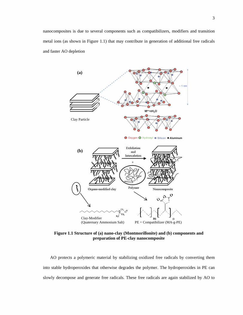
Figure 1.1 Structure of (a) nano-clay (Montmorillonite) and (b) components and preparation of PE-clay nanocomposite .................................................................................................................... 3

Figure 1.2. (a) Change in average AO (Irganox-1010) content of neat PE and PE-clay nanocomposites during accelerated aging at 85C in air. The AO content is normalized by the initial AO content of the samples; (b) AO (Irganox-1010) profiles as a function of scaled sample thickness at different aging times for PE-clay nanocomposite sample under same experimental conditions. ........................................................................................................................................ 4

Figure 1.3 (a) A typical DSC heat flow diagram showing the method of obtaining OIT; (b) Slicing technique employed to evaluate OIT profiles throughout the depth of the samples............ 8

Figure 2.1. Chemical Structure of the phenolic antioxidants (a) Irganox-1010, and (b) Irganox-1076. .............................................................................................................................................. 26

Figure 3.1. Reaction Networks for (a) neat PE and (b) PE-Clay nanocomposite. The thickness of the lines represents reaction rates; the font size of letters represents concentration; sizes of the circles represent values of rate constants. ...................................................................................... 45

Figure 3.2. (a) Depletion of phenolic group concentration, ��, as predicted by the model for typical accelerated aging conditions of PE-Clay nanocomposites. (b) Same plot in logarithmic time scale. The insets are magnification of certain sections and error in model-fitting comparison. The parameters used for this figure correspond to ‘Base Case’ of Comp.1010 in Table 3.1. Experimental data is included for comparison. .............................................................................. 48

Figure 3.3. Concentration of various polymeric reactive groups for typical accelerated aging conditions of PE-Clay nanocomposites ‘Base Case’: (a) alkyl groups ��, (b) hydroperoxides ��, (c) phenoxyl radicals � ·, (d) alkyl radicals � ·, (e) peroxide radicals � ·, and, (f) alkoxide radicals � ·. All concentrations are normalized by the initial alkyl free radical concentration, �� ·��. Inset figures display the same data with magnified vertical axis. .............. 50

Figure 3.4. Prediction for �� concentration with reaction R.0 enhanced by 104. The rest of the parameters used for this figure correspond to ‘NeatPE1010’ in Table 3.1. ................................... 56

Figure 3.5. Comparison of experimental results with model predictions for �� concentration in NeatPE1010. [19, 81] ..................................................................................................................... 60

Figure 3.6. Concentration of various polymeric reactive groups for accelerated aging conditions of NeatPE1010: (a) alkyl groups ��, (b) hydroperoxides ��, (c) phenoxyl radicals � ·, (d) alkyl radicals � ·, (e) peroxide radicals � ·, and, (f) alkoxide radicals � ·. All concentrations are normalized by the initial alkyl free radical concentration, �� ·��. Inset figures display the same data with magnified vertical axis. .................................................................................................. 61

Figure 3.7. Comparison of experimental results with model predictions for AO concentration in Comp.1010 ..................................................................................................................................... 63

x

Figure 3.8. Depletion of AO, predicted by the model without phenoxyl-radical reactions for accelerated aging conditions of Comp.1010. The parameters used for this figure correspond to different cases in Table 3.5. ........................................................................................................... 65

Figure 3.9. Concentration of various polymeric reactive groups for the cases of Figure 9: (a) alkyl radicals � ·, (b) peroxide radicals � ·, (c) alkoxide radicals � ·, and, (d) hydroperoxides ��. All concentrations are normalized by the initial alkyl free radical concentration, �� ·��. The parameters used for these predictions are presented in Table 3.5. .......................................... 65

Figure 3.10. Comparison of experimental results with model predictions for �� concentration in NeatPE1076’. ............................................................................................................................. 68

Figure 3.11. Comparison of experimental results with model predictions for �� concentration in Comp.1076. ................................................................................................................................ 70

Figure 3.12. Concentration of various polymeric reactive groups for Comp.1076: (a) alkyl groups ��, (b) hydroperoxides ��, (c) phenoxyl radicals � ·, (d) alkyl radicals � ·, (e) peroxide radicals � ·, and, (f) alkoxide radicals � ·. All concentrations are normalized by the initial alkyl free radical concentration, �� ·��. Inset figures display the same data with magnified vertical axis. ................................................................................................................................................ 70

Figure 3.13. Various reactive species in reaction cycle via R.5 in which the concentration of reactive species halve in each cycle to eventually discontinue it. .................................................. 71

Figure 3.14. Various reactive species in the reaction cycle via R.3 that continues with interruption by � · to smoothly change the slope of AO depletion. ................................................................ 73

Figure 3.15. Comparison of global and amorphous AO concentrations vs. time for the Base Case. The amorphous initial concentrations correspond to Table 3.6. .................................................... 74

Figure 3.16. Comparison of global and amorphous AO concentrations vs. time for the Base Case. This is different than Figure 3.15 because here initial � · concentration is same for both global & amorphous cases. ........................................................................................................................... 75

Figure 3.17. Comparison of AO concentrations vs. time for different crystallinities of the Base Case of Figure 3.16. ....................................................................................................................... 76

Figure 3.18. Concentration of various reactive groups at sample core (x=0) for typical accelerated aging conditions of PE-Clay nanocomposites that are evaluated using a Reaction-Diffusion model. ............................................................................................................................................ 77

Figure 3.19. Concentration of peroxide radical as a function of time for different values of k2 and k3. ................................................................................................................................................... 78

Figure 3.20. Model predictions for �� concentration for the ‘Base Case’ in Table 3.1 with varying values of rate constant, k��, that determines the rate of termination reaction between � · and � ·. ........................................................................................................................................ 79

Figure 3.21. Model predictions for �� concentration for the ‘Base Case’ in Table 3.1 with varying values of rate constant, k��, that determines the rate of termination reaction between � · and � ·. ............................................................................................................................. 80

xi

Figure 3.22. Model predictions for �� concentration for the ‘Base Case’ in Table 3.1 with varying values of rate constant, k��, that determines the rate of termination reaction between � · and � ·. ........................................................................................................................................ 80

Figure 3.23. Model predictions for �� concentration for the ‘Base Case’ in Table 3.1 with varying values of rate constant, k��, that determines the rate of bimolecular termination reaction within � ·. .................................................................................................................................... 81

Figure 3.24. Model predictions for �� concentration for the ‘Base Case’ in Table 3.1 with varying values of initial alkyl free radical concentration, �� ·��, keeping ����� = 0. ............. 82

Figure 3.25. Predictions for �� concentration vs. time during processing of ‘Comp.1010’. ..... 83

Figure 3.26. Concentration of various polymeric reactive groups during processing of Comp.1010 ....................................................................................................................................................... 84

Figure 3.27. Model predictions for �� concentration for the ‘Base Case’ in Table 3.1 with varying values of initial hydroperoxide concentration, �����, keeping �� ·�� = 0. ................. 85

Figure 4.1. Schematic diagram of PE (a), and PE-clay (b) samples showing one-dimensional coordinate system. The diameter of spherulites in PE and length of clay particles are in the same order. The clay particles orient themselves along the edges of the samples. ................................. 90

Figure 4.2. Concentration profiles of (a) O2 and (b) ��, predicted by the model for typical accelerated aging conditions of Comp.1010. The parameters used for this figure correspond to ‘Base Case’ in Table 4.2. ............................................................................................................... 96

Figure 4.3. Concentration profiles of various polymeric species for typical accelerated aging conditions of PE-Clay nanocomposites ‘Base Case’ for same times as in Figure 4.3. .................. 97

Figure 4.4. Concentration profiles of �� for the cases of (a) no evaporation, (b) no reaction, and (c) 10 times faster �� diffusion than typical case of Figure 4.2(b). ........................................... 97

Figure 4.5. Total Oxygen and �� during first 90 days for typical aging conditions of the ‘Base Case’. ............................................................................................................................................. 99

Figure 4.6. Concentration profiles of various reactive species for typical accelerated aging conditions of PE-Clay nanocomposites ‘Base Case’ during initial transient. .............................. 100

Figure 4.7. Depth of �� rich layer developed in presence of �� (a) and during absence of �� when actual PE degradation starts (b)................................................................................. 102

Figure 4.8. Comparison of concentrations of various reactive groups at sample core for typical accelerated aging conditions of PE-Clay nanocomposites ‘Base Case’ obtained by Core-Reaction Model and by Diffusion-Reaction Model: (a) oxygen 2, (b) hydroperoxides ��, (c) phenoxyl radicals � ·, (d) alkyl radicals � ·, (e) peroxide radicals � ·, and, (f) alkoxy radicals � ·. All concentrations are normalized by the initial alkyl free radical concentration, �� ·��. . 103

Figure 4.9. Parametric study of the effect of kb on the growth of the bloomed film thickness, h (dimensionless). The predicted thickness profile is insensitive to kb when kb is greater than 10 s-

1. ................................................................................................................................................... 107

xii

Figure 4.10. Comparison of the model predictions with experimental results for: (a) NeatPE1010 under forced air convection; (b) NeatPE1010 under stagnant N2 condition. The solid lines represent experimental data and the dashed lines represent model predictions for each experimental slice. The dotted smooth lines are the model predictions for precise �� distribution throughout the sample depth..................................................................................... 109

Figure 4.11. Comparison of the model predictions with experimental results for: (a) Comp.1010 under forced air condition; (b) Comp.1010 under slow air convection; (c) Comp.1010 under stagnant N2 condition. The solid lines represent experimental data and the dashed lines represent model predictions for each experimental slice. The dotted smooth lines are the model predictions for precise �� distribution throughout the sample depth. ........................................................ 111

Figure 4.12. Depletion of total AO content and growth of depth of AO depleted layer with time for ‘Comp. 1010’ under forced-air condition: (a) Predictions by Model, (b) Experimental observations. ................................................................................................................................ 112

Figure 4.13. Comparison of the model predictions with experimental results for NeatPE1076 under forced air convection. The solid lines represent experimental data and the dashed lines represent model predictions for each experimental slice. The dotted smooth lines are the model predictions for precise �� distribution throughout the sample depth. ...................................... 115

Figure 4.14. Comparison of the model predictions with experimental results for: (a) Comp1076 under forced air convection; (b) Comp1076 under stagnant N2 condition. The solid lines represent experimental data and the dashed lines represent model predictions for each experimental slice. The dotted smooth lines are the model predictions for precise �� distribution throughout the sample depth. ............................................................................................................................... 117

Figure 4.15. Depletion of total AO content and growth of depth of AO depleted layer with time for ‘Comp. 1076’ under forced-air condition: (a) Predictions by Model, (b) Experimental observations. ................................................................................................................................ 118

Figure 4.16. Schematic diagrams of Comp.1010 samples showing the technique used to measure: (a) OIT profiles through sample depth from clay oriented surface to interior of the samples; and (b) OIT profiles from surface to core for samples with skin layers removed before aging process. [21] ............................................................................................................................................... 120

Figure 4.17. Comparison of the model predictions with experimental results utilizing the slicing technique of Figure 4.16 for: (a) Comp.1010 with skin layer under forced air condition with evaporation rate ��� � � = 2 ×10-8 cm/s (b) Comp.1010 without skin layer under forced air condition with evaporation rate ��� � � = 10-9 cm/s. ................................................................. 121

Figure 4.18. Ratio of diffusivity of mobile molecules in the PE-clay nanocomposites to their diffusivity in neat PE as a function of clay orientation order parameter �. Here the aspect ratio of nano-clay, � �⁄ , is considered to be 60.5 and other parameters are listed in Table 4.3.............. 123

Figure 4.19. Distribution of: (a) diffusivity; (b) oxygen; and (c) phenolic groups in AO throughout the depth of Comp.1010 under the conditions of hyperbolic tangent distribution of diffusion in Equation 4.19 and evaporation rate 5 times more than NeatPE1076 (��� � � = 10-9 cm/s). Here �=0.6, �=10, ��� �⁄ =0.6 and �� �⁄ =0.93. ........................................................... 125

xiii

Figure 4.20. Distribution of: (a) diffusivity; (b) oxygen; and (c) phenolic groups in AO throughout the depth of Comp.1010 under the conditions of Figure 4.19 with diffusivity at skin 100 times lower than at core. ....................................................................................................... 126

Figure 4.21. Distribution of: (a) diffusivity; (b) oxygen; and (c) phenolic groups in AO throughout the depth of Comp.1010 under the conditions of Figure 4.19 with diffusivity at skin 1000 times lower than at core. ..................................................................................................... 126

Figure 4.22. Distribution of: (a) oxidation constant; (b) oxygen; and (c) phenolic groups in AO throughout the depth of Comp.1010 under the conditions of the base-case with modified �� and evaporation rate of ��� � � = 10-9 cm/s. ..................................................................................... 128

Figure 4.23. Distribution of phenolic groups in AO throughout the depth of Comp.1010 under the conditions of Figure 4.22 with: (a) ��(skin) = 100 × ��(core), (b) uniform ��, and (c) ��(core) = 0.1 × ��(skin). .............................................................................................................................. 128

Figure 4.24. Distribution of: (a) �����; (b) oxygen; and (c) phenolic groups in AO throughout the depth of Comp.1010 under the conditions of the base-case with modified ����� and evaporation rate of ��� � � = 10-9 cm/s. ......................................................................................................... 130

Figure 4.25. Concentration profiles of various polymeric species under the conditions of Figure 4.24. Inset figures display the same data with magnified vertical axis. ....................................... 131

Figure 4.26. Distribution of: (a) �����; (b) oxygen; and (c) phenolic groups in AO throughout the depth of Comp.1010 under the conditions of Figure 4.24 with ����� = 10-4 mol/cm3 at core in the core (x < 0.7) and ����� = 15 × 10-3 mol/cm3 in the skin. In the middle figure (b), the circled points and arrow shows the time progression of O2 profiles. ...................................................... 131

Figure 4.27. Distribution of: (a) �����; (b) oxygen; and (c) phenolic groups in AO throughout the depth of Comp.1010 under the conditions of Figure 4.24 with ����� = 10-4 mol/cm3 at core in the core (x < 0.7) and ����� = 15 × 10-3 mol/cm3 in the skin. .......................................................... 132

Figure 4.28. Distribution of: (a) �� decomposition constant; (b) oxygen; and (c) phenolic groups in AO throughout the depth of Comp.1010 under the conditions of base-case with modified ��� and evaporation rate of ��� � � = 10-9 cm/s. .......................................................... 133

Figure 4.29. Distribution of: (a) alkyl free radical; (b) oxygen; and (c) phenoxyl groups in AO throughout the depth of Comp.1010. Here the initial [R*] at skin is 10 time higher than at core. ..................................................................................................................................................... 134

Figure 4.30. Distribution of: (a) alkyl free radical; (b) oxygen; and (c) phenoxyl groups in AO throughout the depth of Comp.1010. Here the initial [R*] at skin is 600 times higher than at core. ..................................................................................................................................................... 134

Figure 4.31. Distribution of: (a) oxygen; and (b) phenolic groups in AO throughout the depth of Comp.1010 under the conditions of additional generation of �· at ! > 0.7 with "# = 3.9×10-14 cm3/mol-s in Equation 4.20 and surface AO evaporation rate of ��� � � = 10-9 cm/s. .............. 136

Figure 4.32. Concentration profiles of various polymeric species under the conditions of Figure 4.31. Inset figures display the same data with magnified vertical axis. ....................................... 137

xiv

Figure 4.33. Distribution of phenolic groups in AO throughout the depth of Comp.1010 under the conditions of Figure 4.31 with (a) "# = 3.9×10-15 cm3/mol-s and (b) "# = 3.9×10-13 cm3/mol-s. 138

Figure 5.1 Chemical structure of Irgafos-168 .............................................................................. 148

Figure 5.2 OIT verses aging time for PE-clay nanocomposites with Irganox-1076 .................... 149

xv

Abstract

Mathematical Models to Describe Antioxidant Depletion in Polyethylene-Clay Nanocomposites under Thermal Aging

Iftekhar Ahmad Richard Cairncross, Ph.D.

Antioxidants are typically added to polyethylene to extend its durability, and recently clay

nanoparticles have been blended into polyethylene to improve mechanical properties. However,

the clay nanoparticles also accelerate the rate of antioxidant depletion in polyethylene. This thesis

presents mathematical models that describe the underlying mechanisms of antioxidant (hindered-

phenol) depletion and predict experimentally-measured antioxidant profiles in polyethylene-clay

nanocomposites.

The mathematical models use a reaction kinetic scheme that includes free radical initiation

and propagation reactions, antioxidant stabilization reactions and free radical termination

reactions. In the model, alkyl free radicals oxidize rapidly. The role of antioxidants is to stabilize

the oxidized free radicals to hydroperoxides, and interrupt propagation reactions. However, in

nanocomposites, continuous depletion of antioxidant is caused by the clay acting as a catalyst to

decompose hydroperoxides and regenerate alkyl free radicals. This cyclic hydroperoxide

generation and decomposition leads to much faster antioxidant depletion in polyethylene

nanocomposites. Phenoxyl radicals of antioxidants generated by stabilization reactions contribute

to terminate polymeric free radicals and limit their accumulation.

The model also describes diffusion of antioxidant and oxygen within the samples and loss of

antioxidant by evaporation or blooming to the surface of neat polyethylene. In nanocomposite

samples there are two zones of antioxidant depletion: a ‘flat core zone’ and ‘depleted skin zone’.

In the flat core zone antioxidant depletion is slower and uniform, and in the depleted skin zone,

xvi

antioxidant depletes more rapidly to produce a skin layer which is void of active antioxidant. The

diffusion-reaction model describes this by combining several factors such as variable diffusivity

caused by clay orientation at skin and additional generation of alkyl free radicals at the skin layer.

The model also predicts antioxidant depletion profiles for a number of different experimental

conditions including aging in air or inert atmosphere that cause different profiles of antioxidant

concentration.

xvii

1

CHAPTER 1: INTRODUCTION

Antioxidants are typically added to polyethylene to extend its durability, and recently clay

has been blended into polyethylene to improve mechanical properties. However, clay

nanoparticles can also accelerate the rate of antioxidant depletion in polyethylene leading to

shorter product life. This has challenged commercialization of PE-clay nanocomposites. In this

thesis, mathematical models have been utilized to describe the causes of the accelerated

antioxidant depletion.

1.1 Background and Motivation

The global production of polyethylene (PE) is about 100 million tons per year and is growing

almost 5% annually[1]. Several advantages of PE over other plastics/metals include low cost,

good processability, non-toxicity and good recycling performance. However, PE is inferior to

other plastics/metals in mechanical properties. Many properties of PE, such as modulus[2-6],

barrier properties[7-10], and even strength[11] are improved by adding clay and carefully

processing it to form nanocomposites. Figure 1.1(a) shows the chemical structure of clay and

Figure 1.1(b) shows a schematic of the components in PE-clay nanocomposites and how they are

dispersed during processing. The type of clay widely used with PE is montmorillonite, which is a

layered alumino-silicate of roughly 1 nm thick negatively-charged silica layers separated by metal

cations. To achieve effective dispersion of clay in a hydrophobic non-polar PE matrix, the cations

in clay are partially exchanged with organic cation surfactant (quaternary-alkyl-ammonium salt)

[12]. In addition, a compatibilizing agent such as maleic-anhydride-grafted-PE creates polarity in

PE matrix and enhances interaction with modified clay. These modifications enable PE molecules

to diffuse between clay layers to achieve intercalated and exfoliated morphologies as shown in

Figure 1.1(b).

2

Despite a large amount of research on material properties and processing techniques of PE

nanocomposites, the long-term performance is still poorly understood. Long-term degradation of

PE properties is primarily due to environmental oxidative degradation which is inhibited by

antioxidants (AO). However in nanocomposites, AO proves unsuccessful in inhibiting the

degradation for long time because the clay catalyzes some degradation reactions in polyethylene.

In this thesis, two new models describing AO depletion are used to explore mechanisms by which

the presence of clay leads to accelerated AO depletion.

Polymers degrade mainly due to oxidative reaction with free radicals. Free radicals in PE are

generated by breakage of chemical bonds which occurs faster during processing at high

temperature and at much slower rate at 85°C. Atmospheric oxygen reacts with these free radicals

to propagate degradation. AO protects degradation by reacting with oxidized free radicals and

converting them to stable hydroperoxides. After the AO is depleted, the PE material is no longer

protected from oxidized free radicals. Therefore, degradation of PE can be divided into two broad

phases: (Phase-I) ‘AO-protected’ phase when AO protects PE from degradation, and (Phase-II)

‘PE-degradation’ phase when AO no longer protects PE, and chain reactions lead to increases in

free radical concentrations.

In presence of clay, AO depletion and polymer degradation has been found to be

accelerated[13-19]. Figure 1.2 shows typical AO (Irganox-1010) depletion in PE and PE-clay

nanocomposite and distribution of AO throughout the nanocomposite sample from data provided

by collaborators on this research. In Figure 1.2(a), the average AO does not deplete in neat PE

and provides a long term protection from oxidative degradation. But in case of the

nanocomposite, Figure 1.2 shows that the average AO concentration reaches 50% of its initial

amount in about 170 days of aging at 85°C. In another work[20], the overall oxidative

polypropylene degradation of nanocomposites is reported to be about 4 times faster than pure

polymer. In the past it has been postulated that accelerated AO depletion in PE-clay

3

nanocomposites is due to several components such as compatibilizers, modifiers and transition

metal ions (as shown in Figure 1.1) that may contribute in generation of additional free radicals

and faster AO depletion

Figure 1.1 Structure of (a) nano-clay (Montmorillonite) and (b) components and preparation of PE-clay nanocomposite

AO protects a polymeric material by stabilizing oxidized free radicals by converting them

into stable hydroperoxides that otherwise degrades the polymer. The hydroperoxides in PE can

slowly decompose and generate free radicals. These free radicals are again stabilized by AO to

(b)

PE + Compatibilizer (MA-g-PE) Clay-Modifier (Quaternary Ammonium Salt)

(a)

Clay Particle

regenerate the hydroperox

hydroperoxides leads to

decomposition can be catalyzed causing

Figure 1.2. (a) Change in average nanocomposites during accelerated aging at 85C in air

the initial AO content of the samples; (b) AO (Irganoxsample thickness at different aging times for PE

Figure 1.2(b) shows depletion profiles of AO (Irganox

clay nanocomposite sample aged at 85

the depletion behaviors are different.

uniform while in the ‘skin’ layer almost all AO is quickly depleted.

a flat core depletion results in a ‘table

explained by the degradation mechanism explained above, but mechanism explaining additional

loss of AO at skin is required in order to completely deplete AO. Several mechanisms

proposed in this thesis for the skin

• Diffusion of AO to sample surface where it can evaporate;

0

0.2

0.4

0.6

0.8

1

0 200 400

[AO

]/[A

O]

0

Time, days

(a)

regenerate the hydroperoxides in a cycle. This cyclic decomposition and

leads to slow depletion of AO. In presence of clay, this hydroperoxide

decomposition can be catalyzed causing accelerated AO depletion in the nanocomposites.

Change in average AO (Irganox-1010) content of neat PE and PEduring accelerated aging at 85C in air. The AO content is normalized by

content of the samples; (b) AO (Irganox-1010) profiles as a function of scaled sample thickness at different aging times for PE-clay nanocomposite sample

experimental conditions.

(b) shows depletion profiles of AO (Irganox-1010) throughout the depth of a PE

clay nanocomposite sample aged at 85°C. The AO distributions show two different regions where

iors are different. Inside of the sample, in the ‘core’ region

while in the ‘skin’ layer almost all AO is quickly depleted. A sharp depletion at skin and

a flat core depletion results in a ‘table-top’-like AO profile. The core AO d

explained by the degradation mechanism explained above, but mechanism explaining additional

loss of AO at skin is required in order to completely deplete AO. Several mechanisms

proposed in this thesis for the skin-core gradient, the most important of which are

Diffusion of AO to sample surface where it can evaporate;

600 800

Time, days

PE-Clay-1010

Neat PE

0

0.2

0.4

0.6

0.8

1

-1 -0.5 0

[AO

]/[A

O]0

Scaled distance

0 day 30 days120 days 181 days

Core Ski

n

(b)

4

decomposition and generation

In presence of clay, this hydroperoxide

nanocomposites.

PE and PE-clay

The AO content is normalized by 1010) profiles as a function of scaled

clay nanocomposite sample under same

1010) throughout the depth of a PE-

The AO distributions show two different regions where

’ region, AO depletion is

A sharp depletion at skin and

The core AO depletion can be

explained by the degradation mechanism explained above, but mechanism explaining additional

loss of AO at skin is required in order to completely deplete AO. Several mechanisms have been

he most important of which are:

0.5 1

Scaled distance

30 days 62 days181 days 445 days

Ski

n

5

• Spatial differences in diffusivity;

• Higher number of weak C-H bonds at skin

• Additional generation of free radicals at the skin.

AO can deplete slowly by diffusing to the sample surface where AO can evaporate. This is

significant for small AO molecules with comparatively higher volatility. Also, in injection

molded samples, the clay platelets are more highly oriented at sample surfaces than in the center

creating a morphological inhomogeneity through the sample depth[21]. This morphological

inhomogeneity can cause spatial differences in the diffusivities of the reactive species and might

also cause inhomogeneity in their reaction parameters. Another cause of AO depletion can be due

to strained PE molecules in the skin leading to C-C bond scission and generation of submicron-

cracks. These strains can be developed due to clay orientation and quenching of the

nanocomposite surface while molding or due to higher defects in PE molecule in the skin. An

individual submicron-crack is formed by the rupture of numerous C-C bonds in PE[22]. These

ruptures generate alkyl free radicals that can generate allyl groups or are oxidized followed by

AO stabilization. The allyl groups have weak C-H bonds and can propagate the degradation

reactions.

Mathematical modeling and computer simulation of the PE-clay degradation can predict

experimental AO depletion features and give insight to identify significance of various

degradation and stabilization reactions. Various hypotheses for accelerated AO depletion at core

of the nanocomposites and for complete AO depletion at skin can be evaluated by utilizing

mathematical models. The models can predict experimental features od AO depletion in matters

of minutes/hours, the experiments for which would require several years. Although there is some

prior work in the literature on modeling AO diffusion and depletion in PE & PP, there are not any

published models of AO depletion in PE-clay nanocomposites.

6

1.2 Research problem and methodology

The research problem addressed in this research is:

What causes severe antioxidant depletion in PE-clay nanocomposites?

The results in this thesis show that accelerated depletion of AO is brought about by the catalytic

effect of clay in decomposing the hydroperoxides which are quite stable in neat PE. The higher

rate of AO depletion at skin of the nanocomposite samples is due to the additional loss of AO and

slow diffusion of AO from the sample core. The additional loss can be due to combination of

several factors including surface evaporation and morphological inhomogeneity.

Although some literature does exist to describe polymer degradation and antioxidant

depletion in polymer-clay nanocomposites, detailed kinetic models have not been published.

Therefore, the first stage of this research is detailed study of reaction kinetics in oxidative thermal

degradation of PE. The literature proposes several hypotheses for accelerated AO depletion in

PE-clay nanocomposites that have not been rigorously evaluated. Because of the interdisciplinary

nature of the work, the findings of this research were often discussed between our collaborators in

Civil Engineering & Materials Science Engineering Departments at Drexel University. This

created opportunity to learn from other disciplines promoted collegiality. The collaborators

helped with the thermal degradation experiments and measurement of AO depletion of various

samples utilizing OIT technique. These experimental OIT profiles guided the development of the

models in this thesis. A core-reaction model is developed that gives details of oxidative

degradation mechanism and AO depletion in the bulk core of the nanocomposite samples. Here

‘core-reaction’ model implies a lumped-parameter approach where spatial gradients are ignored.

In order to understand the AO depletion throughout the depth of the samples, a diffusion-reaction

model also includes effects of diffusion of AO and O2 coupled with the degradation and

stabilization reactions.

7

It has been postulated in the literature that PE-clay nanocomposites contain several

components that could contribute to generation of additional free radicals and faster AO

depletion. The organic modifiers (alkyl ammonium ions) and compatibilizers enhance interaction

between clay and PE, but they might also have a negative effect on processing and durability[15,

16] of PE products. During PE melt processing, thermal decomposition of the organic modifier is

known to be enhanced by the so-called Hoffman elimination[18]. Also, the presence of transition

metal ions as impurities in the clay can catalyze the degradation reactions[14].

In order to evaluate these hypotheses, a mathematical model had to be developed with the

help of experimental results. Consumption of AO in neat PE and its nanocomposite under normal

atmospheric conditions may take several decades; therefore, our collaborators used accelerated

thermal aging in the experimental study[19]. Here ‘neat PE’ refers to PE with 2wt% maleic-

anhydride grafted PE (MA-g-PE). Samples were held at 85°C in a circulated air atmosphere, and

AO concentrations in aged samples were determined by measuring ‘oxidation induction times’

(OIT).

OIT is an indirect method of measuring AO concentration in a DSC instrument. Figure 1.3(a)

shows a DSC heat flow curve with time. The first part shows melting of nanocomposite sample at

200 ˚C under N2 atm. From this time onwards oxygen flow starts and initiates oxidative reactions.

Propagation of degradation is inhibited by AO present in the sample. When all AOs are

consumed, degradation reactions propagate producing an exothermic peak. The time duration

between start of oxygen flow until the onset of exothermic peak is referred to as OIT which is

linearly proportional to the phenolic AO content in the un-aged samples.

Figure 1.3(b) depicts the method used to determine AO concentration as a function of

distance. A thick sample is sliced into several layers which were each individually subjected to

OIT test. OIT of these slices provided experimental AO distribution profile throughout the sample

depth such as shown in Figure 1.2(b).

8

Figure 1.3 (a) A typical DSC heat flow diagram showing the method of obtaining OIT; (b) Slicing technique employed to evaluate OIT profiles throughout the depth of the samples.

Although OIT is an indirect measure of active AO concentration present in a polymeric

sample, OIT and AO concentration are linearly proportional for the AOs (Irganox-1010, and

Irganox-1076) discussed in this research[23-25]. There might be some deviation from this linear

relationship for aged PE and PE-clay nanocomposites as discussed by Richaud[26], but in this

thesis the relation is treated as linear for all experimental analysis.

Degradation of stabilized and unstabilized PE has been modeled by several researchers in the

1980s, which is reviewed in Chapter 3. The published models have a number of weaknesses

including many models that assumed constant initiation rate that were not well justified and

steady state assumption of various free radical species. These assumptions invalidate predictions

of long term thermal degradation behavior. In addition, although there is some prior work in the

literature on modeling AO diffusion and depletion in PE & PP, there are not any published

models of AO depletion in PE-clay nanocomposites. Therefore, this thesis presents two models

that predict experimental AO depletion with improved assumptions and evaluates several

hypotheses to evaluate the cause of accelerated AO depletion. In the models, fast hydroperoxide

(��) decomposition is found to be the potential cause of accelerated AO depletion. However,

(b)

Sample bar

t1

(a) E

xo

the

rmE

nd

oth

erm

N2

at 0.035 MPa

OxidativeReaction

Isothermal at 200oCunder O2 at 0.035

MPa

OIT

Time (min)

Heat Flow(W/g)

9

none of the past postulates for fast �� decomposition are able to predict the experimental

features. Therefore, a new catalytic reaction mechanism has been proposed in this work that

predicts the experimental features. A diffusion and reaction model is also presented that shows

how surface AO evaporation and morphological inhomogeneity can cause even further loss of

AO from the skin layer of the nanocomposite samples.

Because �� decomposition catalyzed by clay limits the effectiveness of AO at stabilizing

all free radicals, this thesis concludes that for long service lifetime of the nanocomposites, a

transition of research is needed to develop antioxidants that stabilize free radicals without

generating �� or that stabilize ��. One way to stabilize without generating �� is to

stabilize �· itself before it oxidizes but then the challenge is to develop highly reactive AOs. To

stabilize ��, hydroperoxide scavengers like sulphite/phosphite antioxidant is required. It has

been found in this research that antioxidants that have higher phenoxyl termination rates can

provide better durability to the nanocomposites. With higher phenoxyl termination rate Irganox

1076 is more effective antioxidant for polyethylene nanocomposites than Irganox 1010. Also, an

antioxidant with high solubility in PE allows higher initial dosing of AO leading to higher

durability.

1.3 Justification for the research

It has been found in the past decades that adding 1-3 % of clay can significantly improve PE

mechanical properties. However, accelerated AO depletion in presence of clay has challenged

commercialization of PE-clay nanocomposites. Although there is a substantial amount of

literature measuring AO depletion in pure PE, the literature on AO depletion in PE-clay

nanocomposite is minimal. The postulates made in the past for potential accelerated AO depletion

in nanocomposites are poorly understood and hypotheses for the accelerated depletion have not

been thoroughly evaluated. In addition, there are no models reported in the literature to describe

AO distribution in PE-clay nanocomposites. Mathematical modeling and computer simulation of

10

the nanocomposite degradation assist developing insight into underlying mechanisms and

evaluating proposed mechanisms.

Most of the early works on PE degradation[27, 28] reported in literature considered empirical

degradation equation to fit experimental results. Most of the experiments were conducted under

IR irradiation[28-30] where the degradation is very fast. Short term experiments under high

irradiation rate or high temperature often lead to conclude that AO depletes linearly with time

which is not true in the long run. Experiments on long term thermal degradation at low

temperatures of about 85°C is minimal. Thin films or excess oxygen were considered to avoid

diffusional effects. In early 1980s kinetic models were considered in order to logically explain PE

degradation and AO depletion. But most of them assumed a constant free radical initiation rate

which is not justified for thermal degradation. Moreover, the hydroperoxide and other free

radicals would be assumed to be at steady state that simplifies the kinetic model. Since such

assumptions are questionable, this research presents a reaction scheme with limited and justified

assumptions. The parameters for various reactions have been estimated from the literature.

Although AO depletion has been modeled in the past in pure PE, but there is no work

reported in literature that models accelerated AO depletion in PE-clay nanocomposites. Several

postulations have been made in the past for the experimentally observed accelerated AO

depletion such as oxidation of PE molecules and accelerated hydroperoxide decomposition due to

catalytic effect of transition metal ions in clay. In this work, these speculations were evaluated by

the model giving a deeper insight into various possibilities for the accelerated AO depletion.

Manufactured plastics parts are sometimes expected to withstand moderate heat and long

term storage or long term usage. Therefore, it is a requirement that AO is retained during the

service lifetime of a plastic product to ensure protection from oxidative degradation. So,

development of a model that can predict AO durability is highly desired by PE composite

industry.

11

This research is very useful in understanding the underlying mechanisms leading to sharp AO

depletion. This understanding would guide further research in enhancing the durability of

polymer-clay nanocomposites.

1.4 Research objectives and outline

This thesis presents two new models of AO depletion in PE and PE-clay nanocomposites: (1)

a core reaction model to describe AO depletion in the bulk core of the nanocomposite samples,

and (2) a diffusion and reaction model to describe AO depletion profiles throughout the sample

depth. Both models use the same set of chemical reactions leading to AO depletion in PE and PE-

clay nanocomposites that are presented in Chapter 2. Then the core model is developed in

Chapter 3 using experimentally measured OIT values at the center of the samples (core). Chapter

4 presents the diffusion-reaction model in which both oxygen and AO diffuse within the thickness

of the samples leading to non-uniform AO profiles. The specific research objectives of this thesis

are summarized below in the following list:

The research objectives of this work are, therefore, summarized below:

1. Develop kinetic reaction scheme for Neat PE and PE-Clay nanocomposite (Chapter 2):

o Review literature of PE degradation and stabilization to catalog reactions

accounting for free radical generation, oxidation of free radicals, hydroperoxide

decomposition, termination and stabilization

o Review mechanisms proposed by researchers to explain faster AO depletion in

PE-Clay nanocomposites than in neat PE

o Review Literature to determine reaction parameters for PE

2. Develop a lumped-parameter reaction model to predict core-AO depletion (Chapter 3)

12

o Use core-reaction model to predict experimental core AO depletion, estimate

model parameters to improve model-experiment agreement, and evaluate the

estimated parameter values

o Evaluate various postulates reported in literature accounting for accelerated core-

AO depletion in some PE-clay nanocomposites

� Higher hydroperoxide decomposition rate by transition metals [17]

� Higher initial free radical concentration [18]

� Higher hydroperoxide decomposition rate by quaternary ammonium

(proposed in this thesis)

o Perform parametric studies with the core-reaction model to improve knowledge

of reaction mechanisms that lead to different observed AO depletion versus time

3. Develop reaction & diffusion model to predict AO depletion throughout the sample

thickness (Chapter 4)

o Use model and experimental comparison to explain reaction and diffusion

mechanisms of AO depletion throughout the depth of samples

o Evaluate the hypothesis that diffusion of oxygen leads to observed gradients in

AO concentration.

o Modify boundary conditions to predict ‘blooming’ at sample surface in neat PE.

o Evaluate various hypotheses in predicting accelerated AO depletion at skin layer

� Physical loss via evaporation

� Morphological variation due to clay orientation and or clay density

gradient

� Chemical loss due to initial free radical gradient or alkyl group gradient

� Strained PE molecule causing submicron-crack

13

1.5 Key Assumptions used in Models in this Thesis

The models presented in this thesis have been derived to predict specific types of experiments

related to AO depletion. Some of the key assumptions are listed below that were used to guide

development of the models in this thesis.

Homogeneous Matrix: Homogeneous Matrix has been considered since no significant

change in crystallinity is observed in the samples.

Global Concentration: Global Concentration is considered for all reactive species including

the AOs. This assumption is valid when all the degradation reactions are occurring in the

amorphous phase.

Immobile polymeric species: All polymeric species are assumed to be immobile because

their diffusivities can be about 100 million times lower than AO diffusivity.

Precision of end products: This work has ignored the precision of stable end products of

degradation that can predict the amount of carbonyl and hydroxyl groups, and other small

molecular weight hydrocarbons. This is because the goal of this work is to predict AO depletion

and understand its underlying mechanism that pertains to Phase-I reactions only.

Linear relation of OIT with AO concentration: OIT is considered to be linearly proportional

to AO concentration. This is mostly true for un-aged PE, and could be challenged for aged and

nanocomposite samples [26]. In this thesis, OIT is assumed to be linearly proportional to AO

concentration for both aged and un-aged samples.

1.6 Glossary of important terms used in this research

Some technical terms adopted by researchers in PE degradation and stabilization are not

uniform. Therefore, this section clarifies and interprets several important terms used in

nanocomposite literature that are adopted in this thesis.

14

Alkoxide and Peroxide radicals: Alkoxide groups in PE have one oxygen molecule with a

free radical, and peroxide groups in PE have two oxygen molecules with a free radical. They are

also termed as Alkoxy and Peroxy radicals respectively

AO: Antioxidant molecule that may contain both phenolic group (��) and phenoxyl

radicals (�·). $%&: A phenol group in AO molecule capable to trapping a free radical.

$%···· : A phenoxyl group in AO that has a trapped free radical that can terminate another free

radical or even propagate degradation reactions.

Irganox-1010: [3-[3-(3,5-ditert-butyl-4-hydroxyphenyl)propanoyloxy]-2,2-bis[3-(3,5-ditert-

butyl-4-hydroxyphenyl)propanoyloxymethyl]propyl] 3-(3,5-ditert-butyl-4-

hydroxyphenyl)propanoate – a commercial antioxidant produced by BASF.

Irganox-1076: Octadecyl 3-(3,5-di-tert-butyl-4-hydroxyphenyl)propionate – a commercial

antioxidant produced by BASF.

MA-g-PE: Maleic-anhydride grafted polyethylene

Nanoclay: Organically modified clay (montmorillonite in this case) that can

intercalate/exfoliate in polymer matrix to form nanocomposite.

Nanocomposites: A composite where the solid filler is dispersed into the medium in such a

way that at least one of the spatial dimensions of the particles is less than 100 nm.

Neat polyethylene: Pure polyethylene blended with a compatibilizer – MA-g-PE (maleic-

anhydride grafted PE) in this case

Pure polyethylene: Raw polyethylene without any additive

Phase-I: Polymer oxidation and AO depletion phase during which AO is still active in

protecting the polymer.

Phase-II: Actual polymer degradation phase that starts when all AO is depleted.

15

CHAPTER 2: CHEMICAL REACTIONS IN DEGRADATION OF POLYETHYLENE AND PE-CLAY NANOCOMPOSITES CAUSING

ANTIOXIDANT DEPLETION

2.1 Introduction

The primary cause of AO depletion is by reaction with peroxide free radicals. In the presence

of oxygen, alkyl free radicals on polyethylene react to form peroxide free radicals, which can lead

to a chain of further free radical reactions, causing degradation in mechanical properties. AO

interrupts this chain reaction by converting peroxide free radicals into hydroperoxides that are

stable in neat PE.

The following sections summarize the degradation reactions of PE and PE-clay

nanocomposites and the reactions are all listed in Table 1. Degradation begins with an initiation

step which generates alkyl free radicals. Free radicals then react through propagation, chain

scission and termination reactions.

2.2 Brief history of models describing polymer degradation and stability

Researchers started using models to describe polymer degradation in the mid-20th century.

Initially, basic chemical reactions of free radical oxidation, propagation and termination were

considered to predict experimental evolution of carbonyl groups and oxygen uptake

measurements in unstabilized polymers. Polymer samples were exposed to high heat or high

irradiation to achieve quick degradation. Often, thin films and excess oxygen were used to avoid

diffusional effects. Around 1980s several researchers attempted to produce better kinetic models

of polymer degradation, and stabilization reactions were also introduced. In most of these works,

constant free radicals initiation and steady state hydroperoxide concentration were assumed that

are not justified for long term thermal degradation.

16

The earliest work on developing a kinetic model for polymer degradation dates back to 1950

when Tobolsky et al.[31] used auto-oxidation reaction schemes with hydroperoxide

decomposition and generation cycle to determine oxygen and hydroperoxide concentration in

vulcanized natural rubber under irradiation. Similar kinetic schemes for thermal degradation of

polyolefins were studied by other researchers such as Notley[27] in 1961, who used oxygen

uptake to measure PE degradation reactions, and Stivala et al.[28] in 1962, who used infra-red

spectroscopy to measure PP degradation reactions. Most of these early works considered thin

films or excess oxygen to avoid diffusional effects of oxygen. Among the early works that

included oxygen diffusion is that of Iring et al.[32] in 1975 and Seguchi et al. in 1981[30]. Iring

found diffusion of oxygen to limit oxidative degradation at 157 °C and considered an empirical

degradation rather than a detailed kinetic reaction scheme. Seguchi used oxygen diffusion and

reaction model to determine oxygen penetration under relatively high irradiation rate. Most of

these early models relied on the assumption of a constant initiation rate, which could not predict

long term thermal degradation. Therefore, authors like Gugumus[33, 34] derived heterogeneous

kinetic models where the depth of oxidation is time dependent. With an increasing body of

experimental results (using infra-red spectroscopy, and thermo gravimetric analysis, etc.), the

kinetic schemes of unstabilized polymers were improved by several researchers like Gugumus,

Zweifel, Colin etc. Experiments were conducted in solid state polymers rather than on polymer

melts or solutions to finds the rates of formation of carbonyl and hydroperoxide groups and

absorption of oxygen at different stages of aging that gave better estimations of reaction

parameters. In 1980s, some researchers like Gedde group [35] modeled antioxidant depletion. but

most were of empirical nature. After the late 80’s, kinetic schemes involving antioxidants were

improved by many researchers such as Denisov, Zweifel, Gugumus, Allen, Goldberg, Boersma

and Verdu as described later in this chapter. Mathematical models were developed to predict

experimental data of carbonyl growth, evolution of hydroperoxides and oxygen consumption both

in presence and absence of antioxidants. With the help of models and experiment various reaction

17

parameters were estimated. Lately, the reaction and diffusion of antioxidant is elaborately

described by the Verdu group (notably Richaud and Colin). Although reaction and diffusion

models exist for PE, similar models for PE-clay nanocomposites are minimal. In 2010, Gutiérrez

et al.[20] reported the influence of clay on oxidation kinetics of unstabilized PP-clay

nanocomposites under thermal aging. They developed mathematical models, to predict

experimental carbonyl profiles. For stabilized polymer-clay nanocomposites there are not any

published models to describe polymer degradation and antioxidant depletion. This thesis presents

the first diffusion and reaction models to predict and describe experimental antioxidant depletion

in PE-clay nanocomposites.

2.3 Reactions Leading to Degradation/Stabilization of PE & PE-clay

Degradation of PE follows a complex set of reaction mechanisms described in the following

sections and summarized in Table 2.1. Degradation begins with an initiation step (R.i and R.0)

which generates alkyl free radicals. Free radicals then react through propagation, chain scission,

termination and stabilization reactions. Phenoxyl radicals generated by stabilization can also

participate in propagation and termination reactions. ‘Neat PE’ in Table 2.1 refers to PE with

2wt% maleic-anhydride grafted PE (MA-g-PE). In PE-clay nanocomposites the clay can act as a

catalyst for certain reactions. The last two columns of Table 2.1 include comments about the

importance of the reactions in neat PE and the PE nanocomposite. Reactions R.i through R.9 in

Table 2.1 are controlled by PE and action of clay, and reactions R.10 through R.18 depends on

the choice of AO. Some of these reactions are fast, some are slow, while some others are

insignificant in “AO protected” Phase-I reactions while AO is still active in protecting the

polymer. The following paragraphs discuss these reactions in detail.

Table 2.1. Types of reactions involved in degradation and stabilization of neat PE and PE-clay nanocomposites. Eq.# R.No Reactions Neat PE+AO Nanocomposite:

PE+Clay+AO

Rat

es o

f th

ese

reac

tion

are

con

tro

lled

by

PE

an

d ca

taly

tic a

ctio

n o

f cl

ay

S1-S8 R.i

Initi

atio

n

Rea

ctio

ns

��� () *+++, � · - Inactive Products C-C bond scission Insignificant at 85°C Catalyzed by clay

S9, S11-S13

R.0 �� - O (= *++, �� Tertiary-Carbon Oxidation Insignificant

Catalyzed by metal ions in clay

S14 R.1 P

rop

agat

ion

-I,

II &

III

Rea

ctio

ns

� · -O (> *++, � · Peroxide Radical Formation Very fast Very fast

S15 R.2 � · -�� (? *++, �� - � · Propagation of peroxide radical Insignificant in Phase-I Insignificant in

Phase-I

S16 R.3 �� - �� (@ *++, � · -� · -H O Decomposition of hydroperoxide Slow Catalyzed by clay

S17 R.4 � · - �� (B *++, �� - � · Propagation of oxide radical Insignificant Insignificant in

Phase-I

S18, S19 R.5 2 �� (C *++, � · - � · - H O Catalytic decomposition of

hydroperoxide Insignificant

Catalyzed by metal ions in clay

S20 R.6 � · (D *++, �= - � · Depolymerization by β-scission Slow Slow in Phase-I

--- R.7

Ter

min

atio

n-I

R

eact

ion

s � · -� · (E *++, �= - O - �� Termination by combination Insignificant Insignificant

--- R.8 � · -� · (F *++, �� Termination by cross-linking Insignificant in Phase-I Insignificant in

Phase-I

--- R.9 � · -� · (G *++, �� - O Proposed termination by

combination Insignificant in Phase-I

Insignificant in Phase-I

Ch

oic

e o

f AO

can

affe

ct r

ates

of

thes

e re

actio

ns

S21 R.10

Sta

bili

zatio

n

Rea

ctio

ns ↑ � · -�� (>= *+++, �� - � · Stabilization of peroxide radical

Significant in presence of ��

Significant in presence of ��

S22 R.11 ↑ � · -�� (>> *+++, �� - � · Stabilization of oxide radical Significant in presence

of �� Significant in

presence of ��

--- R.12 ↑ � · -�� (>? *+++, �� - � · Stabilization of alkyl radical Insignificant in presence of O2

Insignificant in presence of O2

--- R.13

Pro

pag

ati

on

b

y �· ↓ � · -�� (>@ *+++, �� - � · Propagation by phenoxyl radical Slow Significant in Phase-I

--- R.14 ↓ �� - � · (>B *+++, � · -�� Reverse of reaction R.10 Insignificant Slow in Phase-I

S23 R.15

Ter

min

atio

n-I

I R

eact

ion

s ↑ � · -� · (>C *+++, �‐� Termination by phenoxyl radical Slow Slow in Phase-I

S23 R.16 ↑ � · -� · (>D *+++, �‐� Termination by phenoxyl radical Slow Significant in Phase-I

S23 R.17 ↑ � · -� · (>E *+++, �‐� Termination by phenoxyl radical Slow Significant in Phase-I

S24, S25 R.18 ↓ � · -� · (>F *+++, �‐� Coupling of phenoxyl radicals Slow Significant in Phase-I

↑= Desired, ↓ = Undesired (It is desired that AO exhibit high stabilization rate with k� >k��>k��, enhance all termination reactions with polymeric free radicals, and minimize coupling and propagation)

18

19

2.3.1 Initiation: Alkyl free-radical generation and their transfer

Initiation is caused by physical or chemical factors that generate free radicals (� ·) in PE. In

thermal degradation at 85°C, the initiation is primarily due to cleavage of weak C-C bonds[36,

37] that occurs during polymer processing. The weakest C-C bonds are those that are in allylic

positions[38] as shown in reactions 2.1 and 2.2. These reactions are shown by reaction R.i in

Table 2.1. Significant generation of these free radicals occurs during high temperature and high

shear processing such as melt extrusion and injection molding. Therefore a processed PE sample

always contains an initial concentration of free radicals. In addition, oxygen can slowly react with

tertiary carbon atoms in PE to produce alkyl-hydroperoxides (��), which subsequently

generate free radicals[39]; this reaction is shown by Equation 2.3 and R.0 in Table 1. The alkyl

free radicals act as initiators for successive polymer degradation reactions. Similar initiation is

also considered by Boersma[40], Moss & Zweifel[41], Eldarov et al.[42], Notley[27]. It is

noteworthy that soon after processing, these alkyl free radicals quickly oxidize and abstract

hydrogen from phenolic groups in AO to transform into alkyl hydroperoxides (as will be

discussed under the sections below). From the model predictions in this work, it takes about a

fraction of a second to transform initial alkyl free radicals into hydroperoxides. Therefore, many

authors [20, 26, 43] choose to consider initial �� in their models rather than initial � · as in

our case. In either case, the long term predictions remains the same (detailed description is given

in Section 3.8.7).

CH CH CH2 R1R R1�

CH CH CH2R +

Allylic Carbon Allylic Radical

2.1

CH2 C CH2 R1R

CH2

CH2 C CH2R

CH2

+ R1�

Allylic Carbon Allylic Radical

2.2

20

R CH CH2

CH2

CH3

R1R C CH2

CH2

CH3

R1

OOH

R C CH2 CH3

O

OH + CH2 R1

+ O2

∆ / Cat.

∆

2.3

Studies have shown that PE-clay nanocomposites degrade faster than PE[13, 14]. This could

be caused by faster generation of alkyl free radicals. Initiation reactions that generate the free

radicals are slow for thermal aging of PE at 85˚C, but could be catalyzed in presence of certain

impurities. Some studies[13-17, 44] hypothesize that the presence of clay, modifiers or

compatibilizers may promote/catalyze these reactions in PE-clay nanocomposites during aging.

Also at high temperature during PE melt processing, the thermal decomposition of alkyl

ammonium salts in the clay interlayer is known to be enhanced by the so-called Hoffman

elimination[18]. The result is ammonia, the corresponding olefin, and an acidic site on layered

silicate (equation 2.4). During thermal aging at 85°C the Hoffman elimination reaction is

minimal, but the decomposition products formed during melt-processing can create greater

amount of initial free radicals in nanocomposites. Also, the presence of transition metal ions in

the clay can catalyze the initiation reactions to generate hydroperoxides[14] (equations 2.5 – 2.7)

which can subsequently generate free radicals as discussed in section 2.3. The mechanisms of

faster generation of � · due to the components of clay or from the products of the Hoffman

elimination are not completely understood and, therefore, only R.i and R.0 are included as

initiation reactions in this work.

(Al,Mg)2(Si4O10)(OH)2

3

_

NH3+ CH CH2 CH3CH2n-1

+∆ / Cat.

H+

CH2 CH3CH2N+

H

H

H CH2n-1

(Al,Mg)2(Si4O10)(OH)2

3

_

2.4

HRFe3+

+ Fe2+

+ + H+

R�

∆

2.5

21

2.3.2 Propagation-I: Oxidation of alkyl free-radicals and production of hydroperoxides

Atmospheric oxygen that dissolves in PE reacts quickly with alkyl free radicals (� ·) generating peroxide radical intermediates (� ·) as given by reaction R.1 in Table 1. There is a

negligible activation energy required for the reaction, and the rate constant is of the order of 107 -

109 cm3/mol-1s-1[45]. Therefore, oxidation reactions of � · can be treated as instantaneous

whenever oxygen is present.

In absence of AO, the highly reactive peroxide radical (� ·) can abstract a hydrogen from

another PE molecule resulting in a hydroperoxide (��) and another alkyl radical (� ·) as

given by reaction R.2 in Table 1.

These well-established propagation reactions are unanimously considered in mathematical

models of many researchers [20, 27, 40-43, 46-49].

2.3.3 Propagation-II: Decomposition of hydroperoxides

Decomposition of hydroperoxide is the limiting step in overall kinetics of thermal

degradation of PE in oxygen/air environment[29]. The hydroperoxide (��) typically reacts

with an alkyl group of PE molecule (��), producing an alkoxide radical (� ·), an alkyl radical

Fe2+

+ Fe3+

+ �

∆O2 O2

-

2.6

+ + H+ ∆

R�

� O2-

ROOH

2.7

CH2 CH CH2R CH3n

+ O2

∆ / Cat.CH2 CH CH2R CH3

OO

n

2.8

CH2 CH CH2R1 CH3

OO

nR2CH2+CH2 CH CH2R1 CH3

OOH

n

∆ / Cat.

+ CH3--R2

2.9

22

(� ·) and a water molecule[50] as given by reaction R.3 in Table 1. This reaction starts with

dissociation of RO J OH bond, the activation energy for which is approximately 105 – 125

kJ/mol, and the rate constant at 92°C is of the order of 10-6 s-1[51].

CH2 CH CH2R1 CH3

OOH

n OH2+ +

CH2 CH CH2R1 CH3

O

n

CH3 CH2 CH R2n

∆ / Cat.

+ CH3--(CH2)n--CH2--R2

2.10

In absence of AO, the alkoxy radical (� ·) subsequently abstracts a hydrogen from PE

molecules (or undergoes β-scission as described under next section 2.4) thus regenerating alkyl

radicals (� ·) as in reaction R.4 in Table 1.

CH2 CH CH2R1 CH3

O

n

∆ / Cat.

+ CH3--(CH2)n--CH2--R2

+

CH2 CH CH2R1 CH3

OH

n

CH3 CH2 CH R2n

2.11

Hence if � · is not stabilized by AO, the decomposition of a hydroperoxide can eventually

result in formation of two alkyl free radicals (� ·), leading to a chain reaction and increasing free

radical concentration. Similar decomposition reactions have been modeled for PE by authors like

Boersma[40], Moss & Zweifel[41], Eldarov et al.[42], Goldberg et al.[48] and Gugumus[49]. In

neat PE, reaction R.3 is slow, but in nanocomposites, hydroperoxide decomposition can be

catalyzed by transition metal ions like iron present in clay. Iron content in clay can be between

1.20% to 4.89%[52]. The catalyzing action can be described by the following reactions [17]:

+ Fe2+

CH2 CH CH2R1 CH3

OOH

n

∆+ Fe

3+CH2 CH CH2R1 CH3

O

n+ OH

-

2.12

+ Fe3+

CH2 CH CH2R1 CH3

OOH

n

∆+ Fe

2+ + H+

CH2 CH CH2R1 CH3

OO

n 2.13

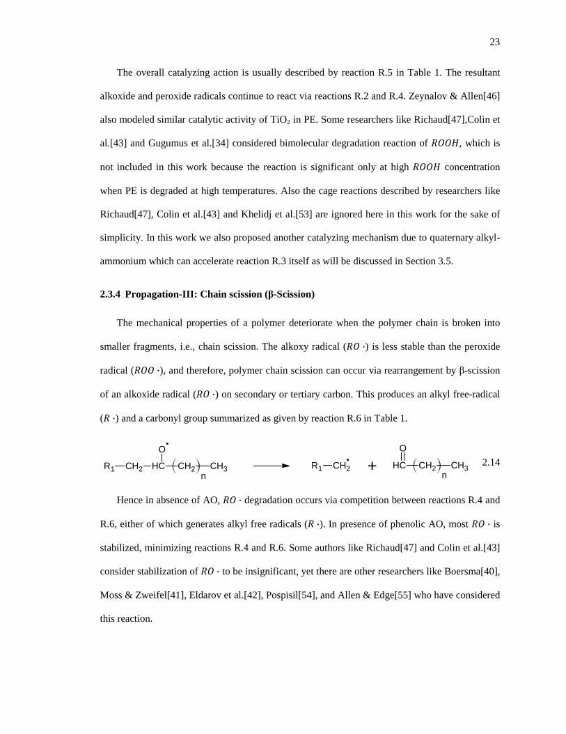
23

The overall catalyzing action is usually described by reaction R.5 in Table 1. The resultant

alkoxide and peroxide radicals continue to react via reactions R.2 and R.4. Zeynalov & Allen[46]

also modeled similar catalytic activity of TiO2 in PE. Some researchers like Richaud[47],Colin et

al.[43] and Gugumus et al.[34] considered bimolecular degradation reaction of ��, which is

not included in this work because the reaction is significant only at high �� concentration

when PE is degraded at high temperatures. Also the cage reactions described by researchers like

Richaud[47], Colin et al.[43] and Khelidj et al.[53] are ignored here in this work for the sake of

simplicity. In this work we also proposed another catalyzing mechanism due to quaternary alkyl-

ammonium which can accelerate reaction R.3 itself as will be discussed in Section 3.5.

2.3.4 Propagation-III: Chain scission (β-Scission)

The mechanical properties of a polymer deteriorate when the polymer chain is broken into

smaller fragments, i.e., chain scission. The alkoxy radical (� ·) is less stable than the peroxide

radical (� ·), and therefore, polymer chain scission can occur via rearrangement by β-scission

of an alkoxide radical (� ·) on secondary or tertiary carbon. This produces an alkyl free-radical

(� ·) and a carbonyl group summarized as given by reaction R.6 in Table 1.

CH2 CH CH2R1 CH3

O

nCH2R1 CH CH2 CH3

O

n+

2.14

Hence in absence of AO, � · degradation occurs via competition between reactions R.4 and

R.6, either of which generates alkyl free radicals (� ·). In presence of phenolic AO, most � · is

stabilized, minimizing reactions R.4 and R.6. Some authors like Richaud[47] and Colin et al.[43]

consider stabilization of � · to be insignificant, yet there are other researchers like Boersma[40],

Moss & Zweifel[41], Eldarov et al.[42], Pospisil[54], and Allen & Edge[55] who have considered

this reaction.

24

2.3.5 Termination-I: Bimolecular combination of free-radi cals

Two free-radicals in close proximity can react with each other giving stable product(s). These

termination reactions decrease the concentration of free radicals responsible for propagation of

the degradation reactions. Therefore, these reactions reduce free radical concentration responsible

further polymer degradation. With three types of free radicals (� ·, � · & � ·), six different

combinations are possible. Some of these types of termination reactions by combination that are

significant in this work are given by reactions R.7 – R.9 in Table 1. Although these reactions have

high rate constants (k� ~ 106 cm3/mol-1s-1[56], k� ~ 1011 cm3/mol-1s-1[57]), the free radical

concentrations in “AO protected” Phase-I are much lower than the alkyl groups in PE or

phenolic/phenoxyl groups in AO. Therefore, Propagation-I, Stabilization and Termination-II

reactions are preferred over these Termination-I reactions throughout Phase-I. As time

progresses, the concentration of phenolic/phenoxyl groups eventually approaches zero and the

‘PE degradation’ Phase-II reactions commence. With no phenolic/phenoxyl groups in Phase-II,

the polymeric free radical concentration increases and termination-I reactions become significant.

Among these polymeric free-radicals, � · is least reactive which can, therefore, accumulate

making reactions R.7 – R.9 potentially significant. Many researchers in the past have considered

only reaction R.7 in their model either in absence of AO [49, 58, 59] or sometimes in presence of

AO [20, 40, 48]. Some other researchers [41, 43, 47] modeled reaction R.7 together with R.8 in

PE degradation. The different types of stable products that might result from these terminations is

not critical in this work because the focus here is more on AO depletion behavior. Hence, a

typical set of products are shown in Table 1.

2.3.6 Stabilization of free-radicals with phenolic AO

An effective way to inhibit PE degradation by free radicals (especially � · & � · because

� · oxidizes as soon as it forms) is to stabilize them with phenolic AOs. The rate constants of AO

stabilization reactions are of the order of 106 cm3/mol-1s-1[51] which is significantly greater than

25

the rate constants of free radicals reacting with alkyl groups in PE that are of the order of 10-3 –

103 cm3/mol-1s-1 (estimated from [60]). Also, the concentration of �� is usually much higher

than free radicals, where �� refers to the active phenolic group on AO. Therefore, as long as

�� is available, stabilization with AO dominates over propagation-I & III, hence averting

polymer degradation. This ��-rich period corresponds to the Phase-I. The higher the

concentration of initial ��, the longer the PE is protected in Phase-I, subject to limits such as

the solubility of �� in the PE matrix.

The main stabilization reactions involving AOs are shown by reactions R.10, R.11 and R.12

in Table 1, where, �� represents a phenolic group on an antioxidant molecule, and � · represents a phenoxyl group than has donated an electron in the process of stabilizing a free

radical.

CH2 CH CH2R CH3

OO

n+ CH2 CH CH2R1 CH3

OOH

nAOH + AO�

2.15

CH2 CH CH2R1 CH3

O

nCH2 CH CH2R1 CH3

OH

n+ AOH + AO�

2.16

+ AOH + AO�CH2 CHR

CH2 CH2

CH3 CH2 CH2R

CH2 CH2

CH3

2.17

In the past works while many researchers [41, 46, 49, 61] considered only stabilization of

peroxide radicals (R.10), some other researchers also considered R.11[40] and R.12[47]together

with reaction R.10.

26

OH

O

O4

(Irganox-1010)

(a)

OH

O

O

(Irganox-1076)

(b)

Figure 2.1. Chemical Structure of the phenolic antioxidants (a) Irganox-1010, and (b) Irganox-1076.

Figure 2.1 shows the molecular structures of two phenolic antioxidants discussed in this

work. Irganox-1010 is a molecule (Figure 1(a)) with four phenolic groups. Each phenolic group

acts as an electron donor (H-transfer) to terminate propagation reactions of the peroxide and

oxide radicals. Therefore each Irganox-1010 molecule is capable of stabilizing four radicals. In

this work ���� is used to represent the concentration of phenolic groups. So each Irganox-1010

molecule contributes four ��. Irganox-1076 (Figure 2.1(b)) is a mononuclear phenol which has

a linear chain hydrocarbon molecule with a phenolic head and is capable of stabilizing only one

free-radical. So each Irganox-1076 molecule contributes only one ��. It has also been reported

that in some cases one phenolic group can stabilize two free-radicals[54] by considering

Termination-II reactions discussed in next section 2.7.

In reactions R.10 and R.11 in Table 1 one phenolic group (��) on an AO molecule

stabilizes one free radical (� · & � ·). Each of these termination reactions can be achieved by

an unreacted phenolic group from either Irganox-1010 or Irganox-1076. Irganox-1076 has been

found to have a higher reactivity than Irganox-1010[62, 63] and both of their reaction constants

are expected to be of the order of 107 cm3/mol-s at 85°C[51].

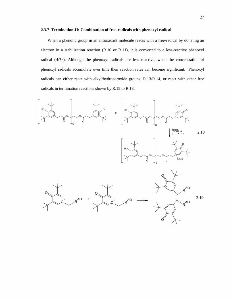
27

2.3.7 Termination-II: Combination of free-radicals with p henoxyl radical

When a phenolic group in an antioxidant molecule reacts with a free-radical by donating an

electron in a stabilization reaction (R.10 or R.11), it is converted to a less-reactive phenoxyl

radical (� ·). Although the phenoxyl radicals are less reactive, when the concentration of

phenoxyl radicals accumulate over time their reaction rates can become significant. Phenoxyl

radicals can either react with alkyl/hydroperoxide groups, R.13/R.14, or react with other free

radicals in termination reactions shown by R.15 to R.18.

OH

O

O

O

O

O3

OH

O

O

C

O

O

O3

OH

O

O

O

O

OOOR

3

+ ROO�

(or RO�/R� )

2.18

C

O

RAO +

C

O

RAO

O

RAO

O

RAO

2.19

28

C

O

RAO +

O

RAO

OR

AO

O

RAO

2.20

The rate constants for the termination reactions R.15 – R.17 can be as high as 109 cm3/mol-s.

These termination reactions reduce the concentration of free radical species available. As will be

shown later in the thesis, these termination reactions are critical for predicting a plateau in ��

concentration towards the end of Phase-I. While the reaction R.16 between phenoxyl radical and

peroxide radical has been modeled by many researchers[41, 42, 46, 47, 61], some works in the

past also considered termination reactions R.18 [46, 47] and R.15 [47] and propagation reaction

R.13 [42, 61].

Oxidation of � · and �� have been considered by authors like Eldarov et al.[42] and

Gugumus[49] but are insignificant under the conditions of this work and, therefore, ignored.

2.4 Summary of reaction assumptions and their rate constants

Under certain conditions, a number of the degradation reactions in Table 1 may be negligible.

As this study is focused on the reactions leading to AO depletion during accelerated thermal

aging (i.e., ‘Phase-I’), some reactions are not incorporated in the model according to the

following assumptions:

• Reaction R.i requires high temperature (>200°C), therefore under the aging conditions

(85°C) it is insignificant and is not included in model.

• Reaction R.0 is significant in nanocomposites when clay acts as catalyst, and is therefore

included in the model.

29

• Reactions R.2 and R.4 are much slower than R.10 and R.11 whenever there is a

significant concentration of AO during ‘Phase-I’; so, alkoxide and peroxide free radical

concentrations are expected to be small. In nanocomposites, there can be higher rates of

generation of these free radicals increasing their concentrations. With higher concentrations

reactions R.2 and R.4 are potentially more significant and are included in the model to explore

their effect in the nanocomposites.

• Reactions R.3 and R.5 have similar functions. R.5 takes place in nanocomposites where

the transition metal ions in clay act as catalyst. The model includes only reaction R.3 as will be

discussed in Chapter 3, Section 3.6.3. Similar to R.5, R.3 might also be enhanced by some other

catalytic mechanism in nanocomposite and will be discussed in section 3.5.

• The chain termination reactions R.7, R.8 and R.9 are negligible as long as phenolic and

phenoxyl groups are present (during Phase-I). During ‘Phase-II’ degradation, concentration of

� · can increase making reaction R.7 significant. Therefore only R.7 is included in the model.

• Reaction R.12 is insignificant in presence of oxygen and is, therefore, not included in the

model.

• Reaction R.14 which is reverse of reaction R.10, is significant only when the

concentration of phenoxyl radical (� ·) is high. This reaction is included in the model because

�� ·� can be high in the nanocomposites.

The important reactions for neat PE and PE-clay nanocomposites are summarized in the

reaction networks of Chapter 3, Figure 3.1. In neat PE the alkyl free radicals are oxidized to

peroxide radicals which are stabilized by AO. These reactions generate hydroperoxide.

Hydroperoxides decompose slowly via R.3 at low temperatures, so generation of new free

radicals is also slow. However, in case of the PE-clay nanocomposites, the model considers fast

hydroperoxide decomposition that generates alkyl and alkoxide radicals and water. The alkoxide

radical is stabilized by AO, and the alkyl radical continues the cycle of its oxidation, AO

30

stabilization, and generation of hydroperoxide. This perpetual R.1- R.10 - R.3 reaction cycle

continuously deprotonates two phenolic groups in AO per cycle. In the nanocomposites this cycle

runs at a faster pace due to increased rate of R.3 leading to faster depletion of AO.

2.5 Reaction parameters

Table 2.2 shows the rate constants of the degradation reactions considered in the model that

are estimated from literature. These values are estimated from reaction rates of smaller molecular

hydrocarbons in liquid phase (like k�, kM), or from experimental data(like k�, k , k��), or predicted

by models of previous researchers (like k�, k��). While estimating reaction rates based on liquid

phase reactions, it was arbitrarily considered that in solid PE the rate would be about 1000 times

slower. The rate constant for stabilization of � ·, k11 is considered to be of similar order as k10.

The rate constant k13 is supposed to be lower than k2. Therefore, in the model the value of k13 is

adjusted to 0.025 cm�/mol. s in order to predict experimental results. In case of PE-clay

nanocomposites, k3 and k5 are the fitting parameters. No fitting parameters are necessary for neat

PE, but k�� requires adjustment within the range of reported values.

Table 2.2. Values of rate constants and other properties in PE as reported in the literature.

Parameters Values Temp. (°C) References

k� 0.57 � 10V� cm�/mol. s 89 [51] Handbook of Polym. Deg., page

394 (2000)

k� 10W cm� mol · s⁄ 85 [51] Handbook of Polym. Deg. (2000)

10�� cm�/mol. s 110 [64] Verdu (2008) (Prediction)

31

Table 2.2 (continued). Values of rate constants and other properties in PE as reported in the literature.

Parameters Values Temp. (°C) References

k

3.4 � 10V cm�/mol. s 27 [51] Handbook of Polym. Deg., page

386 (2000)

7.7 cm�/mol. s 80 [65] Emanuel (1987)

1.7 � 10� cm�/mol. s 110 [64] Verdu (2008) (Prediction)

1.2 � 10 cm�/mol. s 115 [51] Handbook of Polym. Deg., page

385 (2000)

k�� 5 � 10V� sV� 92

[51] Handbook of Polym. Deg., page 395 (2000)

6.6 � 10V� sV� 110 [64] Verdu (2008) (Prediction)

kM 6 � 10V cm�/mol. s -3 [56] Handbook of AOs (1999)

k� ~ 1 s-1 115 [56] Handbook of AOs (1999)

k�

~ 106 cm3/mol-s --- [56] Handbook of AOs (1999)

8.2 �103 cm3/mol-s 30 [51] Handbook of Polym. Deg., page

387 (2000)

5 cm3/mol-s 91 [51] Handbook of Polym. Deg., page

387 (2000)

k�� (Irganox-1010) 12.2 � 10� cm�/mol. s 80 [51] Handbook of Polym. Deg. (2000)

k�M ~ 102 cm3/mol-1s-1 --- [56] Handbook of AOs (1999)

k�� ~ 109 cm3/mol-1s-1 --- [56] Handbook of AOs (1999)

k�� ~ 103 cm3/mol-1s-1 --- [56] Handbook of AOs (1999)

The system of units used by the authors has been converted to standard units

2.6 Physical parameters determining mobility of various species within the polymeric samples

Table 2.3 shows various reported values from literature for diffusivity, solubility and other

related properties that are required for developing and interpreting the lumped parameter and

diffusion-reaction models. Diffusivity of oxygen was found to be reduced by 4-5% in PE-clay

32

nanocomposites. Diffusivity of Irganox-1010 in PE at 85°C can be 1000 times lower than

diffusivity oxygen. Diffusivity of Irganox-1076 is about 10 times higher than Irganox-1010 which

might be attributed to its lower molecular size. Solubilities of oxygen and Irganox-1010 in PE are

on the same order of magnitude when calculated as molar concentrations, while solubility of

Irganox-1076 is about 100 times more. So, a much higher amount of Irganox-1076 can be

introduced in PE but it can also diffuse more quickly to the surface and evaporate. The melting

point and vapor pressure of each AO in Table 2.3 indicate their physical state at sample surface

under experimental conditions and their evaporation rate respectively. Diffusion coefficients of

various polymeric free radical species are also reported that show that they are immobile

compared to the mobility of oxygen and AO.

Table 2.3. Values of various physical properties in PE as reported in the literature

Parameters Values Temp. References

Oxygen diffusivity

4.5 � 10V� cm /s 25°C [51] Handbook of Polym. Deg.,

page 392 (2000)

1.1 � 10V� cm /s 55°C [51] Handbook of Polym. Deg.,

page 392 (2000)

2.0 � 10V� cm /s 55°C [51] Handbook of Polym. Deg.,

page 392 (2000)

2.4 � 10V� cm /s 67°C [51] Handbook of Polym. Deg.,

page 392 (2000)

Oxygen diffusivity in PE with 2% Clay

5.3% reduced 23°C [66] Arunvisut et. al. (2007)

3.8% reduced 20°C [67] Jacquelot et. al. (2006)

Oxygen solubility 1.46 � 10V� mol cm�⁄ 85°C [51] Handbook of Polym. Deg.

(2000)

Irganox-1010 diffusivity

5 � 10V� cm /s 23°C [63] Polymer Additive Analytics

(2006)

2.3 � 10VW cm /s 70°C [63] Polymer Additive Analytics

(2006)

1.2 � 10V� cm /s 85°C [68] Moisan (1980)

33

Table 2.3. (continued) Values of various physical properties in PE as reported in the literature

Parameters Values Temp. References

Irganox-1076 diffusivity

1.5 � 10V�� cm /s 23°C [63] Polymer Additive Analytics

(2006)

4.0 � 10V� cm /s 70°C [63] Polymer Additive Analytics

(2006)

]11 to 23^ � 10V� cm /s 85°C [68] Moisan (1980)

Irganox-1010 Solubility

1.58 � 10V� mol/cm� 60°C [69] Billingham (1981)

1.66 � 10V� mol cm�⁄ 85°C [19] Wong (2012), Estimated

2.53 � 10V� mol/cm� 85°C [68] Moisan (1980)

]3.40 J 4.03^ � 10V� mol/cm� 90°C [63] Polymer Additive Analytics

(2006)

Irganox-1076 Solubility

]25.4 J 35.1^ � 10V� mol/cm� 45°C [63] Polymer Additive Analytics

(2006)

]40.36J 166.01^ � 10V� mol/cm� 85°C [68] Moisan (1980)

Irganox-1010 Vapor Pressure 7.1 � 10V�� mm Hg 25°C

[70] US Environ. Protec. Agency (2001)

Irganox-1076 Vapor Pressure 4.2 � 10V�� mm Hg 25°C

[71] US Environ. Protec. Agency (2001)

Irganox-1010 Melting Temp. 110°C J 125°C N/A

BASF Irganox®1010 MSDS (2010)

Irganox-1076 Melting Temp. 50°C J 55°C N/A

Ciba Irganox®1076 MSDS (1998)

Irganox-1010 Molecular Wt.

1178 N/A BASF Irganox®1010 MSDS

(2010)

Irganox-1076 Molecular Wt.

531 N/A Ciba Irganox®1076 MSDS

(1998)

34

Table 2.3. (continued) Values of various physical properties in PE as reported in the literature

Parameters Values Temp. References

Irganox-1010 Specific Gr.

1.15 N/A BASF Irganox®1010 MSDS

(2010)

Irganox-1076 Specific Gr.

1.02 N/A www.specialchem.com

� · diffusivity 2 � 10V�� cm /s 90°C [56] Handbook of AOs (1999)

� · diffusivity ]10 J 90^ � 10V�� cm /s 90°C [56] Handbook of AOs (1999)

The system of units used by the authors has been converted to standard units

2.7 Conclusions

In the reaction scheme chosen for this work, almost all important reactions leading to AO

depletion during “AO protected” Phase-I are considered with careful exception of those that are

insignificant. Reactions to predict end products of PE degradation are not considered because

they are important only in “PE degradation” Phase-II when all AO is depleted. Therefore with 14

selected reactions in this model, there are 14 rate constant parameters. Most of the work in the

past has used either fewer reactions or an empirical approach to avoid so many parameters. But in

this work, the parameters for PE were found or estimated from existing literature with only a few

such as k16 in neat PE that requires adjustment. In PE-clay nanocomposites, due to catalytic

activity of the clay, values of k0, k’3 and k5 has to be fitted in the model and will be discussed in

the next chapter. This is the first kinetic and diffusion model to predict AO depletion in PE-clay

nanocomposite giving deeper insight to degradation reaction kinetics.

35

CHAPTER 3: REACTION MODEL DESCRIBING ANTIOXIDANT DEPLETION IN SAMPLE CORE

3.1 Introduction

Mathematical modeling and computer simulation of polymer degradation can predict and

give a deep insight into underlying mechanisms in matters of minutes/hours, the experiments for

which would require several years. To simulate the distribution of degradation products,

predicting the evolution of concentrations of all reactant and product species resulting from

significant reactions becomes necessary. But predicting thermal stability of a polymeric material

in terms of antioxidant depletion (referred to as “Phase-I” or the “depletion phase” in this thesis)

does not require the complete set of reactions nor to all possible degradation products.

Antioxidant depletion can be predicted by modeling only those reactions and species that

significantly affect its depletion. The model presented in this chapter does not exactly represent

an accelerated/natural aging, but approximates reality as much as possible. Therefore, the models

serve as a basis for discussion.

The oxidative degradation aging of polymers is being studied since the middle of nineteenth

century when it was found that natural rubber quickly lost its mechanical properties because of

oxidation. Mathematical models of degradation and stability of polymers was developed as early

as 1950 by Tobolsky [31] but received little attention by the researchers causing its slow

development until 1980s. Currently several models exist in the literature accounting for various

kinetic reaction schemes under homogeneous and heterogeneous conditions. The model in this

chapter considers a homogeneous macroscopic scale to predict the antioxidant depletion caused

by thermo-oxidative degradation of PE-clay nanocomposites.

Our prior experimental study of AO depletion in neat PE and nanocomposites[19] has guided

development of the core model presented in this chapter. Here ‘neat PE’ refers to PE with 2wt%

maleic-anhydride grafted PE (MA-g-PE). The core model is a lumped-parameter reaction model

36

to predict core-AO depletion that ignores any additional loss of AO at sample edges.

Consumption of AO in neat PE and its nanocomposite under normal atmospheric conditions may

take several decades; therefore, accelerated thermal aging was used in the experimental study.

Samples were held at 85°C in a circulated air atmosphere, and AO concentrations in aged

samples were determined by measuring ‘oxidation induction times’ (OIT). Although OIT is an

indirect measure of active AO concentration present in a polymeric sample, OIT and AO

concentration are linearly proportional for Irganox-1010 and Irganox-1076 [23-25]. Although

there might exist some deviation from this linear relationship for aged PE and PE-clay

nanocomposites as discussed by Richaud[26] it can still be considered to be linear in all samples

for simplicity. The results showed that in the PE-clay nanocomposite samples, AO depleted at a

much faster rate than neat PE. This could be due to higher rate of decomposition of

hydroperoxides in presence of clay leading to formation of more free radicals[17, 72].

Depletion of AO in PE and PE degradation has been modeled by several researchers. Smith et

al.[73] created a diffusion-reaction model to describe depletion of AO in MDPE pipe incubated in

hot-water at 80°C, 95°C and 105°C. They considered an overall zero order reaction parameter

which depended on AO concentration and position with a diffusion coefficient that varied linearly

with position. Zero order kinetics was chosen because AO depletion was linear for short time

data, but the long-time data invalidates this assumption. The core model predicts an initial linear

decrease in AO concentration without zero order assumption followed by asymptotic approach to

zero to predict long term data. Smith et al. also considered variation in the AO diffusion

coefficient with position to predict the skewedness in AO profiles due to water exposure in inner

side of the pipe and air exposure in the outer side. But this skewedness of the AO profile was not

found in water/water or air/air exposures. A non-uniform initial AO distribution was also used in

the model. Although the justifications for these assumptions were not well developed, the model

agreed with the AO depletion behaviors in PE pipes. Richaud et al.[74] also modeled AO

37

depletion in PE at high temperatures. Their study focused on sulfide AO which stabilizes

hydroperoxides from further decomposition. Unlike Smith, they used chemical reaction schemes

together with physical loss of AO by diffusion of AO into the environment to describe

experimental results. They found that simple kinetic models, where physical loss is either

independent of or proportional to AO concentration, fail to predict experimental results of

concentration versus time at 110°C and 120°C. Therefore, they proposed a new model which

considers an excess AO relative to its saturation threshold in the polymer, which provides a

reservoir for PE stabilization. This modification produced good agreement between the model

and experimental results.

Recently, Gutiérrez et al.[20] studied the influence of clay on oxidation kinetics of

unstabilized PP-clay nanocomposites at temperatures of 60°C, 80°C and 100°C. They measured a

40% reduction in oxygen permeability due to clay addition. Diffusion limitations of O2 caused

carbonyl groups to concentrate in a degraded superficial layer close to the sample surface. The

depth of this layer was 17 µm for PP and 10 µm for the nanocomposites aged at 100°C; this

difference was attributed to decrease in O2 diffusivity by adding clay. The mathematical model

they proposed matched experimental features when the O2 diffusivity in nanocomposites was

40% less than PP. Their study, based on onset of carbonyl group, also shows the induction period

of nanocomposites to be about 30% less than PP. In IR spectroscopy of thermally aged

unstabilized polymers, it is typically observed that carbonyl groups start to appear only after an

initial induction period. This induction period is often used as a measure of stability of a

polymeric material against oxidation. The model considered a cyclic hydroperoxide

decomposition route for generation of newer free radicals. β-scissions of alkoxide radicals were

considered to be instantaneous. To effectively agree with the experimental carbonyl buildup data,

the initial hydroperoxide concentration in the nanocomposite was considered to be twice that of

PP. In unstabilized polymers, the rate of oxygen consumption by free radicals is much higher

38

than in polymers containing antioxidants. Our models (in Chapter 4) have shown that in thin

samples (a few millimeters) of neat PE stabilized with AO, oxygen consumption is slow enough

compared to diffusion that the oxygen quickly saturates and becomes uniform throughout the

sample.

Although there is some prior work in the literature on modeling AO diffusion and depletion

in PE & PP, there are not any published models of AO depletion in PE-clay nanocomposites. This

thesis presents the first model of AO depletion in PE that includes both AO and the effects of

nano-clay. The next section describes the development of mathematical model to predict

concentration of AO and other polymeric reactive groups at different aging times. Diffusion and

physical loss of AO and other reactive species are ignored, so that concentrations of all species

depend on chemical reactions only; the effect of diffusion of both AO and oxygen will be treated

in Chapter 4. The results section discusses a Base-Case result obtained by the model to

understand different features of the model. This is followed by comparison of experimental

results with model predictions to explain the key mechanisms of AO depletion. Some of the key

parameters in the model were adjusted to agree with experimental OIT profiles.

The core model does not consider diffusion of O2 and AO, which can significantly affect the

distribution of different species throughout the depth of the samples. Chapter 4 will present a

model of AO depletion that includes both reactions and diffusion mass transfer. The core model

does not consider any physical interaction of AO with clay such as adsorption onto clay surface.

Therefore, this model serves the purpose of understanding the contribution of chemical reactions

on AO depletion. A homogeneous degradation process is assumed with global concentrations of

AO and other reactive species, which gives average values of PE oxidation behavior. It is known

that phenolic AOs and O2 diffuse only into amorphous phase of PE, therefore, the oxidative

degradation reactions and stabilization takes place in amorphous phase only. However the

assumption of global concentration for all species is justified because the phenolic results are

39

relatively insensitive to the phenolic concentration (shown in section 3.8.2). Different polymeric

reactive species are categorized under alkyl radicals, alkyl groups, oxide and peroxide radicals,

and, hydroperoxides. The reaction rate constants for each of these categorized species are

assumed to have a fixed value at 85°C.

3.2 Model Equations and Assumptions

The rate of oxidative degradation of polymer samples depends on oxygen concentration, the

rates of free radical propagation reactions, and the rate of stabilization of free radicals by reaction

with AO. The mathematical model in the sample core predicts global AO concentration at

different thermal aging times and global concentration for other reacting species as well. In

accelerated aging experiments, all the reactive species are assumed to be immobile and uniformly

distributed throughout the depth of the samples. All reactions are assumed to be first order in each

reactant.

3.2.1 Oxygen Concentration

All reactions in Table 2.1 are assumed to be homogeneous, where kb is the effective reaction

rate constant for reaction R.i and the subscript i represents the respective reaction number. The

oxygen concentration is assumed to be at its saturation level, �O �cde. Oxygen enters the sample

through the surfaces and diffuses rapidly to distribute uniformly. It is assumed that the O2

consumed by reactions R.0 and R.1 is replenished rapidly by absorption of the O2 from the

surrounding atmosphere maintaining its concentration close to its saturation at all times. During

‘Phase-I’ this assumption is valid as generation of � · is limited in the presence of �� and

generation of � · from oxidation of �� (R.0) is negligible. Experimental values of O2 solubility

in PE at different temperatures are available in literature and a typical value of 1.46×10-6 mol/cm3

is reported in Table 2.1.

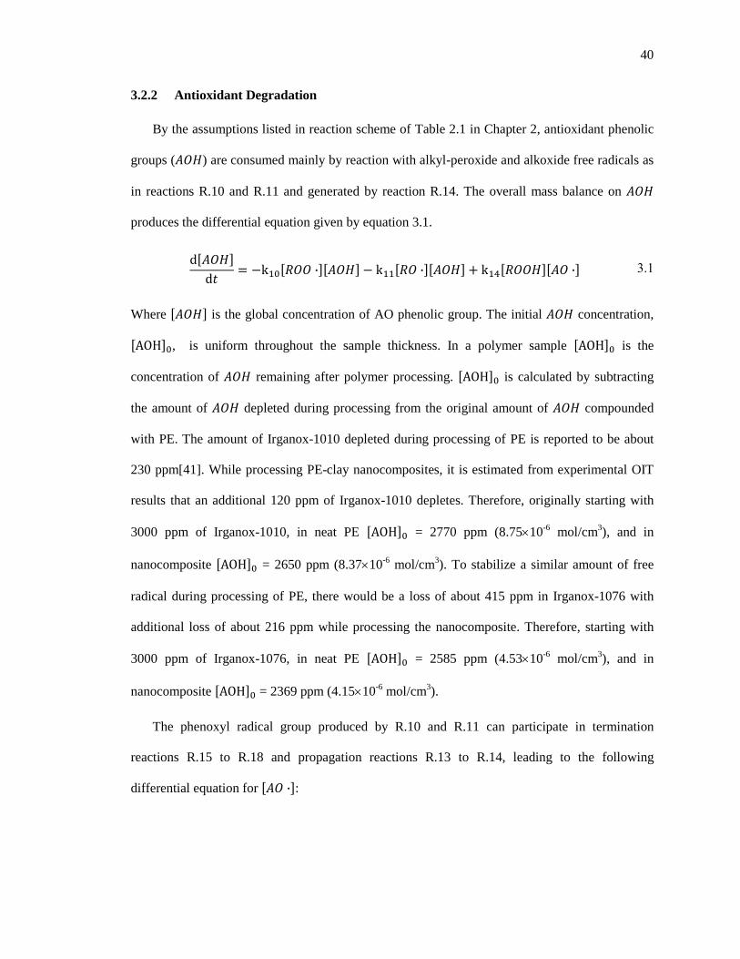
40

3.2.2 Antioxidant Degradation

By the assumptions listed in reaction scheme of Table 2.1 in Chapter 2, antioxidant phenolic

groups (��) are consumed mainly by reaction with alkyl-peroxide and alkoxide free radicals as

in reactions R.10 and R.11 and generated by reaction R.14. The overall mass balance on ��

produces the differential equation given by equation 3.1.

d����df g Jk���� ·����� J k���� ·����� - k�M������ ·� 3.1

Where ���� is the global concentration of AO phenolic group. The initial �� concentration,

�AOH��, is uniform throughout the sample thickness. In a polymer sample �AOH�� is the

concentration of �� remaining after polymer processing. �AOH�� is calculated by subtracting

the amount of �� depleted during processing from the original amount of �� compounded

with PE. The amount of Irganox-1010 depleted during processing of PE is reported to be about

230 ppm[41]. While processing PE-clay nanocomposites, it is estimated from experimental OIT

results that an additional 120 ppm of Irganox-1010 depletes. Therefore, originally starting with

3000 ppm of Irganox-1010, in neat PE �AOH�� = 2770 ppm (8.75×10-6 mol/cm3), and in

nanocomposite �AOH�� = 2650 ppm (8.37×10-6 mol/cm3). To stabilize a similar amount of free

radical during processing of PE, there would be a loss of about 415 ppm in Irganox-1076 with

additional loss of about 216 ppm while processing the nanocomposite. Therefore, starting with

3000 ppm of Irganox-1076, in neat PE �AOH�� = 2585 ppm (4.53×10-6 mol/cm3), and in

nanocomposite �AOH�� = 2369 ppm (4.15×10-6 mol/cm3).

The phenoxyl radical group produced by R.10 and R.11 can participate in termination

reactions R.15 to R.18 and propagation reactions R.13 to R.14, leading to the following

differential equation for �� ·�:

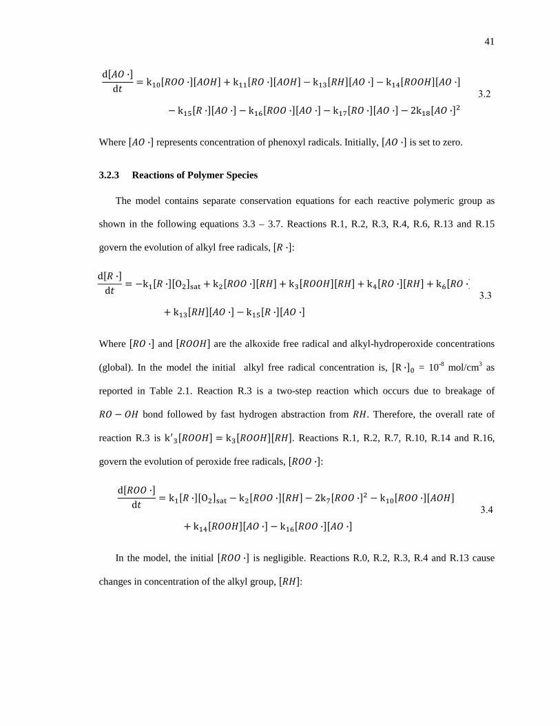
41

d�� ·�df g k���� ·����� - k���� ·����� J k�������� ·� J k�M������ ·�

J k���� ·��� ·� J k���� ·��� ·� J k���� ·��� ·� J 2k���� ·�

3.2

Where �� ·� represents concentration of phenoxyl radicals. Initially, �� ·� is set to zero.

3.2.3 Reactions of Polymer Species

The model contains separate conservation equations for each reactive polymeric group as

shown in the following equations 3.3 – 3.7. Reactions R.1, R.2, R.3, R.4, R.6, R.13 and R.15

govern the evolution of alkyl free radicals, �� ·�: d�� ·�

df g Jk��� ·��O �cde - k �� ·����� - k��������� - kM�� ·����� - k��� ·�- k�������� ·� J k���� ·��� ·�

3.3

Where �� ·� and ���� are the alkoxide free radical and alkyl-hydroperoxide concentrations

(global). In the model the initial alkyl free radical concentration is, �R ·�� = 10-8 mol/cm3 as

reported in Table 2.1. Reaction R.3 is a two-step reaction which occurs due to breakage of

� J � bond followed by fast hydrogen abstraction from ��. Therefore, the overall rate of

reaction R.3 is k������ g k���������. Reactions R.1, R.2, R.7, R.10, R.14 and R.16,

govern the evolution of peroxide free radicals, �� ·�: d�� ·�

df g k��� ·��O �cde J k �� ·����� J 2k��� ·� J k���� ·�����- k�M������ ·� J k���� ·��� ·�

3.4

In the model, the initial �� ·� is negligible. Reactions R.0, R.2, R.3, R.4 and R.13 cause

changes in concentration of the alkyl group, ����:

42

d����df g Jk�������O �cde J k �� ·����� J k������ J kM�� ·�����

J k�������� ·� 3.5

���� is the concentration of sites in PE from where free radicals can abstract hydrogen. The

estimation of initial ���� is described in the next section 3.3. The rate constant of reaction R.0,

k�� is the product of k� reported in Table 2.2 and fraction of �� that accounts for tertiary C-

atoms (i.e., k�� = 0.066 ×k�). It is assumed that this fraction (~0.066) is constant throughout

Phase-I. Reactions R.0, R.2, R.3, R.10 and R.14, cause changes in concentration of

hydroperoxides, ����: d����

df g k�������O �cde - k �� ·����� J k������ - k���� ·�����J k�������� ·�

3.6

In the model, the initial ���� is considered negligible. Reactions R.3, R.4, R.6, R.11 and

R.17, cause changes in concentration of alkoxide radicals, �� ·�:

d�� ·�df g k������ J kM�� ·����� J k��� ·� J k���� ·�����

J k���� ·��� ·� 3.7

Only the polymeric groups � · and �� have significant initial concentrations in the model; all

other polymeric reactive groups are assumed to have zero concentration initially. The ordinary

differential equations (ODEs) in the model were solved numerically using the initial conditions.

The set of ODEs were solved simultaneously using a stiff ODE solver in MATLAB.

3.3 Determination of initial concentration of alkyl groups �i&�j

���� is the concentration of sites in PE from which free radicals can abstract hydrogen. A

highly reactive peroxide/alkoxide radical can abstract hydrogen from almost any C creating a free

43

radical that can later transfer to other C atoms. The most favorable sites for stable free radicals are

those with lowest dissociation energies of the C – H bond in the order of: allyl > tertiary >

secondary > primary. The degree of unsaturation in PE can vary between 0 – 4 per 1000 C atoms

[75]. As allyl-carbon can be present on either side of a C=C double bond in PE molecule,

therefore, there can be 0 – 8 allyl-carbons per 1000 C to donate hydrogen to free radicals. Also,

β-scission of alkoxide radicals, and various rearrangement of free radicals can result in

unsaturation throughout the PE degradation process [76]. Concentration of tertiary C can be

estimated from branch density of PE. A recent study shows branch density in pure PE of about 2

per 1000 C[77]. Additionally, each maleic anhydride molecule (present at 1wt% of compatibilizer

MA-g-PE) contributes one tertiary carbon. Therefore 0.02wt% maleic anhydride in PE samples

contributes 0.02 – 0.04 branches per 1000 C atoms. Abstraction of hydrogen from secondary and

primary C requires higher activation energy than allylic and tertiary C. With no allyl or tertiary

carbon in close proximity of a free radical, it can abstract hydrogen from a secondary or even

from a primary carbon. As the concentration of secondary C is much more than any other type of

C, some authors like Richaud et al.[26] calculated ����� by finding molar concentration of

methyl groups. However, the free radical generated on secondary/primary C can undergo

intra/inter molecular transfer to less reactive tertiary/allylic C. This hypothesis is supported by the

study of Gryn’ova et al.[78] where they found H abstraction by peroxide radical from secondary

C of many polymers including PE to be strongly thermodynamically unfavorable, because the

bond dissociation energy of the corresponding C–H bond is significantly higher, than that of the

ROO–H bond. Accordingly H abstraction only becomes thermodynamically favorable when the

product radical is stabilized by allylic double bonds. Therefore, the tertiary/allylic carbon sites are

preferred over primary/secondary C for donating hydrogen to free radicals, and hence are

considered reactive centers in PE molecule. There can be over 10 such sites in 1000 C atoms (i.e.,

over 2 sites per 100 ethyl monomer repeat units). In the model, it is assumed to have 10 such sites

per 1000 C according to the following breakdown:

44

• Allylic C–H ~ 4 in 1000 carbon

• Tertiary C–H ~ 2 in 1000 C

• Others (other allylic C–H formed during processing, etc.) ~ 4 in 1000 C

It has been assumed that the free radicals generated due to hydrogen abstracted from

primary/secondary C are transferred to allylic/tertiary C which are at higher concentration than

free radicals generated during Phase-I. An analysis described in Appendix B shows that hydrogen

abstraction from secondary C can be 25 times slower than hydrogen abstraction from allylic C,

and 4 times slower than hydrogen abstraction from tertiary C. Therefore, primary/secondary C are

not counted as effective reactive sites. Each �� (alkyl group) is assumed to consist of one

reactive site. Therefore, with 10 reactive sites in 1000 C, each �� consists of about 100 C or 50

ethyl monomer repeat units. This gives an estimation of concentration of the alkyl group to be on

the order of 10-4 mol/cm3. This is much higher than free radical species which are on the order of

10-8 mol/cm3. The high concentration of alkyl groups together with its slow decay makes ���� fairly constant over the period of AO depletion.

3.4 Cyclic reactions during Phase-I

The concentrations of the reactive polymer groups mainly depend on the dynamic cycles of

free radical reactions shown in Figure 3.1 for both neat PE (Figure 3.1(a)) and PE

nanocomposites (Figure 3.1(b)). In this work, “neat PE” refers to polyethylene containing

compatiblizers but which does not include any nano-particles. The primary cycle in both neat PE

and nanocomposites is oxidation of alkyl radicals via R.1, stabilization of peroxide radicals via

R.10, and decomposition of hydroperoxides via R.3 to regenerate alkyl radicals. Values of

various reaction rate constants reported in the literature are discussed in Chapter 2, and Table 3.1

contains values that have been chosen for the core reaction model. In Figure 3.1, all of the

arrows, text for chemical formulas, and circles for reaction rate constants are sized to indicate

their relative magnitude, but the size is not to scale because some values vary by many orders of

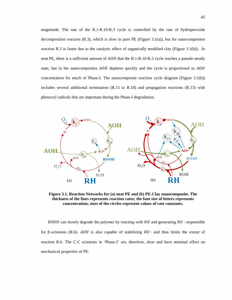
45

magnitude. The rate of the R.1-R.10-R.3 cycle is controlled by the rate of hydroperoxide

decomposition reaction (R.3), which is slow in pure PE (Figure 3.1(a)), but for nanocomposites

reaction R.3 is faster due to the catalytic effect of organically modified clay (Figure 3.1(b)). In

neat PE, there is a sufficient amount of �� that the R.1-R.10-R.3 cycle reaches a pseudo steady

state, but in the nanocomposites �� depletes quickly and the cycle is proportional to ��

concentration for much of Phase-I. The nanocomposite reaction cycle diagram (Figure 3.1(b))

includes several additional termination (R.15 to R.18) and propagation reactions (R.13) with

phenoxyl radicals that are important during the Phase-I degradation.

Figure 3.1. Reaction Networks for (a) neat PE and (b) PE-Clay nanocomposite. The thickness of the lines represents reaction rates; the font size of letters represents

concentration; sizes of the circles represent values of rate constants.

�� can slowly degrade the polymer by reacting with �� and generating � · responsible

for β-scissions (R.6). �� is also capable of stabilizing � · and thus limits the extent of

reaction R.6. The C-C scissions in ‘Phase-I’ are, therefore, slow and have minimal effect on

mechanical properties of PE.

ROOH

ROO•

R•

H2O

O2

AOH

ROH

AO•

AOH

RH

k16

k

18

k17

k11

k

3

RO•

k13

(a) (b)

k1

k

10

ROOH

ROO•

R•

H2O

O2

AOH

ROH

AO•

AOH

RH

k

18

k11

k3

RO•

k1

k

10

46

Neat PE samples are modeled using parameters found in the literature which are listed in

Table 3.1. The rate constant k�� was varied to account for differences in reactivity of the two

antioxidants, Irganox-1010 and Irganox-1076. For predictions of nanocomposites, only the rate

constant k��, was adjusted to achieve qualitative agreement between model predictions and

experimentally-measured OIT profiles.

3.5 Justification of a high hydroperoxide decomposition rate constant k�l in nanocomposites

In addition to reaction equations R.3 and R.5 there are other potential mechanisms for

hydroperoxide decomposition such as the catalytic effect of ammonium ion present inside

modified clay-galleries that is exposed to PE molecules especially when the clay layers exfoliate

Equations 3.8 – 3.11 present a mechanism similar to one proposed by Napadensky and

Sasson[79].

�� - ]�^�mn]"opq^V *++++, � r � r ]�^�mn]"opq^V 3.8

� r � r ]�^�mn]"opq^V *++++, � · - ]�^�mn�V - ]"opq^ · 3.9

� · - ]"opq^ · *++++, � g - �n]"opq^V 3.10

]�^�mn�V - �n]"opq^V *++++, ]�^�mn]"opq^V - � 3.11

Here, ]�^�mn is the quaternary-alkyl ammonium ion, ]"opq^V is an anion on clay, and ]"opq^ · is a free radical on clay. The � · generated in this mechanism is expected to be much more

reactive than ]"opq^ ·. Therefore, in addition to the reaction given in equation 3.10, it can also

participate in other reactions like R.4, R.6, R.11 and R.17. Also, if the free radical on clay,

]"opq^ ·, instead of terminating with � · (via equation 10) reacts with ��, then an alkyl free

radical, � ·, can be generated as given by equation 3.12.

]"opq^ · - �� *++++, �n]"opq^V - � · 3.12

47

Therefore, the overall reaction for this catalytic hydroperoxide decomposition is similar to

reaction R.3. The value of rate constant of reaction R.3 (k��) required to match the experimental

slope of �� depletion in PE-clay nanocomposites is ~103 times larger than the values reported

in literature for neat PE which is justified by this mechanism.

3.6 Results & Discussions

3.6.1 Model Predictions for a base case ‘Comp.1010’

The reaction model predicts depletion of AO, and concentration of polymeric reactive groups

as a function of time. Typical results for a base case are shown in Figure 3.2 and Figure 3.3.

Parameters used for these results are the same as for PE-Clay nanocomposites with Irganox-1010,

which are listed in Table 3.1 under the column Comp.1010. Table 3.1 also mentions the relative

significance of each of these parameters in depleting AO as predicted by the model.

Predictions of �� depletion for the Base Case are shown in Figure 3.2(a) and (b), and the

concentrations for reactive polymeric groups are shown in Figure 3.3. �� concentration is

normalized by the initial phenolic group concentration. � · and other reactive groups are scaled

with initial � · group concentration. The scaled concentrations of most of the polymeric reactive

groups vary between zero and one as appears in Figure 3.3. The ratio of initial concentration of

�� (in Irganox-1010) to initial concentration of � · is �AOH�� �R ·��⁄ = 837. Therefore, the

initial �� concentration is much higher than concentration of any of the free radical species. So

depletion of �� requires formation of new free radical groups during the oven aging at 85°C as

depicted by the cycles in Figure 3.2.

48

Figure 3.2. (a) Depletion of phenolic group concentration, �$%&�, as predicted by the model for typical accelerated aging conditions of PE-Clay nanocomposites. (b) Same plot in

logarithmic time scale. The insets are magnification of certain sections and error in model-fitting comparison. The parameters used for this figure correspond to ‘Base Case’ of

Comp.1010 in Table 3.1. Experimental data is included for comparison.

The ���� depletion versus time curve in Figure 3 exhibits several periods: (1) a short

initiation period of less than 40 days, (2) a linear depletion period until 65 (±1% error) days, (3)

an asymptotic depletion period until about 1300 days, and (4) a depleted period corresponding to

101

102

103

0

0.1

0.2

0.3

0.4

0.5

0.6

0.7

0.8

0.9

1

101

102

103

0

0.1

0.2

0.3

0.4

0.5

0.6

0.7

0.8

0.9

1

Time, days

[AO

H]/[

AO

H]

0

103

0

0.02

0.04

0.06

Time, days

[AO

H]/[

AO

H]

0

101

102

103

-0.01

-0.005

0

0.005

0.01

Time, days

Diff

ere

nce

b/w

Mo

del a

nd

Line

ar

& E

xpo

nent

al F

it

Exponential

Linear

Model Prediction

Exponential

Experimental

Model Predictions

Exponential Fit

Linear Fit

(b)

(a)

0 200 400 600 800 1000 1200 1400 16000

0.2

0.4

0.6

0.8

1

0 200 400 600 800 1000 1200 1400 16000

0.2

0.4

0.6

0.8

1

[AO

H]/[

AO

H]

0

Time, days

Lin

ear

Initi

atio

n

35 40 45 500.84

0.86

0.88

90 100110120

0.65

0.7

Model Predictions

Experimental(Comp.1010)

Exponential Fitting

Linear Fitting

550 600 650 7000.06

0.08

0.1

0.12

0thOrder AO* reactions become more important1st Order

Phase-I

AOH/AO*Depleted

Asymptotic Depleted

Phase-II

49

Phase-II degradation. About 35% of the �� depletes during the linear period due to the R.1-

R.10-R.3 reaction cycle of Figure 3.1(b). In the asymptotic period, the ���� decays to zero and

the termination reactions lead to a reduction in the concentration of hydroperoxides, leading to a

deceleration of the R.1-R.10-R.3 cycle. As ���� and [� ·] tend to zero towards the end of

Phase-I, there are no mechanisms to significantly control the growth of free radicals, and the

Phase-II degradation reactions commence.

Figure 3.3 shows that during Phase-I, the reactive polymer groups � ·, � ·, � ·, and

�� all exhibit a short initial period in which they change rapidly followed by a long period in

which they are nearly constant or slowly varying; however, at the start of Phase-II (~1300 days)

all of these species exhibit rapidly changing concentrations. During the initial period � · instantly

oxidizes to � ·; �� then stabilizes the � · rapidly driving the peroxide free radical

concentration to much less than �� ·� s 10V��R ·��. This stabilization of � · produces �� and � · with concentrations approximately equal to �R ·��. Under the

assumption of saturated oxygen, all these reactions take place in less than a second. �� is also

generated via Reaction R.0 due to the catalytic effect of clay. The �� produced reacts slowly

with PE to form � · and � · radicals via R.3. In addition, the � · reacts with PE, although

slowly, to generate � · via R.13. The regenerated alkyl radical, � · from these reactions reacts

instantaneously with O2 forming � ·, and these � · and � · radicals are again stabilized by

�� in a cyclic fashion causing a decreasing ���� as shown in Figure 3.2. In this reaction

cycle, oxidation of free radicals (R.1) and consecutive regeneration of �� (R.10) are so fast

compared to �� decomposition (R.3) that the free radical concentrations are close to zero and

�� accumulates as shown in Figure 3.3(b). During the initial period (< 40 days),

���� �R ·��⁄ exceeds 1 because reaction R.13 slowly adds more � · into the cycle.

50

Figure 3.3. Concentration of various polymeric reactive groups for typical accelerated aging conditions of PE-Clay nanocomposites ‘Base Case’: (a) alkyl groups i&, (b) hydroperoxides i%%&, (c) phenoxyl radicals $% ·, (d) alkyl radicals i ·, (e) peroxide radicals i%% ·, and, (f) alkoxide radicals i% ·. All concentrations are normalized by the initial alkyl free radical

concentration, �i ·�j. Inset figures display the same data with magnified vertical axis.

The stabilization reactions generate � · radicals which are capable of termination by

coupling with itself or by combination with polymeric free radicals. Although slow, the

termination of � · and � · radicals by combination with � · (R.16 and R.17) can be

significant. This reduces the burden on �� in stabilizing these radicals. � · is generated at

nearly same rate as �� but reacts at slower rate. So their growth and decline patterns follow

similar trend with a lower accumulation of � · around 50 days of aging as shown in Figure 3.3(b

& c). The termination of reactions R.16 and R.17 limits the accumulation of �� ·� and �� ·� which otherwise would continue to increase. This causes the concentrations of the polymeric free

radicals to be nearly constant for most of Phase-I (inner plots of Figure 3.3(e) and 3.3(f)). With

nearly constant �� ·� and �� ·�, the rate of ���� depletion reaction is approximately first

order causing an exponential depletion in ���� as shown by exponential fit in Figure 3.2. The

0 500 1000 15000

0.2

0.4

0.6

0.8

1

Time, days

[R*]

/[R*]

0

0 500 1000 15000

2000

4000

6000

8000

10000

Time, days

[RH

]/[R

*]0

0 500 1000 15000

0.2

0.4

0.6

0.8

1

Time, days

[RO

O*]

/[R*]

0

0 500 1000 15000

2

4

6

8

10

Time, days

[RO

OH

]/[R

*]0

0 500 1000 15000

0.2

0.4

0.6

0.8

1

Time, days

[RO

*]/[R

*]0

0 500 1000 15000

2

4

6

8

10

Time, days

[AO

*]/[R

*]0

0 500 1000 15000

0.2

0.4

0.6

0.8

1

Time, days

[R*]

/[R*]

0

0 500 1000 15000

2000

4000

6000

8000

10000

Time, days

[RH

]/[R

*]0

0 500 1000 15000

0.2

0.4

0.6

0.8

1

Time, days

[RO

O*]

/[R*]

0

0 500 1000 15000

2

4

6

8

10

Time, days

[RO

OH

]/[R

*]0

0 500 1000 15000

0.2

0.4

0.6

0.8

1

Time, days

[RO

*]/[R

*]0

0 500 1000 15000

2

4

6

8

10

Time, days

[AO

*]/[R

*]0

0 500 1000 15000

0.5

1

Time, days

[R*]

/[R*]

0 x

106

0 500 1000 15000

0.5

1

Time, days

[RO

O*]

/[R*]

0 x 1

06

0 500 1000 15000

0.5

1

Time, days

[RO

*]/[R

*]0 x

106

(b) (c)

(d) (e)

(a)

(f)

51

inset of Figure 3.2(b) showing the between error model and fitting shows that the exponential is a

good fit to the full model. In addition, during a short initial period ���� �AOH��⁄ is close to 1

(approximately until 100 days), and, the rate of ���� depletion is nearly constant corresponding

to a linear depletion (as shown by linear fit in Figure 3.2) or zero order kinetic as reported by

Smith et al.[73]. From 100 – 600 days, ���� depletes exponentially transitioning from linear to

asymptotic depletion. Reducing ���� decreases the rates of stabilization reactions and

regeneration of �� causing a continuous decline in ���� during Phase-I as shown in

Figure 3.3(b).

In Figure 3.2, ���� decreases to about 2% of its initial value in 1000 days of aging. This

reduction in ���� in turn reduces stabilization rate of � · causing �� ·� to accumulate as

shown in the inner plot of Figure 3.3(e) after about 1000 days. Reactions R.10, R.11, R.16 and

R.17 limit the accumulation of polymeric free radicals until about 1300 days after which ���� and �� ·� becomes nearly zero. Beyond this period there are no �� or � · to inhibit the

growth of free radicals and the Phase-II degradation reactions commence.

Phase-II starts with a sudden increase in free radical concentrations as appears in Figure 3.3

at about 1300 days. During this time, one � · oxidizes (R.1) to � · which reacts with �� (R.2)

to regenerate one � · and one ��. The �� then reacts with �� (R.3) to generate another

� · and � ·. � · then undergoes β-scission (R.6) generating yet another � ·. Therefore, one � · can regenerate three free radicals in one cycle, each of which can again oxidize and propagate the

cyclic reactions. When the oxidation accelerates in Phase-II, the assumption of constant O2

concentration might not be valid, and O2 supply can become diffusion limited as will be discussed

in next chapter. Among these reactions R.2 and R.3 are the slowest causing accumulation of

� · (Figure 3.3(e)) and �� (Figure 3.3(b)). With increasing �� ·�, its termination by

coupling (R.7) becomes significant. Concentrations of � · and � · are close to zero because

reaction R.1 and R.6 are fast. Reactions R.2 and R.3 degrades �� and results in addition of

52

carbonyl and hydroxyl groups to PE molecules. C-C β-scission via reaction R.6 is responsible for

the degradation of mechanical properties of PE. Further details of all these Phase-II degradation

reactions are beyond the scope of this thesis.

Table 3.1. Parameters used in the model to predict AO depletion in neat PE and its clay nanocomposites. The parameters in bold font are most important parameters. For the right three columns, ‘---’ corresponds to the same parameters as in the Base Case. The values in

italics were adjusted to achieve good agreement between model and experiments.

Parameters Significance

(determined by changing one parameter at a time)

Comp.1010 (Base Case)

Values different than Base Case

NeatPE1010 NeatPE1076 Comp.1076

k'0 ucm3 mol·s⁄ v Insignificant for k�� s 10V� 10-8 --- --- ---

k1 ucm3 mol·s⁄ v Slows AO depletion if

k� s 10W 109 --- --- ---

k2 ucm3 mol·s⁄ v No asymptote of AO if k w 10�

1 --- --- ---

kkkk ''''3333 xssss‐‐‐‐1111y Negligible AO depletion for k�� s 10V�, Not rate limiting

for k�� w 10VM, 1.0 ×10-5 10-8 10-8 ---

k4 ucm3 mol·s⁄ v AO depletes rapidly when kM w 10�

10 --- --- ---

kkkk6666 ussss‐‐‐‐1111v AO depletes rapidly when k� w 1 1 --- --- ---

k7 ucm3 mol·s⁄ v Slows AO depletion when k� w 10�M

1010 --- --- ---

kkkk10101010 ucmcmcmcm3333 mol·smol·smol·smol·s⁄ v AO depletion slow for k�� s10� and fast for k�� w 10�

107 --- --- ---

kkkk11111111 ucmcmcmcm3333 mol·smol·smol·smol·s⁄ v AO depletes rapidly when k�� s 10�

107 --- --- ---

kkkk13131313 ucmcmcmcm3333 mol·smol·smol·smol·s⁄ v AO depletion slow for k�� s0.027 and fast for k�� w 0.027

0.027 --- --- ---

k14 ucm3 mol·s⁄ v Slows AO depletion when k�M w 10

102 --- --- ---

kkkk15151515 ucmcmcmcm3333 mol·smol·smol·smol·s⁄ v Slows AO depletion when k�� w 10W

109 --- --- ---

kkkk16161616 ucmcmcmcm3333 mol·smol·smol·smol·s⁄ v

AO depletion slow for k�� w9×10� and fast for k�� s9×10� 9×108 --- 7×109 7×109

k17 ucm3 mol·s⁄ v Slows duration of asymptotic

AO depletion when k�� w 10�� 109 --- --- ---

53

Table 3.1. (continued) Parameters used in the model to predict AO depletion in neat PE and its clay nanocomposites. The parameters in bold font are most important

parameters. For the right three columns, ‘---’ corresponds to the same parameters as in the Base Case. The values in italics were adjusted to achieve good agreement between

model and experiments.

Parameters Significance

(determined by changing one parameter at a time)

Comp.1010 (Base Case)

Values different than Base Case

NeatPE1010 NeatPE1010 NeatPE101

0

kkkk18181818 ucmcmcmcm3333 mol·smol·smol·smol·s⁄ v AO depletion slow for k�� s10� and fast for k�� w 10�

103 --- --- ---

�RHRHRHRH�0000 umolmolmolmol cmcmcmcm3333⁄ v

AO depletion slow for �RH�� s10VM and fast for �RH�� w10VM 10-4 --- --- ---

�R·�0 umol cm3⁄ v Significant initial AO deletion

for �R ·�� w 10V� 10-8 --- --- ---

�AOHAOHAOHAOH�0000 umolmolmolmol cmcmcmcm3333⁄ v

AO depletion slow for �AOH�� s 10V� and fast for �AOH�� w 10V� 8.37×10-6 8.75×10-6 4.53×10-6 4.15×10-6

�OOOO2222�satsatsatsat umolmolmolmol cmcmcmcm3333⁄ v AO depletion slow for �O �cde, s 10V�

10-6 --- --- ---

3.6.2 Estimation of k�l from initial linear AO Depletion in the R.1-R.10-R.3 Reaction Cycle.

After a short initiation period, the ���� depletion predicted by the model is approximately

linear until about 100 days. This section provides a simplified analysis to estimate k�� in

nanocomposites from experimental slope of initial linear �� depletion. �� depletion in neat

PE follows the R.1-R.10-R.3 reaction cycle of Figure 3.1(b). In this cycle of reactions, ��

decomposition is the rate controlling step for PE because the other reactions are relatively fast.

This results in accumulation of �� until its concentration is roughly equal to the initial � · concentration. The ���� concentration actually rises to more than �� ·�� because � · propagation slowly supplies additional � · via reaction R.13 and tertiary carbon oxidation

supplies additional �� via reaction R.0. When �� decomposes by R.3, it is quickly

54

replenished by R.1 and R.10 maintaining a high ���� concentration as long as ���� is

sufficiently high (above ~ 65% of �AOH��) to maintain the cycle. Because ���� and ���� are

approximately constant after the initial transient (Figure 4(b) & Figure 4(a)) until about 65 days

(within ±1% error), the rate of reaction (R.3) is approximately constant during that period, which

is denoted as C� in equation 3.13 below.

k��������� g C� = (1.5 ±0.3) ×10-13 mol/cm3-s 3.13

Here the estimate of C� is calculated from the known value of ���� z ����� and assuming that

���� equals the initial � · concentration (10-8 mol/cm3). Ignoring reactions R.0, R.2 and R.16,

the rate of change of ���� (~10-16 mol/cm3-s) given by equation 3.14 is small relative to "�.

k���� ·����� J C� g d����df { C� 3.14

Neglecting the rate of change of ���� and various slow/insignificant reactions (R.4, R.6,

R.7, R.14, R.17), and, assuming that the concentration of polymeric reactive groups �� ·�, and

�� ·� are in pseudo steady state, the concentration of different free radicals groups can be

estimated from equations 3.4, 3.7 and 3.3 as follows:

�� ·�/�R ·�� g C� k�������R ·��⁄ ≈ 2.7 ×10-7 3.15

�� ·�/�R ·�� g C� k�������R ·��⁄ ≈ 2.7 ×10-7 3.16

�� ·�/�R ·�� g C� k��O �|de�R ·��⁄ ≈ 1.5 ×10-8 3.17

These predictions are in qualitative agreement with the solution of the ODEs in the model as

shown in the insert figures of Figure 3.3(d), 3.3(e) & 3.3(f) between 40 to 100 days. Furthermore,

when the estimated concentrations are plugged in equation 3.1, the rate of depletion of ���� is

found to be constant and equal to 2· C�. This relationship was used to estimate the reaction rate

55

constant k� from experimental data as follows where �ROOH�}|| and �RH�}|| are concentrations

in the pseudo-steady-state period.

k� = – slope/2�ROOH�}||�RH�}|| ≈ – slope/2�R ·���RH�� 3.18

The parameter k� for the Base Case predictions is estimated from the initial

experimental slope of Comp.1010 of about 1.72×10-8 mol/cm3-days, which when plugged in

equation 3.18, gives the value of k� to be 0.10 cm3/mol-s. Therefore, k�� g k����� zk��RH�� = 1.0 ×10-5 cm3/mol-s as appears in Table 3.1.

3.6.3 Analysis of Alternatives for Hydroperoxide Decomposition

In presence of transition metal in clay acting as catalyst, hydroperoxides can decompose via

the bimolecular hydroperoxide decomposition reaction R.5 as described by equations 2.12 and

2.13 in Chapter 2. This mechanism of hydroperoxide decomposition is very fast, and therefore

has been identified by other authors as the cause of severe �� depletion in the nanocomposites

[17]. However, the analysis in this section shows that this reaction does not lead to the

experimentally observed �� depletion and that �� decomposition by R.3 provides better

predictions of experimental data.

If R.5 were the controlling mechanism for hydroperoxide decomposition, then the reaction

cycle would be R.1-R.10-R.5 (rather than R.1-R.10-R.3 of Figure 3.1(b)). The key difference

between these cycles is that two hydroperoxides molecules react in R.5 whereas only one

hydroperoxide molecule reacts in R.3. The two free radical products of R.5 (� · and � ·) are

both stabilized by ��, but only stabilization of � · creates a hydroperoxide; stabilization of

� · via R.11 produces an alcohol �� which does not react further. Consequently in the R.1-

R.10-R.5 cycle the concentration of hydroperoxide is continuously decreasing. Detailed analysis

is provided in the section 3.8.1, but if the R.1-R.10-R.5 cycle were the only cycle leading to

depletion of ��, then the total amount of �� depleted would be on the order of 3�R ·�� which

56

is less than 1% of the initial concentration of ��. Therefore bimolecular decomposition of

hydroperoxides via R.5 cannot be the dominant mechanism for severe �� depletion.

Another mechanism by which clay could affect �� concentration is reaction of oxygen

with tertiary-C on PE molecules (��) generating hydroperoxides (��) as given by reaction

R.0. Figure 3.4 displays predictions in which this reaction is enhanced by 104 with reaction

constant k�� at a value of about 10-8 s-1. This reaction can be catalyzed by transition metal ions

present in clay as given by equations 2.5 – 2.6 in Chapter 2. As concentration of tertiary-C is

assumed to be proportional to ��, and �� is fairly constant in Phase-I, rate of reaction R.0 is

also a constant. (R.0 would decelerate if tertiary-C were to deplete.) With continuous generation

of �� and its slow decomposition (via R.3), ���� would increase continuously during

Phase-I and the rate of reaction R.3 would also increase with time. Contrary to experimental

observations, the rate of �� depletion in Figure 3.4 accelerates for the first 600 days. This

mechanism also does not predict experimentally observed depletion of ��. Therefore, among

the two catalytic �� decomposition mechanisms (R.3 and R.5) and one catalytic generation

mechanism of ��, R.3 as described in Section 3.5 is the only mechanism that provides good

predictions of experimental �� depletion while using reasonable rate constants.

Figure 3.4. Prediction for $%& concentration with reaction R.0 enhanced by 104. The rest of the parameters used for this figure correspond to ‘NeatPE1010’ in Table 3.1.

0 200 400 600 800 1000 1200 1400 16000

0.2

0.4

0.6

0.8

1

Time, days

[AO

H]/[

AO

H]

0

Model PredictionsExperimental(Comp.1010)

0 200 400 600 800 1000 1200 1400 16000

0.2

0.4

0.6

0.8

1

Time, days

[AO

H]/[

AO

H]

0

57

3.6.4 Significance of various bimolecular free-radical terminations during later times of Phase-I

Parametric studies with the model (discussed later) have shown that bimolecular termination

reactions are necessary for predicting the exponential decay and asymptotic period of ��

depletion. Table 3.2 lists all possible bimolecular free radical combination reactions for polymeric

free radicals and phenoxyl free radicals. The rates of free radical termination by combination of

reactions R.7, R.8 and R.9 are very slow. Although their reaction rate constants can be very high

in PE at 85°C (k� ∼109 cm3/mol-s[53]), the concentrations of � ·, � · and � · are on the order

of 10-15 mol/cm3 or less rendering the reaction rates to be very slow. As discussed in 3.6.1, the

concentrations of these groups are low because �� stabilizes them via reaction R.10 and R.11

as soon as they are generated. �� stabilizes free radicals and generates phenoxyl radicals (� ·) that are less reactive than polymeric free radicals. But the concentration of phenoxyl radical can

be 107 times higher than other radicals, and hence termination reactions via phenoxyl radicals

(R.15, R.16, R.17) is significant even though its termination rate constants are low.

Table 3.3 displays rough estimates of the rates of termination reactions. The rate constants for

termination involving polymeric radicals are expected to be around 109-1010 cm3/mol-s, and for

coupling of phenoxyl radical with another phenoxyl radical the rate constant is expected to

around 103 cm3/mol-s[56, 80]. These rate constants were included in the model, and used to

predicted the concentrations of various radical species as appears in first column of Table 3.3 (at

around 400 days). The reaction rates for each termination reaction were then calculated as

displayed in Table 3.3. The termination reactions involving phenoxyl radicals are ten orders of

magnitude or faster than the other termination reactions. Among the termination reactions

involving phenoxyl radicals (R.15 – R.18), reactions R.16 and R.18 are critical in determining the

shape of �� depletion, as observed in a parametric study (discussed in section 3.8.5). Although

reactions R.15 and R.17 are also significant, their influence in determining the shape of ��

58

depletion is insignificant or less significant at values of reaction constants (k�� & k��) considered

in Table 3.1.

Table 3.2 Bimolecular termination reactions by combination of free radicals.

Eq.# R.No Termination-I & III Reactions

--- R.7 � · -� · (E *++, R=O - O - ROH

Combination of peroxide radicals

--- R.7a � · -� · (E~ *+++, 2�� Coupling of alkyl free radicals

--- R.7b � · -� · (E� *+++, �� Coupling of alkoxide radicals

--- R.8 � · -� · (F *++, �� Termination of alkyl radical

by peroxide radical

--- R.9 � · -� · (G *++, ROR - O2

Termination of alkoxide radical by peroxide radical

(proposed)

--- R.9a � · -� · (G~ *+++, ROR Termination of alkyl radical

by alkoxide radical

2.18 R.15 � · -� · (>C *+++, AO]R^ Termination of alkyl radical

by phenoxyl radical

2.18 R.16 � · -� · (>D *+++, AO]ROO^ Termination of peroxide

radical by phenoxyl radical

2.18 R.17 � · -� · (>E *+++, AO]RO^ Termination of oxide radical

by phenoxyl radical 2.18, 2.19

R.18 � · -� · (>F *+++, AO]AO^ Coupling of phenoxyl radicals

Other researchers have also considered these termination reactions to be important[56, 61].

Reactions R.16 and R.17 interrupt the cyclic reactions of Figure 3.1(b) by limiting the growth of

� · and � ·. This maintains a nearly constant �� ·� and �� ·� which promotes the ��

depletion to follow first order kinetics. Hence, there is a gradual shift of �� depletion from

linear to flat as shown in Figure 3.2.

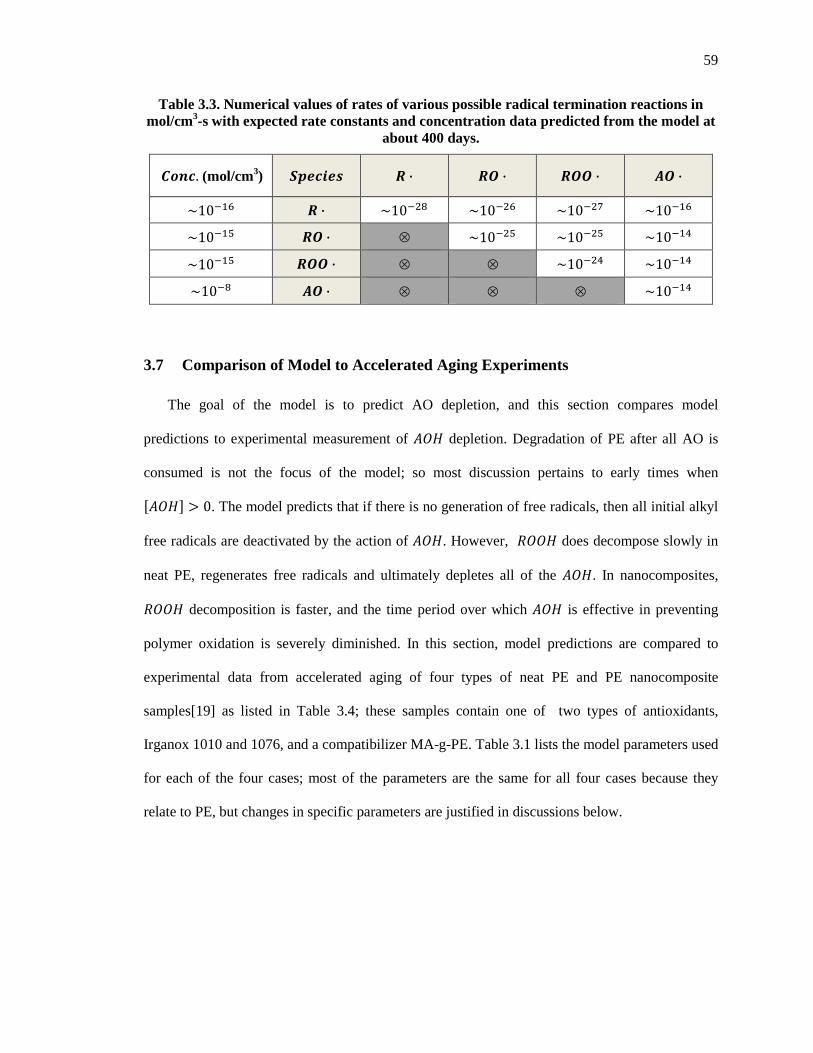
59

Table 3.3. Numerical values of rates of various possible radical termination reactions in mol/cm3-s with expected rate constants and concentration data predicted from the model at

about 400 days.

����. (mol/cm3) ������� i · i% · i%% · $% · ~10V�� i · ~10V � ~10V � ~10V � ~10V��

~10V�� i% · ⊗ ~10V � ~10V � ~10V�M

~10V�� i%% · ⊗ ⊗ ~10V M ~10V�M

~10V� $% · ⊗ ⊗ ⊗ ~10V�M

3.7 Comparison of Model to Accelerated Aging Experiments

The goal of the model is to predict AO depletion, and this section compares model

predictions to experimental measurement of �� depletion. Degradation of PE after all AO is

consumed is not the focus of the model; so most discussion pertains to early times when

���� w 0. The model predicts that if there is no generation of free radicals, then all initial alkyl

free radicals are deactivated by the action of ��. However, �� does decompose slowly in

neat PE, regenerates free radicals and ultimately depletes all of the ��. In nanocomposites,

�� decomposition is faster, and the time period over which �� is effective in preventing

polymer oxidation is severely diminished. In this section, model predictions are compared to

experimental data from accelerated aging of four types of neat PE and PE nanocomposite

samples[19] as listed in Table 3.4; these samples contain one of two types of antioxidants,

Irganox 1010 and 1076, and a compatibilizer MA-g-PE. Table 3.1 lists the model parameters used

for each of the four cases; most of the parameters are the same for all four cases because they

relate to PE, but changes in specific parameters are justified in discussions below.

60

Table 3.4. Samples used in accelerated aging tests.

Sample Name Sample Code

AO (wt%) Clay (wt%)

MA-g-PE* (wt%)

PE (wt%) I-1010 I-1076

NeatPE1010 F-1 0.3 -- 0 2 97.7

Comp.1010 F-2 0.3 -- 4 2 93.7

NeatPE1076 F-3 -- 0.3 0 2 97.7

Comp.1076 F-4 -- 0.3 4 2 93.7

*MA-g-PE contains 1% maleic-anhydride

Figure 3.5. Comparison of experimental results with model predictions for $%&

concentration in NeatPE1010. [19, 81]

0 200 400 600 800 1000 1200 1400 16000

0.2

0.4

0.6

0.8

1

0 200 400 600 800 1000 1200 1400 16000

0.2

0.4

0.6

0.8

1

Time, days

[AO

H]/[

AO

H]

0

Experimental (NeatPE1010)

Model with [AOH]0 = initial experimental

Model with [AOH]0 = 62% of experimental

Experimental (Bulk OIT with 0.1 wt% I-1010)

Model Predictions for 0.1 wt% I-1010

Asymptotes to Model Predict ions with [AOH]0 = 62% of Experiment

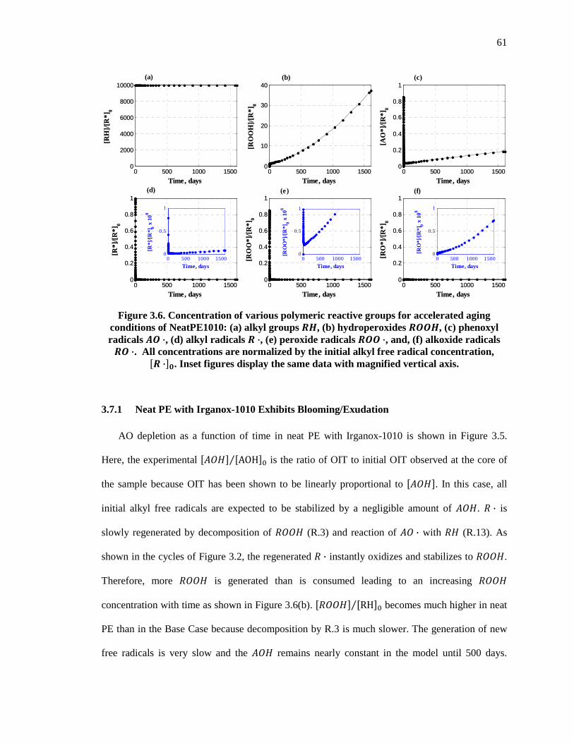
61

Figure 3.6. Concentration of various polymeric reactive groups for accelerated aging

conditions of NeatPE1010: (a) alkyl groups i&, (b) hydroperoxides i%%&, (c) phenoxyl radicals $% ·, (d) alkyl radicals i ·, (e) peroxide radicals i%% ·, and, (f) alkoxide radicals i% ·. All concentrations are normalized by the initial alkyl free radical concentration, �i ·�j. Inset figures display the same data with magnified vertical axis.

3.7.1 Neat PE with Irganox-1010 Exhibits Blooming/Exudation

AO depletion as a function of time in neat PE with Irganox-1010 is shown in Figure 3.5.

Here, the experimental ���� �AOH��⁄ is the ratio of OIT to initial OIT observed at the core of

the sample because OIT has been shown to be linearly proportional to ����. In this case, all

initial alkyl free radicals are expected to be stabilized by a negligible amount of ��. � · is

slowly regenerated by decomposition of �� (R.3) and reaction of � · with �� (R.13). As

shown in the cycles of Figure 3.2, the regenerated � · instantly oxidizes and stabilizes to ��.

Therefore, more �� is generated than is consumed leading to an increasing ��

concentration with time as shown in Figure 3.6(b). ���� �RH��⁄ becomes much higher in neat

PE than in the Base Case because decomposition by R.3 is much slower. The generation of new

free radicals is very slow and the �� remains nearly constant in the model until 500 days.

0 500 1000 15000

0.2

0.4

0.6

0.8

1

Time, days

[R*]

/[R*]

0

0 500 1000 15000

0.2

0.4

0.6

0.8

1

Time, days

[R*]

/[R*]

0

0 500 1000 15000

2000

4000

6000

8000

10000

Time, days

[RH

]/[R

*]0

0 500 1000 15000

2000

4000

6000

8000

10000

Time, days

[RH

]/[R

*]0

0 500 1000 15000

0.2

0.4

0.6

0.8

1

Time, days

[RO

O*]

/[R*]

0

0 500 1000 15000

0.2

0.4

0.6

0.8

1

Time, days

[RO

O*]

/[R*]

0

0 500 1000 15000

10

20

30

40

Time, days

[RO

OH

]/[R

*]0

0 500 1000 15000

10

20

30

40

Time, days

[RO

OH

]/[R

*]0

0 500 1000 15000

0.2

0.4

0.6

0.8

1

Time, days

[RO

*]/[R

*]0

0 500 1000 15000

0.2

0.4

0.6

0.8

1

Time, days

[RO

*]/[R

*]0

0 500 1000 15000

0.2

0.4

0.6

0.8

1

Time, days

[AO

*]/[R

*]0

0 500 1000 15000

0.2

0.4

0.6

0.8

1

Time, days

[AO

*]/[R

*]0

0 500 1000 15000

0.5

1

Time, days

[RO

O*]

/[R*]

0 x 1

08

0 500 1000 15000

0.5

1

Time, days

[RO

*]/[R

*]0 x

108

0 500 1000 15000

0.5

1

Time, days

[R*]

/[R*]

0 x 1

08

(b) (c)(a)

(d) (e) (f)

62

Unexpectedly, the experimental OIT values for NeatPE1010 show a decreasing trend as shown in

Figure 3.5. This decrease has been attributed to blooming of �� to the surface of the

sample[19]. Blooming (also called as exudation) occurs when initial AO content is higher than

the solubility limit, thus the excess AO diffuses to the surface and accumulates as an AO-rich

film on the sample surface, sometimes termed as surface precipitation[63]. Wong and Hsuan[81]

shows that lowering the initial AO concentration by about one-third eliminates this ‘blooming’

phenomenon because in that case �AOH�� is well below the saturation limit (shown by data points

marked with triangles in Figure 3.5). In the experiments with ���� above saturation (open

circles in Figure 6), AO diffuses out of the sample forming a pure AO deposit on the surface until

it reaches its saturated concentration, �AOH�cde, which is about 62% of the originally introduced

amount of AO (corresponding to OIT value of the layer adjacent to surface in aged NeatPE1010

samples which will be discussed in next chapter). Within this reaction model rather than

modeling blooming directly, the initial ���� is assumed to be at 62% of the amount that was

originally added to the sample (green curve in Figure 3.5).

3.7.2 Nanocomposites with Irganox-1010 Exhibits Linear followed by Asymptotic Depletion

�� depletion as a function of time in Comp.1010 under forced-air conditions is shown in

Figure 3.7 for the first 500 days and in the Base Case predictions from Figure 3.2 and Figure 3.3.

Here, experimental ���� �AOH��⁄ is the ratio of measured OIT to initial OIT. The parameters

used in the model are for the Base Case of Comp.1010 as given in Table 3.1 and only differ from

the parameters in for NeatPE1010 in a few ways; the rate constants for R.1 and R.3 are higher due

to the catalytic effect of clay and the initial �� concentration is a slightly lower due to

additional depletion during processing. The experimentally-measured ���� is roughly linear for

the first six data points (up to 262 days). In the model decomposition of �� via reaction R.3

is the mechanism that regenerates � · and drives more rapid depletion of ����. As

63

discussed in section 3.6.1, the model predicts that termination of � · and � · by � · (R.16

and R.17) limits their growth, and �� ·� and �� ·� are constant for much of Phase-I. This

causes ���� to deplete nearly exponentially (approximately first order reaction where the rate

of ���� depletion is proportional to ����). This causes a smooth transition of ���� depletion from linear to asymptotic. � · also generates � · via reaction R.13. When � · is

terminated by � · (R.16), a similar amount of � · is replenished via oxidation of � · produced

by reaction R.13. Therefore, the rate constants of reactions R.13 and R.16 were adjusted to match

with the experimental data.

Figure 3.7. Comparison of experimental results with model predictions for AO concentration in Comp.1010

The core reaction model presented in this chapter is complicated and contains many

parameters. The majority of the parameters were obtained from the literature and the estimated

values of the remaining parameters are justified above. During the process of developing this

model, several simpler models were used that provided reasonable prediction of experimental

data but required unrealistic parameter values. The following subsections provide examples of

simpler models and changes in parameter values required for agreement with experiments with

the Comp.1010.

0 100 200 300 400 5000

0.2

0.4

0.6

0.8

1

Time, days

[AO

H]/[

AO

H]

0

Model PredictionsExperimental(Comp.1010)

0 100 200 300 400 5000

0.2

0.4

0.6

0.8

1

Time, days

[AO

H]/[

AO

H]

0

64

3.7.2.1 Case-I: No phenoxyl-radical reactions

Free radical termination reactions are normally neglected during early stages of degradation.

When the rate constants for all of the phenoxyl-radical reactions (R.13 to R.18) are set to zero and

reactions R.6, R.7 and R.12 are ignored, the �� concentration depletes linearly until it is nearly

completely exhausted at about 370 days as shown by Case-Ia in Figure 3.8. This is because with

reduction in ����, �� ·� and �� ·� accumulate such that the right hand side of equation 3.1

remains constant. �� decomposes to generate an equal amount of � ·, almost all of which

stabilizes to regenerate the original amount of �� (Case-Ia in Figure 3.9(d)).

Once all �� is consumed, � · and � · produced by Reactions R.3 and R.1 are no

longer stabilized. This corresponds to a sudden increase in free radical concentrations as appears

in Figure 3.9 at about 370 days. At this time, accumulation of � · and � · radicals

regenerates � · via reactions R.2 and R.4. � · which oxidize and react with �� in a cyclic

fashion increasing the concentrations of ��, � · and � ·. This cyclic reaction leads to an

uncontrolled rapid degradation of ��.

The model without termination by phenoxyl radicals (� ·) is not able to predict the last two

experimental data points for Comp.1010. A potential resolution is to define a ‘residual AO’ which

is not functional in protecting the polymer or a minimum OIT due to the induction time of the

neat PE itself. This is supported by experimental OIT values that do not always decrease to zero,

but rather asymptote to a ‘residual’ value. The green line in Figure 3.8 corresponds to this case

with a residual �� of 10% of the initial �� concentration and produces acceptable agreement

with experimental data. However, this value of residual �� is large and unreasonable when

compared with values reported in literature[82] where it is reported to be about 2% or less.

65

Figure 3.8. Depletion of AO, predicted by the model without phenoxyl-radical reactions for accelerated aging conditions of Comp.1010. The parameters used for this figure correspond

to different cases in Table 3.5.

Figure 3.9. Concentration of various polymeric reactive groups for the cases of Figure 3.8:

(a) alkyl radicals i ·, (b) peroxide radicals i%% ·, (c) alkoxide radicals i% ·, and, (d) hydroperoxides i%%&. All concentrations are normalized by the initial alkyl free radical concentration, �i ·�j. The parameters used for these predictions are presented in Table 3.5.

0 100 200 300 400 5000

0.1

0.2

0.3

0.4

0.5

0.6

0.7

0.8

0.9

1

0 100 200 300 400 5000

0.1

0.2

0.3

0.4

0.5

0.6

0.7

0.8

0.9

1

Linear Depletion of AOHTime, days

[AO

H]/[

AO

H]

0

Case-Ia (without residual AO)

Case-Ib (with residual AO)

Case-IIa (low k2 & k

9 with residual AO)

Case-IIb (no k2 & low k

9 with residual AO)

Base Case

Experimental

Residual AOH

0 100 200 300 400 5000

0.2

0.4

0.6

0.8

1

0 100 200 300 400 5000

0.2

0.4

0.6

0.8

1

0 100 200 300 400 5000

0.2

0.4

0.6

0.8

1

0 100 200 300 400 5000

0.2

0.4

0.6

0.8

1

0 100 200 300 400 5000

0.2

0.4

0.6

0.8

1

Time, days

[R.]

/[R*]

0

0 100 200 300 400 5000

0.2

0.4

0.6

0.8

1

Time, days

[RO

O.]

/[R*]

0

0 100 200 300 400 5000

0.2

0.4

0.6

0.8

1

Time, days

[RO

OH

]/[R

*]0

0 100 200 300 400 5000

0.2

0.4

0.6

0.8

1

Time, days

[RO

.]/[R

*]0

(a) (b)

(c) (d)

66

Table 3.5. Values of reaction parameters used in the simplified models of Case-I and Case-II without phenoxyl reactions to predict AO depletion in Comp.1010. For the right

three columns, ‘---’ corresponds to the same parameters as in Base Case.

Parameters Base Case

values

Values different than Base Case

Case-Ia in Figure 3.8

Case-Ib in Figure 3.8

Case-IIa in Figure 3.8

Case-IIb in Figure 3.8

k�, ]cm� mol · s⁄ ^ 10V� 0 0 0 0

k�, ]cm� mol · s⁄ ^ 10W --- --- --- ---

k , ]cm� mol · s⁄ ^ 1 --- --- 10V� 0

k��RH�, ]sV�^ 1.0 � 10V� 1.3 � 10V� 1.3 � 10V� 1.3 � 10V� 2.5 � 10V�

kM, ]cm� mol · s⁄ ^ 10 --- --- --- ---

k��, ]cm� mol · s⁄ ^ 10� --- --- 6 6

k��, ]cm� mol · s⁄ ^ 10� --- --- --- ---

Termination Reactions (k�, k�� J k��)

As in Base Case of Table 2 0 0 0 0

� · Propagation Reactions (k�� & k�M)

As in Base Case of Table 2 0 0 0 0

Residual �� 0 0 10% 10% 10%

3.7.2.2 Case-II: Slower stabilization of peroxide radicals with no phenoxyl reaction create smoother transition from linear to asymptotic depletion

The cases shown by ‘Case-Ia’ and ‘Case-Ib’ lines in Figure 3.8 use parameters that are

reported in literature (included in Table 2.2) but has a sharp transition between linear AO

depletion and asymptotic AO depletion. The sharp transition between linear and flat AO depletion

is due to very fast reaction of �� with � · (R.10). If this stabilization reaction is slower, and

the reaction between � · and �� (reaction R.2) is negligible; then the model predicts a smooth

transition of AO depletion from linear to flat as shown by the ‘Case-IIa’ line in Figure 3.8 based

on parameters Case-IIa in Table 3.5. Another way to predict a smooth transition of AO depletion

from linear to flat is by incorporating higher rate of �� decomposition, slower stabilization

reaction (R.10), no reaction R.2 as shown by the ‘Case-IIb’ line in Figure 3.8 based on parameters

Case-IIb in Table 3.5. In both of these cases, the reaction R.10 is the slowest and is therefore rate

67

controlling. The assumption of pseudo steady state on concentrations of � ·, � · and ��

does not hold true in this case as evident by purple and red curves in Figure 3.9. When the

concentration of �� is high, it depletes linearly, but as �� concentration becomes small, it

reduces the rate of AO depletion (reaction R.10) causing a smooth transition to a flat residual AO

concentration. Residual AO in these cases are assumed to be 10% of original AO. In Case-IIb

(red), the transition is even smoother than Case-IIa (purple) in Figure 3.8 because there is no

sudden decrease in ���� due to its faster decomposition rate as appears in Figure 3.9(d).

In Case-IIa the value of k is assumed to be 10-3 cm3/mol-s and in Case-IIb k2 is assumed to

be zero. The actual value of k depends on dissociation energy of C-H bond and is therefore very

selective. For stable bonds like hydrogen belonging to aromatic rings, k ∼10-4 cm3/mol-s at 27°C,

and for unstable bonds like hydrogen belonging to allylic carbon atom, k ∼500 cm3/mol-s at

27°C[80]. Therefore, the low values of k used to predict purple and red lines in Figure 3.8 is

questionable. Also, the value of k�� is considered to be 6 cm3/mol-s in these cases to make

reaction R.10 rate limiting to give smooth transition. This is more than a million times lower than

typical reported values as given in Table 2.2. In these cases, the AO would be ineffective in

protecting the polymer from degradation, and the polymer would degrade via reaction R.2.

The examples of simplifying the model in Figure 3.8 and Figure 3.9 provide reasonable

agreement with experimental data but utilize unrealistic values of the parameters. To achieve

good agreement between the predictions and experimental data while also using reaction

parameters consistent with the literature, it is necessary to include rapid stabilization reactions

and free-radical termination reactions that become significant as phenoxyl radicals accumulate in

the sample.

3.7.3 No Depletion in ‘NeatPE1076’

In NeatPE1076, AO does not significantly deplete over the course of a year at 85°C as shown

in Figure 3.10 for both model predictions and experimental data. Blooming is not observed

68

because the solubility for Irganox-1076 is much higher than the initial Irganox-1076

concentration. Based on the reaction network of Figure 3.1(a), Irganox-1076 does not deplete

because the concentration of free radicals is stabilized by a negligible amount of AO, which is

about 0.2% of its original amount. In neat PE, the hydroperoxide decomposition is much slower

than in nanocomposites; so regeneration of newer free radicals via cycle R.1-R.10-R.3 is slow.

AO depletion due to reaction in both NeatPE1010 and NeatPE1076 are quite similar, and are

modeled using the same reaction network. The values of reaction parameters used are also same

(A higher value of ��� is considered for consistency with Comp.1076 and is not critical because

�� ·� is small in neat PE). Both have negligible AO depletion by reaction. In the experiments,

NeatPE1010 has a greater physical loss of AO compared to NeatPE1076 due to blooming.

Figure 3.10. Comparison of experimental results with model predictions for $%& concentration in NeatPE1076’.

3.7.4 Slow Core Depletion in Comp.1076

AO depletion as a function of time in Comp.1076 is shown in Figure 3.11 based on model

parameters from Table 3.1. Here, experimental ���� �AOH��⁄ is the ratio OIT to maximum OIT

0 100 200 300 400 5000

0.2

0.4

0.6

0.8

1

1.2

Time, days

[AO

H]/[

AO

H]

0

0 100 200 300 400 5000

0.2

0.4

0.6

0.8

1

1.2

Time, days

[AO

H]/[

AO

H]

0

69

value of Comp.1076. Surprisingly, the experimental �� concentration in the sample core

increases during the first 2 months of aging and then starts to decrease. This increase has been

related to adsorption of AO molecules onto nanoclay platelet surfaces and then subsequent

desorption [19]. This initial rise is not predicted by the model, which does not account for AO

adsorption onto clay; rather, the initial �� concentration was adjusted to be the same as the

second data point as a rough approximation. The numerical value of the OIT of the second data

point (20.4 min.) of the Comp.1076 sample is similar to the initial OIT value of the NeatPE1076

sample (22.4 min.) and appears to be a better representation of the amount of �� originally

present in the sample.

Except for the initial increase in AO concentration, the model predictions are qualitatively in

good agreement with experimental observations. In the model, slow �� depletion is achieved

by higher reactivity of phenoxyl radical (� ·) in Irganox-1076 than the phenoxyl radical in

Irganox-1010. This can be attributed to higher mobility of Irganox-1076 than Irganox-1010

together with the different molecular structures; each Irganox 1010 molecule has four phenoxyl

radicals which can reduce their overall reactivity. The higher reactivity of the phenoxyl radical in

Comp.1076, accelerates termination via reaction R.16 and reduces the � · concentration

(Figure 3.12(e)) to ten times less than concentration predicted for Comp.1010 (Figure 3.3(e)) and

slows the stabilization reaction R.10. This causes slower ���� depletion in Comp.1076 than in

Comp.1010. Based on these predictions, Irganox 1076 is a more effective antioxidant for

polyethylene nanocomposites. Utilizing antioxidants that have higher phenoxyl termination rates

likely will create nanocomposites with better durability.

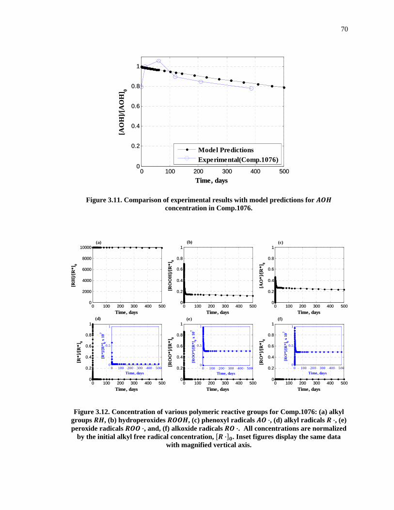
70

Figure 3.11. Comparison of experimental results with model predictions for $%& concentration in Comp.1076.

Figure 3.12. Concentration of various polymeric reactive groups for Comp.1076: (a) alkyl groups i&, (b) hydroperoxides i%%&, (c) phenoxyl radicals $% ·, (d) alkyl radicals i ·, (e) peroxide radicals i%% ·, and, (f) alkoxide radicals i% ·. All concentrations are normalized

by the initial alkyl free radical concentration, �i ·�j. Inset figures display the same data with magnified vertical axis.

0 100 200 300 400 5000

0.2

0.4

0.6

0.8

1

Time, days

[AO

H]/[

AO

H]

0

Model PredictionsExperimental(Comp.1076)

0 100 200 300 400 5000

0.2

0.4

0.6

0.8

1

Time, days

[AO

H]/[

AO

H]

0

0 100 200 300 400 5000

0.2

0.4

0.6

0.8

1

Time, days

[R*]

/[R*]

0

0 100 200 300 400 5000

2000

4000

6000

8000

10000

Time, days

[RH

]/[R

*]0

0 100 200 300 400 5000

0.2

0.4

0.6

0.8

1

Time, days

[RO

O*]

/[R*]

0

0 100 200 300 400 5000

0.2

0.4

0.6

0.8

1

Time, days

[RO

OH

]/[R

*]0

0 100 200 300 400 5000

0.2

0.4

0.6

0.8

1

Time, days

[RO

*]/[R

*]0

0 100 200 300 400 5000

0.2

0.4

0.6

0.8

1

Time, days

[AO

*]/[R

*]0

0 100 200 300 400 5000

0.2

0.4

0.6

0.8

1

Time, days

[R*]

/[R*]

0

0 100 200 300 400 5000

2000

4000

6000

8000

10000

Time, days

[RH

]/[R

*]0

0 100 200 300 400 5000

0.2

0.4

0.6

0.8

1

Time, days

[RO

O*]

/[R*]

0

0 100 200 300 400 5000

0.2

0.4

0.6

0.8

1

Time, days

[RO

OH

]/[R

*]0

0 100 200 300 400 5000

0.2

0.4

0.6

0.8

1

Time, days

[RO

*]/[R

*]0

0 100 200 300 400 5000

0.2

0.4

0.6

0.8

1

Time, days

[AO

*]/[R

*]0

0 100 200 300 400 5000

0.5

1

Time, days

[R*]

/[R*]

0 x 1

07

0 100 200 300 400 5000

0.5

1

Time, days

[RO

O*]

/[R*]

0 x 1

07

0 100 200 300 400 5000

0.5

1

Time, days

[RO

*]/[R

*]0 x

107

(a) (b) (c)

(d) (e) (f)

71

3.8 Additional Analysis

3.8.1 Description of AO Depletion in the R.1-R.10-R.5 Reaction Cycle

If R.5 were the controlling mechanism for hydroperoxide decomposition, then the reaction

cycle would be R.1-R.10-R.5 (rather than R.1-R.10-R.3 of Figure 3.1(b)). The key difference

between these cycles is that two hydroperoxides molecules react in R.5 whereas only one

hydroperoxide molecule reacts in R.3. The two free radical products of R.5 (� · and � ·) are

both stabilized by ��, but only stabilization of � · creates a hydroperoxide; stabilization of

� · via R.11 produces an alcohol �� which does not react further. Consequently in the R.1-

R.10-R.5 cycle the concentration of hydroperoxide is continuously decreasing.

Figure 3.13. Various reactive species in reaction cycle via R.5 in which the concentration of reactive species halve in each cycle to eventually discontinue it.

The R.1-R.10-R.5 cycle is depicted in Figure 3.13 where the widths of the arrows represent

concentration of the reactive species in each cycle. Initially all � · gets converted to �� which

then produces � ·. Concentration of � · produced is half the amount of original ����. In

the next cycle, the concentration of � · reduces to a quarter of original ����. This

reduction of � · continues in a similar fashion in each cycle until it totally runs out of � · to

fuel the cycle. Therefore eventually the cycle comes to an end.

– AO•

– RO•

R1 R10

R5

– H2O

– RO•

R5

– H2O

– AO•

R10

– AO•

R10

[ROOH] reduces by half in each cycle to approach zero

2nd

cycle 3rd cycle 1

st cycle

72

With reaction R.5, and ignoring slow/insignificant reactions, the differential equations 3.4

and 3.6 become:

��� ·��f z ������ J ����� ·����� 3.19

������f z J2������ - ����� ·����� 3.20

It is worthy to note that in this case, there is a net loss of ���� per cycle. This is because

in one reaction cycle, one moles of �� is generated when two moles of �� is

decomposed. Therefore, eventually all �� is decomposed, and the cycle stops before AO

depletion. Therefore, this reaction cycle fails to predict complete AO depletion.

Total �� depleted until the cycle ends can be calculated from mass balance on this reaction

cycle. The cycle starts with alkyl free radicals �� ·��, and when the cycle ends it therefore

produces an equal molar concentration of alkoxide radicals, �� ·�� g �� ·��. Regeneration of

alkyl radicals has to be in the same amount as alkoxide radicals due to reaction R.5 all of which

are oxidized to � · and recycled. Therefore, original �� ·�, recycled �� ·� and generated �� ·� all contribute to depletion of ����. So, the total depletion of ���� is equal to 3�� ·��.

Therefore, for complete AO depletion by the R.5 cycle the amount of �� ·�� required is at least

one-third of �����. For parameters used in “Base Case”, this much �� ·�� corresponds to 3×10-

6 mol/cm3 for complete AO depletion. When compared with experimental data reported in

literature (see Table 2.2), this appears to be 100-1000 times more and therefore is questionable.

Also, it is interesting to note that one-third of total �� depletion takes place in the first

cycle. Therefore under such situation, the initial OIT would reflect ���� that is two-thirds of

�����. As this cycle does not exist in neat PE, so the initial OIT of it should reflect �����. So,

the initial OIT of nanocomposite (Base Case) would be two-third of OIT of neat PE. In case of

Irganox-1010 this does not hold true as will be evident in the next section. Therefore, it is

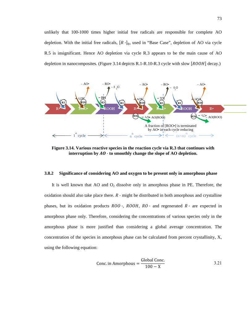
73

unlikely that 100-1000 times higher initial free radicals are responsible for complete AO

depletion. With the initial free radicals, �� ·��, used in “Base Case”, depletion of AO via cycle

R.5 is insignificant. Hence AO depletion via cycle R.3 appears to be the main cause of AO

depletion in nanocomposites. (Figure 3.14 depicts R.1-R.10-R.3 cycle with slow ���� decay.)

Figure 3.14. Various reactive species in the reaction cycle via R.3 that continues with interruption by $% · to smoothly change the slope of AO depletion.

3.8.2 Significance of considering AO and oxygen to be present only in amorphous phase

It is well known that AO and O2 dissolve only in amorphous phase in PE. Therefore, the

oxidation should also take place there. � · might be distributed in both amorphous and crystalline

phases, but its oxidation products � ·, ��, � · and regenerated � · are expected in

amorphous phase only. Therefore, considering the concentrations of various species only in the

amorphous phase is more justified than considering a global average concentration. The

concentration of the species in amorphous phase can be calculated from percent crystallinity, X,

using the following equation:

Conc. in Amorphous g Global Conc.100 J X 3.21

– AO(ROO) R16

– AO•

– RO•

R1 R10 R3

– H2O

– AO•

– RO•

R1 R10 R3

– H2O

– AO•

R1 R10

A fraction of [ROO•] is terminated by AO• in each cycle reducing

[ROOH]

– AO(ROO) R16

nth cycle (n+m)

th cycle 1

st cycle

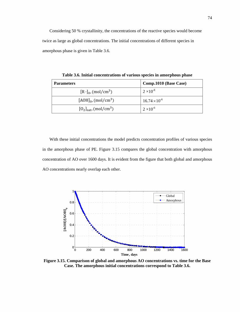
74

Considering 50 % crystallinity, the concentrations of the reactive species would become

twice as large as global concentrations. The initial concentrations of different species in

amorphous phase is given in Table 3.6.

Table 3.6. Initial concentrations of various species in amorphous phase

Parameters Comp.1010 (Base Case)

�R ·��, ]mol cm�⁄ ^ 2 ×10-8

�AOH��, ]mol cm�⁄ ^ 16.74 ×10-6

�O �cde, ]mol cm�⁄ ^ 2 ×10-6

With these initial concentrations the model predicts concentration profiles of various species

in the amorphous phase of PE. Figure 3.15 compares the global concentration with amorphous

concentration of AO over 1600 days. It is evident from the figure that both global and amorphous

AO concentrations nearly overlap each other.

Figure 3.15. Comparison of global and amorphous AO concentrations vs. time for the Base

Case. The amorphous initial concentrations correspond to Table 3.6.

0 200 400 600 800 1000 1200 1400 16000

0.2

0.4

0.6

0.8

1

0 200 400 600 800 1000 1200 1400 16000

0.2

0.4

0.6

0.8

1

Time, days

[AO

H]/[

AO

H]

0

GlobalAmorphous

75

It might be argued that initially alkyl free radicals are distributed in both amorphous and

crystalline phases. If this is true then �R ·�� in Table 3.6 would be same as global �R ·�� (i.e. 10-8

mol/cm3). With this assumption, the comparison of global and amorphous AO depletion is shown

in Figure 3.16. Here also, there is not much difference in AO depletion behavior.

Hence, it is concluded that considering amorphous concentrations instead of global

concentrations is not critical. As long as crystallinity does not vary during the degradation

process, it is therefore acceptable to develop a model using overall (global) concentration.

Figure 3.16. Comparison of global and amorphous AO concentrations vs. time for the Base

Case. This is different than Figure 3.15 because here initial i · concentration is same for both global & amorphous cases.

Considering amorphous concentration might become important if results/predictions are

compared for samples with different crystallinities. (But the crystallinities for different samples

found by our collaborators does not show marked difference.) Predictions for different

crystallinities of Base Case are shown in Figure 3.17.

0 200 400 600 800 1000 1200 1400 16000

0.2

0.4

0.6

0.8

1

0 200 400 600 800 1000 1200 1400 16000

0.2

0.4

0.6

0.8

1

Time, days

[AO

H]/[

AO

H]

0

GlobalAmorphous

76

Figure 3.17. Comparison of AO concentrations vs. time for different crystallinities of the

Base Case of Figure 3.16.

3.8.3 Is the assumption of constant oxygen concentration causing abrupt changes during the transition between Phase-I and Phase-II valid?

The mass-balance for oxygen is mainly represented by the following partial differential

equation:

�� ��f g �

�! ���?�� �

�! � J ���� ·��O � 3.22

Oxygen is absorbed from surrounding air into the sample surface from where it diffuses to the

core. During Phase-I, oxygen concentration is almost saturated throughout the sample which is

about 1010 times that of alkyl free radical concentration, �� ·�. At the commencement of Phase-II,

reaction R.10 stops because all phenolic groups are consumed and then � · starts to

accumulate. With increased �� ·� reaction R.2 becomes significant where the � · reacts

with �� to generate � · and ��. �� again reacts to generate further � · via reaction R.3.

These reactions increase �� ·� by over 100 times within a few days. During this period the oxygen

depletion by reaction is much more than its replenishment by diffusion. This causes �O � to drop

suddenly by about 30% from its saturation concentration. Results obtained from a mathematical

0 200 400 600 800 1000 1200 1400 16000

0.2

0.4

0.6

0.8

1

0 200 400 600 800 1000 1200 1400 16000

0.2

0.4

0.6

0.8

1

Time, days

[AO

H]/[

AO

H]

0

Global50% Crystallinity33% Crystallinity

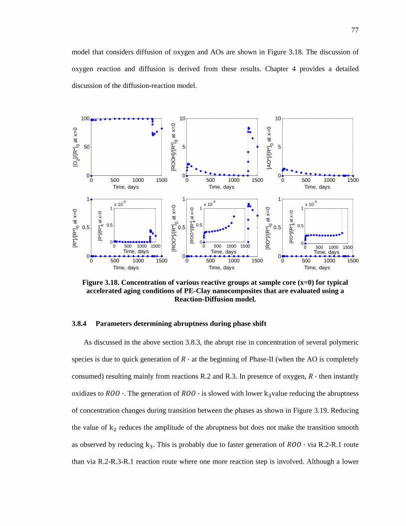
77

model that considers diffusion of oxygen and AOs are shown in Figure 3.18. The discussion of

oxygen reaction and diffusion is derived from these results. Chapter 4 provides a detailed

discussion of the diffusion-reaction model.

Figure 3.18. Concentration of various reactive groups at sample core (x=0) for typical

accelerated aging conditions of PE-Clay nanocomposites that are evaluated using a Reaction-Diffusion model.

3.8.4 Parameters determining abruptness during phase shift

As discussed in the above section 3.8.3, the abrupt rise in concentration of several polymeric

species is due to quick generation of � · at the beginning of Phase-II (when the AO is completely

consumed) resulting mainly from reactions R.2 and R.3. In presence of oxygen, � · then instantly

oxidizes to � ·. The generation of � · is slowed with lower k�value reducing the abruptness

of concentration changes during transition between the phases as shown in Figure 3.19. Reducing

the value of k reduces the amplitude of the abruptness but does not make the transition smooth

as observed by reducing k�. This is probably due to faster generation of � · via R.2-R.1 route

than via R.2-R.3-R.1 reaction route where one more reaction step is involved. Although a lower

0 500 1000 15000

50

100

Time, days

[O2]/

[R*]

0 at

x=0

0 500 1000 15000

0.5

1

Time, days

[R*]

/[R

*]0 a

t x=

0

0 500 1000 15000

0.5

1

Time, days

[RO

O*]

/[R

*]0 a

t x=

00 500 1000 1500

0

5

10

Time, days

[RO

OH

]/[R

*]0 a

t x=

0

0 500 1000 15000

0.5

1

Time, days[R

O*]

/[R

*]0 a

t x=

0

0 500 1000 15000

5

10

Time, days

[AO

*]/[

R*]

0 at

x=0

0 500 1000 15000

0.5

1x 10

-6

Time, days

[R*]

/[R*] 0 a

t x=0

0 500 1000 15000

0.5

1x 10

-6

Time, days

[RO

*]/[R

*] 0 at x

=0

0 500 1000 15000

0.5

1x 10

-6

Time, days

[RO

O*]

/[R*] 0 a

t x=0

78

value of k� makes the transition smoother, a high value of k� is still required in this model to

justify sharp AO depletion in PE-Clay nanocomposites.

Figure 3.19. Concentration of peroxide radical as a function of time for different values of

k2 and k3.

Some free-radical combination reactions are ignored in the model presented in this thesis

because they are insignificant in Phase-I. Therefore, it is possible that some of these ignored

reactions are significant in Phase-II and may smooth out the transition. However when all the

reactions are included in the model, the results show that these ignored reactions are too slow in

Phase-II to reduce the abruptness.

3.8.5 Parametric Study of Termination-II Reactions (R.15 – R.18)

The figures below (Figure 3.20 to Figure 3.23) show �� concentration versus time plots at

different values of rate constants of a particular reaction in each plot while keeping other

parameter constant. The values of rate constants are varied around the best fit value to observe

their sensitivity in affecting �� concentration profiles.

0 500 1000 15000

0.2

0.4

0.6

0.8

1

Time, days

[RO

O.]

/[R*]

0

Abrupt rise with current parameters

lower k2 reduces amplitude of abrupt rise

lower k3 reduces abruptness

79

Figure 3.20 shows that the termination reaction R.15 between � · and � · is significantly able

to alter ���� depletion behavior only when the reaction rate is greater than 109 cm3/mol-s. With

the rate constant k�� = 109 cm3/mol-s, reaction R.15 does not significant affect ���� depletion

behavior since �� ·� is low. However, a higher value of k�� increases the reaction rate and slows

depletion of AO and longer protection of the PE-clay nanocomposites since �� ·� in the reaction

cycle gets lowered.

Figure 3.21 shows that ���� depletion is very sensitive to rates of the termination reaction

R.16 between � · and � ·. This is because the concentration of � · is higher than other

polymeric free radicals thereby increasing the reaction rate. Therefore, the value of k�� is critical

in determining rate of ���� depletion.

Figure 3.22 shows that the termination reaction R.17 between � · and � · is significantly able

to alter ���� depletion behavior only when the reaction rate is greater than 108 cm3/mol-s, quite

similar to the case of reaction R.15 in Figure 3.20. The higher the rate of R.17, the slower is the

���� depletion, since this reduces �� ·�. With rate constant k�� = 109 cm3/mol-s, reaction R.17

only slightly reduces the rate of ���� depletion.

Figure 3.20. Model predictions for $%& concentration for the ‘Base Case’ in Table 3.1 with

varying values of rate constant, k��, that determines the rate of termination reaction between i · and $% ·.

0 200 400 600 800 1000 1200 1400 16000

0.2

0.4

0.6

0.8

1

Time, days

[AO

H]/[

AO

H]

0

0 200 400 600 800 1000 1200 1400 16000

0.2

0.4

0.6

0.8

1

Time, days

[AO

H]/[

AO

H]

0

0 200 400 600 800 1000 1200 1400 16000

0.2

0.4

0.6

0.8

1

Time, days

[AO

H]/[

AO

H]

0

0 200 400 600 800 1000 1200 1400 16000

0.2

0.4

0.6

0.8

1

Time, days

[AO

H]/[

AO

H]

0

0 200 400 600 800 1000 1200 1400 16000

0.2

0.4

0.6

0.8

1

Time, days

[AO

H]/[

AO

H]

0

0 200 400 600 800 1000 1200 1400 16000

0.2

0.4

0.6

0.8

1

Time, days

[AO

H]/[

AO

H]

0

k15

= 1011 cm3/mol-s

k15

= 1010 cm3/mol-s

k15

< 109 cm3/mol-s

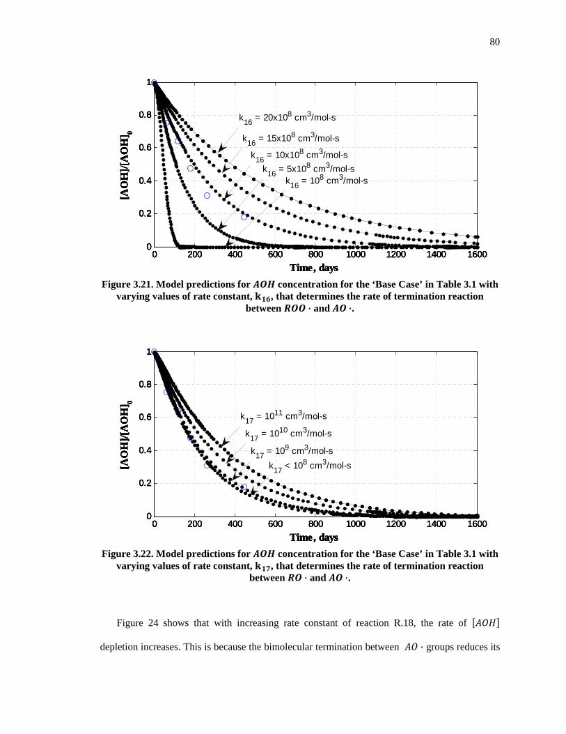
80

Figure 3.21. Model predictions for $%& concentration for the ‘Base Case’ in Table 3.1 with

varying values of rate constant, k��, that determines the rate of termination reaction between i%% · and $% ·.

Figure 3.22. Model predictions for $%& concentration for the ‘Base Case’ in Table 3.1 with

varying values of rate constant, k��, that determines the rate of termination reaction between i% · and $% ·.

Figure 24 shows that with increasing rate constant of reaction R.18, the rate of ���� depletion increases. This is because the bimolecular termination between � · groups reduces its

0 200 400 600 800 1000 1200 1400 16000

0.2

0.4

0.6

0.8

1

Time, days

[AO

H]/[

AO

H]

0

0 200 400 600 800 1000 1200 1400 16000

0.2

0.4

0.6

0.8

1

Time, days

[AO

H]/[

AO

H]

0

0 200 400 600 800 1000 1200 1400 16000

0.2

0.4

0.6

0.8

1

Time, days

[AO

H]/[

AO

H]

0

0 200 400 600 800 1000 1200 1400 16000

0.2

0.4

0.6

0.8

1

Time, days

[AO

H]/[

AO

H]

0

0 200 400 600 800 1000 1200 1400 16000

0.2

0.4

0.6

0.8

1

Time, days

[AO

H]/[

AO

H]

0

0 200 400 600 800 1000 1200 1400 16000

0.2

0.4

0.6

0.8

1

Time, days

[AO

H]/[

AO

H]

0

k16 = 20x108 cm3/mol-s

k16 = 15x108 cm3/mol-s

k16 = 108 cm3/mol-sk16 = 5x108 cm3/mol-s

k16 = 10x108 cm3/mol-s

0 200 400 600 800 1000 1200 1400 16000

0.2

0.4

0.6

0.8

1

Time, days

[AO

H]/[

AO

H]

0

0 200 400 600 800 1000 1200 1400 16000

0.2

0.4

0.6

0.8

1

Time, days

[AO

H]/[

AO

H]

0

0 200 400 600 800 1000 1200 1400 16000

0.2

0.4

0.6

0.8

1

Time, days

[AO

H]/[

AO

H]

0

0 200 400 600 800 1000 1200 1400 16000

0.2

0.4

0.6

0.8

1

Time, days

[AO

H]/[

AO

H]

0

0 200 400 600 800 1000 1200 1400 16000

0.2

0.4

0.6

0.8

1

Time, days

[AO

H]/[

AO

H]

0

k17 = 1011 cm3/mol-s

k17 = 1010 cm3/mol-s

k17 = 109 cm3/mol-s

k17 < 108 cm3/mol-s

81

concentration which in turn reduces its termination rates with other polymeric free radicals.

Therefore, an optimum value of k�� is required to match experimental ���� depletion. The

Figure 3.23 shows that slowest AO depletion is achievable with no termination between � · groups, the higher the reaction rate more detrimental it is for AO depletion. With increasing rate

of reaction R.18, the �� depletion curve changes from exponential decay and asymptotic period

of �� to linear �� depletion.

Figure 3.23. Model predictions for $%& concentration for the ‘Base Case’ in Table 3.1 with

varying values of rate constant, k��, that determines the rate of bimolecular termination reaction within $% ·.

3.8.6 Importance of initial alkyl free radical concentration, �i ·�j

The Figure 3.24 show �� concentration versus time plots at different initial alkyl free

radical concentration, �� ·��. Figure 3.3(d) shows that �� ·� after the initial transient is of the

order of 10-16 mol/cm3, which is 108 times lower than the �� ·�� considered in the model. The high

initial alkyl free radical concentration is quickly oxidized and stabilized by �� during the initial

transient. After this transient, �� ·� accumulated in the reaction cycle R.1-R.10-R.3 is limited to

0 200 400 600 800 1000 1200 1400 16000

0.2

0.4

0.6

0.8

1

Time, days

[AO

H]/[

AO

H]

0

0 200 400 600 800 1000 1200 1400 16000

0.2

0.4

0.6

0.8

1

Time, days

[AO

H]/[

AO

H]

0

0 200 400 600 800 1000 1200 1400 16000

0.2

0.4

0.6

0.8

1

Time, days

[AO

H]/[

AO

H]

0

0 200 400 600 800 1000 1200 1400 16000

0.2

0.4

0.6

0.8

1

Time, days

[AO

H]/[

AO

H]

0

0 200 400 600 800 1000 1200 1400 16000

0.2

0.4

0.6

0.8

1

Time, days

[AO

H]/[

AO

H]

0

0 200 400 600 800 1000 1200 1400 16000

0.2

0.4

0.6

0.8

1

Time, days

[AO

H]/[

AO

H]

0

0 200 400 600 800 1000 1200 1400 16000

0.2

0.4

0.6

0.8

1

Time, days

[AO

H]/[

AO

H]

0

k18 = 102 cm3/mol-s

k18 = 10 cm3/mol-s

k18 = 0

k18 = 104 cm3/mol-s

k18 = 103 cm3/mol-s

k18 = 105 cm3/mol-s

82

about 10-16 mol/cm3 as the rate of the cyclic reactions slow down. Therefore, during the transient

period �� depletes quickly to stabilize almost all initial alkyl free radicals followed by its

slower depletion due to pseudo steady state R.1-R.10-R.3 reaction cycle. This is quite obvious

from Figure 3.24. When the �� ·�� is 10-8 mol/cm3 or less, the initial instant depletion of ���� is

less than 1/837th (or 1.2%) of �����. Therefore, �� ·�� = 10-8 mol/cm3 in the core-model does

not significantly alter the ���� depletion profile.

Figure 3.24. Model predictions for $%& concentration for the ‘Base Case’ in Table 3.1 with

varying values of initial alkyl free radical concentration, �i ·�j, keeping �i����j = 0.

3.8.7 Estimation of initial concentration of various species and influence of �i ·�j and �i����j on AO depletion behavior

During processing, the free radicals generated are oxidized and stabilized by �� and � · thereby generating ��. The generated �� then decomposes to regenerate free radicals in a

cyclic fashion. While being processed in a enclosed system, the oxygen availability is limited to

the amount already dissolved in the polymer. But as soon as it comes out of the extruder or mold,

atmospheric oxygen becomes available. Therefore, there is a fluctuated supply of O2. The

0 200 400 600 800 1000 1200 1400 16000

0.2

0.4

0.6

0.8

1

Time, days

[AO

H]/[

AO

H]

0

0 200 400 600 800 1000 1200 1400 16000

0.2

0.4

0.6

0.8

1

Time, days

[AO

H]/[

AO

H]

0

0 200 400 600 800 1000 1200 1400 16000

0.2

0.4

0.6

0.8

1

Time, days

[AO

H]/[

AO

H]

0

0 200 400 600 800 1000 1200 1400 16000

0.2

0.4

0.6

0.8

1

Time, days

[AO

H]/[

AO

H]

0

0 200 400 600 800 1000 1200 1400 16000

0.2

0.4

0.6

0.8

1

Time, days

[AO

H]/[

AO

H]

0

[R*]0 < 10-8 mol/cm3

[R*]0 = 10-7 mol/cm3

[R*]0 = 10-6 mol/cm3

83

residence time of high temperature processing could be close to a minute, and time taken for the

PE samples to cool down could be 10 minutes for both extrusion and injection processes taken

together.

If it takes 3 years for complete depletion of AO at 85°C, and 70 min at 200°C (in DSC OIT),

then the ratio of AO depletion rates is the ratio these two times. Therefore, AO depletion at 200°C

is about 22,000 times faster than at 85°C. If the processing temperature is close to 200°C, the AO

depleted at a processing time of 2 minutes (approximate equivalence for 1 min. processing and 10

min. cooling) would correspond to AO depleted in about 30 days in the samples at 85°C

considering non-fluctuated and excess supply of O2. With this assumption, to achieve a known

value of AO loss (350 ppm in ‘Comp.1010’, i.e., 11.67%) during processing shown in Figure

3.25, the mathematical simulation show that an initial alkyl free radical concentration of 3×10-8

mol/cm3 is required. This initial concentration of alkyl free radicals corresponds to those that are

generated in the beginning of high temperature processing and not the �� ·��. The �� ·�� is the

concentration of alkyl free radicals left after processing which corresponds to about 2.5×10-8

times 10-8 mol/cm3 = 2.5×10-16 mol/cm3 in Figure 3.26(d). So a value of �� ·�� = 10-8 mol/cm3

used in the core-model is very high when compared to this analysis, although the previous section

shows that even this big �� ·�� do not affect the long term behavior of AO depletion.

Figure 3.25. Predictions for $%& concentration vs. time during processing of ‘Comp.1010’.

0 5 10 15 20 25 30 35 40 45 500.8

0.85

0.9

0.95

1

Time, days

[AO

H]/[

AO

H]

0

0 5 10 15 20 25 30 35 40 45 500.8

0.85

0.9

0.95

1

Time, days

[AO

H]/[

AO

H]

0

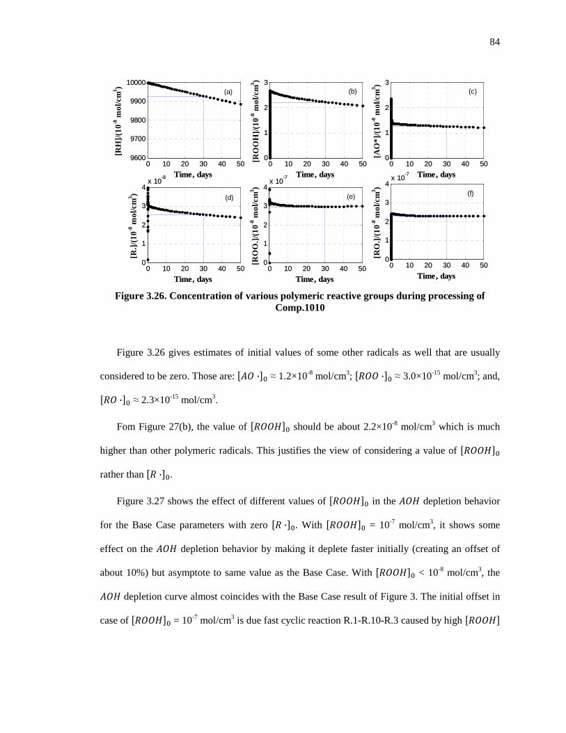
84

Figure 3.26. Concentration of various polymeric reactive groups during processing of

Comp.1010

Figure 3.26 gives estimates of initial values of some other radicals as well that are usually

considered to be zero. Those are: �� ·�� ≈ 1.2×10-8 mol/cm3; �� ·�� ≈ 3.0×10-15 mol/cm3; and,

�� ·�� ≈ 2.3×10-15 mol/cm3.

Fom Figure 27(b), the value of ����� should be about 2.2×10-8 mol/cm3 which is much

higher than other polymeric radicals. This justifies the view of considering a value of �����

rather than �� ·��.

Figure 3.27 shows the effect of different values of ����� in the �� depletion behavior

for the Base Case parameters with zero �� ·��. With ����� = 10-7 mol/cm3, it shows some

effect on the �� depletion behavior by making it deplete faster initially (creating an offset of

about 10%) but asymptote to same value as the Base Case. With ����� < 10-8 mol/cm3, the

�� depletion curve almost coincides with the Base Case result of Figure 3. The initial offset in

case of ����� = 10-7 mol/cm3 is due fast cyclic reaction R.1-R.10-R.3 caused by high ����

0 10 20 30 40 500

1

2

3

4x 10

-8

Time, days0 10 20 30 40 50

0

1

2

3

4x 10

-7

Time, days

0 10 20 30 40 500

1

2

3

Time, days

0 10 20 30 40 500

1

2

3

4x 10

-7

Time, days

0 10 20 30 40 500

1

2

3

Time, days

0 10 20 30 40 500

1

2

3

4x 10

-8

Time, days

[R.]/

(10-8

mo

l/cm

3 )

0 10 20 30 40 500

1

2

3

4x 10

-7

Time, days

[RO

O.]/

(10-8

mo

l/cm

3 )0 10 20 30 40 50

0

1

2

3

4x 10

-7

Time, days

[RO

.]/(1

0-8 m

ol/c

m3 )

0 10 20 30 40 500

1

2

3

Time, days

[AO

*]/(

10

-8 m

ol/c

m3 )

0 10 20 30 40 500

1

2

3

Time, days

[RO

OH

]/(1

0-8 m

ol/c

m3 )

0 10 20 30 40 509600

9700

9800

9900

10000

Time, days0 10 20 30 40 50

9600

9700

9800

9900

10000

Time, days

[RH

]/(1

0-8 m

ol/c

m3 )

(a) (b) (c)

(d) (e) (f)

85

during first 20 days of aging. When compared to experimental results, the model result with a

value of ����� about 10-8 mol/cm3 or less matches the experimental data best.

Figure 3.27. Model predictions for $%& concentration for the ‘Base Case’ in Table 3.1 with

varying values of initial hydroperoxide concentration, �i����j, keeping �i ·�j = 0.

Therefore, although the analysis in this section supports consideration of ����� instead of

�� ·�� but a value of either ����� ≈ 10-8 mol/cm3 or �� ·�� ≈ 10-8 mol/cm3 is able to predict the

experimental �� depletion. Hence, the choice of either ����� or �� ·�� to have a value 10-8

mol/cm3 (or less) is not critical in predicting the long term �� depletion behavior discussed in

this work.

3.9 Conclusions

The core-model presented in this chapter successfully predicts the experimental features of

antioxidant (AO) depletion in PE and PE-clay nanocomposites during the first phase of

degradation (Phase-I) in which AO concentration is significant and prior to the onset of

significant polymer degradation. Prior research has evaluated long term degradation of PE and

PE-clay nanocomposites, but this work pertains to the mechanisms of AO depletion before the

0 200 400 600 800 1000 1200 1400 16000

0.2

0.4

0.6

0.8

1

Time, days

[AO

H]/[

AO

H]

0

0 200 400 600 800 1000 1200 1400 16000

0.2

0.4

0.6

0.8

1

Time, days

[AO

H]/[

AO

H]

0

0 200 400 600 800 1000 1200 1400 16000

0.2

0.4

0.6

0.8

1

Time, days

[AO

H]/[

AO

H]

0

0 200 400 600 800 1000 1200 1400 16000

0.2

0.4

0.6

0.8

1

Time, days

[AO

H]/[

AO

H]

0

0 200 400 600 800 1000 1200 1400 16000

0.2

0.4

0.6

0.8

1

Time, days

[AO

H]/[

AO

H]

0

0 200 400 600 800 1000 1200 1400 16000

0.2

0.4

0.6

0.8

1

Time, days

[AO

H]/[

AO

H]

0

0 200 400 600 800 1000 1200 1400 16000

0.2

0.4

0.6

0.8

1

Time, days

[AO

H]/[

AO

H]

0

0 200 400 600 800 1000 1200 1400 16000

0.2

0.4

0.6

0.8

1

Time, days

[AO

H]/[

AO

H]

0

0 200 400 600 800 1000 1200 1400 16000

0.2

0.4

0.6

0.8

1

Time, days

[AO

H]/[

AO

H]

0

0 200 400 600 800 1000 1200 1400 16000

0.2

0.4

0.6

0.8

1

Time, days

[AO

H]/[

AO

H]

0

0 200 400 600 800 1000 1200 1400 16000

0.2

0.4

0.6

0.8

1

Time, days

[AO

H]/[

AO

H]

0

0 10 20 30 40 500.5

0.6

0.7

0.8

0.9

1

Time, days[A

OH

]/[A

OH

]0

[ROOH]0 < 10-8

[ROOH]0 = 10-7

[ROOH]0 = 10-6

[ROOH]0 = 10-6

86

main PE degradation occurs. During this period, the AO is functional in protecting PE from

oxidative degradation, and the length of this period is a direct indication of its service lifetime.

To model AO depletion in neat PE, the majority of the parameters were obtained from the

literature, and the only adjustable parameter was the termination rate constant k16 to account for

differences in reactivity of the antioxidants used in the experiments. To model AO depletion in

nanocomposites, only one parameter was modified from those used as in neat PE; the

hydroperoxide decomposition rate constant (k�� ) was adjusted to match the initial slope of AO

depletion observed experimentally.

The core-reaction model for AO depletion in PE and PE nanocomposites qualitatively

predicts some important features of experimentally-observed AO depletion. There is small AO

depletion in neat PE until about 500 days of aging due to slow generation of free radicals, and

global phenolic group concentration in AO hundreds of times larger than the initial free radical

concentrations. However, in the nanocomposites, the AO depletion is faster due to accelerated

�� decomposition, which causes cyclic generation of free radicals and depletion of AO.

Several possible mechanisms for accelerated �� decomposition in nanocomposite PE are

possible. Both � · and � · are stabilized by AO which converts them to �� and ��.

The regenerated �� then again decomposes to continue the AO depletion cycle. As long as

AO concentration is high, the rate of this reaction cycle is nearly constant causing the

experimentally-observed linear depletion of AO in the nanocomposites during the first 100 days

of aging.

Free radical termination reactions with phenoxyl radicals (� ·) inhibit the growth of � · and � · causing phenolic groups in AO to deplete following an approximate first order

kinetics. Therefore with an approximate exponential depletion in AO, the slope of AO

concentration versus time changes smoothly from linear to asymptotic. When the termination

87

reaction by � · is more rapid, as in the Case of Irganox 1076, AO depletion rates diminish more

rapidly and the service life of the polymer nanocomposites is extended.

Fast �� decomposition is found to be the root cause of severe AO depletion. Therefore,

for long service lifetime of the nanocomposites, a transition of research is needed to develop

antioxidants that stabilize free radicals without generating �� or that stabilize ��. Also,

there is need for better experimental kinetic data to predict the key degradation reactions.

The core AO depletion model discussed in this chapter did not consider diffusion of O2 and

AO, which can significantly affect the distribution of AO and various other reactive species

throughout the depth of the samples. The next chapter presents a model that includes both

reaction and diffusion mass transfer.

88

CHAPTER 4: REACTION-DIFFUSION MODEL DESCRIBING ANTIOXIDANT DEPLETION THROUGHOUT THE SAMPLE DEPTH

4.1 Introduction

The rate of oxidative degradation of a thick polymer sample depends on the rates of diffusion

of oxygen to its interior, the rates of free radical degradation reactions, and the rate of

stabilization of free radicals by reacting with AO. Low molecular weight molecules, such as O2

and AO molecules move relatively easily through the polymer by diffusion. AO can migrate to

the polymer surface and exit the polymer by evaporation, washing out by water or solvent, or

surface crystallization[63]. Therefore, diffusion of O2 and AO can significantly affect the

distribution of different reactive species throughout the depth of the samples. The earliest work

on reaction and diffusion models to describe polymer oxidation appears in 1980s [30] which were

based on constant initiation rate of alkyl free radicals. However, a constant free radical initiation

assumption is not justified for thermo-oxidative degradation. This chapter describes a model that

considers the reaction scheme analyzed in Chapter 3, O2 diffusion from surroundings to the

sample core, and AO diffusion from core to the surface where it can evaporate to the

surroundings. The model also describes that several factors including spatial variations in clay

orientation that can cause severe AO depletion in a surface layer of the PE-clay nanocomposites.

The overall goal of this research is to investigate reactions and diffusion of various reactive

chemical species in pure PE and PE-clay nanocomposites and propose mathematical models to

match experimental features of AO depletion behavior. In this chapter also, experimental

‘oxidation induction time’ (OIT) data showing variation in depletion with depth through the

sample has guided development of the model [19]. OIT is an indirect measure of active AO

concentration present in a polymeric sample. Two types of AOs are studied in this chapter:

Irganox-1010 and Irganox-1076. These are primary AOs with organic molecules containing

hindered phenol that stabilize peroxide and oxide radicals as described in Chapter 2, section 2.2.6.

89

During the experiments conducted by collaborators on this research, PE-clay nanocomposite

samples were held at 85°C in a circulated air atmosphere. The thicknesses of the samples are

about 3 mm. In thick PE-clay nanocomposite samples, two zones of AO depletion are observed: a

‘flat core zone’ and ‘depleted skin zone’ as shown in Figure 4.2. In the ‘flat core zone’ AO

depletion is slower and uniform. In the ‘depleted skin zone’, AO depletes more rapidly.

This chapter utilizes the reaction kinetic scheme as in Chapter 3 together with physical loss of

AO through the sample surface which depends on AO diffusivity, its saturation concentration and

rate of evaporation to surrounding atmosphere. Free radicals and PE molecular chains are

considered immobile with respect to smaller molecules of O2 and ��. Therefore, free radical

concentrations depend on chemical reactions only. In the ‘flat core zone’ AO depletion is mainly

due to the chemical reactions, but in the ‘depleted skin zone’ severe AO depletion can be caused

by its rapid reaction with free radicals together with physical loss and reduced diffusivities of O2

and AO in the skin due to clay orientation.

4.2 Model Equations and Assumptions

The mathematical model in this chapter predicts O2 and phenolic group (��) concentration

profiles through the depth of sample at different aging times and concentration profiles for other

reacting species as well. Although AO consist of both �� and �· groups, AO concentration is

approximately same as �� concentration because [�·] is always predicted to be over 100

times less than ����. In accelerated aging experiments that are modeled in this research, the

typical sample size is 17.20cm × 2.53cm × 0.32cm[19]. Because both lateral surfaces of the

polymer are exposed to air and the thickness is small compared to the lateral dimensions, a

transient one-dimensional model is appropriate as depicted in Figure 4.1. The sample is

symmetric about the central line which is considered at ! g 0, and the exposed surfaces are at

! g �o. The surfaces are exposed to circulated air at 85°C which supplies O2 to the sample-

surface. �� can diffuse towards surface and evaporate. The rate of evaporation can be enhanced

90

by circulation of air around samples. Little is known about properties of the phenoxyl radical,

�·, so it will be assumed that it diffuses in a similar way as �� with no evaporation at the

surface. Surface evaporation is neglected because [�·] is predicted to be about 1000 times lower

than �AOH��, which creates a negligible concentration gradient across the surface.

Figure 4.1. Schematic diagram of PE (a), and PE-clay (b) samples showing one-dimensional coordinate system. The diameter of spherulites in PE and length of clay particles are in the

same order. The clay particles orient themselves along the edges of the samples.

4.2.1 Oxygen Transport and Reaction

The reactions pertaining to AO depletion has been discussed in Chapter 2. All reactions in

Chapter 2, Table 2.1 are assumed to be homogeneous, where �� is the effective reaction rate

constant for reaction R.i where subscript i represents the respective reaction number. In a planar

sample, the oxygen concentration varies in only one direction, !, perpendicular to its surface (as

shown in Figure 4.1). The evolution of oxygen concentration is described by the following

diffusion and reaction equation:

�� ��f g �

�! ���?�� �

�! � J ���� ·�� � J ��������� � 4.1

x = + l

x = 0

x = − l

Composite O2

O2

AOH

AOH

R• + O2 → ROO• ROO• + AOH → ROOH +AO• ROOH + RH → R• + RO• + H2O RO• + AOH → ROH +AO•

(b)

x x

(a)

x = + l

x = 0

x = − l

Neat PE O2

O2

AOH

AOH

R• + O2 → ROO• ROO• + AOH → ROOH +AO•

91

where, � � is oxygen concentration, and ��? is effective oxygen diffusivity in the polymer

matrix.

Initially, the oxygen concentration inside the sample is assumed to be negligible:

� ���� g 0 4.2

O2 enters the sample through the lateral surfaces (! g �o) and is consumed by reactions R.0 and

R.1. In diffusion calculations it can be assumed that the oxygen concentration on the sample

surface is equal to the product of the partial oxygen pressure and the coefficient of solubility,  

(Henry’s Law) which does not vary during the reaction. Actual experimental values of O2

solubility in pure PE at different temperatures are also available in literature and a typical value is

reported in Table 2.2.

� �]¡�¢^ g   � £�? 4.3

The oxygen concentration varies in the !-direction and is symmetric about ! g 0. At the center of

a sample oxygen flux is zero, i.e.:

J�� ¤�� ��! ¥

¡��g 0 4.4

4.2.2 Antioxidant Transport and Degradation

Antioxidants in PE can be depleted by a combination of physical and chemical losses.

Physical losses include evaporation, washing and/or adsorption within or onto clay layers and

chemical losses occur by reactions described in Chapter 2. The overall mass balance on ��

produces the diffusion-reaction equation given by Equation 4.5.

92

������f g �

�! ��¦������

�! � J k���� ·����� J k���� ·�����- k�M������ ·�

4.5

where ���� is the concentration of phenolic group, and �¦� is the effective diffusivity of ��.

The initial �� concentration is uniform throughout the sample thickness.

����§� ��� g ����� 4.6

The model is symmetric about, ! g 0, so the flux of �� is zero at the center:

¤������! ¥

¡��g 0 4.7

Because �� is a relatively small molecule, it can diffuse to the surface and evaporate. The rate

of diffusion to the surface equals the rate of evaporation using a mass transfer coefficient.

J�¦� ¤������! ¥

¡�¢g �¨©�u����¡�¢ J ����¨ªv 4.8

where, �¨© is a mass transfer coefficient for �� evaporation based on the ���� at the surface,

� is ratio of saturated ���� in samples to saturated ���� in surrounding air, and ����¨ª is

the equilibrium concentration of the �� in the gas/air layer surrounding sample surface.

Generally, ����¨ª is negligible due to air convection through the oven. The mathematical form

of the evaporation boundary condition (Equation 4.8) is modified in the cases predicting

blooming discussed later in section 4.4.1.

The phenoxyl groups in AO, ��, stabilizes a free radical by donating a proton and

transforms to a comparatively stable phenoxyl group, � ·. The overall mass balance on � · produces the diffusion-reaction equation:

93

��� ·��f g �

�! ��¦������

�! � - k���� ·����� - k���� ·����� J k�������� ·�J k�M������ ·� J k���� ·��� ·� J k���� ·��� ·�J k���� ·��� ·� J 2k���� ·�

4

.9

Where �� ·� represents concentration of phenoxyl radicals. The diffusivity of phenoxyl radicals

are considered to be the same as of phenolic groups. Initially, �� ·� is set to zero. The flux of

� · is zero at the center is given by:

¤��� ·��! ¥

¡��g 0 4.10

For the sake of simplicity, � · evaporation from the sample surface is neglected. In the

present case the concentration of � · is expected to be of the order of polymeric reactive species

concentrations that are about 1000 times smaller than �����. With no physical loss of � · at

sample surface, its flux at x=1 is given by:

¤��� ·��! ¥

¡�¢g 0 4.11

4.2.3 Reactions of Polymer Species

Diffusion of the reactive polymer species is insignificant because their diffusion coefficients

are on the order of 10-18 cm2/s. Although the polymer species are immobile they do develop

concentration profiles due to reaction with non-uniform � � and ����. The concentration of

alkyl groups, ����, is about 105 times higher than all the free radicals (Table 2.3) and is,

therefore, expected to be fairly constant. The governing equations for the evolution of the reactive

polymeric species remains the same as mentioned in Chapter 3 and are summarized in Table 4.1

below.

94

Table 4.1. Summary of equations governing the evolution of various polymeric reactive species

Eq.# Equations for Polymeric Reactive Groups

3.3 d�� ·�

df g Jk��� ·��O �cde - k �� ·����� - k��������� - kM�� ·����� - k��� ·�- k�������� ·� J k���� ·��� ·�

3.4 d�� ·�

df g k��� ·��O �cde J k �� ·����� J 2k��� ·� J k���� ·�����- k�M������ ·� J k���� ·��� ·�

3.5 d����df g Jk�������O �cde J k �� ·����� J k������ J kM�� ·����� J k�������� ·�

3.6 d����

df g k�������O �cde - k �� ·����� J k������ - k���� ·�����J k�������� ·�

3.7 d�� ·�

df g k������ J kM�� ·����� J k��� ·� J k���� ·����� J k���� ·��� ·� .

In the Table 4.1, �� ·� is the concentration of alkyl free radical which is initially �� ·��.

�� ·� and �� ·� are concentrations of peroxide free radical and alkoxy free radicals

respectively which are negligible initially. ���� represents alkyl-hydroperoxide concentration

and is initially set to zero. The concentration profiles of these polymer species mainly depend on

oxidation of alkyl radicals, �� concentration, and their reaction rates. Table 3.1 in Chapter 3

shows the values of various reaction rate constants considered in the model.

4.2.4 Numerical Method of Solution

The partial and ordinary differential equations (PDEs & ODEs) in the model were solved

numerically using the initial and boundary conditions. The finite difference method was used to

convert the PDEs into a set of ODEs. The domain was divided into 100 equally spaced intervals

over which finite difference equations were used to approximate spatial derivatives. The set of

ODEs were then solved simultaneously using a stiff ODE solver in MATLAB. (The MATAB

code can be found in Appendix A.) The computer used for these calculations was a Dell

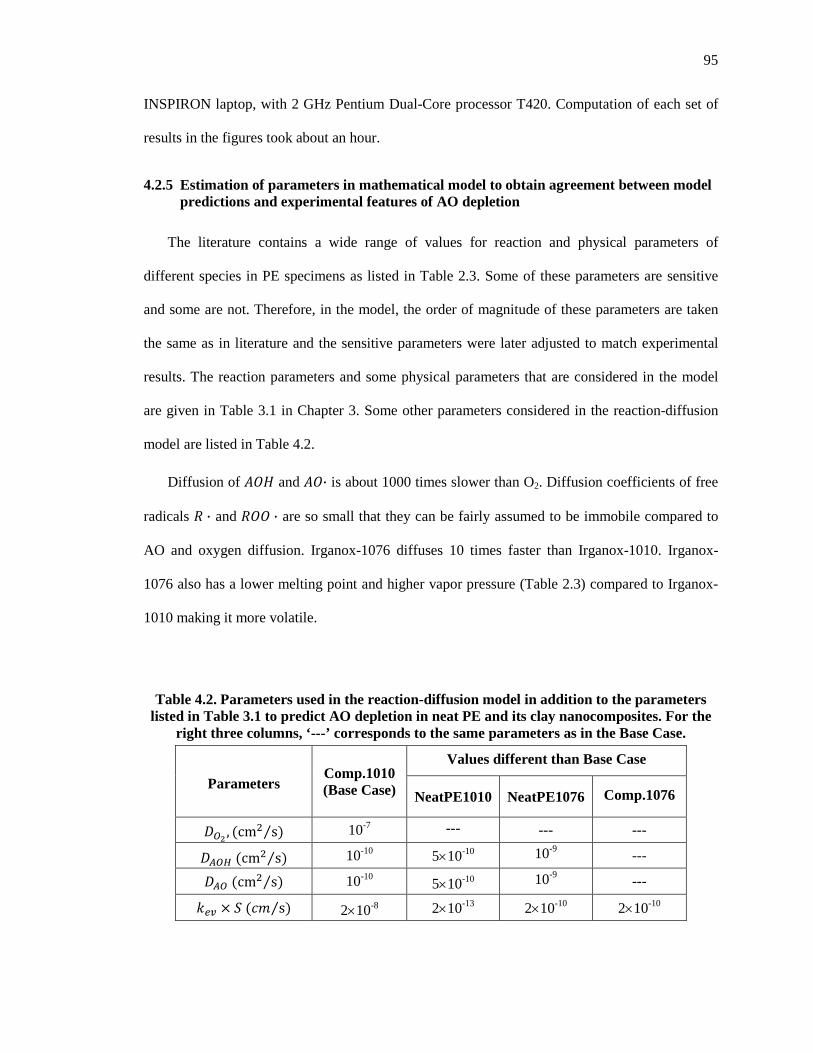
95

INSPIRON laptop, with 2 GHz Pentium Dual-Core processor T420. Computation of each set of

results in the figures took about an hour.

4.2.5 Estimation of parameters in mathematical model to obtain agreement between model predictions and experimental features of AO depletion

The literature contains a wide range of values for reaction and physical parameters of

different species in PE specimens as listed in Table 2.3. Some of these parameters are sensitive

and some are not. Therefore, in the model, the order of magnitude of these parameters are taken

the same as in literature and the sensitive parameters were later adjusted to match experimental

results. The reaction parameters and some physical parameters that are considered in the model

are given in Table 3.1 in Chapter 3. Some other parameters considered in the reaction-diffusion

model are listed in Table 4.2.

Diffusion of �� and �· is about 1000 times slower than O2. Diffusion coefficients of free

radicals � · and � · are so small that they can be fairly assumed to be immobile compared to

AO and oxygen diffusion. Irganox-1076 diffuses 10 times faster than Irganox-1010. Irganox-

1076 also has a lower melting point and higher vapor pressure (Table 2.3) compared to Irganox-

1010 making it more volatile.

Table 4.2. Parameters used in the reaction-diffusion model in addition to the parameters listed in Table 3.1 to predict AO depletion in neat PE and its clay nanocomposites. For the

right three columns, ‘---’ corresponds to the same parameters as in the Base Case.

Parameters Comp.1010 (Base Case)

Values different than Base Case

NeatPE1010 NeatPE1076 Comp.1076

��? , ]cm s⁄ ^ 10-7 --- --- ---

�¦�« ]cm s⁄ ^ 10-10 5×10-10 10-9 ---

�¦� ]cm s⁄ ^ 10-10 5×10-10 10-9 ---

�¨© � � ]¬­ s⁄ ^ 2×10-8 2×10-13 2×10-10 2×10-10

96

Neat PE samples are modeled using parameters found in the literature. In case of

nanocomposites, some of the parameters (k3, k16, kev) were adjusted to achieve qualitative

agreement between model predictions and experimentally-measured AO profiles. The parameters

for various cases are listed in italics in Table 3.1 and Table 4.2.

4.3 Results & Discussions

4.3.1 Model Predictions for a base case ‘Comp.1010’

The reaction and diffusion model predicts profiles of oxygen, ��, �·, and polymer

species as a function of depth in the samples and as a function of time. Typical results for a base

case are shown in Figure 4.2 and Figure 4.3. Conditions used for these results are same as for PE-

Clay nanocomposites with Irganox-1010, which are listed in Table 4.2 under the column ‘Comp.

1010’.

Figure 4.2. Concentration profiles of (a) O2 and (b) $%&, predicted by the model for typical accelerated aging conditions of Comp.1010. The parameters used for this figure correspond

to ‘Base Case’ in Table 4.2.

0 0.2 0.4 0.6 0.8 10

0.2

0.4

0.6

0.8

1

x

[O2](

x,t)

/[O

2] sat

0 0.2 0.4 0.6 0.8 10

0.2

0.4

0.6

0.8

1

x

[AO

H](

x,t)

/ [

AO

H]

0

(a)

0 day

30 daysand above

withincreasingtime

90 days

180 days

270 days

360 days

450 days

(b)

0 day

97

Figure 4.3. Concentration profiles of various polymeric species for typical accelerated aging

conditions of PE-Clay nanocomposites ‘Base Case’ for same times as in Figure 4.3.

Figure 4.4. Concentration profiles of $%& for the cases of (a) no evaporation, (b) no reaction, and (c) 10 times faster $%& diffusion than typical case of Figure 4.2(b).

O2 and �� concentration profiles are shown in Figure 4.2(a) and Figure 4.2(b), and the

profiles for polymeric species are shown in Figure 4.3. The profiles vary along the depth of the

0 0.5 10

0.2

0.4

0.6

0.8

1

x

[R*]

/[R

*]0

0 0.5 10

2000

4000

6000

8000

10000

x

[RH

]/[R

*]0

0 0.5 10

0.2

0.4

0.6

0.8

1

x

[RO

O*]

/[R

*]0

0 0.5 10

0.5

1

1.5

2

x

[RO

OH

]/[R

*]0

0 0.5 10

0.2

0.4

0.6

0.8

1

x

[RO

*]/[

R*]

0

0 0.5 10

0.5

1

1.5

2

x

[AO

*]/[

R*]

0

0 0.5 10

2

4

6x 10

-7

0 0.5 10

1

2

3x 10

-7

0 0.5 10

0.5

1x 10

-7

withincreasingtime

withincreasingtime

(a) (b) (c)

(d) (e) (f)

30 days & above

0 0.5 10

0.2

0.4

0.6

0.8

1

x

[AO

H]

/ [A

OH

] 0

(c)

30 days

90 days

180 days

0 0.5 10

0.2

0.4

0.6

0.8

1

x

[AO

H]

/ [A

OH

] 0

(b)

445days

30days

0 0.5 10

0.2

0.4

0.6

0.8

1

x

[AO

H]

/ [A

OH

] 0

(a)

30 days

445 days

98

sample, !, which is scaled with o to give ! g 0 at the sample core and ! g 1 at sample surface.

O2 concentration is normalized by the oxygen solubility in PE, � �®; so, � � � �®⁄ is initially

zero everywhere but rapidly rises to � � � �®⁄ ¯ 1. �� concentration is normalized by the

initial �� concentration; so it is initially uniform at ���� �����⁄ g 1. The polymer species

are scaled with initial � · group concentration. The concentrations of most of the polymer species

vary between zero to about 10-8 mol/cm3 which after the scaling becomes 1 as shown in Figure

4.3. The ratios of scaling factors of �� (Irganox-1010) and O2 to scaling factor of polymer

species are ����� �� ·��⁄ g 875, and � �® �� ·��⁄ g 100. Therefore, a change of 1 scaled

value of alkyl free radical corresponds to a change of 1.14×10-3 scaled value of �� (Irganox-

1010) and 1×10-2 scaled value of O2. Since a negligible amount of �� is consumed by the initial

�� ·�, depletion of �� requires either formation of new free radicals or a cyclic reaction to

consume �� described in Section 3.4.

Figure 4.4 shows how the �� profiles for three cases in which the model parameters were

modified to demonstrate sensitivity of the predictions to specific mechanisms. In the ‘no

evaporation’ condition of Figure 4.4(a), the �� depletion is mainly due to reactions with � · and � ·, and the predicted �� concentration decreases in accordance to core �� depletion

described in Chapter 3. In the ‘no reaction’ condition of Figure 4.4(b), the depletion is only by

evaporation, and the predicted �� concentration shows a steep gradient towards the surface and

minimal depletion at the core. Also, the depletion in the core of the “no reaction” case is more

parabolic, whereas the core depletion with reaction in Figure 4.2(b) shows a flat ��

concentration profile in the center (which decreases with time as in the core model of Chapter 3).

Therefore, the core �� depletion in Figure 4.2(b) appears to be a sum of the losses due to the

reactions and surface evaporation. The steepness of the �� gradient near the surface is strongly

affected by the �� diffusivity as demonstrated by Figure 4.4(c) in which the �� diffusivity is

99

increased by a factor of ten, and the �� replenishment from sample core causes a much

shallower �� profiles.

Figure 4.5. Total Oxygen and $%& during first 90 days for typical aging conditions of the

‘Base Case’.

Changes in the total amounts of O2 and �� in the sample during early times are shown in

Figure 4.5. It takes about 10 days for O2 to achieve steady state, while the depletion of �� is

approximately linear with roughly 40% depletion after 90 days aging at 85°C. O2 and � · profiles

in Figure 4.2(a) and Figure 4.3(d) respectively also show that oxygen, after reacting with all � · in

less than 30 days, uniformly distributes throughout the polymer close to its saturation point. Slow

propagation reactions R.2, R.4, R.6 and R.13 provide slow generation of � ·, which immediately

oxidizes lowering the O2 concentration by about 2% from its saturation value. Slow propagation

reactions R.2, R.3, R.4 and R.13 cause gradual decrease in ����� in Figure 4.3(a).

0 10 20 30 40 50 60 70 80 900

0.1

0.2

0.3

0.4

0.5

0.6

0.7

0.8

0.9

1

[AO

H]/

[AO

H]

0

0

0.1

0.2

0.3

0.4

0.5

0.6

0.7

0.8

0.9

1

Time, days

[O2]/

[O2] sa

t

Total [O2]

Total [AOH]

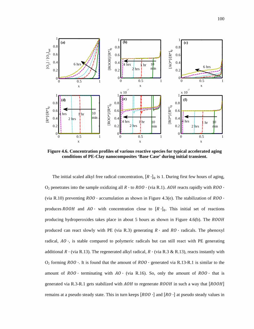
100

Figure 4.6. Concentration profiles of various reactive species for typical accelerated aging

conditions of PE-Clay nanocomposites ‘Base Case’ during initial transient.

The initial scaled alkyl free radical concentration, �� ·�� is 1. During first few hours of aging,

O2 penetrates into the sample oxidizing all � · to � · (via R.1). �� reacts rapidly with � · (via R.10) preventing � · accumulation as shown in Figure 4.3(e). The stabilization of � · produces �� and � · with concentration close to �� ·��. This initial set of reactions

producing hydroperoxides takes place in about 5 hours as shown in Figure 4.6(b). The ��

produced can react slowly with PE (via R.3) generating � · and � · radicals. The phenoxyl

radical, � ·, is stable compared to polymeric radicals but can still react with PE generating

additional � · (via R.13). The regenerated alkyl radical, � · (via R.3 & R.13), reacts instantly with

O2 forming � ·. It is found that the amount of � · generated via R.13-R.1 is similar to the

amount of � · terminating with � · (via R.16). So, only the amount of � · that is

generated via R.3-R.1 gets stabilized with �� to regenerate �� in such a way that ���� remains at a pseudo steady state. This in turn keeps �� ·� and �� ·� at pseudo steady values in

0 0.5 10

0.2

0.4

0.6

0.8

1

x

[RO

OH

]/[R

*]0

0 0.5 10

0.2

0.4

0.6

0.8

1

x

[AO

*]/[

R*]

0

0 0.5 10

0.2

0.4

0.6

0.8

1

x

[R*]

/[R

*]0

0 0.5 10

0.2

0.4

0.6

0.8

1x 10

-7

x

[RO

O*]

/[R

*]0

0 0.5 10

0.2

0.4

0.6

0.8

1x 10

-7

x

[RO

*]/[

R*]

0

0 0.5 10

0.2

0.4

0.6

0.8

1

x

[O2]

/ [

O2]

sat

(a)

(d)

(b) (c)

(f)(e)

6 hrs6 hrs

10min

1 hr

2 hrs

4 hrs

10min

10min

10min

1 hr 1 hr4 hrs 4 hrs

1 hr4 hrs

2 hrs

2 hrs 2 hrs

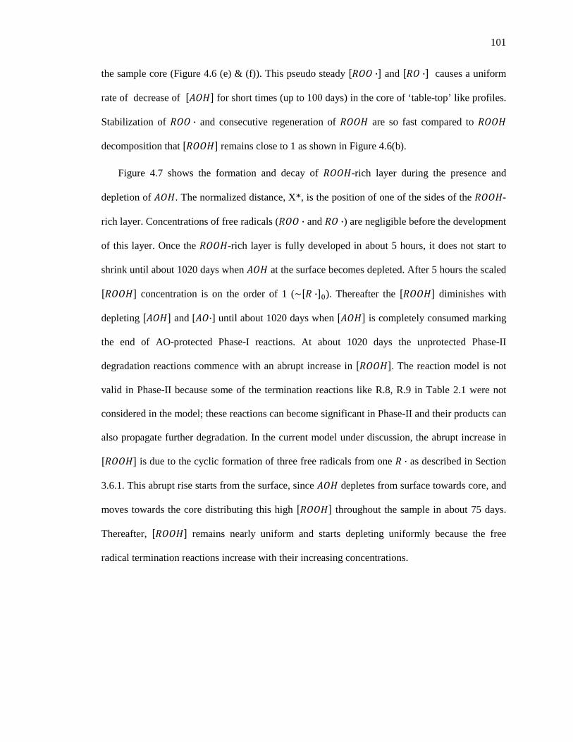
101

the sample core (Figure 4.6 (e) & (f)). This pseudo steady �� ·� and �� ·� causes a uniform

rate of decrease of ���� for short times (up to 100 days) in the core of ‘table-top’ like profiles.

Stabilization of � · and consecutive regeneration of �� are so fast compared to ��

decomposition that ���� remains close to 1 as shown in Figure 4.6(b).

Figure 4.7 shows the formation and decay of ��-rich layer during the presence and

depletion of ��. The normalized distance, X*, is the position of one of the sides of the ��-

rich layer. Concentrations of free radicals (� · and � ·) are negligible before the development

of this layer. Once the ��-rich layer is fully developed in about 5 hours, it does not start to

shrink until about 1020 days when �� at the surface becomes depleted. After 5 hours the scaled

���� concentration is on the order of 1 (~�� ·��). Thereafter the ���� diminishes with

depleting ���� and [�·] until about 1020 days when ���� is completely consumed marking

the end of AO-protected Phase-I reactions. At about 1020 days the unprotected Phase-II

degradation reactions commence with an abrupt increase in ����. The reaction model is not

valid in Phase-II because some of the termination reactions like R.8, R.9 in Table 2.1 were not

considered in the model; these reactions can become significant in Phase-II and their products can

also propagate further degradation. In the current model under discussion, the abrupt increase in

���� is due to the cyclic formation of three free radicals from one � · as described in Section

3.6.1. This abrupt rise starts from the surface, since �� depletes from surface towards core, and

moves towards the core distributing this high ���� throughout the sample in about 75 days.

Thereafter, ���� remains nearly uniform and starts depleting uniformly because the free

radical termination reactions increase with their increasing concentrations.

102

Figure 4.7. Depth of �� rich layer developed in presence of $%& (a) and during absence

of $%& when actual PE degradation starts (b).

4.3.2 Comparison of Core-Reaction Model with Diffusion-Reaction Model

Figure 4.8 compares concentrations of various reactive groups for typical accelerated aging

conditions of the base case ‘Comp.1010’ at sample core obtained by the Core-Reaction Model of

Chapter 3 (black line without marker) and by the Diffusion-Reaction Model (blue line with

marker) with the evaporative boundary condition for ��. In the core-reaction model described

in Chapter 3, the oxygen concentration was considered uniform at all times. The predictions from

reaction and diffusion model in Figure 4.8(a) shows this to be true for most of the Phase-I.

However, during the transition from Phase-I to Phase-II, [O2] starts to diminish at around 1020

days of aging until it reduces to a minimum of about 70% of [O2]sat at about 1200 days. This

reduction in [O2] is because of increased oxidation rate with increased generation of alkyl free

radicals, � ·. After 1020 days, the ���� reduces below 1% of its initial concentration causing

� · and � · to increase as shown in the insets of Figure 4.8(e) and Figure 4.8(f). With

increasing � ·, its β-transition increases generation of the � ·. The increased generation of � · continues until the end of Phase-I at about 1200 days. At the beginning of Phase-II the model

predicts a sudden rise in �� ·� because all � · now reacts with weak points in PE molecule, ��.

0 5 10 150

0.1

0.2

0.3

0.4

0.5

0.6

0.7

0.8

0.9

1

Time, hrs

X*,

Sca

led

dist

ance

of m

ovin

g fr

ont

of R

OO

H

800 900 1000 1100 1200 13000

0.1

0.2

0.3

0.4

0.5

0.6

0.7

0.8

0.9

1

Time, days

X*,

Sca

led

dist

ance

of m

ovin

g fr

ont

of R

OO

H

0 0.5 10

5

10

x

[RO

OH

]/[R

*]0

0 0.5 10

0.5

1

x

[RO

OH

]/[R

*]0

IncreasingTime

AOH & AO* active instabilizing ROO*

Initially, ROOH ~ [R*]0 but

gradually deminishes

(b)(a)

Increasing T ime

RO* ~ 0ROO* ~ 0R* ~ [R*]

0

AOH & AO* depleted

ROOH rises abruptlyand then deminishes

103

As time progresses further, ���� reduces diminishing � · generation, and [O2] at sample core

increases.

A constant [O2] assumption in the core reaction model, causes a faster oxidation reaction

(R.1) during the transition from Phase-I to Phase-II giving less accumulation of �� ·� compared to

diffusion-reaction model. With lower �� ·� in core-reaction model, its termination reaction (R.15)

with � · is also slower, causing an longer life of � ·. This in turn causes a delay in the abrupt

change of concentrations of polymeric species shown in Figure 4.8. So, interestingly, under the

conditions of this model, lower oxygen concentration at the end of Phase-I reduces the length of

time of the protected Phase-I by about 100 days.

Figure 4.8. Comparison of concentrations of various reactive groups at sample core for

typical accelerated aging conditions of PE-Clay nanocomposites ‘Base Case’ obtained by Core-Reaction Model and by Diffusion-Reaction Model: (a) oxygen %°, (b) hydroperoxides i%%&, (c) phenoxyl radicals $% ·, (d) alkyl radicals i ·, (e) peroxide radicals i%% ·, and, (f) alkoxy radicals i% ·. All concentrations are normalized by the initial alkyl free radical

concentration, �i ·�j.

0 500 1000 15000

20

40

60

80

100

120

Time, days

[O2]

/[R

*]0

at x

=0

0 500 1000 15000

1

2

3

4x 10

-7

Time, days

[R*]

/[R

*]0

at x

=0

0 500 1000 15000

0.2

0.4

0.6

0.8

1

Time, days

[RO

O*]

/[R

*]0

at x

=0

0 500 1000 15000

2

4

6

8

Time, days

[RO

OH

]/[R

*]0

at x

=0

0 500 1000 15000

0.2

0.4

0.6

0.8

1x 10

-4

Time, days

[RO

*]/[

R*]

0 at

x=

0

0 500 1000 15000

0.5

1

1.5

Time, days

[AO

*]/[

R*]

0 at

x=

0

Diff-Rxn ModelCore Rxn Model

0 500 1000 15001.5

2

2.5

3

3.5x 10

-7

Diff-Rxn Model

Core Rxn Model

0 500 1000 15000

1

2

3x 10

-6

0 500 1000 15000

0.5

1x 10

-8(d)

(b) (c)

(f)(e)

(a)[O2]sat/[R*] 0

104

4.3.3 Significance of oxygen diffusion

The free radical oxidation reaction (R.1) is very fast compared to O2 diffusion but the amount

of free radical is on the order of 10-16 cm3/mol-s. When the model equations were scaled, the non-

dimensional ratio of oxidation rate and O2 diffusion rate is a Damkohler number g��o �� ·� �� ⁄ . Here �� = 109 cm3/mol-s, o = 0.16 cm, �� = 10-7 cm2/s and �� ·� varies between

0.5×10-16 to 2.2 ×10-16 mol/cm3 as given by the inset of Figure 4.3(d). So, the value of Damkohler

number varies between 0.01 and 0.05 for most of Phase-I. This means that oxygen diffusion rate

dominates over oxidation rate due to the limited amount of alkyl free radicals (�·) present in the

samples. Generation of �· depends on R.1-R.10-R.3 cycle which is controlled by R.3

(hydroperoxide decomposition). It takes about 5 hours to oxidize all initial � · (which is the same

as formation time for the fully developed ��-rich layer in Figure 4.6(b), and also same as the

time taken by O2 to penetrate to sample core as shown in Figure 4.6(a)). Once all alkyl free

radicals are oxidized, oxygen diffuses into the sample and uniformly distributes throughout it.

Generation of � · due to the propagation reactions R.2 and R.4 is negligible. There is a slow

generation of � · due to slow decomposition of �� (R.3) in the composite samples. This

lowers the O2 concentration only by about 2% from its saturation value at the sample core. Thus,

oxygen diffusion is not a limitation in determining �� depletion behavior.

4.4 Comparison of Model to Accelerated Aging Experiments

In this section, predictions from the model are compared to results from accelerated aging

experiments. The experimental results discussed in this chapter include samples whose

compositions are discussed in Chapter 3, section 3.7 and displayed in Table 3.4. The preparative

methods and techniques are described elsewhere[19]. The samples described are neat PE with

Irganox-1010 (Neat PE 1010), PE-clay composite with Irganox-1010 (Comp. 1010), neat PE with

Irganox-1076 (Neat PE 1076), and PE-clay composite with Irganox-1076 (Comp. 1076)

respectively. The method used to obtain OIT profiles as a function of sample depth is described in

105

detail elsewhere[19] and is depicted in Figure 1.3(b) of Chapter 1. In this method, an

approximately 3mm thick sample is sliced into several layers and each of the individual slices

were then subjected to OIT test. AO concentration is expected to be linearly proportional to OIT

[23, 83]. To obtain OIT profiles as a function of time, the samples were tested at different aging

times.

The experimental OIT of individual slices of a sample gave an OIT profile throughout the

depth. OIT of each slice is, therefore, a representation of average AO concentration over its

thickness. To compare this average OIT of each slice with the model results, the predicted AO

concentration profiles are divided into the corresponding number of slices and the concentration

is averaged over the thickness of each slice.

Figure 4.10, Figure 4.11, and Figure 4.13 in this section compare various AO profiles

predicted by the model with experimentally determined OIT profiles for different samples of neat

PE and PE-clay nanocomposites. The results are for three different operating environments at

85°C: forced air, stagnant nitrogen, and stagnant air. Under different operating conditions,

different AO profiles are observed, such as (1) ‘blooming’, (2) ‘table-top’ and (3) ‘no core

depletion’. The following paragraphs discuss the comparison of these experimental observations

and model predictions. To predict the experimental features, some model parameters such as O2

and AO diffusivities, rate constant of �� decomposition, and AO partition coefficient were

adjusted as listed in Table 4.2.

4.4.1 Blooming/Exudation Observed in NeatPE1010

AO depletion as a function of time and distance in neat PE with Irganox-1010 (NeatPE1010)

is shown in Figure 4.10. Here, the experimental ���� �����⁄ is the ratio of experimentally

measured OIT to initial OIT averaged over the entire depth of the samples. The solid lines

indicate piecewise constant OIT/OIT0 in each slice with a ‘*’ marker at the middle of the slices.

The model predictions are shown in dotted curves. The dashed lines depict averaged model

106

values corresponding to each experimental slice with an ‘o’ marker at the middle of the slices. To

obtain average model values for each slice, the ���� on both ends of the slice were calculated

by interpolation between the two adjacent model ���� and then all ���� values in between

were numerically integrated over the thickness of the slice utilizing trapezoid rule.

�� blooming is shown in Figure 4.10, where the experimental OIT values are higher at the

slices that include sample surfaces than the slices next to them. In cases of pure PE, all initial

alkyl free radicals are deactivated by a negligible amount of ��, rendering the �� profiles to

be nearly the same as the original. But, unexpectedly, the experimental OIT profiles for ‘Neat PE

1010’ show roughly parabolic shapes as shown in Figure 4.10(a). The surface �� concentration

diminishes by about 38% of its original value. �� diffuses from sample core towards the

surface to eventually uniformly distribute after about a year. These �� profiles are attributed to

a so-called ‘blooming effect’[84]. Blooming (also called as exudation) occurs when initial ��

content is higher than the solubility limit, thus the excess �� diffuses to the surface and

accumulates as an ��-rich film on the sample surface, sometimes termed as surface

precipitation. Depletion of �� due to reaction is insignificant in this case, and �� is depleted

mainly due to blooming of �� to the surface and diffusion of �� from the core towards the

surface.

For the case of blooming, the �� surface evaporation condition (Equation 4.7) is replaced

by Equation 4.13 during the period in which �� is supersaturated. During this time the

concentration of �� at the surface (! g 1) is assumed to be saturated. The saturation of �� is

estimated from the OIT values to be 62% of the original �� concentration, i.e.,

����¡�� g �AOH�®§� g 0.62 � �AOH�� 4.12

Rather than applying the equilibrium Equation 4.12 in the model, a transient equation with

relaxation is used as given by Equation 4.13. This equation is used at x=1 as long as ����¡�� ±�AOH�®§�:

is a relaxation rate that is set

diffusion of from core towards surface.

NeatPE1010, has to be greater than 10 s

evaporative boundary condition given by Equation 4.8. applies.

can diffuse to the surface and precipitate to form a layer of pure

This ‘bloomed’ layer grows due to diffusion of supersaturated

due to evaporation of

growth of this layer, , is shown in

Figure 4.9. Parametric study ofh (dimensionless). The predicted thickness profile

is a relaxation rate that is set high enough to keep the exudation process limited by the

from core towards surface. Figure 4.9 shows that under the conditions of

has to be greater than 10 s-1. When

evaporative boundary condition given by Equation 4.8. applies.

can diffuse to the surface and precipitate to form a layer of pure

This ‘bloomed’ layer grows due to diffusion of supersaturated to the surface and shrinks

. The following equation is a mass balance on the bloomed layer.

, is shown in Figure 4.9 below.

. Parametric study of the effect of kb on the growth of the bloomed film thickness, h (dimensionless). The predicted thickness profile is insensitive to kb when

than 10 s-1.

107

high enough to keep the exudation process limited by the

hows that under the conditions of

, then the

at the surface.

to the surface and shrinks

e on the bloomed layer. The

on the growth of the bloomed film thickness, when kb is greater

108

To predict the results of ‘NeatPE1010’, the solubility limit of �� is set at 5.9×10-6 mol/cm3

corresponding to 42 OIT minutes. The OIT of the first slice (experimental) is high because it

contains the bloomed or precipitated AO. The model does not include the precipitated AO in the

predicted concentration profiles. The �� diffusion coefficient, DAOH, was adjusted to match the

experimental core �� depletion. It was found that in neat PE, the diffusivity of Irganox-1010

had to be about 5 times greater than in PE-clay nanocomposite. This can be attributed to the

barrier properties offered by clay by creating a tortuous diffusion path.

To avoid O2 penetration and oxidation that drives all reactions in the model a similar

NeatPE1010 sample was aged in nitrogen atmosphere. In this case, the O2 atmosphere is replaced

by keeping the sample in a closed cell under a pressurized and stagnant N2 atmosphere at 85°C.

Figure 4.10(b) shows the experimental and model comparison for this case. The features of OIT

profiles for NeatPE1010 are qualitatively the same in both air and stagnant N2, which indicates

that oxidative reactions are not responsible for causing changes in OIT or ���� in ‘neat PE

1010’. Rather, the ‘blooming’ explains the observed AO depletion.

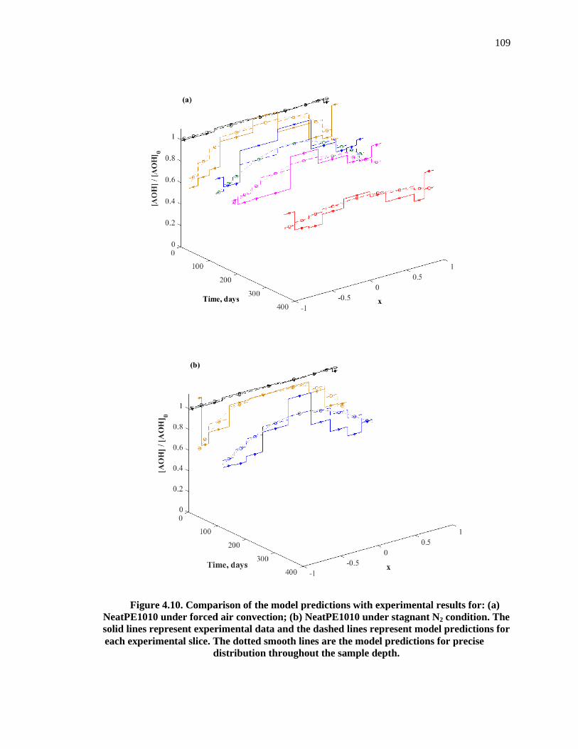
Figure 4.10. Comparison NeatPE1010 under forced air convection; (b) NeatPE1010 under stagnant Nsolid lines represent experimental data and the dashed lines represent model predictions for each experimental slice. The dotted smooth lines are the model predictions for precise

distribution throughout the sample depth.

. Comparison of the model predictions with experimental results for: (a) NeatPE1010 under forced air convection; (b) NeatPE1010 under stagnant Nsolid lines represent experimental data and the dashed lines represent model predictions for each experimental slice. The dotted smooth lines are the model predictions for precise

distribution throughout the sample depth.

109

of the model predictions with experimental results for: (a)

NeatPE1010 under forced air convection; (b) NeatPE1010 under stagnant N2 condition. The solid lines represent experimental data and the dashed lines represent model predictions for each experimental slice. The dotted smooth lines are the model predictions for precise

110

4.4.2 Table-Top Profile Observed for Irganox-1010

Table-top profiles of ‘Comp. 1010’ under forced-air conditions are shown in Figure 4.11(a).

The ‘table-top’ profile represents a typical AO concentration profile obtained for aged PE-clay

nanocomposites that has a flat AO-rich zone in the middle and AO-depleted surface regions.

These are compared with model predictions obtained using the reaction network of Figure 3.1(b)

and surface evaporation of ��. The initial free radical concentration is uniform which

eventually leads to uniform depletion of �� in the core region. Regeneration of � · is

necessary to continually deplete ��. This was brought about by degradation of ��. The rate

of �� degradation was adjusted to predict the experimental depletion rate as has been

discussed in Chapter 3, section 3.6.2. Figure 4.12 shows the average �� depletion and ��

depletion at the sample core at x=0 as functions of time (lines with circular marks). In Figure

4.12(a) the core AO obtained by the model approximately depletes exponentially, which is

similar to the experimental results as shown in Figure 4.12(b). Figure 4.12 also depicts the depth

of an AO-depleted layer penetrating towards the core as time progresses (lines with triangular and

square markers). The location of the edge of the AO-depleted layer is defined as the location

where ���� s 0.1. The growth trend of AO-depleted layer obtained by the model is similar to

the experimental results.

Figure 4.11. ComparisonComp.1010 under forced air condition; (b) Comp.1010 under slow air convection; (c)

Comp.1010 under stagnant Nthe dashed lines represent model predictions for each experimental slice. The dotted smooth lines are the model predictions for precise

. Comparison of the model predictions with experimental results for: (a) Comp.1010 under forced air condition; (b) Comp.1010 under slow air convection; (c)

Comp.1010 under stagnant N2 condition. The solid lines represent experimental data and t model predictions for each experimental slice. The dotted smooth

lines are the model predictions for precise distribution throughout the sample depth.

111

of the model predictions with experimental results for: (a) Comp.1010 under forced air condition; (b) Comp.1010 under slow air convection; (c)

condition. The solid lines represent experimental data and t model predictions for each experimental slice. The dotted smooth

distribution throughout the sample depth.

112

Figure 4.12. Depletion of total AO content and growth of depth of AO depleted layer with time for ‘Comp. 1010’ under forced-air condition: (a) Predictions by Model, (b)

Experimental observations.

Under the base-case model in section 4.3, Comp.1010 degradation and stabilization

mechanism was explained. Here, the model predicts that O2 reacts with all � · that were initially

present and then uniformly distributes throughout the sample after a few days of aging. The

resultant peroxide radical, � ·, is then stabilized by �� to generate hydroperoxide, ��.

The hydroperoxide decomposes fast due to catalytic action of clay and generates � · and � ·. � · is stabilized by �� and � · is oxidized again to continue the degradation reactions in a

cyclic manner. Until about 1020 days of aging �� is functional in protecting the polymer by

deactivating � · and � · free radicals as soon as they are generated by decomposition of

��. After 1020 days, the functional �� is completely depleted the polymer is no longer

protected from degradation. Complete �� depletion begins from surface due to a low ���� at

surface.

The difference in core AO and total AO depletion in Figure 4.12 is due to the additional loss

of AO from skin regions of sample. The reaction mechanism explains the overall accelerated AO

depletion in Comp1010 compared to neat PE. But to explain the skin AO depletion, some

additional mechanism like is high surface evaporation required. Also, in order to predict ‘table

top’ like AO profile, in addition to the surface depletion diffusion of AO also has to be low.

0 50 100 150 200 250 300 350 400 4500

0.1

0.2

0.3

0.4

0.5

0.6

0.7

0.8

0.9

1

[AO

H]/[

AO

H]

0

0 50 100 150 200 250 300 350 400 4500

0.1

0.2

0.3

0.4

0.5

0.6

0.7

0.8

0.9

1

Time, days

X*

(Dep

th o

f A

O d

eple

ted

laye

r fr

om s

urf

ace)

Model Predictions

[AOH]/[AOH] 0 < 0.1

(a)

Core [AOH]/[AOH]0

Avg [AOH]/[AOH] 0

0 50 100 150 200 250 300 350 400 4500

0.1

0.2

0.3

0.4

0.5

0.6

0.7

0.8

0.9

1

OIT

/OIT

0

0 50 100 150 200 250 300 350 400 4500

0.1

0.2

0.3

0.4

0.5

0.6

0.7

0.8

0.9

1

Time, days

X*

(Dep

th o

f A

O d

eple

ted

laye

r fr

om s

urfa

ce)

Experimental

OIT/OIT0 < 0.1

(b)

Avg OIT/OIT0

Core OIT/OIT0

113

To predict the sharp depletion of AO in ‘surface zone’ of ‘Comp. 1010’, the model considers

fast surface AO evaporation. Faster evaporation takes place under the condition of high air-

convection experienced during aging. To predict a ‘table-top’ like AO profile, the surface

evaporation loss has to be 100 times faster than neat PE and is therefore questionable.

In order to investigate whether this surface depletion is due to physical loss or due to

oxidative degradation, our collaborators conducted thermal aging of a similar Comp.1010 sample

under stagnant-N2 atmosphere. Under stagnant N2 condition, the sample was placed in a closed

cell with no convection. Figure 4.11(c) shows the AO profiles in obtained under such condition.

To predict the experimental results, oxygen concentration is assumed to be zero in the model and

the loss of AO was therefore only predicted by surface evaporation. The rate of evaporation of

AO, �¨©�, had to be reduced by 25 times in the model to predict AO evaporation at surface under

the N2 condition. Therefore, the evaporation rate of AO from Comp1010 surface under stagnant

N2 can be 4 times that of neat PE under high air convection. So, this indicates that the rate of AO

evaporation in Comp.1010 can be higher than neat PE under similar conditions of air convection.

A similar experiment was also conducted under ‘low air convection’ condition whose results

are shown in Figure 4.11(b). Here, the sample was placed in an open-top cell allowing a low air-

convection around the sample. The experimental results show that the surface AO depletion in

this case is faster than stagnant-N2 condition but slower than forced-air condition. A 10 times

reduction in �¨©� was required by the model to predict the AO depletion at surface. Hence, the

air-convection plays very important role in determining rate of surface depletion of AO.

Although the model predicts severe AO depletion at the very edge of sample surfaces in

Figure 4.11(a), the experimental results exhibit a thicker AO depleted skin layer especially during

first 200 days of aging. Figure 4.12(b) also shows that the depth of AO depleted layer during first

200 days of aging is higher than predicted by the model in Figure 4.12(a). Therefore, there could

114

be other factors besides evaporation that are responsible for this skin AO depletion and will be

discussed in section 4.5.

The AO depletion at the surface zone is brought about by the surface depletion together with

slow AO diffusion towards the surface. AO diffusion tends to smooth out the AO profile as in

case of NeatPE1010 giving it a parabolic shape. So, in order to predict a table-top profile lower

diffusivity is necessary, in which the depleted surface zone is not significantly replenished by AO

diffusing from core zone. A slower diffusion rate in Comp.1010 can be explained by tortuous

diffusive path of AO molecules caused by the clay platelets. In order to obtain good agreement

with experimental data, the AO diffusivity was reduced by 50% of ‘NeatPE1010’ as listed in

Table 4.2.

4.4.3 No Depletion in ‘NeatPE1076’

In ‘NeatPE1076’ under forced-air conditions experimental depletion of �� is negligible as

shown in Figure 4.13. Blooming is not expected because the solubility for Irganox-1076 in PE is

much higher (about 100 times) than the initial Irganox-1076 concentration shown in Table 2.3.

The model predicts that Irganox-1076 does not deplete due to negligible concentration of initial

free radicals which is stabilized by a small amount of ��, which is about 0.2% of its original

amount. The stabilization of oxidized free radicals produces hydroperoxides whose

decomposition is almost negligible. Slow surface depletion was achieved by limiting the

evaporation loss of �� through surface.

AO depletion due to reaction in both ‘NeatPE1010’ and ‘NeatPE1076’ are quite similar, and

are modeled using same reaction parameters. Both have negligible �� depletion by reaction.

‘NeatPE1010’ has a greater physical loss of AO due to blooming. The model considers the rate of

evaporation in ‘NeatPE1076’ to be larger than in ‘NeatPE1010’ to predict surface ��

concentration. This is justified because Irganox-1076 is more volatile at 85 °C than Irganox-1010.

In fact, at 85 °C Irganox-1076 is a liquid at sample surface while Irganox-1010 is a solid (Table

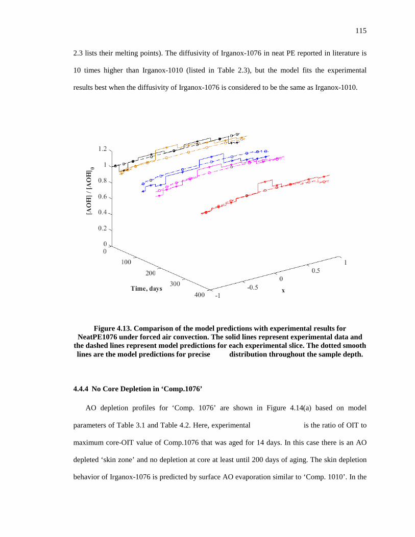
2.3 lists their melting points

10 times higher than Irganox

results best when the diffusi

Figure 4.13. Comparison of the model predictions with experimental results for NeatPE1076 under forced air convection. The solid lines represent experimental data and

the dashed lines represent model predictions for each experimental slice. The dotted smooth lines are the model predictions for precise

4.4.4 No Core Depletion in ‘Comp.1076’

AO depletion profiles for ‘Comp. 1076’ are shown in

parameters of Table 3.1 and

maximum core-OIT value of Comp

depleted ‘skin zone’ and no depletion at core

behavior of Irganox-1076 is

lting points). The diffusivity of Irganox-1076 in neat PE reported in literature

10 times higher than Irganox-1010 (listed in Table 2.3), but the model fits

he diffusivity of Irganox-1076 is considered to be the same as Irganox

. Comparison of the model predictions with experimental results for forced air convection. The solid lines represent experimental data and

the dashed lines represent model predictions for each experimental slice. The dotted smooth lines are the model predictions for precise distribution throughout the sample depth.

No Core Depletion in ‘Comp.1076’

profiles for ‘Comp. 1076’ are shown in Figure 4.14(a)

and Table 4.2. Here, experimental is the ratio of OIT to

OIT value of Comp.1076 that was aged for 14 days. In this case there is an AO

zone’ and no depletion at core at least until 200 days of aging. The s

1076 is predicted by surface AO evaporation similar to ‘Comp. 1010’

115

1076 in neat PE reported in literature is

, but the model fits the experimental

as Irganox-1010.

. Comparison of the model predictions with experimental results for forced air convection. The solid lines represent experimental data and

the dashed lines represent model predictions for each experimental slice. The dotted smooth distribution throughout the sample depth.

(a) based on model

is the ratio of OIT to

In this case there is an AO

. The skin depletion

oration similar to ‘Comp. 1010’. In the

116

model no AO depletion in ‘core zone’ is achieved by higher reactivity of the phenoxyl radical of

Irganox-1076 in terminating the oxidized free radicals (�·, and �·) that causes slow ��

depletion as discussed in Chapter 3, section 3.7.4. Therefore, in the model surface evaporation is

the main reason for AO depletion in this case. This surface evaporation has to be with same rate

(�¨©�) as in Comp.1010 in order to predict the severe surface AO depletion. Similar to the case of

Comp.1010, a high evaporation condition depletes AO only at the surface boundary which does

not predict the experiential thick AO depleted skin layer. Therefore this indicates that some other

factors are responsible for this AO depleted region that grows over time. Several potential factors

that can cause skin AO depletion will be discussed and evaluated in section 4.5.

The total OIT and core OIT are plotted against time progression as appears in Figure 4.15(a).

Experimental core-OIT in the sample core increases during first 2 months of aging and then starts

to decrease. This can be due to adsorption of AO molecules in clay and then its subsequent

desorption. If original OIT of ‘Neat PE 1076’ and ‘Comp. 1076’ are compared, it is observed that

there is a drop from 23 min to 16 min. This drop can be attributed to the adsorption of AO.

Besides this initial increase in �� concentration, the model predictions in Figure 4.15(a) are

qualitatively in good agreement with experimental observations.

Figure 4.14. Comparison of the model predictions with experimental results for: (a) Comp1076 under forced air convection; (b)

solid lines represent experimental data and the dashed lines represeach experimental slice. The dotted smooth lines are the model predictions for precise

distribution throughout the sample depth.

. Comparison of the model predictions with experimental results for: (a) under forced air convection; (b) Comp1076 under stagnant N

solid lines represent experimental data and the dashed lines represent model predictions for each experimental slice. The dotted smooth lines are the model predictions for precise

distribution throughout the sample depth.

117

. Comparison of the model predictions with experimental results for: (a)

N2 condition. The ent model predictions for

each experimental slice. The dotted smooth lines are the model predictions for precise

118

Figure 4.14(b) shows experimental �� depletion in Comp1076 under stagnant N2

atmosphere. The model considers a 10 times reduced evaporation rate to predict the experimental

surface depletion. When compared to Comp1010 under N2 atmosphere of Figure 4.11(b), here the

evaporation rate is 2.5 times faster which can be attributed to higher volatility of Irganox-1076.

Table 2.3 lists vapor pressure of Irganox-1076 to be much higher than Irganox-1010 at 25°C and,

therefore, justifies the higher volatility.

Figure 4.15. Depletion of total AO content and growth of depth of AO depleted layer with

time for ‘Comp. 1076’ under forced-air condition: (a) Predictions by Model, (b) Experimental observations.

4.5 Potential Causes of Antioxidant Depleted Skin Layer

The experimental OIT profiles in the aged PE-clay nanocomposites in Figure 4.11(a) and

Figure 4.14(a) show a skin layer devoid of AO after 30 days of aging whose depth increases with

aging time. In order to predict this experimental AO depleted skin, the model considered

evaporation of AO from the surface and diffusion-limited replenishment of AO to the skin.

However, to obtain a good model-experimental fit, the rate of AO evaporation (in Figure 4.11(a)

and Figure 4.14(a)) had to be increased 100 times more than the rate of evaporation used for pure

PE (of Figure 4.13). There is not a good justification for 100 times higher evaporation rate in

nanocomposites than in neat PE, end even with such a high evaporation, the model does not

0 100 200 300 4000

0.2

0.4

0.6

0.8

1

[AO

H]

/ [A

OH

] 0

0 100 200 300 4000

0.2

0.4

0.6

0.8

1

Time, days

X*

(Dep

th o

f A

O d

eple

ted

laye

r fr

om

sur

face

)

Model Predictions

(a)

[AOH]/[AOH] 0 < 0.5

Core [AOH]/[AOH]0Avg [AOH]/[AOH] 0

0 100 200 300 4000

0.2

0.4

0.6

0.8

1

OIT

/ O

IT0

0 100 200 300 4000

0.2

0.4

0.6

0.8

1

Time, days

X*

(Dep

th o

f A

O d

eple

ted

laye

r fr

om s

urfa

ce)

Experimental

(b)

OIT/OIT0 < 0.5

Core OIT/OIT0

Avg OIT/OIT0

119

predict the growth of the thickness of the depleted layer. In addition, Figure 4.11(b) shows that

the growth of the depleted layer is slower in experiments with slow air convection. An

explanation is that high evaporation under circulated air depletes AO from a very thin skin layer

which triggers some mechanism in the nanocomposites (but not in neat PE) causing this depleted

layer to grow. Therefore, the effect of evaporation cannot be entirely ignored. Cheng et al[21]

conducted an experiment to find the role of highly oriented clay at skin in depleting AO. When

the clay oriented skin layer was removed at the edges of samples prior to aging, they observed

reduced AO depletion at the surfaces. Therefore, the mechanism of skin formation appears to be

related to the presence of a layer of oriented clay particles.

The following section discusses the comparison between the model of this thesis and Cheng’s

experimental results for the AO depletion after removing the skin layer from the edge of a

specimen. Then there are several sections exploring alternative mechanisms for predicting the

rapid AO depletion in the skin layer: reduction in diffusivity of O2 and AO due to highly oriented

clay in the skin; higher oxidation rate in the skin; higher concentration of alkyl groups in the skin;

higher rate of �� decomposition in the skin; higher concentration of initial free radicals in the

skin; and additional generation of free radicals in the skin.

4.5.1 Effect of Clay Oriented Skin on rate of AO Depletion

Cheng et al.[21] conducted an experimental investigation on the effect of highly oriented clay

layer on the rate of AO depletion at skin layer of Comp.1010 samples. The sample preparations

are shown in Figure 4.16. Figure 4.16(a) shows the whole injection molded Comp.1010 sample

which was subjected to aging at 85°C under forced air, whereas Figure 4.16(b) shows a

Comp.1010 sample with the highly clay oriented edges removed prior to aging. Although the

slicing method for determining OIT profile is different than those discussed earlier in this chapter

(Figure 1.3(b)), both techniques gives approximately similar results. This is because the skin layer

120

from top and bottom (represented by grayish slices) are removed from the slices before

conducting the OIT tests.

Figure 4.16. Schematic diagrams of Comp.1010 samples showing the technique used to

measure: (a) OIT profiles through sample depth from clay oriented surface to interior of the samples; and (b) OIT profiles from surface to core for samples with skin layers removed

before aging process. [21]

Figure 4.17 shows the experimental AO depletion profiles for Comp.1010 with and without

the skin layer that are aged for 120 days at 85°C under circulated air. The model predictions are

also shown in the figure in dashed-lines. The experimental result in Figure 4.17(a) after 120 days

of aging shows an AO depleted layer of about 0.16 scaled depth which is not predicted by the

base-case model. The experimental AO depletion profile for x < 0.16 follows a trend similar to

the model prediction. With the clay oriented skin layer removed prior to aging, Figure 4.17(b)

shows AO to be only partially depleted from the new un-oriented skin layer which is attributed to

surface evaporation. For the model to reproduce these experimental results, the value of �¨© � �

is 5 times that of the neat PE in order to predict the experimental skin AO depletion. In this case,

the evaporation coefficient is used as an adjustable parameter to fit the depletion in the skin layer;

there is not a clear rationale for why the evaporation coefficient would be 100 times more than

neat PE when there is an oriented clay layer and 5 times more when the oriented clay layer has

been removed. Therefore, the following sections explore several mechanisms, besides the

evaporation, to predict the observed depletion in the skin layer. The main morphological

(b) (a)

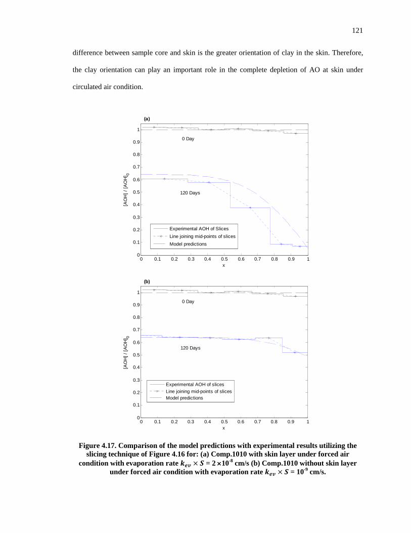
121

difference between sample core and skin is the greater orientation of clay in the skin. Therefore,

the clay orientation can play an important role in the complete depletion of AO at skin under

circulated air condition.

Figure 4.17. Comparison of the model predictions with experimental results utilizing the slicing technique of Figure 4.16 for: (a) Comp.1010 with skin layer under forced air

condition with evaporation rate ²�³ � � = 2 ××××10-8 cm/s (b) Comp.1010 without skin layer under forced air condition with evaporation rate ²�³ � � = 10-9 cm/s.

0 0.1 0.2 0.3 0.4 0.5 0.6 0.7 0.8 0.9 10

0.1

0.2

0.3

0.4

0.5

0.6

0.7

0.8

0.9

1

x

[AO

H]

/ [A

OH

] 0

Experimental AOH of Slices

Line joining mid-points of slices

Model predictions

120 Days

0 Day

(a)

0 0.1 0.2 0.3 0.4 0.5 0.6 0.7 0.8 0.9 10

0.1

0.2

0.3

0.4

0.5

0.6

0.7

0.8

0.9

1

x

[AO

H]

/ [A

OH

] 0

Experimental AOH of slices

Line joining mid-points of slicesModel predictions

0 Day

120 Days

(b)

122

4.5.2 Variable Diffusivity of O 2 and AO

It has been discussed by Cheng et al.[21] that the highly oriented clay at the nanocomposite

skin offers an increased tortuous diffusion path for AO and O2. This causes slower diffusion of

AO and O2 in the skin layer of the nanocomposites whose depth is expected to be around a scaled

value of x = 0.7 corresponding to the depths AO depleted layer in Comp.1010 and Comp.1076.

Several researchers have proposed equations to estimate the diffusivities as function of degree of

clay orientations. For example, Bharadwaj[8] proposed the following model to estimate

diffusivities in polymer composites, which correlates between clay length (�), volume fraction

(´µ), relative orientation (�¶), and thickness (�).

£µ£ ·¯ �µ� ¸ g 1 J ´µ1 - �2� ´µ x23y x�¶ - 12y 4.15

Where, £µ and £ are the permeabilities of mobile molecules in of PE-Clay nanocomposites and

neat PE, respectively. �µ and � are the diffusivities of mobile molecules in PE-Clay

nanocomposites and neat PE, respectively. The composition of nanocomposites in units of

percent weight is given in Table 3.4. With density of PE, ¹º»=0.939 g/cm3 and density of the

modified clay, ¹µ=1.7 g/cm3, the volume fraction of clay, ́µ, is found to be 0.0225. The required

properties of clay are tabulated in Table 4.3 where the length and width of clay are measured

from TEM images of the nanocomposites provided by collaborators on this research.

Table 4.3. Various parameters of clay

Parameters Values

� 85 nm - 242 nm

� 4 nm - 37 nm

¹µ 1.7 g/cm3

´µ 0.0225

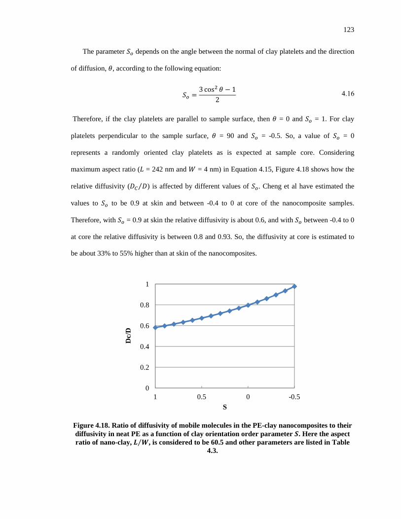
123

The parameter �¶ depends on the angle between the normal of clay platelets and the direction

of diffusion, ¼, according to the following equation:

�¶ g 3 cos ¼ J 12 4.16

Therefore, if the clay platelets are parallel to sample surface, then ¼ = 0 and �¶ = 1. For clay

platelets perpendicular to the sample surface, ¼ = 90 and �¶ = -0.5. So, a value of �¶ = 0

represents a randomly oriented clay platelets as is expected at sample core. Considering

maximum aspect ratio (� = 242 nm and � = 4 nm) in Equation 4.15, Figure 4.18 shows how the

relative diffusivity (�µ �⁄ ) is affected by different values of �¶. Cheng et al have estimated the

values to �¶ to be 0.9 at skin and between -0.4 to 0 at core of the nanocomposite samples.

Therefore, with �¶ = 0.9 at skin the relative diffusivity is about 0.6, and with �¶ between -0.4 to 0

at core the relative diffusivity is between 0.8 and 0.93. So, the diffusivity at core is estimated to

be about 33% to 55% higher than at skin of the nanocomposites.

Figure 4.18. Ratio of diffusivity of mobile molecules in the PE-clay nanocomposites to their diffusivity in neat PE as a function of clay orientation order parameter �. Here the aspect ratio of nano-clay, ½ ¾⁄ , is considered to be 60.5 and other parameters are listed in Table

4.3.

0

0.2

0.4

0.6

0.8

1

-0.500.51

Dc/

D

S

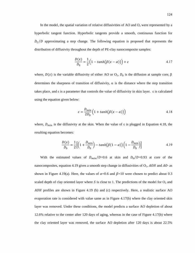
124

In the model, the spatial variation of relative diffusivities of AO and O2 were represented by a

hyperbolic tangent function. Hyperbolic tangents provide a smooth, continuous function for

�µ �⁄ approximating a step change. The following equation is proposed that represents the

distribution of diffusivity throughout the depth of PE-clay nanocomposite samples:

�]!^�� g 1

2 x1 J fp¿Àu�]! J �^vy - Á 4.17

where, �]!^ is the variable diffusivity of either AO or O2, �� is the diffusion at sample core, β

determines the sharpness of transition of diffusivity, α is the distance where the step transition

takes place, and ε is a parameter that controls the value of diffusivity in skin layer. ε is calculated

using the equation given below:

Á g ��� 2�� x1 - fp¿Àu�]! J �^vy 4.18

where, ��� is the diffusivity at the skin. When the value of ε is plugged in Equation 4.18, the

resulting equation becomes:

�]!^�� g 1

2 ·1 - ��� �� ¸ J fp¿Àu�]1 J �^v ·1 J ��� �� ¸Ã 4.19

With the estimated values of ��� �⁄ =0.6 at skin and �� �⁄ =0.93 at core of the

nanocomposites, equation 4.19 gives a smooth step change in diffusivities of O2, �� and �· as

shown in Figure 4.19(a). Here, the values of �=0.6 and �=10 were chosen to predict about 0.3

scaled depth of clay oriented layer where � is close to 1. The predictions of the model for O2 and

�� profiles are shown in Figure 4.19 (b) and (c) respectively. Here, a realistic surface AO

evaporation rate is considered with value same as in Figure 4.17(b) where the clay oriented skin

layer was removed. Under these conditions, the model predicts a surface AO depletion of about

12.6% relative to the center after 120 days of aging, whereas in the case of Figure 4.17(b) where

the clay oriented layer was removed, the surface AO depletion after 120 days is about 22.5%

125

relative to the center. The experimental OIT of the skin slice is about 18.5 times lower than the

OIT at sample center. The surface AO depletion in the case of Figure 4.19(c) is less because of

lower diffusion of AO from interior of samples to the surface. When compared to Figure 4.11(a),

the AO depleted skin layer formed in 30 days of aging is not predicted by the gradient in

diffusivity.

Figure 4.19. Distribution of: (a) diffusivity; (b) oxygen; and (c) phenolic groups in AO

throughout the depth of Comp.1010 under the conditions of hyperbolic tangent distribution of diffusion in Equation 4.19 and evaporation rate 5 times more than NeatPE1076 (²�³ � �

= 10-9 cm/s). Here Ä=0.6, Å=10, ÆÇ�� Æ⁄ =0.6 and Æj Æ⁄ =0.93.

When the diffusivity at skin was reduced by factors of 100 and 1000 times that of core in

Figure 4.20 and Figure 4.21 respectively, it is observed that the low diffusivity on the skin layer is

a bottleneck to the flux of O2 from the surface into the core causing a high O2 concentration at

skin layer compared to core. A high [O2] in the skin together with slow replenishment of ��

from the nanocomposite core causes faster depletion of �� on the skin. But even with such

exaggerated non-homogeneity in diffusion, the model is unable to predict a completely AO

depleted skin after 30 days of aging.

In order to predict a ‘table top’ AO profile, the model has to consider about 1000 times

reduced diffusivity at skin than at core. This causes a boundary layer in [O2] as in Figure 4.21(b)

due to slow penetration through skin and rapid reaction. This rapid oxidation on the skin causes

0 0.5 10

0.2

0.4

0.6

0.8

1

x

D(x

) /

D

0 0.5 10

0.2

0.4

0.6

0.8

1

x

[O2]

/ [O

2] sat

0 0.5 10

0.2

0.4

0.6

0.8

1

x

[AO

H]

/ [A

OH

] 0

30 days

60 days

90 days

445 days(a) (b) (c)

126

AO to deplete. But low [O2] at core causes slow depletion of AO from sample core. Increasing

the rate of catalytic hydroperoxide decomposition, ��� , does not increase the AO depletion any

further because for ��� > 105 cm3/mol-s, the �� decomposition reaction is no longer the rate

limiting step. So, in order to predict the experimental core AO depletion, a high [O2] is required at

the core. Therefore, both core and skin AO depletion could not be predicted at one time by

utilizing the non-homogeneous distribution of diffusivity.

Figure 4.20. Distribution of: (a) diffusivity; (b) oxygen; and (c) phenolic groups in AO

throughout the depth of Comp.1010 under the conditions of Figure 4.19 with diffusivity at skin 100 times lower than at core.

Figure 4.21. Distribution of: (a) diffusivity; (b) oxygen; and (c) phenolic groups in AO

throughout the depth of Comp.1010 under the conditions of Figure 4.19 with diffusivity at skin 1000 times lower than at core.

0 0.5 10

0.2

0.4

0.6

0.8

1

x

D(x

) /

D

0 0.5 10

0.2

0.4

0.6

0.8

1

x

[O2]

/ [O

2] sat

0 0.5 10

0.2

0.4

0.6

0.8

1

x[A

OH

] /

[AO

H] 0

(a) (b) (c)

60 days

90 days

445 days

445 days

30 days

30 days

0 day

0 0.2 0.4 0.6 0.8 10

0.1

0.2

0.3

0.4

0.5

0.6

0.7

0.8

0.9

1

x

D(x

) /

D

0 0.2 0.4 0.6 0.8 10

0.1

0.2

0.3

0.4

0.5

0.6

0.7

0.8

0.9

1

x

[O2]

/ [O

2] sat

0 0.2 0.4 0.6 0.8 10

0.1

0.2

0.3

0.4

0.5

0.6

0.7

0.8

0.9

1

x

[AO

H]

/ [A

OH

] 0

(a) (b) (c)

445 days

30 days

127

4.5.3 Non-uniform oxidation rate constant, ²�

During the thermal aging process the average flux of O2 is perpendicular to the sample

surface because O2 diffuses from sample surface towards sample core. The oriented clay particles

in the sample skin layer create a more tortuous path because O2 needs to pass around clay flakes.

This may enhance the oxidation rate of free radicals in the skin.

To accommodate this hypothesis, the oxidation rate in the skin layer is considered to be

higher than at the core. In the base-case model, the value of k1 was modified by a step change

with 109 cm3/mol-s in the core (x < 0.7) and 1010 cm3/mol-s in the skin region (x > 0.7). The

model prediction with the modified step change in k1 and evaporation rate constant 5 times more

than NeatPE1076 (�¨© � � = 10-9 cm/s) are shown in Figure 4.22. In Figure 4.22(c), the ���� profile shows a greater depletion at skin by about 30% relative to center. But when this depletion

is compared with ���� depletion with uniform �� shown in Figure 4.23(b), the skin depletion is

almost the same. Even with a greater step change of 100 times higher oxidation constant at skin in

Figure 4.23(a), the ���� depletion is 28% relative to center. Therefore, the variation in the

oxidation rate constant has negligible contribution in skin AO depletion. This is because in the

nanocomposite degradation reaction network of Figure 3.1(b), the overall rate limiting step is the

�� decomposition. So, increasing the value of �� does not increase the rate of oxidation. But

if instead of increased oxidation constant at skin, the oxidation constant at core is decreased, then

the oxidation reaction at core can become rate limiting as shown in Figure 4.23(c). Although in

this figure, the skin ���� is about 38.5% lower the core, the reduced oxidation at core reduces

the core AO depletion and no longer matches the experimental AO depletion. Also, even under

such condition, the model is not able to predict complete skin AO depletion after 30 days of

aging.

128

Therefore, a greater oxidation rate constant at the nanocomposite skin does not predict

additional AO depletion at skin as long as the actual oxidation rate is limited by hydroperoxide

decomposition rate.

Figure 4.22. Distribution of: (a) oxidation constant; (b) oxygen; and (c) phenolic groups in

AO throughout the depth of Comp.1010 under the conditions of the base-case with modified �� and evaporation rate of ²�³ � � = 10-9 cm/s.

Figure 4.23. Distribution of phenolic groups in AO throughout the depth of Comp.1010

under the conditions of Figure 4.22 with: (a) ��(skin) = 100 ×××× ��(core), (b) uniform ��, and (c) ��(core) = 0.1 ×××× ��(skin).

4.5.4 Non-Uniform distribution of alkyl groups capable of donating hydrogen, �i&�j

In Chapter 3, section 3.3, it is discussed that ���� is the concentration of sites in PE from

which free radicals can abstract hydrogen. It was also discussed that the free radicals can abstract

0 0.5 10

2

4

6

8

10

x

k 1 / k

1(cor

e)

0 0.5 10

0.2

0.4

0.6

0.8

1

x

[O2]

/ [O

2] sat

0 0.5 10

0.2

0.4

0.6

0.8

1

x

[AO

H]

/ [A

OH

] 0

0 day(a) (b) (c)

Core

30 days andabove

450 days

Skin

30 days

0 0.2 0.4 0.6 0.8 10

0.2

0.4

0.6

0.8

1

x

[AO

H]

/ [A

OH

] 0

0 0.2 0.4 0.6 0.8 10

0.2

0.4

0.6

0.8

1

x

[AO

H]

/ [A

OH

] 0

0 0.2 0.4 0.6 0.8 10

0.2

0.4

0.6

0.8

1

x

[AO

H]

/ [A

OH

] 0

(c)(b)(a)445 days

30 days

445 days

30 days

445 days

30 days

k1(skin)=109 cm3/mol-s

k1(core)=108 cm3/mol-s

k1(skin)=109 cm3/mol-s

k1(core)=109 cm3/mol-s

k1(skin)=1011 cm3/mol-s

k1(core)=109 cm3/mol-s

129

hydrogen from almost any C, but the C-H dissociation energies of different hydrocarbon groups

in PE can have a wide spectrum. The dissociation energies depend on the position of C atom in

the order of: allyl < tertiary < secondary < primary. An analysis shown in Appendix B shows that

the H-abstraction rate from allyl, tertiary and secondary C-atoms can be higher than H-abstraction

rate from primary C-atom by about 100 times, 16 times and 4 times respectively. Therefore, the

variation in rate constants of H-abstraction can vary by two orders of magnitude. Although such

variation exists, usually in the models reported in literature (including this dissertation) all these

different C-H structures are assumed to be represented by a single variable, ��, and is often even

considered to be a constant. Also, during PE degradation there can be different rates of generation

of different types of C-H structure. Therefore, the assumptions can be challenged. In order to

predict PE degradation with better accuracy, each type of C-H structure has to be considered as

separate variables.

It might be argued that with uniform initial distribution and uniform generation of these

different C-H structures, the assumption of single �� variable would be valid. But in case of non-

uniform distribution of these C-H structures, the �� decomposition rate would also become

non-uniform because it reacts with the �� groups. The non-uniform �� distribution can be

caused by high shear rate experienced by the PE molecules at the skin during sample molding. In

case of the nanocomposites, the orientated clay flakes at skin may enhance the shear rate. This

may cause PE molecular chain to break across a C-C bond. In absence of oxygen during molding,

this chain breakage can create unsaturated C=C bonds thereby increasing the concentration of

allylic C atoms that increases ���� at the skin region.

Figure 4.24 and Figure 4.25 shows the predicted concentration profiles of various species

made by the base-case model when the ����� is modified by a step change with 10-4 mol/cm3 in

the core (x < 0.7) and 10-3 mol/cm3 in the skin region (x > 0.7) and with evaporation rate constant

�¨© � � = 10-9 cm/s. Figure 4.24(c) shows a drastic depletion of ���� at the skin. This is

130

because of greater �� decomposition rate due to higher ���� which makes the reaction cycle

of Figure 3.1(b) faster. In Figure 4.25, the abrupt rise in concentrations of various species in the

core-skin junction is due to sudden increase in ���� caused by the initial step change.

In Figure 4.24(c), the shoulder of the ‘table top’ ���� profile is predicted to move inwards

with aging time following a similar trend as predicted by the base-case model in Figure 4.2(b)

that considered excessively high surface AO evaporation rate. Although a higher depletion of AO

is predicted, but it does not completely deplete AO at the skin at 30 days of aging. Figure 4.26

and Figure 4.27 shows the distribution of O2 and AO with skin ����� 15 times and 5 times

respectively greater than at core. In Figure 4.26(c) an increased step size shows a greater degree

of skin AO depletion after 30 days when compared to Figure 4.24(c).

With the step change at ! > 0.7 in the model, the thickness of AO depleted skin layer appears

to be large at 30 days of aging when compared with experimental results. Therefore, in order to

predict the experimental results, a higher ����� is required to completely deplete AO within 30

days of aging at a very thin skin layer that grows with aging time.

Figure 4.24. Distribution of: (a) �����; (b) oxygen; and (c) phenolic groups in AO throughout the depth of Comp.1010 under the conditions of the base-case with modified

����� and evaporation rate of ²�³ � � = 10-9 cm/s.

0 0.5 10

2

4

6

8

10

x

[RH

] 0 / [

RH

] 0(cor

e)

0 0.5 10

0.2

0.4

0.6

0.8

1

x

[O2]

/ [O

2] sat

0 0.5 10

0.2

0.4

0.6

0.8

1

x

[AO

H]

/ [A

OH

] 0

(a) (b) (c)

CoreSkin

445 days

30 daysand above

Decreaseafter 360days

30 days

360 days

0 day

0 day

131

Figure 4.25. Concentration profiles of various polymeric species under the conditions of

Figure 4.24. Inset figures display the same data with magnified vertical axis.

Figure 4.26. Distribution of: (a) �i&�j; (b) oxygen; and (c) phenolic groups in AO

throughout the depth of Comp.1010 under the conditions of Figure 4.24 with �i&�j = 10-4 mol/cm3 at core in the core (x < 0.7) and �i&�j = 15 ×××× 10-3 mol/cm3 in the skin. In the middle

figure (b), the circled points and arrow shows the time progression of O2 profiles.

0 0.5 10

1

2

3x 10

-5

x

[R*]

/[R

*]0(c

ore)

0 0.5 10

2

4

6

8

10x 10

4

x

[RH

]/[R

*]0(c

ore)

0 0.5 10

2

4

6

8

x

[RO

O*]

/[R

*]0(c

ore)

0 0.5 10

200

400

600

800

x

[RO

OH

]/[R

*]0(c

ore)

0 0.5 10

2

4

6

8x 10

-3

x

[RO

*]/[

R*]

0(cor

e)

0 0.5 10

0.5

1

1.5

2

x

[AO

*]/[

R*]

0(cor

e)

0 0.5 10

2

4

x 10-6

0 0.5 10

0.5

1x 10

-5

0 0.5 10

1

2x 10

-7

0 0.5 10

5

10

15

(c)(b)

(d) (e) (f)

(a)

0 0.5 10

2

4

6

8

10

12

14

16

x

[RH

] 0 / [

RH

] 0(cor

e)

0 0.5 10

0.2

0.4

0.6

0.8

1

x

[O2]

/ [O

2] sat

0 0.5 10

0.2

0.4

0.6

0.8

1

x

[AO

H]

/ [A

OH

] 0

(a) (b) (c)

30 days

0 day

30 daysand above

Core

450 days

450 days

0 day

o

o

oo

ooo

o210 days

Skin

132

Figure 4.27. Distribution of: (a) �����; (b) oxygen; and (c) phenolic groups in AO throughout the depth of Comp.1010 under the conditions of Figure 4.24 with �i&�j = 10-4

mol/cm3 at core in the core (x < 0.7) and �i&�j = 15 ×××× 10-3 mol/cm3 in the skin.

4.5.5 Non-uniform i%%& decomposition rate constant, ²l, due to non-uniformity in the catalytic action of clay

Non-uniform catalytic action of clay can be due to variation in clay concentration or variation

in the interaction of the quarternary-ammonium ions with PE molecules through the depth of the

PE-clay nanocomposite samples. The variation in clay concentration can be the result of oriented

and disoriented clay regions and the variation in interaction of quarternary-ammonium ions can

be the result of variation in the degree of clay intercalation/exfoliation.

If the clay concentration is higher in the clay-oriented skin layer, the catalytic effect of clay in

this layer would be higher enhancing the hydroperoxide decomposition constant, ��. Similar ��

enhancement can occur if a higher shear rate at sample skin is experienced during sample

molding causing a greater exfoliation of clay galleries at skin exposing more quarternary

ammonium ions into PE matrix. To include this hypothesis of enhanced �� on the skin, the base-

case model is modified with value of ��� in the core considered to be 105 s-1 and for skin layer (x >

0.7) is considered to be 106 s-1. Figure 4.28 shows the results obtained using this modified base-

case with evaporation rate constant �¨© � � = 10-9 cm/s. In Figure 4.28(c), the AO depletion in

the skin region is only slightly increased. Further increasing the value of ��� in the skin does not

0 0.5 10

1

2

3

4

5

6

x

[RH

] 0 / [

RH

] 0(cor

e)

0 0.5 10

0.2

0.4

0.6

0.8

1

x

[O2]

/ [O

2] sat

0 0.5 10

0.2

0.4

0.6

0.8

1

x

[AO

H]

/ [A

OH

] 0

(a) (b) (c)

30 days

0 day

30 daysand above

Core

0 day

Skin

450 days

133

increase the AO depletion as well. This is because with increased value of ��� , the hydroperoxide

decomposition reaction is no longer rate determining for the overall degradation cycle. This

causes ���� to reduce to nearly zero at skin region and so increasing the value of ��� does not

increase its decomposition rate.

Figure 4.28. Distribution of: (a) i%%& decomposition constant; (b) oxygen; and (c) phenolic groups in AO throughout the depth of Comp.1010 under the conditions of base-

case with modified ²l� and evaporation rate of ²�³ � � = 10-9 cm/s.

4.5.6 Non-Uniform initial alkyl free radical concentratio n, �i·�j

A non-uniform initial free radical concentration, ��·��, can deplete more AO from the

nanocomposite skin compared to core if their concentration on the skin is higher. During the

initial transient reactions, the rate of oxidation at skin is higher due to higher ��·�� which causes

higher consumption of ��. The rate of oxidation at later stages depends on generation of �· by

�� decomposition cycle which has been shown to be unaffected by ��·�� in Chapter 3,

Section 3.8.6. Therefore, ��·�� can only affect the initial transient reactions. So, if initial ��·�� at

skin is comparable to ����� then, almost all �� at skin can be depleted.

Figure 4.29 and Figure 4.30 show distribution profiles of [O2] and ���� when non-uniform

values ��·�� are considered with a step change at ! = 0.7. The evaporation rate constant

considered is �¨© � � = 10-9 cm/s with the rest of the parameters are same as the base-case of

0 0.5 10

2

4

6

8

10

x

k' 3 / k

' 3(cor

e)

0 0.5 10

0.2

0.4

0.6

0.8

1

x

[O2](

x,t)

0 0.5 10

0.2

0.4

0.6

0.8

1

x

[AO

H]

/ [A

OH

] 0

0 day(a) (b) (c)

CoreSkin

30 days and above

445 days

30 days

134

Comp.1010. Figure 4.29(a) shows 10 times higher skin ��·�� than at core, which causes higher

depletion of �� at skin shown in Figure 4.29(c) but not high enough to predict the experimental

skin depletion. When the ��·�� at skin is increased to 600 times that at core (Figure 4.30) then

��·� becomes comparable to ����� and is able to completely deplete �� from the skin layer

as shown in Figure 4.30(c).

Figure 4.29. Distribution of: (a) alkyl free radical; (b) oxygen; and (c) phenoxyl groups in

AO throughout the depth of Comp.1010. Here the initial [i····] at skin is 10 time higher than at core.

Figure 4.30. Distribution of: (a) alkyl free radical; (b) oxygen; and (c) phenoxyl groups in AO throughout the depth of Comp.1010. Here the initial [i····] at skin is 600 times higher

than at core.

Therefore, in order to predict AO depleted skin layer, the ��·�� at skin has to be 600 times or

more than at core. Although, this assumption can predict depletion of skin AO, but the growth of

this layer is not predicted. Also, such a high degree of variation in ��·�� is questionable.

0 0.2 0.4 0.6 0.8 10

1

2

3

4

5

6

7

8

9

10

11

x

[R*]

0 / [

R*]

s

0 0.2 0.4 0.6 0.8 10

0.1

0.2

0.3

0.4

0.5

0.6

0.7

0.8

0.9

1

x

[O2]

/ [O

2] sat

0 0.2 0.4 0.6 0.8 10

0.1

0.2

0.3

0.4

0.5

0.6

0.7

0.8

0.9

1

x

[AO

H]

/ [A

OH

] 0

(a) (b) (c) 445 days

30 days30 days and above

0 day

CoreSkin

0 0.2 0.4 0.6 0.8 10

100

200

300

400

500

600

x

[R*]

0 / [

R*]

s

0 0.2 0.4 0.6 0.8 10

0.1

0.2

0.3

0.4

0.5

0.6

0.7

0.8

0.9

1

x

[O2]

/ [O

2] sat

0 0.2 0.4 0.6 0.8 10

0.1

0.2

0.3

0.4

0.5

0.6

0.7

0.8

0.9

1

x

[AO

H]

/ [A

OH

] 0

(a) (b) (c) 445 days

30 days30 days and above

0 day

CoreSkin

135

Therefore, the severe skin AO depletion has to be explained by some other mechanisms with

realistic parameters.

4.5.7 Additional generation of [i····] at PE-clay nanocomposite skin

The hydroperoxide decomposition mechanism is usually the main cause of polymer

degradation. But if under certain conditions the PE molecule is strained, it can give rise to

molecular defects. Such molecular defects can generate additional free radicals free radicals

thereby increasing the oxidative degradation rate.

During the molding process of PE-clay nanocomposites samples, the clay flakes and PE

molecules at skin are oriented along the direction of melt flow and experience a thermal quench.

The PE molecules in the interior of the sample take longer time to cool down and so get greater

opportunity to obtain stable conformations. The ordered PE molecules and clay in the skin can

therefore be strained at certain points. During the aging process, any such strained point can give

rise to C-C bond scission and the free radicals generated can be quickly oxidized to propagate

further degradation reactions. The degradation results in further C-C bond scission via reaction

R.6 in Table 2.1. Therefore, once a C-C bond breaks due to strain, the degradation reactions that

follow can cause more and more C-C bond scissions to eventually create a submicron-crack. The

degradation can become even more severe if these submicron-cracks induce additional stress and

strain and propagate by more and more C-C scission. Usually a formation of submicron crack is

accompanied by the rupture of about 100 – 1000 C-C bonds[22].

To accommodate this hypothesis in the model, an additional generation rate of alkyl free

radicals has been considered for the skin region. Assuming this generation to be constant over the

experimental time (~500 days), the equation 3.3 governing mass-balance across � · is modified by

the following equation in the skin layer (! > 0.7).

136

d�� ·�®È� df g Jk��� ·��O � - k �� ·����� - k��������� - kM�� ·�����- k��� ·� - k�������� ·� J k���� ·��� ·� - "#·

4.20

where "#· is the additional generation term. With a value of "#· g 10 � �� ·��o �⁄ = 3.9 × 10-14

cm3/mol-s and evaporation constant �¨© � � = 10-9 cm/s, the base-case model predicts various

concentration profiles as shown in Figure 4.31 and Figure 4.32. Here, �� ·��o �⁄ is the non-

dimensional scale of reaction rate used in the model whose value is 3.9 × 10-15 cm3/mol-s.

In Figure 4.31(b), [��] profiles show a greater degree of AO depletion in skin than at core.

A constant generation of �· maintains a high ����, �� ·� and �� ·� in the skin layer as

shown in Figure 4.32 (b), (e) and (f) respectively. This elevated concentration of the reactive

species causes sharp depletion of ���� in the skin.

Figure 4.31. Distribution of: (a) oxygen; and (b) phenolic groups in AO throughout the depth of Comp.1010 under the conditions of additional generation of i···· at É > 0.7 with �i· =

3.9××××10-14 cm3/mol-s in Equation 4.20 and surface AO evaporation rate of ²�³ � � = 10-9 cm/s.

0 0.5 10

0.2

0.4

0.6

0.8

1

x

[O2]

/ [O

2] sat

0 0.5 10

0.2

0.4

0.6

0.8

1

x

[AO

H]

/ [A

OH

] 0

Skin

Core

30 days and above 30 days

450 days

0 day(a) (b)

137

Figure 4.32. Concentration profiles of various polymeric species under the conditions of

Figure 4.31. Inset figures display the same data with magnified vertical axis.

It was observed that in order to predict a high AO depletion at skin, the value of "#· had to be

comparable to the � · consumption terms in equation 4.20. The �· consumption terms are

‘k��� ·��O �’ and ‘k���� ·��� ·�’ whose values are on the order of 10-13 cm3/mol-s and 10-15

cm3/mol-s respectively. Figure 4.33 (a) and (b) shows the AO depletion profile with "#· values 10

times lower and 10 times higher respectively than the value of "#· of Figure 4.31(c). With a "#· value lower than about 10-14 cm3/mol-s, the model is not able to predict complete skin AO

depletion even after 450 days of aging (Figure 4.33(a)).

With a high value of "#· in Figure 4.33(b), the shoulder of the ‘table top’ ���� profile is

predicted to move inwards with aging time following a similar trend as predicted by the base-case

model in Figure 4.2(b) and by non-uniform ����� model in Figure 4.24(c). With the step change

at ! > 0.7 in the model, the thickness of AO depleted skin layer appears to be large at 30 days of

0 0.5 10

1

2

3x 10

-7

x

[R*]

/[R

*]0

0 0.5 10

2000

4000

6000

8000

10000

x

[RH

]/[R

*]0

0 0.5 10

0.2

0.4

0.6

0.8

1

x

[RO

O*]

/[R

*]0

0 0.5 10

2

4

6

8

10

x

[RO

OH

]/[R

*]0

0 0.5 10

0.2

0.4

0.6

0.8

1x 10

-4

x

[RO

*]/[

R*]

0

0 0.5 10

0.5

1

1.5

x

[AO

*]/[

R*]

0

0 0.5 10

1

2x 10

-6

0 0.5 10

2

4

x 10-6

0 0.5 10

2

4

x 10-8

(b) (c)(a)

(d) (e) (f)

138

aging when compared with experimental results. Therefore, in order to predict the experimental

results, a high "#· is required to completely deplete AO within 30 days of aging at a very thin

skin layer that grows with aging time.

Figure 4.33. Distribution of phenolic groups in AO throughout the depth of Comp.1010 under the conditions of Figure 4.31 with (a) �i· = 3.9××××10-15 cm3/mol-s and (b) �i· = 3.9××××10-13

cm3/mol-s.

4.5.8 Summary of the potential causes of skin AO depletion

Several hypotheses explaining the severe depletion of AO from skin region have been

described in this section, the main features of which are summarized in Table 4.4. The hypotheses

of ‘non-uniform �����’ and ‘additional generation of � · at skin’ have the potential to predict

complete depletion of AO from the skin layer than can grow with time. But, there is no

experimental data to evaluate the parameters in both the cases. The hypotheses of ‘surface AO

evaporation’, ‘non-uniform diffusivity’ and ‘non-uniform �� ·�� can predict surface/skin AO

depletion with exaggerated values of the parameters, but the growth of depleted skin layer is not

predicted. The hypotheses of ‘non-uniform �· oxidation’ and ‘non-uniform ��

decomposition’ were not able to predict a depleted skin layer. Therefore, the ‘non-uniform

�����’ and ‘additional generation of � · at skin’ might be the causes of skin AO depletion both of

0 0.5 10

0.2

0.4

0.6

0.8

1

x

[AO

H]

/ [A

OH

] 0

0 0.5 10

0.2

0.4

0.6

0.8

1

x

[AO

H]

/ [A

OH

] 0

450 days(b)(a)

30 days30 days

450 days

139

which can be related to C-C scission in the skin caused by strained PE molecules. In addition to

these, the partial effects of ‘surface AO evaporation’ and ‘non-uniform diffusivity’ cannot be

totally ignored.

Table 4.4. Comparison of various hypotheses in depleting AO from skin region of PE-clay nanocomposites

Case Cause Parameters influenced Features

Surface AO evaporation

High air convection �¨©�

• Predicts surface AO depletion with exaggerated values

• Does not predict depth of skin layer that increases with time

Non-uniform Diffusivity

Highly oriented clay at skin

�� , �¦�«, �¦�· • Cannot predict both surface and

skin AO depletion simultaneously • Predicts surface AO depletion with

exaggerated values

Non-uniform � · oxidation rate

Higher residence time of O2 in skin �� • Does not predict skin AO depletion

Non-uniform �����

Higher conc. of weak C-H bonds

at skin ����

• Predicts the features of AO depleted skin layer

• No experimental data available to compare parameter value

Non-uniform �� decomposition

rate

Higher clay conc. at skin / Higher

exposure of modifier ions at

skin

�� • Does not predict skin AO depletion

Non-uniform �� ·��

High C-C scission at skin during sample

molding

�� ·�� • Predicts surface AO depletion with

exaggerated values • Does not predict depth of skin layer

Additional generation of �·

in skin

High C-C scission at skin during aging

New parameter, "#·

• Predicts the features of AO depleted skin layer

• No experimental data available to compare parameter value

140

4.6 Impact of the model to PE composite industry

Manufactured plastic parts are sometimes expected to withstand moderate heat and long-term

storage or long-term usage. AOs greatly improve thermo-oxidative resistance of these plastic

products and help to retain their original physical properties. Selection of the proper AO for a

particular product is critical because AO not only depends on the type of polymer but also the

types of fillers used. One of the criteria to select an AO is its slow depletion and longer

availability in polymers. This will ensure long term protection from oxidative degradation. The

research in this thesis shows that Irganox-1076 has longer life in PE-clay nanocomposites when

compared to Irganox-1010. The model in this research shows that this can be due to higher rate

(k16) of termination of free radicals by phenoxyl radicals in Irganox-1076. Also, the higher

solubility of Irganox-1076 in PE makes it a preferred AO. The model can be used to find the

depletion behavior of any phenolic AO in PE-clay nanocomposites when some key parameters

are known. These key parameters include ���, ���, �� , ���, ���, ���, and ���. The parameters

���, �� , ���, ��� and ��� are not expected to vary much between different phenolic AOs,

therefore, the most important parameters are ��� and ���. The estimations of these parameters are

usually made by reacting AO with small hydrocarbon molecules such as cyclohexane that are

irradiated to generate free radicals, and the evolution of the free radical concentration is measured

by ESR spectroscopy[56, 85, 86]. With the estimates of these parameters, the model in this thesis

can be used as a tool to predict AO depletion behavior without conducting long, expensive

experiments.

4.7 Conclusions

A diffusion and reaction model for AO depletion in PE and PE nanocomposites was

developed in this chapter which predicted AO depletion throughout the depth of neat PE and PE-

clay nanocomposites. Neat PE produces negligible free radicals to deplete the AOs. However, in

the nanocomposites AO depletion is accelerated due to catalytic effect of the clay. AO depletion

141

profiles in the nanocomposites show flat core depletion and depleted skin layer. In the model,

uniformly distributed O2 depletes AO uniformly giving a flat AO profile at sample core. In the

skin AO can deplete faster due to additional loss of AO by some mechanism such as surface

evaporation. Faster AO depletion in the skin and slow diffusion of AO from the core causes a

‘table top’ AO profile in the nanocomposites

An analysis of the relative rates of oxygen diffusion and oxygen consumption by reaction

showed that the degradation process is not limited by O2 diffusion. It takes about 5 hours for O2 to

penetrate throughout the sample depth of the nanocomposites. The cyclic reaction of propagation

and stabilization starts as soon as the alkyl free radicals are oxidized. It takes only about 10 days

for O2 to saturate and achieve steady state.

The oxygen concentration is predicted to be at nearly-constant steady-state until about 1000

days of aging. At around 1000 days, the �� concentration falls to less than 1% of the initial

���� causing an increased accumulation of � · and � ·. With increasing �� ·�, the β-

scission reaction, R.6, increases the generation of � ·. This causes [O2] to diminish at sample

core. From then onwards, [O2] continues to diminish until the commencement of Phase-II.

Therefore, the diffusion-reaction model predicts that the constant [O2] assumption in the core

reaction model of Chapter 3 is valid until about 1000 days for a base-case of Comp.1010 aged at

85°C, during which the ���� is above 1% of its initial value.

Blooming/Exudation of Irganox-1010 is observed in neat PE and is predicted by the

diffusion-reaction model when ���� boundary condition was modified. In the modified

condition ���� at the surface is at saturation causing the excess �� in the bulk of the sample

to exude by diffusion and precipitate at surface. With initial ���� lower than the saturation

concentration, it is discussed in Chapter 3 that �� does not deplete for at least until 1500 days

of aging. Nevertheless, the OIT profiles of neat PE shows about 10% reduction of ���� around

the sample edges and is attributed to evaporation at the surface. To predict the experimental

142

smooth ���� profile in neat PE, the diffusion of Irganox-1010 in the model had to be five times

that in the base-case Comp.1010. The model also predicts the diffusivity of Irganox-1076 in neat

PE to be twice that of Irganox-1010.

The experimental OIT depletion profiles in the aged PE-clay nanocomposites show AO

depleted skin layer after 30 days of aging whose depth increases with aging time. In the model,

the rate of AO evaporation had to be increased 100 times that of pure PE in order to predict AO

depleted surface after 30 days. Although with evaporation condition the model is able to predict

surface AO depletion, but in order to predict development and growth of the experimental

depleted skin layer some other mechanism is required. Several other potential causes of skin AO

depletion were postulated that were evaluated by the model: (1) Non-uniform diffusivity; (2)

Non-uniform � · oxidation rate; (3) Higher conc. of weak C-H bonds at skin; (4) Non-uniform

catalytic �� degradation; (5) Non-uniform initial alkyl free radical, �� ·��; (6) Additional

generation of free radicals at the skin.

(1) The Bharadwaj’s model gives a maximum theoretical variation in diffusivities of AO and O2

by about 50% with a high diffusivity at core and a reduced diffusivity at skin. When the

diffusivities of ��, �·, and are reduced by 50% at skin, there is only a small depletion

in the skin ���� after 30 days of aging. To obtain a severe AO depletion at skin the

diffusivity at skin had to be reduced by a factor of 1000. But while doing so, the core AO

depletion was reduced.

(2) The greater oxidation rate constant at the nanocomposite skin does not predict completely

depleted AO at skin because the overall degradation reaction is limited by hydroperoxide

decomposition rate.

(3) With higher concentration of weak C-H bonds at skin, a severely depleted skin region is

predicted. This is because the hydroperoxide decomposition rate is enhanced by it.

143

(4) With higher �� decomposition rate, ��� , at skin, the model is unable to predict a

completely depleted skin region. This is because with increasing value of ��� , ���� reduces to nearly zero at skin region and so further increasing the value of ��� does not

increase its decomposition rate.

(5) With a high ��·�� at skin, the model is able predict depletion in ���� at skin but only when

its value is exaggerated.

(6) An additional term was added into the mass balance equation of �· that represented a

constant generation of �· at the skin layer. With a rate of this new term an order of magnitude

less than oxidation of �·, the model predicts depletion in ���� at skin. It was observed that

for ���� to deplete by over 90% at skin in 30 days, a high amount of free radical generation

is required in a very thin skin layer. This skin layer also has to grow with time to predict the

increase in depth of experimental AO depleted layer.

(7) With a high ��·�� at skin, the model is able predict depletion in ���� at skin but only when

its value is exaggerated.

(8) An additional term was added into the mass balance equation of �· that represented a

constant generation of �· at the skin layer. With a rate of this new term an order of magnitude

less than oxidation of �·, the model predicts depletion in ���� at skin. It was observed that

for ���� to deplete by over 90% at skin in 30 days, a high amount of free radical generation

is required in a very thin skin layer. This skin layer also has to grow with time to predict the

increase in depth of experimental AO depleted layer.

144

CHAPTER 5: CONCLUSIONS AND FUTURE WORK

5.1 Concluding remarks

The models presented in this thesis are able to predict experimental features of antioxidant

(AO) depletion in PE and PE-clay nanocomposites during the first phase of degradation (Phase-I)

in which AO concentration is significant and prior to the onset of significant polymer

degradation. Prior research has evaluated long term degradation of PE and PE-clay

nanocomposites, but this work pertains to the mechanisms of AO depletion before the main PE

degradation begins. During this period, the AO is functional in protecting PE from oxidative

degradation, and the length of this period is a direct indication of PE service lifetime.

In the models, a network of reactions was developed based on the literature to include 14

reactions that are significant contributors to AO depletion. The reaction scheme provided a basis

for understanding underlying mechanisms of AO depletion and enabled evaluating several

hypotheses from the literature that were proposed to explain accelerated AO depletion in PE-clay

nanocomposites; for example, transition metal ions in clay have been proposed as a catalyst for

hydroperoxide decomposition (reaction R.5) which can lead to accelerated AO depletion.

Although this reaction model requires 14 rate constants, the majority are available from the

literature for AO depletion in neat PE. The only adjustable parameter in neat PE was the

termination rate constant ��� to account for the differences in reactivity of AOs used in the

experiments. To model AO depletion in nanocomposites, only one parameter was modified from

those used as in neat PE; the hydroperoxide decomposition rate constant (k�� ) was adjusted to

match the initial slope of AO depletion observed experimentally.

The lumped parameter model discussed in Chapter 3 ignoring spatial gradients was

developed to predict experimentally-observed decrease in AO concentration at the center of aged

samples. In neat PE, alkyl free radicals that are initially present in a sample are stabilized by a

small amount of AO whose initial concentration is about 1000 times larger than the initial free

145

radical concentrations. Nevertheless, AO still depletes slowly in neat PE due to slow generation

of free radicals for more than 500 days of aging experiments. However, in nanocomposites, the

AO depletion is faster due to fast generation of free radicals that can be caused by accelerated

�� decomposition. In the model, �� decomposition causes cyclic generation of free

radicals and depletion of AO which is slow in neat PE but faster in the nanocomposites.

Several possible mechanisms for accelerated �� decomposition in nanocomposite PE

were evaluated, and catalytic enhancement for the decomposition via reaction R.3 was found to

be mechanism that fit the data while using realistic values of the model parameters. Accelerated

decomposition of �� produces � · and � · which are stabilized by �� to produce to

�� and ��. The regenerated �� then again decomposes to continue the �� depletion

cycle. As long as �� concentration is high, the rate of this reaction cycle is nearly constant

causing the experimentally-observed linear depletion of AO in the nanocomposites during the

first 65 days of aging.

Free radical termination reactions with phenoxyl radicals (� ·) inhibits the growth of � · and � · concentrations causing phenolic groups in AO to deplete by roughly first-order

kinetics. Therefore with an approximate exponential depletion in AO, the slope of AO

concentration versus time changes smoothly from linear to asymptotic. When the termination

reaction by � · is more rapid as in the Case of Irganox 1076, AO depletion rates diminish more

rapidly and the service life of the polymer nanocomposites is extended.

A diffusion and reaction model for AO depletion was developed in Chapter 4 by considering

diffusion of O2 and AO, which significantly affect the distribution of AO and various other

reactive species throughout the depth of the samples. This model showed that neat PE produces

negligible generation of free radicals to deplete the AOs, but whenever the AO concentration is in

excess of the saturation concentration, AO can be exuded to the sample surface where it

precipitates. Experimental results for the AO concentration in nanocomposites show a flat core

146

and depleted skin resembling a ‘table-top’ profile. The model predicts that uniform distribution of

oxygen together with slower AO diffusion in the nanocomposites leads to a flat core AO. It was

found that under the experimental conditions, oxygen diffusion does not limit its penetration into

the bulk of the samples to cause skin AO depletion. Therefore, some other mechanism is

responsible for this skin depletion. Several potential hypotheses were proposed to accommodate

predict skin depletion that were evaluated in the model. Some of these hypotheses include (1) fast

surface evaporation of AO, (2) higher concentration of initial alkyl groups, �����, that are

capable of donating hydrogen, and (3) additional generation of alkyl free-radicals near surface.

However in order to predict surface AO depletion as severe as in the experimental results, for

each of these proposed mechanisms, either it was necessary to exaggerate the effect by using

parameters that are outside the range of their expected values or there is no literature value or

estimate of the parameters to judge if they are realistic. Therefore, it is possible that several

factors combined together are causing the observed ‘table-top’ like AO profile in the

nanocomposites samples. Also, in the model, a higher evaporation rate constant is required for

Irganox-1076 in neat PE which is consistent with higher volatility of Irganox-1010 in comparison

to Irgnox-1076.

5.2 Future Directions:

The models in this thesis show that fast �� decomposition is the root cause of severe AO

depletion. Therefore, to produce nanocomposites with longer service lifetimes, a transition of

research is needed to develop antioxidants that stabilize free radicals without generating �� or

that stabilize ��. One way to stabilize without generating �� is to stabilize �· itself

before it oxidizes but this depends on the nature of the AO chosen. To stabilize ��,

hydroperoxide scavengers like sulphite or phosphite antioxidants are required. Also antioxidants

that have higher phenoxyl termination rates likely will create nanocomposites with better

durability. Together with improvements in antioxidant formulation, there is need for better

147

experimental kinetic data to predict the key degradation reactions. The following paragraphs

propose some near future work into these directions.

5.2.1 Mathematical Model to predict overall AO depletion in PE-Clay nanocomposite when

several AO are combined.

It was found experimentally that the depletion of Irganox-1076 is slower than the depletion of

Irganox-1010 in PE-clay nanocomposites[19]. The nanocomposite samples were aged at 85°C

and the concentrations of the antioxidants were measured indirectly by OIT technique. With

Irganox-1010, the depletion at center as well as at skin of the nanocomposites is fast as shown in

Figure 4.11(a), whereas, with Irganox-1076, the depletion at skin is fast but inside the sample the

AO depletes slowly as shown in Figure 4.14(a). The total Irganox-1010 depletion in about 400

days is 86% of its initial amount (Figure 4.12(b)), whereas the total Irganox-1076 depletion in

about 400 days is 54% of its initial amount (Figure 4.15(b)). The model in this thesis has

predicted higher termination rate of peroxide radicals by phenoxyl radicals of Irganox-1076 as the

cause of this slow depletion in the inside of the nanocomposites. This could be due to smaller

molecular weight of Irganox-1010 that has one phenolic group at the end of a long hydrocarbon

chain. On the other hand, Irganox-1010 is much bulkier molecule with four phenolic groups that

can restrict its mobility once any of its phenoxyl group cross-links with PE while terminating a

polymeric radical.

In order to slower down the depletion of phenolic AOs, the decomposition of polymeric

hydroperoxides, ��, is reduced by reacting �� with phosphate groups forming stable

products. To do so, Irganox-1076 can be used together with a secondary-AO like Irgafos-168

(Figure 5.1) that gives best results in protecting a polymer from hydroperoxide degradation. The

parameters required to know are: rate constant, �®, for the �� scavenging reaction of equation

5.1; diffusion coefficient of Irgafos-168; and any additional reaction of Irgafos-168 or its product

that is significant in PE-clay nanocomposites.

148

Figure 5.1 Chemical structure of Irgafos-168

The main stabilization reaction of Irgafos-168, £]�^� is given below.

£]�^� - �� ÈÊ *++++, g]�^� - �� 5.1

Experimental preparation of AO mixture (Irganox-1076 and Irgafos-168) in PE-clay

nanocomposites followed by thermal aging at 85°C is required to guide the development of the

model and to evaluate the model.

When Irganox-1010 and Irganox-1076 further are compared, it is found that Irganox-1010

does not evaporate as much as Irganox-1076 which minimizes evaporation loss of Irganox-1010.

But Irganox-1076 has greater solubility in PE that allows a greater initial amount of AO. When

used in combination Irganox-1010 resists its physical loss and Irganox-1076 lasts longer under

the condition of low physical loss. Therefore, mixing both Irganox-1010 and Irganox-1076

together with Irgafos-1076 can prove to be better mixed-AO system in protecting the

nanocomposites from a number of issues ranging from AO evaporation loss, low AO diffusivity

and high �� decomposition. The stabilization and termination reactions of Irganox-1010 and

1076 are the same as described in Chapter 2 of this thesis, but the rates of reaction k13 and k16,

solubility, diffusivity and volatility are different. Therefore, in the mathematical model each AO

has to be considered different species.

149

Similar to the work in this thesis, experimental OIT data is required for the model

development and evaluation.

5.2.2 Develop model to account for absorption/desorption of Irganox-1076 into clay

It has been observed that during first few months of aging, concentration of Irganox-1076

builds up in the nanocomposite sample core followed by depletion as shown in Figure 5.2. This

unusual feature has been attributed to absorption of AO in clay followed by subsequent

desorption. The total amount of AO present can be estimated from the model presented in this

thesis. The difference between the total AO and experimentally measured AO will give the

amount of AO absorbed into clay as shown by the line with triangular markers in Figure 5.2.

There can exist a residual AO adsorbed into clay that does not desorb until at least 400 days of

aging.

Figure 5.2 OIT verses aging time for PE-clay nanocomposites with Irganox-1076

0

5

10

15

20

25

0 100 200 300 400

OIT

, min

Time, days

Available Core AOTotal AOAbsorbed AOExponential Fit for Absorbed AO

OIT(min) = (OIT0-Res)*exp(-days/10) +Res

150

The absorption/desorption can be modeled by the equation given by equation 5.2. The adsorption

occurs when bulk concentration of AO, ���� is higher than its concentration inside clay,

�AOH�Ë. To accommodate residual AO in the clay, a conditional desorption can be used as given

by equation 5.4, where desorption only takes place when the bulk concentration goes below

�AOH�Ë and �AOH�Ë is greater than residual AO in clay, �AOH�Ì, that cannot be desorbed.

�����

�f g ��p¬fÍο Ï�Ð­Ñ J �ÒÑÎÐÓfÍο - ��ÑÎÐÓfÍο 5.2

�����

�f g ��p¬fÍο Ï�Ð­Ñ J �§]���� J ����Ë^, for ���� w ����Ë 5.3

������f g ��p¬fÍο Ï�Ð­Ñ - �§]�AOH�Ë J ����^,

for ���� s ����Õ p¿� ����Õ w �AOH�Ì

5.4

�����Õ�f g �ÒÑÎÐÓfÍο J ��ÑÎÐÓfÍο 5.5

Another equation accounting for the AO concentration in the clay, ����Ë is also required as

given by equation 5.5.

5.2.3 Estimation of rate constant for catalytic hydroperoxide decomposition, k3

It has been discussed in this thesis that although AO depletion in neat PE is slow, it is

accelerated in PE-clay nanocomposites. Therefore, in order to justify the accelerated depletion of

AO in nanocomposites, a mechanism for generation of free radicals is necessary. This thesis

shows how catalytic decomposition of hydroperoxide can generate free radicals and accelerate the

AO depletion. To experimentally support this hypothesis, ���� can be measured and

compared with model predictions. A method of contradiction could be implemented in the model

considering generation of free radicals by some other source with insignificant hydroperoxide

decomposition as in neat PE. Under such a situation, continuous stabilization of the oxidized free

radicals will build up hydroperoxide concentration with aging time. When all AO is depleted, the

151

molar concentration of �� would be of same order as that of initial �� concentration.

Experimental measurement of ���� can be done by (1) iodometry, (2) Fe2+ reaction, (3)

derivatization IR spectroscopy[87], or by sophisticated methods like (4) magic angle spinning

(MAS) 13C NMR spectroscopy of solid 13C-enriched PE[88]. In iodometry, the hydroperoxides

are reacted with excess sodium/potassium iodide in a solvent like isopropanol/ acetic acid

resulting triiodide (I3-) that are measured by UV-vis spectroscopy at 350nm.

�� - 3ÖV *++, �V - �V - Ö�V 5.6

If the experimental measurements of �� do not show continuous growth of ����, it would

be concluded that �� decomposes in case of PE-clay nanocomposite. Hydroperoxide

concentration can be measured in neat PE as well to compare with the nanocomposites.

It has been postulated that one or more clay ingredients are accelerating the ��

decomposition. This can be verified by varying the clay concentration in the nanocomposites. The

model discussed in this thesis shows that quaternary ammonium ions bring about the catalytic

decomposition of the hydroperoxides. To verify this experimentally, the clay can be modified

with varying percentages of exchanged ions and then melt-blended with PE. This keeps the

concentration of clay the same in all samples but the amount of quaternary ammonium ions vary.

The depletion rate of AO would be proportional to the concentration of quaternary ammonium if

it is acting as a catalyst for the free radical generation.

5.2.4 Estimation of evaporation rate

The reaction-diffusion model discussed in this thesis predicted that AO evaporation is

significant and cannot be ignored. But the model is unable to precisely predict the rate of

evaporation because of possible involvement of other factors together with evaporation in

depleting AO from skin layer of the samples. Therefore, experimental measurement of the

152

evaporation rates would guide further development of the model and predict the contribution of

evaporation in depleting AO from the skin layer.

Under the conditions of the experiment described in this thesis, the model gives an estimate

of evaporation rate, �¨©�, that can range from 2×10-13 to 2×10-8 cm/s as given in Table 4.2. Using

the flux equation for AO at sample surface given by equation 4.8, and assuming ����¡�¢ J����¨ª ~ �����, the average AO evaporation is estimated to be 10-5 to 1 µg/day per unit cm2

of exposed surface for different PE and PE-clay nanocomposite samples. To measure such a low

evaporation, a high sensitive quartz crystal microbalance (QCM) can be used. The AO has to be

dissolved in a solvent and spin coated onto a QCM crystal before placing in the sample chamber

of QCM. Air can flow through the sample chamber at 85°C to simulate the experimental

condition. The actual convective air current close to sample surfaces inside ovens can be

measured by using a pitot tube or anemometer. Although challenging, but a calculated flowrate of

air introduced in the sample chamber of QCM would simulate the experimental convection. The

measured change in mass will give the evaporation rate of the AO.

153

List of References

[1] GlobalMarketsDirect. Global Polyethylene Market Analysis and Forecasts to 2020. 2009.

[2] Giannelis EP. Polymer Layered Silicate Nanocomposites. Advanced Materials. 1996;8:29-35.

[3] Giannelis E, Krishnamoorti R, Manias E. Polymer-Silicate Nanocomposites: Model Systems for Confined Polymers and Polymer Brushes. Polymers in Confined Environments. 1999;138:107-47.

[4] LeBaron PC, Wang Z, Pinnavaia TJ. Polymer-layered silicate nanocomposites: an overview. Applied Clay Science. 1999;15:11-29.

[5] Vaia RA, Price G, Ruth PN, Nguyen HT, Lichtenhan J. Polymer/layered silicate nanocomposites as high performance ablative materials. Applied Clay Science. 1999;15:67-92.

[6] Biswas M, Ray S. Recent Progress in Synthesis and Evaluation of Polymer-Montmorillonite Nanocomposites: New Polymerization Techniques and Synthetic Methodologies. Springer Berlin / Heidelberg; 2001. p. 167-221.

[7] Xu R, Manias E, Snyder AJ, Runt J. New Biomedical Poly(urethane urea)−Layered Silicate Nanocomposites. Macromolecules. 2000;34:337-9.

[8] Bharadwaj RK. Modeling the Barrier Properties of Polymer-Layered Silicate Nanocomposites. Macromolecules. 2001;34:9189-92.

[9] Messersmith PB, Giannelis EP. Synthesis and barrier properties of poly(ε-caprolactone)-layered silicate nanocomposites. Journal of Polymer Science Part A: Polymer Chemistry. 1995;33:1047-57.

[10] Yano K, Usuki A, Okada A, Kurauchi T, Kamigaito O. Synthesis and properties of polyimide–clay hybrid. Journal of Polymer Science Part A: Polymer Chemistry. 1993;31:2493-8.

[11] Giannelis EP. Polymer-layered silicate nanocomposites: Synthesis, properties and applications. Applied Organometallic Chemistry. 1998;12:675-80.

[12] Sinha Ray S, Okamoto M. Polymer/layered silicate nanocomposites: a review from preparation to processing. Progress in Polymer Science. 2003;28:1539-641.

[13] Tidjani A, Wilkie CA. Photo-oxidation of polymeric-inorganic nanocomposites: chemical, thermal stability and fire retardancy investigations. Polymer Degradation and Stability. 2001;74:33-7.

[14] Qin HL, Zhao CG, Zhang SM, Chen GM, Yang MS. Photo-oxidative degradation of polyethylene/montmorillonite nanocomposite. Polymer Degradation and Stability. 2003;81:497-500.

154

[15] Shah RK, Paul DR. Organoclay degradation in melt processed polyethylene nanocomposites. Polymer. 2006;47:4075-84.

[16] Dintcheva NT, Al-Malaika S, La Mantia FP. Effect of extrusion and photo-oxidation on polyethylene/clay nanocomposites. Polymer Degradation and Stability. 2009;94:1571-88.

[17] Qin HL, Zhang ZG, Feng M, Gong FL, Zhang SM, Yang MS. The influence of interlayer cations on the photo-oxidative degradation of polyethylene/montomorillonite composites. Journal of Polymer Science Part B-Polymer Physics. 2004;42:3006-12.

[18] Zanetti M, Camino G, Reichert P, Mülhaupt R. Thermal Behaviour of Poly(propylene) Layered Silicate Nanocomposites. Macromolecular Rapid Communications. 2001;22:176-80.

[19] Wong W-K, Cheng S, Li CY, Ahmad I, Cairncross R, Hsuan YG. Depletion mechanism of antioxidants in MDPE-clay nanocomposites under thermal aging. Polymer Degradation and Stability. 2012;97:192-9.

[20] Gutiérrez G, Fayolle F, Régnier G, Medina J. Thermal oxidation of clay-nanoreinforced polypropylene. Polymer Degradation and Stability. 2010;95:1708-15.

[21] Cheng S, Cairncross RA, Hsuan YG, Li CY. Clay orientation effect on the thermal stability of polyethylene–nanoclay nanocomposites. Polymer. 2013;54:5016-23.

[22] Emanuel' NNM, Buchachenko AL. Chemical Physics of Polymer Degradation And Stabilization: Taylor & Francis; 1987.

[23] Pritchard G editor. Plastics Additives: Springer Netherlands; 1998.

[24] Zweifel H, Amos SE, Maier RD, Schiller M. Plastics Additives Handbook: Hanser; 2009.

[25] Djouani F, Patel B, Richaud E, Fayolle B, Verdu J. Antioxidants loss kinetics in polyethylene exposed to model ethanol based biofuels. Fuel. 2012;93:502-9.

[26] Richaud E. Kinetic modelling of phenols consumption during polyethylene thermal oxidation. European Polymer Journal. 2013;49:2223-32.

[27] Notley NT. Thermal oxidation of polyethylene. Transactions of the Faraday Society. 1962;58:66-73.

[28] Stivala SS, Reich L, Kelleher PG. Kinetics of the thermal oxidation of isotactic polypropylene by infrared spectroscopy. Die Makromolekulare Chemie. 1963;59:28-42.

[29] Morris JN. Elements of Polymer Degradation, Leo Reich and Salvatore S. Stivala, McGraw-Hill Book Company, New York (1971) 361 pages. $18.50. AIChE Journal. 1972;18:462-3.

[30] Seguchi T, Hashimoto S, Arakawa K, Hayakawa N, Kawakami W, Kuriyama I. Radiation induced oxidative degradation of polymers—I: Oxidation region in polymer films irradiated in oxygen under pressure. Radiation Physics and Chemistry (1977). 1981;17:195-201.

[31] Tobolsky AV, Metz DJ, Mesrobian RB. Low Temperature Autoxidation of Hydrocarbons: the Phenomenon of Maximum Rates1,2. Journal of the American Chemical Society. 1950;72:1942-52.

155

[32] Iring M, Kelen T, Tüdös F. Study of the thermal oxidation of polyolefines—II: Effect of layer thickness on the rate of oxidation in the melt phase. European Polymer Journal. 1975;11:631-6.

[33] Gugumus F. Thermooxidative degradation of polyolefins in the solid state. Part 3: Heterogeneous oxidation model. Polymer Degradation and Stability. 1996;52:159-70.

[34] Gugumus F. Thermooxidative degradation of polyolefins in the solid state. Part 2: Homogeneous and heterogeneous aspects of thermal oxidation. Polymer Degradation and Stability. 1996;52:145-57.

[35] Viebke J, Gedde UW. Antioxidant diffusion in polyethylene hot-water pipes. Polymer Engineering & Science. 1997;37:896-911.

[36] Bamford CHT, C. F. H. editor. Degradation of Polymers. New York: Elsevier; 1975.

[37] Scott G. Initiation processes in polymer degradation. Polymer Degradation and Stability. 1995;48:315-24.

[38] Holmström A, Sörvik EM. Thermal degradation of polyethylene in a nitrogen atmosphere of low oxygen content. II. Structural changes occuring in low-density polyethylene at an oxygen content less than 0.0005%. Journal of Applied Polymer Science. 1974;18:761-78.

[39] Chiellini E, Corti A, D'Antone S, Baciu R. Oxo-biodegradable carbon backbone polymers – Oxidative degradation of polyethylene under accelerated test conditions. Polymer Degradation and Stability. 2006;91:2739-47.

[40] Boersma A. Predicting the efficiency of antioxidants in polymers. Polymer Degradation and Stability. 2006;91:472-8.

[41] Moss S, Zweifel H. Degradation and stabilization of high density polyethylene during multiple extrusions. Polymer Degradation and Stability. 1989;25:217-45.

[42] El'darov EG, Mamedov FV, Gol'dberg VM, Zaikov GE. A kinetic model of polymer degradation during extrusion. Polymer Degradation and Stability. 1996;51:271-9.

[43] Colin X, Richaud E, Verdu J, Monchy-Leroy C. Kinetic modelling of radiochemical ageing of ethylene–propylene copolymers. Radiation Physics and Chemistry. 2010;79:365-70.

[44] Xie W, Gao Z, Pan W-P, Hunter D, Singh A, Vaia R. Thermal Degradation Chemistry of Alkyl Quaternary Ammonium Montmorillonite. Chemistry of Materials. 2001;13:2979-90.

[45] Zweifel H. Stabilization of Polymeric Materials Springer-Verlag New York, LLC; 1997.

[46] Zeynalov EB, Allen NS. An influence of micron and nano-particle titanium dioxides on the efficiency of antioxidant Irganox 1010 in a model oxidative reaction. Polymer Degradation and Stability. 2004;86:115-20.

[47] Richaud E. Comparison of stabilization by Vitamin E and 2,6-di-tert-butylphenols during polyethylene radio-thermal-oxidation. Radiation Physics and Chemistry. 2014;103:158-66.

156

[48] Goldberg VM, Kolesnikova NN, Paverman NG, Kavun SM, Stott PE, Gelbin ME. Thermo-oxidative degradation of linear low density poly(ethylene) in the presence of carbon black: a kinetic approach. Polymer Degradation and Stability. 2001;74:371-85.

[49] Gugumus F. Critical stabilizer concentrations in oxidizing polymers. Polymer Degradation and Stability. 1994;46:123-40.

[50] Peterson JD, Vyazovkin S, Wight CA. Kinetics of the Thermal and Thermo-Oxidative Degradation of Polystyrene, Polyethylene and Poly(propylene). Macromolecular Chemistry and Physics. 2001;202:775-84.

[51] Hamid SH editor. Handbook of polymer degradation. Second ed. New York: Marcel Dekker, Inc.; 2000.

[52] Osthaus BB. Interpretation of Chemical Analyses of Montmorillonites. Clays and Clay Minerals. 1952;1:95-100.

[53] Khelidj N, Colin X, Audouin L, Verdu J, Monchy-Leroy C, Prunier V. Oxidation of polyethylene under irradiation at low temperature and low dose rate. Part II. Low temperature thermal oxidation. Polymer Degradation and Stability. 2006;91:1598-605.

[54] Pospíšil J. Mechanistic action of phenolic antioxidants in polymers—A review. Polymer Degradation and Stability. 1988;20:181-202.

[55] Allen NSE, Michele. Fundamentals of Polymer Degradation and Stabilization. New York: Springer; 1993.

[56] Denisov ETD, Taissa. Handbook of Antioxidants: Bond Dissociation Energies, Rate Constants, Activation Energies, and Enthalpies of Reactions. Second ed: CRC Press; 1999.

[57] Colin X, Audouin L, Verdu J. Determination of thermal oxidation rate constants by an inverse method. Application to polyethylene. Polymer Degradation and Stability. 2004;86:309-21.

[58] Zeynalov EB, Allen NS. Modelling light stabilizers as thermal antioxidants. Polymer Degradation and Stability. 2006;91:3390-6.

[59] Iring M, Tüdos F. Thermal oxidation of polyethylene and polypropylene: Effects of chemical structure and reaction conditions on the oxidation process. Progress in Polymer Science. 1990;15:217-62.

[60] Korcek S, Chenier JHB, Howard JA, Ingold KU. Absolute Rate Constants for Hydrocarbon Autoxidation. XXI. Activation Energies for Propagation and the Correlation of Propagation Rate Constants with Carbon–Hydrogen Bond Strengths. Canadian Journal of Chemistry. 1972;50:2285-97.

[61] Gol'dberg VM, Vidovskaya LA, Zaikov GE. Kinetic model of the mechanism of high-temperature inhibited oxidation of polymers. Polymer Degradation and Stability. 1988;20:93-121.

157

[62] Ohkatsu Y, Haruna T, Osa T. Kinetic Evaluation of Reactivity of Phenolic Derivatives as Antioxidants for Polypropylene. Journal of Macromolecular Science: Part A - Chemistry. 1977;11:1975-88.

[63] Bart JCJ. Polymer Additive Analytics. Industrial Practice and Case Studies: Firenze University Press; 2006.

[64] Richaud E, Colin X, Fayolle B, Audouin L, Verdu J. Induction period in the low-temperature thermal oxidation of saturated hydrocarbons: Example of polyethylene. International Journal of Chemical Kinetics. 2008;40:769-77.

[65] Emanuel B. Chemical Physics of Polymer Degradation and Stabilization (New Concepts in Polymer Science): CRC Press; 1987.

[66] Arunvisut S, Phummanee S, Somwangthanaroj A. Effect of clay on mechanical and gas barrier properties of blown film LDPE/clay nanocomposites. Journal of Applied Polymer Science. 2007;106:2210-7.

[67] Jacquelot E, Espuche E, Gérard JF, Duchet J, Mazabraud P. Morphology and gas barrier properties of polyethylene-based nanocomposites. Journal of Polymer Science Part B: Polymer Physics. 2006;44:431-40.

[68] Moisan JY. Diffusion des additifs du polyethylene—I: Influence de la nature du diffusant. European Polymer Journal. 1980;16:979-87.

[69] Billingham NC, Calvert PD, Manke AS. Solubility of phenolic antioxidants in polyolefins. Journal of Applied Polymer Science. 1981;26:3543-55.

[70] U.S. Environmental Protection Agency, High Production Volume (HPV) Challenge, Irganox 1010 from Ciba Specialty Chemicals Corporation. New York2001. p. 48.

[71] U.S. Environmental Protection Agency, High Production Volume (HPV) Challenge, Irganox 1076 from Ciba Specialty Chemicals Corporation. New York2001. p. 49.

[72] Lomakin SM, Novokshonova LA, Brevnov PN, Shchegolikhin AN. Thermal properties of polyethylene/montmorillonite nanocomposites prepared by intercalative polymerization. J Mater Sci. 2008;43:1340-53.

[73] Smith GD, Karlsson K, Gedde UW. Modeling of antioxidant loss from polyolefins in hot-water applications. I: Model and application to medium density polyethylene pipes. Polymer Engineering & Science. 1992;32:658-67.

[74] Richaud E, Monchy-Leroy C, Colin X, Audouin L, Verdu J. Kinetic modelling of stabilization coupled with stabilizer loss by evaporation. Case of dithioester stabilized polyethylene. Polymer Degradation and Stability. 2009;94:2004-14.

[75] Rueda DR, Calleja FJB, Hidalgo A. An i.r. differential method for the quantitative study of unsaturations in polyethylene. Spectrochimica Acta Part A: Molecular Spectroscopy. 1974;30:1545-9.

158

[76] Tsuchiya Y, Sumi K. Thermal decomposition products of polyethylene. Journal of Polymer Science Part A-1: Polymer Chemistry. 1968;6:415-24.

[77] Huang Y-L, Brown N. Dependence of slow crack growth in polyethylene on butyl branch density: Morphology and theory. Journal of Polymer Science Part B: Polymer Physics. 1991;29:129-37.

[78] Gryn'ova G, Hodgson JL, Coote ML. Revising the mechanism of polymer autooxidation. Organic & Biomolecular Chemistry. 2011;9:480-90.

[79] Napadensky E, Sasson Y. Selective decomposition of tetralin hydroperoxide catalysed by quaternary ammonium salts. Journal of the Chemical Society, Chemical Communications. 1991:65-6.

[80] Verdu J. Oxidative Aging of Polymers: John Wiley & Sons, Inc.; 2012.

[81] Wong WK, Hsuan G. Carbon Black and Antioxidant Effect in High Density Polyethylene Geosynthetics 2009. Salt Lake City, Utah2009.

[82] Latocha C, Uhniat M. The kinetics of oxidative induction of LDPE stabilized with commercial antioxidants. Polymer Degradation and Stability. 1992;35:17-22.

[83] Jan Pospíšil PPK editor. Oxidation inhibition in organic materials. 1 ed: CRC Press; 1989.

[84] Wong W-K, Cheng S, Li CY, Ahmad I, Cairncross R, Hsuan YG. Depletion Mechanism of Antioxidants in MDPE-Clay Nanocomposites under Thermal Aging. Polymer Degradation and Stability.

[85] Weiner SA. Steady state technique for measuring phenoxy radical termination constants. Journal of the American Chemical Society. 1972;94:581-4.

[86] Neta P, Grodkowski J. Rate Constants for Reactions of Phenoxyl Radicals in Solution. Journal of Physical and Chemical Reference Data. 2005;34:109-99.

[87] Carlsson DJ, Lacoste J. A critical comparison of methods for hydroperoxide measurement in oxidized polyolefins. Polymer Degradation and Stability. 1991;32:377-86.

[88] Assink RA, Celina M, Dunbar TD, Alam TM, Clough RL, Gillen KT. Analysis of Hydroperoxides in Solid Polyethylene by MAS 13C NMR and EPR. Macromolecules. 2000;33:4023-9.

159

Appendix A: MATLAB Codes for the Models in this Thesis

1. MATLAB Code for Core-Reaction Model

In the core-reaction model, the MATLAB routine ‘ode15s’ was used to numerically solve the

ordinary differential equations of Chapter 3. The finite difference code was written in a

subroutine ‘corerxn_ode ’ that was called in the main routine.

1.1. Main Routine

clear all clc global K0 K1 K2 K3 K4 K5 K6 K7a K7 K7b K8 K9 K89 K101 K10 2 K111 ... K112 K121 K122 K131 K132 K141 K142 K151 K152 K1 62 K161 K171 ... K172 K18 T1 T2 T3 T4 % Parameters l=0.16;D=10^-8; k0=10^-8;k1=10^9;k2=1; k3RH=1*10^-5;k5=0*10^-1; k4=10;k6=1; k7a=0*10^5;k7=10^4;k7b=0*10^5k8=0*10^4;k9=0*10^4;k8 9=0*10^5; k10=10^7;k11=10^7;k12=0*10^5; % AOH Stabilization k14=100; % Reverse R10 Stabilization rxn k13=0.025; % AO* for propagation like k2 k16=9*10^8; % this parameter controls the "residual AOH" k15=10^9;k17=10^9; % AO* terminating with other radicals k18=10^3; % AO* terminating with AO* RHi=10^-4;Ri=10^-8;Co2s=10^-6; Cao0_1010=8.37*10^-6; Cao0_1076=4.15*10^-6; Cao0=Ca o0_1010; % Non-Dimentional form scaled with 1/Ri ConcSc = Ri; TimeSc = l^2/D; K0=k0*Co2s*TimeSc;K1=k1*Co2s*TimeSc;K2=k2*ConcSc*Ti meSc; K3=k3RH*TimeSc;K4=k4*ConcSc*TimeSc; K5=k5*ConcSc*TimeSc;K6=k6*TimeSc; K7a=k7a*ConcSc*TimeSc;K7=k7*ConcSc*TimeSc;K7b=k7b*C oncSc*TimeSc; K8=k8*ConcSc*TimeSc;K9=k9*ConcSc*TimeSc;K89=k89*Con cSc*TimeSc; K101=k10*ConcSc*TimeSc;K102=k10*Cao0*TimeSc; K111=k11*ConcSc*TimeSc;K112=k11*Cao0*TimeSc; K121=k12*ConcSc*TimeSc;K122=k12*Cao0*TimeSc; K131=k13*ConcSc*TimeSc;K132=k13*Cao0*TimeSc; K141=k14*ConcSc*TimeSc;K142=k14*Cao0*TimeSc; K151=k15*ConcSc*TimeSc;K152=k15*Cao0*TimeSc; K161=k16*ConcSc*TimeSc;K162=k16*Cao0*TimeSc; K171=k17*ConcSc*TimeSc;K172=k17*Cao0*TimeSc;

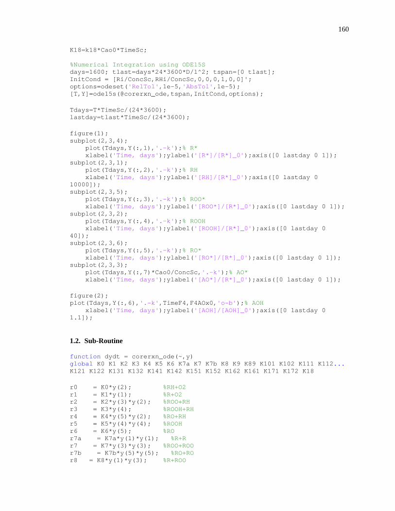
160

K18=k18*Cao0*TimeSc; %Numerical Integration using ODE15S days=1600; tlast=days*24*3600*D/l^2; tspan=[0 tlast ]; InitCond = [Ri/ConcSc,RHi/ConcSc,0,0,0,1,0,0]'; options=odeset( 'RelTol' ,1e-5, 'AbsTol' ,1e-5); [T,Y]=ode15s(@corerxn_ode,tspan,InitCond,options); Tdays=T*TimeSc/(24*3600); lastday=tlast*TimeSc/(24*3600); figure(1); subplot(2,3,4); plot(Tdays,Y(:,1), '.-k' ); % R* xlabel( 'Time, days' );ylabel( '[R*]/[R*]_0' );axis([0 lastday 0 1]); subplot(2,3,1); plot(Tdays,Y(:,2), '.-k' ); % RH xlabel( 'Time, days' );ylabel( '[RH]/[R*]_0' );axis([0 lastday 0 10000]); subplot(2,3,5); plot(Tdays,Y(:,3), '.-k' ); % ROO* xlabel( 'Time, days' );ylabel( '[ROO*]/[R*]_0' );axis([0 lastday 0 1]); subplot(2,3,2); plot(Tdays,Y(:,4), '.-k' ); % ROOH xlabel( 'Time, days' );ylabel( '[ROOH]/[R*]_0' );axis([0 lastday 0 40]); subplot(2,3,6); plot(Tdays,Y(:,5), '.-k' ); % RO* xlabel( 'Time, days' );ylabel( '[RO*]/[R*]_0' );axis([0 lastday 0 1]); subplot(2,3,3); plot(Tdays,Y(:,7)*Cao0/ConcSc, '.-k' ); % AO* xlabel( 'Time, days' );ylabel( '[AO*]/[R*]_0' );axis([0 lastday 0 1]);

figure(2); plot(Tdays,Y(:,6), '.-k' ,TimeF4,F4AOx0, 'o-b' ); % AOH xlabel( 'Time, days' );ylabel( '[AOH]/[AOH]_0' );axis([0 lastday 0 1.1]);

1.2. Sub-Routine

function dydt = corerxn_ode(~,y) global K0 K1 K2 K3 K4 K5 K6 K7a K7 K7b K8 K9 K89 K101 K10 2 K111 K112 ... K121 K122 K131 K132 K141 K142 K151 K152 K162 K161 K171 K 172 K18 r0 = K0*y(2); %RH+O2 r1 = K1*y(1); %R+O2 r2 = K2*y(3)*y(2); %ROO+RH r3 = K3*y(4); %ROOH+RH r4 = K4*y(5)*y(2); %RO+RH r5 = K5*y(4)*y(4); %ROOH r6 = K6*y(5); %RO r7a = K7a*y(1)*y(1); %R+R r7 = K7*y(3)*y(3); %ROO+ROO r7b = K7b*y(5)*y(5); %RO+RO r8 = K8*y(1)*y(3); %R+ROO

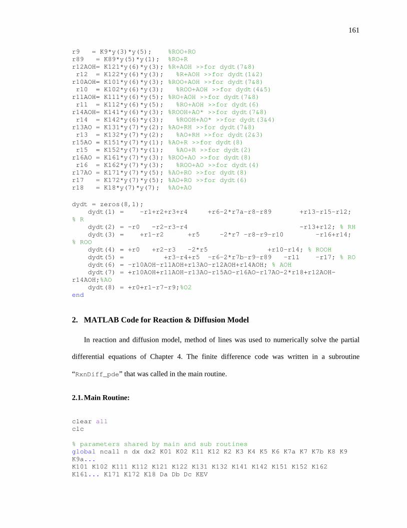
161

r9 = K9*y(3)*y(5); %ROO+RO r89 = K89*y(5)*y(1); %RO+R r12AOH= K121*y(6)*y(3); %R+AOH >>for dydt(7&8) r12 = K122*y(6)*y(3); %R+AOH >>for dydt(1&2) r10AOH= K101*y(6)*y(3); %ROO+AOH >>for dydt(7&8) r10 = K102*y(6)*y(3); %ROO+AOH >>for dydt(4&5) r11AOH= K111*y(6)*y(5); %RO+AOH >>for dydt(7&8) r11 = K112*y(6)*y(5); %RO+AOH >>for dydt(6) r14AOH= K141*y(6)*y(3); %ROOH+AO* >>for dydt(7&8) r14 = K142*y(6)*y(3); %ROOH+AO* >>for dydt(3&4) r13AO = K131*y(7)*y(2); %AO+RH >>for dydt(7&8) r13 = K132*y(7)*y(2); %AO+RH >>for dydt(2&3) r15AO = K151*y(7)*y(1); %AO+R >>for dydt(8) r15 = K152*y(7)*y(1); %AO+R >>for dydt(2) r16AO = K161*y(7)*y(3); %ROO+AO >>for dydt(8) r16 = K162*y(7)*y(3); %ROO+AO >>for dydt(4) r17AO = K171*y(7)*y(5); %AO+RO >>for dydt(8) r17 = K172*y(7)*y(5); %AO+RO >>for dydt(6) r18 = K18*y(7)*y(7); %AO+AO dydt = zeros(8,1); dydt(1) = -r1+r2+r3+r4 +r6-2*r7a-r8-r89 +r13-r15-r12; % R dydt(2) = -r0 -r2-r3-r4 -r13+r12; % RH dydt(3) = +r1-r2 +r5 -2*r7 -r8-r9-r 10 -r16+r14; % ROO dydt(4) = +r0 +r2-r3 -2*r5 +r 10-r14; % ROOH dydt(5) = +r3-r4+r5 -r6-2*r7b-r9-r89 -r11 -r17; % RO dydt(6) = -r10AOH-r11AOH+r13AO-r12AOH+r14AOH; % AOH dydt(7) = +r10AOH+r11AOH-r13AO-r15AO-r16AO-r17A O-2*r18+r12AOH-r14AOH; %AO dydt(8) = +r0+r1-r7-r9; %O2 end

2. MATLAB Code for Reaction & Diffusion Model

In reaction and diffusion model, method of lines was used to numerically solve the partial

differential equations of Chapter 4. The finite difference code was written in a subroutine

“RxnDiff_pde ” that was called in the main routine.

2.1. Main Routine:

clear all clc % parameters shared by main and sub routines global ncall n dx dx2 K01 K02 K11 K12 K2 K3 K4 K5 K6 K7a K7 K7b K8 K9 K9a... K101 K102 K111 K112 K121 K122 K131 K132 K141 K142 K 151 K152 K162 K161... K171 K172 K18 Da Db Dc KEV

162

% Values of Base Case Parameters l=0.16; % actual distance of samples from core to surface k0=10^-8; % rate constant for RH+O2 -> ROOH k1=10^9; % rate constant for free radical oxidation R*+O2 -> ROO* k2=1; % rate constant for ROO*+RH -> ROOH+R* (10^3>k2>10^ -4) k3RH=10^-5; % product of RH and rate constant for catalytic ROO H % degradation % ROOH+RH -> RO*+R*+H2O, this parameter control the "initial slope" k5=0; % rate constant for catalytic ROOH degradation by t ransition metal ions % 2ROOH -> RO*+ROO*+H2O k4=10; % rate constant for RO*+RH -> ROH+R* k6=1; % rate constant for RO* -> R=O+R* (this causes C-C breakage) k7=10^4; % rate constant for bimolecular ROO* terminations k8=0; % rate constant for ROO* terminating with R* (insig nificant) k9=0; % rate constant for ROO* terminating with RO* (insi gnificant) k7a=0; k7b=0; k9a=0; % Rate constants for other (insignificant) bimolecular % radical termination k10=10^7; % rate constant for ROO* stabilized by AO k11=10^7; % rate constant for RO* stabilized by AO k12=0; % rate constant for R* stabilized by AO (insignific ant) k13=0.025; % rate constant for AO*+RH -> AOH+R* k14=100; % rate constant for AO*+ROOH -> AOH+ROO* k16=9*10^8; % rate constant for termination of ROO* with AO* (t his parameter % controls the "asymptotic [AOH]") k15=10^9; % rate constant for termination of R* with AO* k17=10^9; % rate constant for termination of RO* with AO* ra dicals k18=10^3; % rate constant for AO* terminating with AO* RHi=10^-4; % initial RH concentration Ri=10^-8; % initial R* concentration Daoh=10^-10; % Diffusion coefficient for AOH Dao=10^-10; % Diffusion coefficient for AO* Do2=10^-7; % Diffusion coefficient for O2 D=10^-8; % Scaling factor for Diffusion coefficients Cao0_F1=8.75*10^-6; % Initial [AOH] for NeatPE1010 Cao0_F2=8.37*10^-6; % Initial [AOH] for Comp1010 Cao0_F3=4.53*10^-6; % Initial [AOH] for NeatPE1076 Cao0_F4=4.15*10^-6; % Initial [AOH] for Comp1076 Cao0=Cao0_F2; % Assigning which initial [AOH] to be used Co2s=10^-6; % Saturated [O2] at surface layer kev=100; % rate of AOH surface evaporation (exaggerated) Caos=2*10^-10; % Ratio of solubility of AOH in sample to air % Non-Dimentional form Da=Do2/D; Db=Daoh/D; Dc=Dao/D; KEV=kev*Caos*l/Dao; ConcSc = Ri; % concentration scaling factor TimeSc = l^2/D; % time scaling factor K01=k0*ConcSc*TimeSc; K02=k0*Co2s*TimeSc; K11=k1*ConcSc*TimeSc; K12=k1*Co2s*TimeSc; K2=k2*ConcSc*TimeSc;

163

K3=k3RH*TimeSc; K4=k4*ConcSc*TimeSc; K5=k5*ConcSc*TimeSc; K6=k6*TimeSc; K7a=k7a*ConcSc*TimeSc; K7=k7*ConcSc*TimeSc; K7b=k7b*ConcSc*TimeSc; K8=k8*ConcSc*TimeSc; K9=k9*ConcSc*TimeSc; K9a=k9a*ConcSc*TimeSc; K101=k10*ConcSc*TimeSc; K102=k10*Cao0*TimeSc; K111=k11*ConcSc*TimeSc; K112=k11*Cao0*TimeSc; K121=k12*ConcSc*TimeSc; K122=k12*Cao0*TimeSc; K131=k13*ConcSc*TimeSc; K132=k13*Cao0*TimeSc; K141=k14*ConcSc*TimeSc; K142=k14*Cao0*TimeSc; K151=k15*ConcSc*TimeSc; K152=k15*Cao0*TimeSc; K161=k16*ConcSc*TimeSc; K162=k16*Cao0*TimeSc; K171=k17*ConcSc*TimeSc; K172=k17*Cao0*TimeSc; K18=k18*Cao0*TimeSc; % Spacial Grid n=101;dx=1.0/(n-1);x=0.0:dx:1.0; dx2=1/dx^2; % Setting initial Conditions O20=zeros(1,n);R0=zeros(1,n);RH0=zeros(1,n);ROO0=ze ros(1,n); ROOH0=zeros(1,n);RO0=zeros(1,n);AOH0=zeros(1,n);AO0 =zeros(1,n); y0=zeros(1,8*n); for i=1:n if (i==n), O20(i)=1.0; else O20(i)=0.0; end R0(i)=Ri/ConcSc; RH0(i)=RHi/ConcSc; ROO0(i)=0.0; ROOH0(i)=0.0; RO0(i)=0.0; AOH0(i)=1.0; AO0(i)=0.0; y0(i)=O20(i);y0(i+n)=R0(i);y0(i+2*n)=RH0(i) ;y0(i+3*n)=ROO0(i); y0(i+4*n)=ROOH0(i);y0(i+5*n)=RO0(i);y0(i+6*n)=AOH0( i); y0(i+7*n)=AO0(i); end % Time to plot tabs=[0, 30*24*3600, 60*24*3600, 90*24*3600, 120*24 *3600, 150*24*3600, ... 180*24*3600, 210*24*3600, 240*24*3600, 270*24*3 600, 300*24*3600, ... 330*24*3600, 360*24*3600, 390*24*3600, 420*24*3 600, 450*24*3600];

164

tout=tabs*D/l^2;nout=numel(tabs); ncall=0; % ODE Integration reltol=1.0e-06; abstol=1.0e-06; options=odeset( 'RelTol' ,reltol, 'AbsTol' ,abstol); [t,y]=ode15s(@RxnDiff_pde,tout,y0,options); % 1 vector to 8 vectors O2=zeros(1,n); R=zeros(1,n);RH=zeros(1,n);ROO=zeros(1,n);ROOH=zero s(1,n); RO=zeros(1,n); AOH=zeros(1,n); AO=zeros(1,n); t otAOH=zeros(1,nout); totO2=zeros(1,nout); for it=1:nout for i=1:n O2(it,i)=y(it,i);R(it,i)=y(it,i+n); RH(it,i)=y(it,i+2*n);ROO(it,i)=y(it ,i+3*n); ROOH(it,i)=y(it,i+4*n);RO(it,i)=y(i t,i+5*n); AOH(it,i)=y(it,i+6*n);AO(it,i)=y(it ,i+7*n); end totAOH(it)=dx*trapz(AOH(it,:)); totO2(it)=dx*trapz(O2(it,:)); end figure(1); subplot(1,2,1);plot (x,O2);xlabel( 'x' );ylabel( '[O_2](x,t)' );axis tight ; subplot(1,2,2);plot (x,AOH);xlabel( 'x' );ylabel( '[AOH] / [AOH]_0' );axis([0 1 0 1]); figure(2); subplot(2,3,4);plot (x,R);xlabel( 'x' );ylabel( '[R*]/[R*]_0' );axis tight ; subplot(2,3,1);plot (x,RH);xlabel( 'x' );ylabel( '[RH]/[R*]_0' );axis tight ; subplot(2,3,5);plot (x,ROO);xlabel( 'x' );ylabel( '[ROO*]/[R*]_0' );axis tight ; subplot(2,3,2);plot (x,ROOH);xlabel( 'x' );ylabel( '[ROOH]/[R*]_0' );axis tight ; subplot(2,3,6);plot (x,RO);xlabel( 'x' );ylabel( '[RO*]/[R*]_0)' );axis tight ; subplot(2,3,3);plot (x,AO);xlabel( 'x' );ylabel( '[AO*]/[AOH]_0' );axis tight ;

2.2. Sub-Routine

function yt=RxnDiff_pde(t,y) global ncall n dx dx2 K01 K02 K11 K12 K2 K3 K4 K5 K6 K7a K7 K7b K8 K9 K9a... K101 K102 K111 K112 K121 K122 K131 K132 K141 K1 42 K151 K152 K162 ... K161 K171 K172 K18 Da Db Dc KEV % 1 vector to 8 vector O2=zeros(1,n);R=zeros(1,n);RH=zeros(1,n);ROO=zeros( 1,n); ROOH=zeros(1,n);RO=zeros(1,n);AOH=zeros(1,n);AO=zer os(1,n);

165

for i=1:n O2(i)=y(i); R(i)=y(i+n); RH(i)=y(i+2*n); ROO(i)=y(i+3*n); ROOH(i)=y(i+4*n); RO(i)=y(i+5*n); AOH(i)=y(i+6*n); AO(i)=y(i+7*n); end % PDEs and BCs (FD) for i=2:n %Surface Boundary condition, when i=n if (i==n), O2t(i)=0; Rt(i)=Rt(i-1); RHt(i)=RHt(i-1); ROOt(i)=ROOt(i-1); ROOHt(i)=ROOHt(i-1); ROt(i)=ROt(i-1); AOHt(i)=Db*(AOH(i-1)-AOH(i)*(1+KEV*dx))*dx2 -K101*AOH(i)*ROO(i) ... -K111*AOH(i)*RO(i)-K121*AOH(i)*R(i)+K131*AO(i)*RH(i)+K141*AO(i)*ROOH(i ); AOt(i)=AOt(i-1); else O2t(i)=Da*(O2(i+1)-2*O2(i)+O2(i-1))*dx2-K11*O2(i)* R(i)-K01*O2(i)*RH(i); Rt(i)=-K12*O2(i)*R(i)+K2*ROO(i)*RH(i)+K3*R OOH(i) ... +K4*RO(i)*RH(i)+K6*RO(i)-2*K7a*R(i)*R( i)-K8*R(i)*ROO(i) ... -K9a*RO(i)*R(i)-K122*R(i)*AOH(i)+K132* AO(i)*RH(i)-K152*AO(i)*R(i); RHt(i)=-K02*RH(i)*O2(i)-K2*ROO(i)*RH(i)-K3 *ROOH(i) ... -K4*RO(i)*RH(i)+K122*R(i)*AOH(i)-K132* AO(i)*RH(i); ROOt(i)=K12*O2(i)*R(i)-K2*ROO(i)*RH(i)+K5* ROOH(i)*ROOH(i) ... -2*K7*ROO(i)*ROO(i)-K8*R(i)*ROO(i)-K9* ROO(i)*RO(i) ... -K102*AOH(i)*ROO(i)+K142*AO(i)*ROOH(i) -K162*ROO(i)*AO(i); ROOHt(i)=K02*RH(i)*O2(i)+K2*ROO(i)*RH(i)-K 3*ROOH(i) ... -2*+K5*ROOH(i)*ROOH(i)+K102*AOH(i)*ROO (i)-K142*AO(i)*ROOH(i); ROt(i)=K3*ROOH(i)-K4*RO(i)*RH(i)+K5*ROOH(i )*ROOH(i) ... -K102*RO(i)*AO(i)-K6*RO(i)-2*K7b*RO(i) *RO(i)-K9*ROO(i)*RO(i) ... -K9a*RO(i)*R(i)-K112*RO(i)*AOH(i)-K172 *AO(i)*RO(i); AOHt(i)=Db*(AOH(i+1)-2*AOH(i)+AOH(i-1))*dx 2-K101*AOH(i)*ROO(i) ... -K111*AOH(i)*RO(i)-K121*AOH(i)*R(i)+K131*AO(i)*RH(i)+K141*AO(i)*ROOH(i ); AOt(i)=Dc*(AO(i+1)-2*AO(i)+AO(i-1))*dx2+K1 01*AOH(i)*ROO(i) ... +K111*AOH(i)*RO(i)+K121*AOH(i)*R(i)-K1 31*AO(i)*RH(i) ... -K141*AO(i)*ROOH(i)-K151*AO(i)*R(i)-K1 61*AO(i)*ROO(i) ... -K171*AO(i)*RO(i)-2*K18*AO(i)*AO(i); end end

166

% Symmetery Boundary condition at center, when i=1 O2t(1)=O2t(2); Rt(1)=Rt(2); RHt(1)=RHt(2); ROOt(1)=ROOt(2); ROOHt(1)=ROOHt(2); ROt(1)=ROt(2); AOHt(1)=AOHt(2); AOt(1)=AOt(2); % 8 vector to 1 vector for i=1:n yt(i)=O2t(i);yt(i+n)=Rt(i);yt(i+2*n)=RHt(i);yt( i+3*n)=ROOt(i); yt(i+4*n)=ROOHt(i);yt(i+5*n)=ROt(i);yt(i+6*n)=AOHt( i);yt(i+7*n)=AOt(i); end yt=yt'; ncall=ncall+1;

167

Appendix B: Estimation of ²° from the work of Korcek et al.[60]

As per our understanding, the rate constants (� ) of various H-abstraction by � · according

to Korcek et al.[60] can be estimated from the correlations developed by them. The correlations

for secondary and tertary � · are shown below by equations 30 and 31 respectively.

oÎ×]� ^ g 16.4 J 0.2 � ��� J �� B1

oÎ×]� ^ g 15.4 J 0.2 � ��� J �� B2

where, � is in units of ‘per active H’/(mol-s), and ��� J �� is the dissociation energy in

kcal/mol.

The values of ��� J �� for various molecules (that are small compared to polymeric

molecules) are given in Table 4 of the paper some of which are tabulated in Table S4 below:

Table S4. Carbon – hydrogen bond dissociation energies of various hydrocarbons

i · Æ�i J &�, kcal/mol

Primary

"��"� 98

"��"� "� 98

Secondary

]"��^ "� 95

"��"� ]"��^"� 95

Tertiary

]"��^�"Ø 92

Allyl

"� g "�"� 88

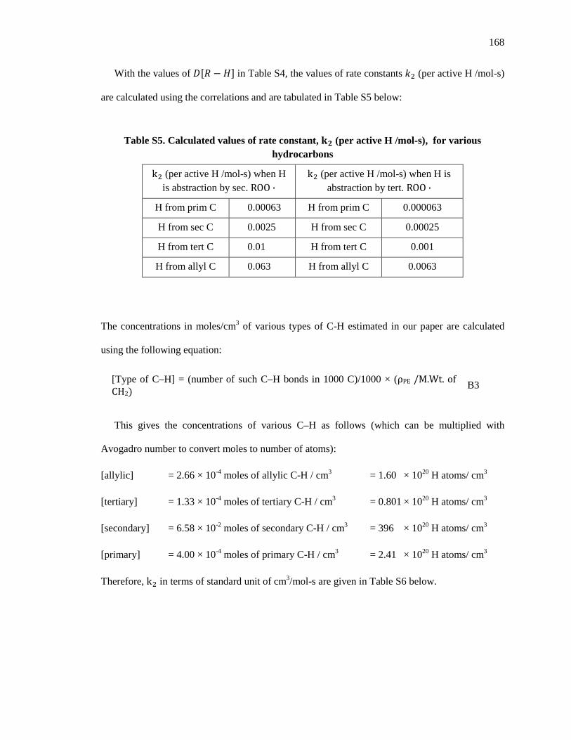
168

With the values of ��� J �� in Table S4, the values of rate constants � (per active H /mol-s)

are calculated using the correlations and are tabulated in Table S5 below:

Table S5. Calculated values of rate constant, k° (per active H /mol-s), for various hydrocarbons

k (per active H /mol-s) when H is abstraction by sec. ROO ·

k (per active H /mol-s) when H is abstraction by tert. ROO ·

H from prim C 0.00063 H from prim C 0.000063

H from sec C 0.0025 H from sec C 0.00025

H from tert C 0.01 H from tert C 0.001

H from allyl C 0.063 H from allyl C 0.0063

The concentrations in moles/cm3 of various types of C-H estimated in our paper are calculated

using the following equation:

[Type of C–H] = (number of such C–H bonds in 1000 C)/1000 × (ρPE /M.Wt. of CH2^ B3

This gives the concentrations of various C–H as follows (which can be multiplied with

Avogadro number to convert moles to number of atoms):

[allylic] = 2.66 × 10-4 moles of allylic C-H / cm3 = 1.60 × 1020 H atoms/ cm3

[tertiary] = 1.33 × 10-4 moles of tertiary C-H / cm3 = 0.801 × 1020 H atoms/ cm3

[secondary] = 6.58 × 10-2 moles of secondary C-H / cm3 = 396 × 1020 H atoms/ cm3

[primary] = 4.00 × 10-4 moles of primary C-H / cm3 = 2.41 × 1020 H atoms/ cm3

Therefore, k in terms of standard unit of cm3/mol-s are given in Table S6 below.

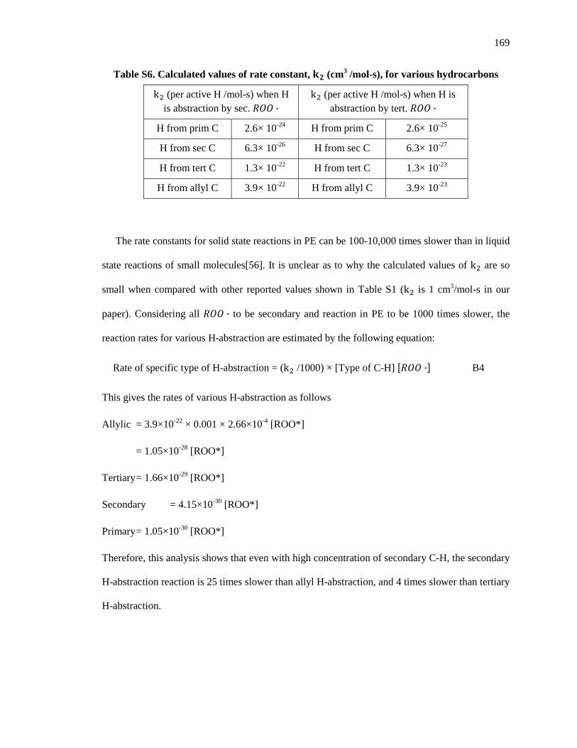
169

Table S6. Calculated values of rate constant, k° (cm3 /mol-s), for various hydrocarbons

k (per active H /mol-s) when H is abstraction by sec. � ·

k (per active H /mol-s) when H is abstraction by tert. � ·

H from prim C 2.6× 10-24 H from prim C 2.6× 10-25

H from sec C 6.3× 10-26 H from sec C 6.3× 10-27

H from tert C 1.3× 10-22 H from tert C 1.3× 10-23

H from allyl C 3.9× 10-22 H from allyl C 3.9× 10-23

The rate constants for solid state reactions in PE can be 100-10,000 times slower than in liquid

state reactions of small molecules[56]. It is unclear as to why the calculated values of k are so

small when compared with other reported values shown in Table S1 (k is 1 cm3/mol-s in our

paper). Considering all � · to be secondary and reaction in PE to be 1000 times slower, the

reaction rates for various H-abstraction are estimated by the following equation:

Rate of specific type of H-abstraction = (k /1000) × [Type of C-H] �� ·� B4

This gives the rates of various H-abstraction as follows

Allylic = 3.9×10-22 × 0.001 × 2.66×10-4 [ROO*]

= 1.05×10-28 [ROO*]

Tertiary = 1.66×10-29 [ROO*]

Secondary = 4.15×10-30 [ROO*]

Primary = 1.05×10-30 [ROO*]

Therefore, this analysis shows that even with high concentration of secondary C-H, the secondary

H-abstraction reaction is 25 times slower than allyl H-abstraction, and 4 times slower than tertiary

H-abstraction.

170

Vita

Iftekhar Ahmad

Place of Birth: Malda, India

Date of Birth: March 9, 1982

Country of citizenship: India

Education

• PhD, Chemical Engineering, December 2014 Drexel University, Philadelphia, PA

• Master of Technology, Polymer Technology, May 2007 Institute of Chemical Technology, Mumbai, India

• Bachelor of Technology, Petrochemical Engineering, May 2004 Aligarh Muslim University, Aligarh, India

Experience

• Assistant Manager, Wilmar Bioenrgi Indonesia, Feb-08 to Feb-09 • Academic Experience

o Graduate Research Assistant, Drexel University, Philadelphia, Jan-11 onwards

o Graduate Teaching Assistant, Drexel University, Philadelphia, Sep-09 to

Publications

• I. Ahmad, G. Hsuan, C.Y. Li, and R.A. Cairncross, ‘Reaction Model Describing Antioxidant Depletion in Polyethylene-Clay Nanocomposites Under Thermal Aging’, Polymer Degradation & Stability, 2014, Vol. 110, pages 318-335.

• W. K. Wong, S. Cheng, C. Y. Li, I. Ahmad, R. A. Cairncross, and Y. G. Hsuan, ‘Depletion Mechanism of Antioxidants in MDPE-Clay Nanocomposites under Thermal Aging’, Polymer Degradation & Stability, 2012, Vol. 97, Issue 2, pages 192-199.

• I. Ahmad, S. Cheng, C. Wong, G. Hsuan, C.Y. Li, and R.A. Cairncross, ‘A Reaction-Diffusion Model Describing Antioxidant Depletion in PE-Clay Nanocomposites Under Thermal Aging,’, Proceedings of ANTEC@NPE2012, Orlando, FL, April 2-4, 2012.

• S. Cheng, W. K. Wong, I. Ahmad, Y. G. Hsuan, C. Y. Li, and R. Cairncross, ‘Use Oxidative Induction Time to Evaluate Antioxidants in Polyethylene Clay Nanocomposite,’ Proceedings of North American Thermal Analysis Society-38th Annual Conference, Philadelphia (2010).

• I. Ahmad and P. A. Mahanwar, ‘Mechanical Properties of Fly Ash filled High Density Polyethylene’ The Journal of Minerals and Materials Characterization and Engineering, 2010, Vol. 9, No. 3, pages 183-198.